hep-th/0408072

A note on the non-commutative
dynamics of spinning D0 branes

Duane Loh , Kit Rodolfa and  Vatche Sahakian

Keck Laboratory

Harvey Mudd

Claremont, CA 91711, USA

Rotational dynamics is known to polarize D0 branes into higher dimensional fuzzy D$p$-branes: the tension forces between D0 branes provide the centripetal acceleration, and a puffed up spinning configuration stabilizes. In this work, we consider a rotating cylindrical formation of finite height, wrapping a compact cycle of the background space along the axis of rotation. We find an intriguing relation between the angular speed, the geometry of the cylinder, and the scale of non-commutativity; and we point out a critical radius corresponding to the case where the area of the cylinder is proportional to the number of D0 branes - reminiscent of Matrix black holes.

1 Introduction and results

D0 branes are natural probes of Planckian dynamics [11]. In a particularly interesting regime, D0 brane coordinates are represented by non-commuting matrices; and one’s intuition stemming from a notion of smooth spacetime quickly falters. Non-commutative dynamics entails rich new physics, exotic conclusions, and is a testing ground for quantum gravity[3]-[7]. It is then useful to study toy systems involving configurations of D0 branes.

A particularly interesting phenomenon of D0 brane dynamics involves a higher dimensional D$p$-brane being dynamically weaved out of polarized D0 branes. Typically, background Ramond-Ramond (RR) fluxes are used to polarize the D0 brane network [27, 29]. More recently, Harmark and Savvidy [13] have demonstrated that spinning a spherical lump of D0 branes can also lead to a puffed up fuzzy system. In a dual picture, one would talk about a rotating ellipsoidal D2 brane with magnetic flux on the worldvolume. The basic stabilization mechanism involves balancing the tension of strings stretching between the D0 branes with the centripetal acceleration. In [33], it was shown that such a system is indeed classically stable. These configurations can be interesting settings for black brane computations. Similar structures had inspired the modeling of Matrix black holes whose thermodynamic properties had been shown to agree with that of black holes in Matrix theory [3, 15, 2, 4]. Yet another interest in D0 brane fuzz-balls arises in brane-world discussions. The worldvolume theory of the resulting higher dimensional D$p$-brane is inherently non-commutative and provides for interesting new phenomena at high energies, when the scale of non-commutativity is probed [34].

In this work, we consider a cylindrical configuration of D0 branes stabilized by spin. The cylinder is wrapped along its axis of rotation onto a compact cycle of the background space. Finite height cylinders are interesting since they allow one to explore the mixing of several length scales in a non-commutative setting: the size of the background compact cycle or the height of the cylinder, the radius of the cylinder, and the scale of non-commutativity. The size of the compact cycle may also be imagined to be infinite so as to generate an infinite cylinder, as in [1]. We would then have a non-commutative worldvolume theory with one non-compact and one compact direction; and the compact direction is stabilized dynamically through rotation.

Our problem is described by the following parameters (see Figure 1): $N$ is the number of D0

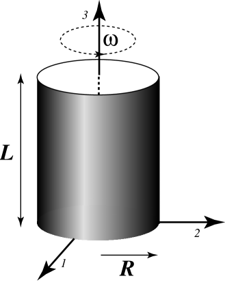
Figure 1: The coordinates system used to describe the fuzzy cylinder. The direction labeled $3$ is compact of size $L$.

branes; $L$ is the size of the compact cycle; $R$ is the radius of the cylinder; $\omega$ is the angular frequency of rotation; $w$ and $k_{1}$ are respectively the winding number along the compact cycle and the lateral winding number; finally, the string length $l_{s}$ sets the scale for lengths, and the string coupling $g_{s}$ is assumed to be small. To simplify matters, we fix $g_{s}$, $N$, $w$, and $k_{1}$ to convenient values, and think of the problem in terms of varying $L$, $R$, and $\omega$. The limit $L\rightarrow\infty$, $N\rightarrow\infty$ presumably corresponds to the infinite cylinder, which has been studied in the literature in various settings [1, 14, 29, 30].

To study the dynamics, we use the Dirac-Born-Infeld (DBI) action of [28, 27]. We summarize the highlights of our results whereas the details are left to the main text:

• We find that the angular speed $\omega$ is related to the other parameters by

  $$\omega=-\frac{4\pi wk_{1}L}{\lambda N}\ .$$ (1)

  The scale of non-commutativity on the worldvolume of the cylinder is $4\pi/N$ in string units. Our analysis is valid if

  $$\Omega\equiv\omega R\ll 1\ \ \ ,\ \ \ \omega l_{s}\ll 1$$ (2)

  which still leaves $R$ a free parameter. Hence, we now have a two parameter problem.

• In previous works [1, 14], the case of the infinite cylinder was studied and identified as BPS stable, with the radial extent $R$ being a flat direction free to be chosen at no cost in energy. In our work, we adopt a different representation of the algebra that can accommodate a wrapped cylinder of finite height; with $N$, the number of D0 branes, being finite as well. This involves the mixing of infinite and finite dimensional representations in a delicate recipe.

• We argue for the existence of a critical radius $R_{cr}$ given by

  $$R_{cr}=\frac{1}{\omega}\ ,$$ (3)

  corresponding to the case where the D0 branes are moving with the speed of light. If one considers the possibility that the conjectured symmetrized trace prescription of [28, 27] is valid to all orders in the DBI expansion for the simple matrix algebra we have, the action vanishes at this critical radius. This is reminiscent of giant graviton dynamics arising in a different context [6, 18, 22]. Furthermore, at $R_{cr}$, we have

  $$\mbox{Cylinder area}=\frac{\lambda N}{2}\ .$$ (4)

  With entropy $S\sim N$ for Matrix black holes [3, 15, 4] - which are qualitatively similar configurations - this is very suggestive of a holographic statement arising in a non-commutative theory at weak string coupling.

These conclusions lend themselves to interesting future directions that we discuss in the last section, where we also comment on the issue of classical radiation from the configuration. In Section 2, we setup the problem and present the solution to the equations of motion. In Section 3, we discuss the critical radius and the dynamics of perturbation modes. And some details of the perturbation analysis may be found in Appendix A.

Note Added: In the original version of the preprint, a numerical perturbation analysis was also presented, leading to the identification of unstable modes for certain ratios of the cylinder height to its radius. As pointed out in [1], the algebra describing the cylinder in question saturates a BPS bound, where the central charge is the cylinder’s angular momentum, the latter being proportional to the Casimir of the algebra. Hence, the expectation is that the cylinder must be stable in all regions of the parameter space and for all representations of the algebra. In the current version of the preprint, the numerical part of the perturbation analysis has been removed as it apparently leads to unreliable conclusions.

2 The fuzzy rotating cylinder

We start from the DBI action of [28, 27]

$$S_{DBI}=-T_{p}\int d^{p+1}\sigma\,\mbox{STr}\left[e^{-\phi}\sqrt{-\mbox{det}\left[\mbox{P}\left[E_{ab}+E_{ai}(Q^{-1}-\delta)^{ij}E_{jb}\right]+\lambda F_{ab}\right]}\sqrt{\mbox{det}Q^{i}_{j}}\right]\ ,$$ (5)

where

$$Q^{i}_{j}\equiv\delta^{i}_{j}+i\lambda\left[\Phi^{i},\Phi^{j}\right]\ \ \ \ ,\ \ \ \lambda\equiv 2\pi l_{s}^{2}\ ,$$ (6)

while the nine $\Phi^{i}$’s are $N\times N$ hermitian matrices representing the non-commutative coordinates of $N$ D$p$-branes. The tension of a D$p$ brane is given by

$$T_{p}=\frac{2\pi}{g_{s}\left(2\pi l_{s}\right)^{p+1}}\ ,$$ (7)

$\mbox{P}[]$ denotes the pullback to the D-brane worldvolume, and STr stands for the symmetrized trace [28, 27]. For the task at hand, we consider $N$ D0 branes and zero background fields. In particular, we have in (5)

$$E_{\mu\nu}\equiv G_{\mu\nu}+B_{\mu\nu}\rightarrow\eta_{\mu\nu}\ \ \ ,\ \ \ \phi\rightarrow 0\ ,$$ (8)

and the Chern-Simons term is vanishing. This leads to the action

$$S_{DBI}=-T_{0}\int dt\ \mbox{STr}\sqrt{1-\lambda^{2}{{\dot{\Phi^{i}}}}^{2}}\sqrt{\mbox{det}\left[\delta^{i}_{j}+i\lambda\left[\Phi^{i},\Phi^{j}\right]\right]}$$ (9)

where we have dropped a term of the form

$$\dot{\Phi}^{i}\dot{\Phi}^{j}\left[\Phi_{i},\Phi_{j}\right]\rightarrow 0$$ (10)

because of the symmetrized trace prescription, and we have chosen the non-dynamical gauge field on the worldline to be zero at the expense of imposing the constraint

$$\left[\dot{\Phi}^{i},\Phi_{i}\right]=0\ .$$ (11)

If we were interested in an approximate form of the dynamics, we can focus on the regime where

$$\dot{\Phi}^{i}\ll\frac{1}{l_{s}^{2}}\ \ \ \ ,\ \ \ \left[\Phi^{i},\Phi^{j}\right]\ll\frac{1}{l_{s}^{2}}\ \ \ ,\ \ \ \ddot{\Phi}^{i}\ll\frac{1}{l_{s}^{3}}\ .$$ (12)

We then arrive at the simpler expression

$$S_{DBI}\simeq=-T_{0}\int dt\ \mbox{STr}\left[1-\frac{\lambda^{2}}{2}\left({D_{0}{\Phi^{i}}}\right)^{2}-\frac{\lambda^{2}}{4}\left[\Phi^{i},\Phi^{j}\right]^{2}+\cdots\right]\ ,$$ (13)

where the covariant derivative has been reintroduced

$$D_{0}\Phi^{i}=\dot{\Phi}^{i}+i\left[A_{0},\Phi^{i}\right]$$ (14)

for future reference. For now, we set $A_{0}=0$ as mentioned above. The equations of motion are

$$\ddot{\Phi}^{i}=\left[\Phi^{j},\left[\Phi^{i},\Phi_{j}\right]\right]\ .$$ (15)

supplemented by the constraint (11).

2.1 A time-dependent solution

Next, our goal is to find a solution to the equations of motion (15) subject to the constraint (11) representing $N$ D0 branes forming a fuzzy cylinder of finite height and rotating about its axis of symmetry. We start by singling out three of the space dimensions for embedding the cylinder. We label these three directions by $\Phi^{i}$, with $i=1,2,3$. Furthermore, we compactify the direction $i=3$ on a circle of circumference $L$ on which we intend to wrap the longitudinal extent of the cylinder (see Figure 1). The remaining six transverse polarizations will be denoted by $\Phi^{a}$.

Consider a hermitian matrix $\hat{Y}$, and another matrix $\hat{Z}$ with its complex conjugate $\hat{Z}^{\dagger}$, satisfying the closed algebra

$$\left[\hat{Z},\hat{Z}^{\dagger}\right]=0\ \ \ ,\ \ \ \left[\hat{Z},\hat{Y}\right]=\omega\hat{Z}\ \ \ ,\ \ \ \left[\hat{Z}^{\dagger},\hat{Y}\right]=-\omega\hat{Z}^{\dagger}\ ,$$ (16)

where $\omega$ is a real constant. We will talk about the representation of this algebra in the next section. We construct two new matrices from $\Phi^{1}$ and $\Phi^{2}$

$$Z\equiv\Phi^{1}+i\Phi^{2}\ \ \ ,\ \ \ Z^{\dagger}=\Phi^{1}-i\Phi^{2}\ .$$ (17)

And we write

$$Z=z(t)\hat{Z}\ \ \ ,\ \ \ \Phi^{3}=\frac{wL}{\lambda}\hat{Y}\ \ \ \ ,\ \ \ \Phi^{a}=0\ .$$ (18)

We have arranged for the cylinder to wind the $3$ direction $w$ times, with $w$ being an arbitrary integer. It is then easy to check that this ansatz satisfies the constraint (11) and the equations (15) provided we have

$$z(t)=\frac{R}{\lambda}e^{i\omega t}\ .$$ (19)

Here, $R$ is the radius of the rotating cylinder as shown in Figure 1.

2.2 Algebra representation

To proceed with analyzing the properties and perturbations of the solution we found in the previous section, we need to identify a representation of the algebra (16). The representation we adopt is worked out in detail in [37], custom designed to depict a wrapped fuzzy cylinder. We first introduce two new operators $\rho$ and $\sigma$

$$\hat{Y}=\rho\ \ \ ,\ \ \ \hat{Z}=e^{ik_{1}\sigma}\ ,$$ (20)

satisfying the infinite dimensional algebra.

$$\left[\sigma,\rho\right]=\frac{4\pi i}{N}\ .$$ (21)

$k_{1}$ is an integer that appears to represent the number of lateral windings of the cylinder. Given the compactification in the $\rho$ direction, we may partially truncate this representation as described in [37]. We focus on $N$ being an odd integer with $N=2M+1$. A basis of $N\times N$ matrices that describes a wrapped non-commutative cylinder is

$$e(k^{\prime})\equiv e^{{k^{\prime}}_{1}\sigma+i{k^{\prime}}_{2}\rho}\ .$$ (22)

where ${k^{\prime}}=({k^{\prime}}_{1},{k^{\prime}}_{2})$ represents a pair of integers

$${k^{\prime}}_{1}=p^{\prime}N+q^{\prime}\ \ \ \ \mbox{with}\ \ \ q^{\prime}\in\left(-M,M\right)\ \ \ \mbox{and}\ \ \ p^{\prime}\in\left(-\infty,\infty\right)\ ;$$ (23)

$${k^{\prime}}_{2}=m^{\prime}\ \ \ \ \mbox{with}\ \ \ m^{\prime}\in\left(-M,M\right)\ .$$ (24)

Note in particular that the modes for ${k^{\prime}}_{2}$ have been truncated. The algebra satisfied by these basis matrices is

$$\left[e(k^{\prime}),e(k^{\prime\prime})\right]=-2i\sin\left(\frac{2\pi}{N}k^{\prime}\times k^{\prime\prime}\right)e(k^{\prime}+k^{\prime\prime})\ ,$$ (25)

where $k^{\prime}\times k^{\prime\prime}={k^{\prime}}_{1}{k^{\prime\prime}}_{2}-{k^{\prime}}_{2}{k^{\prime\prime}}_{1}$. And

$$\left[\rho,e(k^{\prime})\right]=\frac{4\pi{k^{\prime}}_{1}}{N}e(k^{\prime})\ .$$ (26)

The explicit forms are given by [37]

$$\rho\rightarrow-2\pi i\partial_{\theta}\left(\begin{array}[]{ccccc}1&&&&\\ &1&&&\\ &&1&&\\ &&&\ddots&\\ &&&&1\end{array}\right)+4\pi\left(\begin{array}[]{ccccc}\frac{M}{N}&&&&\\ &\frac{M-1}{N}&&&\\ &&\frac{M-2}{N}&&\\ &&&\ddots&\\ &&&&-\frac{M}{N}\end{array}\right)\ .$$ (37)

$$e^{i(p^{\prime}N+q^{\prime})\sigma+im^{\prime}\rho}\rightarrow$$

$$\left\{\begin{array}[]{cl}\tau^{p^{\prime}}\gamma^{-m^{\prime}(q^{\prime}+1)}\left(\begin{array}[]{cccccc}\overbrace{0\ \ \cdots\ \ 0}^{q^{\prime}}&1&&&&\\ &0&\gamma^{-2m^{\prime}}&&&\\ &&\ddots&\ddots&&\\ &&&&0&\gamma^{-2(N-q^{\prime}-1)m^{\prime}}\\ \gamma^{-2(N-q^{\prime})m^{\prime}}\tau&&&&&0\\ \ddots&&&&&\vdots\\ \underbrace{0\ \ \cdots\ \ 0}_{q^{\prime}-1}&\gamma^{-2(N-1)m^{\prime}}\tau&&&&0\end{array}\right)&q^{\prime}>0\\ \tau^{p^{\prime}}\gamma^{-m^{\prime}}\left(\begin{array}[]{ccccc}1&&&&\\ &\gamma^{-2m^{\prime}}&&&\\ &&\gamma^{-4m^{\prime}}&&\\ &&&\ddots&\\ &&&&\gamma^{-2(N-1)m^{\prime}}\end{array}\right)\ \ \ \ \ \ \ \ \ \ \ q^{\prime}=0&\\ \tau^{p^{\prime}-1}\gamma^{-m^{\prime}(q^{\prime}+1)}\left(\begin{array}[]{cccccc}\overbrace{0\ \ \cdots\ \ 0}^{N+q^{\prime}}&1&&&&\\ &0&\gamma^{-2m^{\prime}}&&&\\ &&\ddots&\ddots&&\\ &&&&0&\gamma^{-2(-q^{\prime}-1)m^{\prime}}\\ \gamma^{-2(-q^{\prime})m^{\prime}}\tau&&&&&0\\ \ddots&&&&&\vdots\\ \underbrace{0\ \ \cdots\ \ 0}_{N+q^{\prime}-1}&\gamma^{-2(N-1)m^{\prime}}\tau&&&&0\end{array}\right)&q^{\prime}<0\end{array}\right.$$ (60)

Here, we have defined

$$\tau=e^{2\,i\theta}\ \ \ ,\ \ \ \gamma=e^{\frac{2\pi i}{N}}\ ,$$ (61)

where $\theta$ is a parameter used to label the infinite dimensional sector of the representation.

Tracing in this representation becomes

$$\mbox{Tr}\rightarrow\int d\theta\ \mbox{Tr}\ .$$ (62)

We then have the orthogonality statement

$$\mbox{Tr}\left[e(k^{\prime})e(k^{\prime\prime})\right]=e^{-\frac{2\pi i}{N}k^{\prime}\times k^{\prime\prime}}\mbox{Tr}\left[e(k^{\prime}+k^{\prime\prime})\right]=N\delta_{k^{\prime},-k^{\prime\prime}}\ ;$$ (63)

and we also get

$$\hat{Z}\hat{Z^{\dagger}}=\mbox{1}\ \ \ \,\ \ \ {\hat{Z}}^{N}=\tau^{k_{1}}\ .$$ (64)

With these expressions at hand, we may now verify that

$${\Phi^{1}}^{2}+{\Phi^{2}}^{2}=\frac{R^{2}}{\lambda^{2}}\mbox{{\bf 1}}\ .$$ (65)

It is also easy to check that our solution carries angular momentum in the 3 direction given by

$$M_{12}\equiv T_{0}\lambda^{2}\mbox{Tr}\left[\dot{\Phi}^{2}\Phi^{1}-\dot{\Phi}^{1}\Phi^{2}\right]=T_{0}NR^{2}\omega\ ;$$ (66)

while the other components are zero. $\omega$ is obviously the angular speed about the $3$ axis. More interestingly, we find from (26) that we need

$$\omega=-\frac{4\pi wLk_{1}}{\lambda N}\ .$$ (67)

Note that $w$ is the number of windings of the cylinder in the $3$ directions, $k_{1}$ is the number of windings in the lateral direction, and $4\pi/N$ is the scale of non-commutativity on the cylinder’s worldvolume in string units. Hence, the angular speed is fixed once the representation is fixed. We may make the intuitive statement that the angular speed in units of $R$ is the ratio of the area of the cylinder to the number of D0 branes $N$.

3 A critical radius and perturbations of the cylinder

Our solution is parameterized by the following constants: $N$, the number of D0 branes; $R$, the radius of the cylinder; $L$, the compact size of the $3$ direction; $\omega$, the angular speed; and two integers $w$ and $k_{1}$ representing windings. $\omega$ however was fixed in the previous section (see equation (67)). For fixed $N$, $w$ and $k_{1}$, we are then dealing with a two parameter problem, $R$ and $L$.

The solution is valid provided the conditions (12) are satisfied. This translates to

$$\Omega=\omega R\ll 1\ \ \ \ ,\ \ \ \omega l_{s}\ll 1\ .$$ (68)

Hence, $R$ is unrestricted. We also note that $\omega\ll 1/l_{s}$ may be independently achieved by making either $L$ small or $N$ large.

First, we observe that one can now write

$$\mbox{det}\left[\delta^{i}_{j}+i\lambda\left[\Phi^{i},\Phi^{j}\right]\right]=1+\lambda^{2}\omega^{2}|z|^{2}\ .$$ (69)

Substituting our solution in (9), the full form of the action, we get

$$S_{DBI}=-T_{0}N\int dt\ \sqrt{1-\Omega^{4}}\ .$$ (70)

However, this assumes that the symmetrized trace prescription is good for arbitrary order in the expansion of the square roots in (9). While it is possible that, for this particular simple algebra, additional corrections to the DBI - as well as corrections to the symmetrized trace prescription - may vanish, this assumption is generally incorrect. For now, our goal however is to use the guess to the extent of corroborating the existence of a critical maximum radius for which the D0 branes are moving with the speed of light. And indeed as confirmed from equation (70), this radius is

$$R_{cr}=\frac{1}{\omega}\ ,$$ (71)

for which the potential (and action) vanishes. Furthermore, we then have

$$\left(2\pi R_{cr}\right)L=\frac{\lambda N}{2}\ .$$ (72)

Hence, the area of the cylinder equals $\lambda N/2$, an interesting holographic statement as eluded to in the Introduction.

Next, we consider the dynamics of perturbations of the cylinder for $\Omega\ll 1$. We would then write

$$\Phi^{1}=\Phi^{1}_{0}+{\hat{\phi}}^{1}\ \ \ \ ,\ \ \ \Phi^{2}=\Phi^{2}_{0}+{\hat{\phi}}^{2}\ \ \ \ ,\ \ \ \Phi^{3}=\Phi^{3}_{0}+{\hat{\phi}}^{3}\ \ \ \ ,\ \ \ \Phi^{a}={\hat{\phi}}^{a}\ \ \ \ ,\ \ \ A_{0}=\hat{a}\ ,$$ (73)

where the $0$ subscripts refer to the solution of the previous sections. Note that we fluctuate the gauge field $A_{0}$ of (14) as well. We will then use the equation of motion arising from varying $a$ to restrict perturbation modes to physical degrees of freedom. It is more convenient to parameterize some of these perturbations differently. We write instead

$${\hat{\phi}}^{1}=-(\Phi^{2}_{0}\hat{\epsilon}_{\theta}+\hat{\epsilon}_{\theta}\Phi^{2}_{0})+(\Phi^{1}_{0}\hat{\epsilon}_{r}+\hat{\epsilon}_{r}\Phi^{1}_{0})\ .$$ (75)

$${\hat{\phi}}^{2}=(\Phi^{1}_{0}\hat{\epsilon}_{\theta}+\hat{\epsilon}_{\theta}\Phi^{1}_{0})+(\Phi^{2}_{0}\hat{\epsilon}_{r}+\hat{\epsilon}_{r}\Phi^{2}_{0})\ .$$ (76)

Now, we expand the small perturbations in the matrix basis of the previous section

$$\hat{\epsilon}_{\theta}=\sum_{k^{\prime}}\theta_{k^{\prime}}e(k^{\prime})\ \ \ \ ,\ \ \ \ \hat{\epsilon}_{r}=\sum_{k^{\prime}}r_{k^{\prime}}e(k^{\prime})\ .$$ (77)

$${\hat{\phi}}^{3}=\sum_{k^{\prime}}\frac{\epsilon^{3}_{k^{\prime}}}{R}e(k^{\prime})\ \ \ \ ,\ \ \ \ {\hat{\phi}}^{a}=\sum_{k^{\prime}}\frac{\epsilon^{a}_{k^{\prime}}}{R}e(k^{\prime})\ \ \ \ ,\ \ \ \ \hat{a}=\sum_{k^{\prime}}{a_{k^{\prime}}}e(k^{\prime})\ .$$ (78)

Note that we have made sure that $\epsilon^{3}_{k^{\prime}}$ and $\epsilon^{a}_{k^{\prime}}$ are dimensionless for convenience; and we have reality conditions relating modes of opposite signs, such as $r_{k^{\prime}}^{*}=r_{-k^{\prime}}$. We also use the shorthand (see equations (23) and (24))

$$\sum_{k^{\prime}}\equiv\sum_{p^{\prime}=-\infty}^{\infty}\sum_{q^{\prime}=-M}^{M}\sum_{m^{\prime}=-M}^{M}\ ,$$ (79)

To assure that an expansion in the $\varepsilon$’s makes sense, we require

$$r_{k^{\prime}},\theta_{k^{\prime}}\ll 1\ \ \ ,\ \ \ {{\varepsilon}}^{3}_{k^{\prime}}\ll\frac{N\omega R}{4\pi k_{1}}\ .$$ (80)

Substituting (73) into (13), and using the commutation relations

$$\left[\Phi^{3}_{0},e(k^{\prime})\right]=\frac{wL}{\lambda}\frac{4\pi{k^{\prime}}_{1}}{N}e(k^{\prime})\ ;$$ (81)

$$\left[Z_{0},e(k^{\prime})\right]=-2i\frac{R}{\lambda}e^{i\omega t}\sin\left(\frac{2\pi}{N}k\times k^{\prime}\right)e(k+k^{\prime})\ ;$$ (82)

$$\left[Z^{\dagger}_{0},e(k^{\prime})\right]=2i\frac{R}{\lambda}e^{-i\omega t}\sin\left(\frac{2\pi}{N}k\times k^{\prime}\right)e(-k+k^{\prime})\ ,$$ (83)

one can write the worldvolume theory of small perturbations. We emphasize that this analysis is restricted to the regime prescribed by (68).

As far as perturbation modes in the six transverse directions are concerned, we find that all these modes are diagonal with mass squared given by

$$m_{trans}^{2}={\frac{4R^{2}}{\lambda^{2}}{\sin^{2}\left(\frac{2\,\pi\,{k_{1}}\,{l_{2}}}{N}\right)}+{\omega}^{2}\,\frac{{{l_{1}}}^{2}}{k_{1}^{2}}}>0\ ,$$ (84)

where $l_{1}$ and $l_{2}$ are integers to be described below.

The interesting physics occurs in the 1-2-3 subspace where there are two physical degrees of freedom (due to the constraint in the system). The details of this analysis are collected in Appendix A. The final action is given by $S_{1}+S_{2}+S_{3}$, where $S_{1}$, $S_{2}$, and $S_{3}$ are defined in (87), (88), and (90) respectively.

4 Discussion

We end with a few comments about the matter of classical radiation. In the dual picture, the system is to be described by a cylindrical D2 brane with magnetic and electric fields on the worldvolume accounting for the dissolved D0 branes and rotation. It is easy to see that, from this static viewpoint, one expects zero radiation from the RR 1-form gauge field. In the picture involving the D0 branes explicitly, zero 1-form radiation is a much more non-trivial statement. Yet, it is expected that the conclusion agrees with the dual picture, presumably the two being related by some Seiberg-Witten map [34]. Considering the Chern-Simons coupling from [27], one easily finds

$$C_{i}=\frac{J_{i}(k,\omega)}{{\vec{k}}^{2}-\omega^{2}}\ ,$$ (85)

where $C_{i}(k,\omega)$ is the Fourier mode of the 1-form RR gauge field. The source is identified as [27]

$$J_{i}(k,\omega)\simeq\int dt\ e^{-i\omega t}\mbox{STr}\left[e^{-i\lambda\Phi^{j}k_{j}}{\dot{\Phi}}^{i}\right]\ .$$ (86)

Considering linear order in $\lambda$, it is easy to check that $\mbox{STr}[\Phi^{j}{\dot{\Phi}}^{i}]$ is time independent resulting in zero radiated power. Indeed, one can see that this pattern repeats to all orders: we have $\dot{Z}=\omega Z$ and ${\dot{Z}}^{\dagger}=-\omega Z^{\dagger}$; and hence terms of the form $\mbox{STr }x\cdots x$ where $x$ stands for a $Z$ or a $Z^{\dagger}$ (wavefronts cannot have a component in the 3 direction by symmetry). The number of $Z$’s and $Z^{\dagger}$’s must equal so that the trace does not vanish (see in particular equation (64)). But this also cancels all time dependences from the source leaving zero radiated power through the RR 1-form. This suggests that the symmetrized trace prescription and the DBI action seem to be working well for our solution to all orders in $\lambda$. It would also be interesting to see what conclusions are reached with regards to gravitational and RR 3-form radiation.

5 Appendix A: Some details of the perturbation analysis

In this appendix, we collect some of the details of the perturbation analysis. For notational convenience, we relabel some of the perturbations as $\theta_{k^{\prime}}\equiv\epsilon_{k^{\prime}}^{1}$ and $r_{k^{\prime}}\equiv\epsilon_{k^{\prime}}^{2}$. Expanding our action to quadratic order (for $\epsilon_{k^{\prime}}^{1},\epsilon_{k^{\prime}}^{2}\ll 1$, ${{\epsilon}}^{3}_{k^{\prime}}\ll{N\omega R}/{4\pi k_{1}}$) in the small perturbations, one finds three pieces after a bit of algebra: from the kinetic term without the gauge field fluctuations taken into account, we get

$$S_{1} = N\,R^{2}\,{\omega}^{2}+4\,N\,R^{2}\,{\omega}^{2}\,{\epsilon}_{0}^{2}+4\,N\,R^{2}\,\omega\,{{\dot{\epsilon}}_{0}}^{1}$$ (87)

$$+ 4\,N\,R^{2}\,{\cos^{2}(\frac{2\,\pi\,k\times l}{N})}\,\left({{\dot{\epsilon}}^{1}_{-l}}+\omega\,{\epsilon}_{-l}^{2}\right)\,\left({{\dot{\epsilon}}^{1}_{l}}+\omega\,{\epsilon}_{l}^{2}\right)$$

$$+ 4\,N\,R^{2}\,{\cos^{2}\left(\frac{2\,\pi\,k\times l}{N}\right)}\,\left({{\dot{\epsilon}}^{2}_{-l}}-\omega\,{\epsilon}_{-l}^{1}\right)\,\left({{\dot{\epsilon}}^{2}_{l}}-\omega\,{\epsilon}_{l}^{1}\right)$$

$$+ N\,{\lambda}^{2}\,{{\dot{\epsilon}}^{3}_{-l}}\,{{\dot{\epsilon}}^{3}_{l}}+N\,{\lambda}^{2}\,{{{\dot{\epsilon}}^{a}}_{-l}}\,{{\dot{\epsilon}}^{a}_{l}}\ .$$

From the quartic potential, we obtain

$$S_{2} = -N\,R^{2}\,{\omega}^{2}-4\,N\,R^{2}\,{\omega}^{2}\,{\epsilon}_{0}^{2}-{4\,N\,R^{2}\,{\omega}^{2}\,{\cos^{2}\left(\frac{2\,\pi\,k\times l}{N}\right)}\,{\left(1+\frac{{{l_{1}}}^{2}}{{{k_{1}}}^{2}}\right)}\,{\epsilon}_{-l}^{1}\,{\epsilon}_{l}^{1}}$$ (88)

$$- {8\,i\,N\,R^{2}\,{\omega}^{2}\,{\cos^{2}\left(\frac{2\,\pi\,k\times l}{N}\right)}\,\frac{l_{1}}{k_{1}}\,{\epsilon}_{-l}^{2}\,{\epsilon}_{l}^{1}}+{8\,i\,N\,R^{2}\,{\omega}^{2}\,{\cos^{2}\left(\frac{2\,\pi\,k\times l}{N}\right)}\,\frac{l_{1}}{k_{1}}\,{\epsilon}_{-l}^{1}\,{\epsilon}_{l}^{2}}$$

$$+ {4\,N\,R^{2}\,{\cos^{2}\left(\frac{2\,\pi\,k\times l}{N}\right)}\,\left(-2\,\frac{R^{2}}{\lambda^{2}}-{\omega}^{2}+2\,\frac{R^{2}}{\lambda^{2}}\,\cos\left(\frac{4\,\pi\,k\times l}{N}\right)\,-\,{\omega}^{2}\,\frac{{{l_{1}}}^{2}}{k_{1}^{2}}\right)\,{\epsilon}_{-l}^{2}\,{\epsilon}_{l}^{2}}$$

$$- {2\,N\,R^{2}\,\omega\,\sin(\frac{4\,\pi\,k\times l}{N})\,\frac{{{l}}_{1}}{k_{1}}\,{\epsilon}_{-l}^{3}\,{\epsilon}_{l}^{1}}-{2\,N\,R^{2}\,\omega\,\sin\left(\frac{4\,\pi\,k\times l}{N}\right)\,\frac{{{l}}_{1}}{k_{1}}\,{\epsilon}_{-l}^{1}\,{\epsilon}_{l}^{3}}$$

$$+ 4\,i\,N\,R^{2}\,\omega\,\sin\left(\frac{4\,\pi\,k\times l}{N}\right)\,{\epsilon}_{-l}^{3}\,{\epsilon}_{l}^{2}-4\,i\,N\,R^{2}\,\omega\,\sin\left(\frac{4\,\pi\,k\times l}{N}\right)\,{\epsilon}_{-l}^{2}\,{\epsilon}_{l}^{3}$$

$$- 4\,N\,R^{2}\,{\sin^{2}\left(\frac{2\,\pi\,k\times l}{N}\right)}\,{\epsilon}_{-l}^{3}\,{\epsilon}_{l}^{3}-{N\,\left(4\,R^{2}\,{\sin^{2}\left(\frac{2\,\pi\,k\times l}{N}\right)}+{\lambda}^{2}\,{\omega}^{2}\,\frac{{{l_{1}}}^{2}}{k_{1}^{2}}\right)\,{\epsilon}_{-l}^{a}\,{\epsilon}_{l}^{a}}\ .$$

Finally, we solve the equations of motion for the gauge field fluctuation modes $a_{l}$

$$a_{l} = -\frac{2\,i\,{k_{1}^{2}}\,R^{2}}{4\,R^{2}\,{\sin^{2}\left(\frac{2\,\pi\,k\times l}{N}\right)}\,{{k_{1}}}^{2}+{\lambda}^{2}\,{\omega}^{2}\,{{l_{1}}}^{2}}$$ (89)

$$\times \left(2\,\omega\,{\cos^{2}\left(\frac{2\,\pi\,k\times l}{N}\right)}\,{\epsilon}_{l}^{1}-\sin\left(\frac{4\,\pi\,k\times l}{N}\right)\,\left({{\dot{\epsilon}}_{l}}^{1}+2\,\,\omega\,{\epsilon}_{l}^{2}\right)+{\lambda}^{2}\,\frac{\omega}{2\,R^{2}}\,\frac{l_{1}}{k_{1}}\,{{\dot{\epsilon}}^{3}_{l}}\right)$$

and substitute back into the action; this gives the additional piece

$$S_{3} = -\frac{N\,R^{4}}{4\,R^{2}\,{\sin^{2}\left(\frac{2\,\pi\,k\times l}{N}\right)}\,{{k_{1}}}^{2}+{\lambda}^{2}\,{\omega}^{2}\,{{l_{1}}}^{2}}$$ (90)

$$\times \,\left(\frac{{\lambda}^{2}}{R^{2}}\,\omega\,{l_{1}}\,{{\dot{\epsilon}}^{3}_{-l}}+4\,\omega\,{\cos^{2}\left(\frac{2\,\pi\,k\times l}{N}\right)}\,{k_{1}}\,{\epsilon}_{-l}^{1}-2\,{{{k}}_{1}}\,\sin\left(\frac{4\,\pi\,k\times l}{N}\right)\,\left({{\dot{\epsilon}}_{-l}^{1}}+2\,\omega\,{\epsilon}_{-l}^{2}\right)\right)$$

$$\times \left(\frac{{\lambda}^{2}}{R^{2}}\,\omega\,{l_{1}}\,{{\dot{\epsilon}}^{3}_{l}}+4\,\omega\,{\cos^{2}\left(\frac{2\,\pi\,k\times l}{N}\right)}\,{k_{1}}\,{\epsilon}_{l}^{1}-2\,{{{k}}_{1}}\,\sin\left(\frac{4\,\pi\,k\times l}{N}\right)\,\left({{\dot{\epsilon}}_{l}^{1}}+2\,\omega\,{\epsilon}_{l}^{2}\right)\right)$$

Our system is now given by $S_{1}+S_{2}+S_{3}$.

References

- [1] Dongsu Bak and Ki-Myeong Lee. Noncommutative supersymmetric tubes. Phys. Lett., B509:168–174, 2001, hep-th/0103148.
- [2] Tom Banks, W. Fischler, and Igor R. Klebanov. Evaporation of schwarzschild black holes in matrix theory. Phys. Lett., B423:54–58, 1998, hep-th/9712236.
- [3] Tom Banks, W. Fischler, Igor R. Klebanov, and Leonard Susskind. Schwarzschild black holes from matrix theory. Phys. Rev. Lett., 80:226–229, 1998, hep-th/9709091.
- [4] Tom Banks, W. Fischler, Igor R. Klebanov, and Leonard Susskind. Schwarzschild black holes in matrix theory. II. JHEP, 01:008, 1998, hep-th/9711005.
- [5] Adel Bilal. Higher-derivative corrections to the non-abelian Born- Infeld action. Nucl. Phys., B618:21–49, 2001, hep-th/0106062.
- [6] John H. Brodie, Leonard Susskind, and N. Toumbas. How Bob Laughlin tamed the giant graviton from Taub-Nut space. JHEP, 02:003, 2001, hep-th/0010105.
- [7] Yi-Fei Chen and J. X. Lu. Dynamical brane creation and annihilation via a background flux. 2004, hep-th/0405265.
- [8] Jan de Boer, Eric Gimon, Koenraad Schalm, and Jeroen Wijnhout. Evidence for a gravitational Myers effect. 2002, hep-th/0212250.
- [9] Jan de Boer, Koenraad Schalm, and Jeroen Wijnhout. General covariance of the non-abelian DBI-action: Checks and balances. 2003, hep-th/0310150.
- [10] Robbert Dijkgraaf, Erik Verlinde, and Herman Verlinde. Matrix string theory. Nucl. Phys., B500:43–61, 1997, hep-th/9703030.
- [11] Michael R. Douglas, Daniel Kabat, Philippe Pouliot, and Stephen H. Shenker. D-branes and short distances in string theory. Nucl. Phys., B485:85–127, 1997, hep-th/9608024.
- [12] R. Gregory and R. Laflamme. Black strings and p-branes are unstable. Phys. Rev. Lett., 70:2837–2840, 1993, hep-th/9301052.
- [13] Troels Harmark and Konstantin G. Savvidy. Ramond-Ramond field radiation from rotating ellipsoidal membranes. Nucl. Phys., B585:567–588, 2000, hep-th/0002157.
- [14] Koji Hashimoto. The shape of non-abelian D-branes. JHEP, 04:004, 2004, hep-th/0401043.
- [15] Gary T. Horowitz and Emil J. Martinec. Comments on black holes in matrix theory. Phys. Rev., D57:4935–4941, 1998, hep-th/9710217.
- [16] Wung-Hong Huang. Condensation of tubular D2-branes in magnetic field background. 2004, hep-th/0405192.
- [17] Yoshifumi Hyakutake. Notes on the construction of the D2-brane from multiple D0- branes. Nucl. Phys., B675:241–269, 2003, hep-th/0302190.
- [18] Bert Janssen, Yolanda Lozano, and Diego Rodriguez-Gomez. A microscopical description of giant gravitons. ii: The AdS(5) x S(5) background. Nucl. Phys., B669:363–378, 2003, hep-th/0303183.
- [19] N. Ohta and J.-G. Zhou, Nucl. Phys. B522 (1998) 125, hep-th/9801023,
- [20] D. Bak and N. Ohta, Phys. Lett. B527 (2002) 131, hep-th/0112034,
- [21] Y. Hyakutake and N. Ohta, Phys. Lett. B539 (2002) 153, hep-th/0204161.
- [22] Bert Janssen, Yolanda Lozano, and Diego Rodriguez-Gomez. Giant gravitons in AdS(3) x S(3) x T**4 as fuzzy cylinders. 2004, hep-th/0406148.
- [23] Paul Koerber and Alexander Sevrin. The non-abelian born-infeld action through order alpha’**3. JHEP, 10:003, 2001, hep-th/0108169.
- [24] Miao Li, Emil J. Martinec, and Vatche Sahakian. Black holes and the SYM phase diagram. Phys. Rev., D59:044035, 1999, hep-th/9809061.
- [25] David Mateos and Paul K. Townsend. Supertubes. Phys. Rev. Lett., 87:011602, 2001, hep-th/0103030.
- [26] Lubos Motl. Proposals on nonperturbative superstring interactions. 1997, hep-th/9701025.
- [27] Robert C. Myers. Dielectric-branes. JHEP, 12:022, 1999, hep-th/9910053.
- [28] A. A. Tseytlin. On non-abelian generalisation of the Born-Infeld action in string theory. Nucl. Phys., B501:41–52, 1997, hep-th/9701125.
- [29] Subodh P. Patil. D0 matrix mechanics: New fuzzy solutions at large N. 2004, hep-th/0406219.
- [30] Subodh P Patil. D0 matrix mechanics: Topological dynamics of fuzzy spaces. 2004, hep-th/0407182.
- [31] S. Ramgoolam, B. Spence, and S. Thomas. Resolving brane collapse with 1/N corrections in non- abelian DBI. 2004, hep-th/0405256.
- [32] Vatche Sahakian. Transcribing spacetime data into matrices. JHEP, 06:037, 2001, hep-th/0010237.
- [33] Konstantin G. Savvidy and George K. Savvidy. Stability of the rotating ellipsoidal D0-brane system. Phys. Lett., B501:283–288, 2001, hep-th/0009029.
- [34] Nathan Seiberg and Edward Witten. String theory and noncommutative geometry. JHEP, 09:032, 1999, hep-th/9908142.
- [35] IV Taylor, Washington and Mark Van Raamsdonk. Multiple D0-branes in weakly curved backgrounds. Nucl. Phys., B558:63–95, 1999, hep-th/9904095.
- [36] IV Taylor, Washington and Mark Van Raamsdonk. Multiple Dp-branes in weak background fields. Nucl. Phys., B573:703–734, 2000, hep-th/9910052.
- [37] Shozo Uehara and Satoshi Yamada. Wrapped membranes, matrix string theory and an infinite dimensional Lie algebra. 2004, hep-th/0402012.
- [38] Vitor Cardoso and Jos’e Lemos. New instability for rotating black branes and strings. 2004, hep-th/0412078.
- [39] Giovanni Arcioni and Ernesto Lozano-Tellechea. Stability and Critical Phenomena of Black Holes and Black Rings. 2004, hep-th/0412118.