Noncommutative Conformally Coupled Scalar Field Cosmology and its Commutative Counterpart

Abstract

We study the implications of a noncommutative geometry of the minisuperspace variables for the FRW universe with a conformally coupled scalar field. The investigation is carried out by means of a comparative study of the universe evolution in four different scenarios: classical commutative, classical noncommutative, quantum commutative, and quantum noncommutative, the last two employing the Bohmian formalism of quantum trajectories. The role of noncommutativity is discussed by drawing a parallel between its realizations in two possible frameworks for physical interpretation: the NC-frame, where it is manifest in the universe degrees of freedom, and in the C-frame, where it is manifest through $\theta$-dependent terms in the Hamiltonian. As a result of our comparative analysis, we find that noncommutative geometry can remove singularities in the classical context for sufficiently large values of $\theta$. Moreover, under special conditions, the classical noncommutative model can admit bouncing solutions characteristic of the commutative quantum FRW universe. In the quantum context, we find non-singular universe solutions containing bounces or being periodic in the quantum commutative model. When noncommutativity effects are turned on in the quantum scenario, they can introduce significant modifications that change the singular behavior of the universe solutions or that render them dynamical whenever they are static in the commutative case. The effects of noncommutativity are completely specified only when one of the frames for its realization is adopted as the physical one. Non-singular solutions in the NC-frame can be mapped into singular ones in the C-frame.

I Introduction

Over the latest years a great deal of work and effort has been done in the direction of understanding canonical noncommutative field theories and quantum mechanics (see 1 ; 2 and references therein). The recent interest in these theories is motivated by works that establish a connection between noncommutative geometry and string theory 3 . Intensive research is carried out to investigate their interesting properties, such as the IR-UV mixing and nonlocality 5 , Lorentz violation 6 , new physics at very short distances 1 ; 2 , and the equivalence between translations in the noncommutative directions and gauge transformations (see, e.g. 2 ; 6.5 ).

Several investigations have been pursued to verify the possible role of noncommutativity in a great deal of cosmological scenarios. Among them we quote Newtonian cosmology 11 , cosmological perturbation theory and inflationary cosmology 12 , noncommutative gravity 14 , and quantum cosmology 15 ; 16 . In a previous work 16 , an investigation into the influence of noncommutativity of the minisuperspace variables in the early universe scenario was carried out for the Kantowski-Sachs universe. Although noncommutativity effects proved to be relevant to the universe history at intermediate times, they were shown not to be capable of removing the future and past cosmological singularities of that model in the classical context. In the quantum context, on the other hand, non-singular universe solutions were shown to be present. However, since they exist for the commutative quantum Kantowski-Sachs universe, their presence in the ensemble of solutions of the noncommutative quantum model cannot be attributed to the noncommutativity effects.

Although the investigation carried out in 16 was restricted to a particular model, one expected that some of the results obtained there could be of general validity. Indeed, in this work we shall show that noncommutativity can appreciably modify the evolution of the Friedman-Robertson-Walker (FRW) universe with a conformally coupled scalar field 17 ; 18 . As in reference 16 , our investigation is carried out by means of a comparative study of the universe evolution in four different scenarios: classical commutative, classical noncommutative, quantum commutative and quantum noncommutative. The main motivation for the choice of the conformally coupled scalar field is that it admits exact solutions in the simpler cases discussed along this work and it is rich enough to be useful as a probe for the significant modifications noncommutative geometry introduces in classical and quantum cosmologies. The analytical treatment renders easy the study of the singular behavior of the model in its four versions. As we shall show later, even in the classical context noncommutative geometry can remove singularities. Moreover, depending on the value of the noncommutative parameter, noncommutative classical models can mimic quantum effects.

As an interpretation for quantum theory, we are adopting the Bohmian one, which we briefly review in section 4. Originally proposed by Bohm in 1952 19 , and further developed by him in a collaboration with Hiley 19.2 , such an interpretation of quantum theory has acquired an increasing number of adepts along the years 19.3 . Decisive contributions for the development of the Bohmian quantum physics were made by Bell 19.4 , who was its arduous defender for three decades, by Holland 20 , and by D. Dürr, S. Goldstein and N. Zanghì (see, e.g., 20.3 -20.7 and ref. therein). Due to the capability it has to reproduce the experimental results of quantum mechanics and quantum field theory providing an intuitive interpretation of the underlying dynamics, Bohmian quantum physics is presently an issue of interest for broad community (see, e.g., 21 ). In this work the main reason that compels us to adopt the Bohmian interpretation in quantum cosmology is the absence of external observers in the primordial quantum universe, which renders the standard Copenhagen interpretation inapplicable in its description. As an alternative, the Bohmian interpretation has been employed in several works of quantum cosmology and quantum gravity (see, e.g., 16 ; 18 ; 22 ). Other interesting aspect of the Bohmian approach to quantum theory, which motivates us for its adoption, is the efficient framework it provides for comparison between the classical and quantum counterparts of a physical model in the common language of trajectories. We shall benefit from this facility in our comparative study of the four versions of the FRW universe. Since our preference for Bohmian interpretation is justified for technical, rather than philosophical reasons, we shall not focus our discussion on fundamental questions regarding the interpretation of quantum theory (for references on this subject see 18 ; 22.1 ). Instead, whenever possible, we shall give preference for the interpretation-independent aspects.

This work is organized as follows. Sections 2 and 3 are devoted to a comparative study of the classical FRW with a conformally coupled scalar field and its noncommutative counterpart. In section 4 we present the commutative quantum version of the model, and analyze it by using the Bohmian formalism of quantum trajectories. A similar study is carried out in sections 5 and 6, which are concerned with the noncommutative quantum version of the model. In section 7 we end up with a general discussion and summary of the main results.

II The Conformally Coupled Scalar Field Model

As a reference for the identification of the noncommutative effects later, it is interesting to consider first the commutative classical FRW universe, which we describe as follows. We shall restrict our considerations to the case of constant positive curvature of the spatial sections. The action for the conformally coupled scalar field model in this case is 18

$$S=\int d^{4}x\sqrt{-g}\left[-\frac{1}{2}\varphi_{;\mu}\varphi^{;\mu}+\frac{1}{16\pi G}R-\frac{1}{12}R\varphi^{2}\right],$$ (1)

where $g_{\mu\nu}$ is the four-metric, $g$ its determinant, $R$ is the scalar curvature, and $\varphi$ is the scalar field. Units are chosen such that $\hbar=c=1$ and $8\pi G=3l_{p}^{2}$, where $l_{p}$ is the Planck length. For the FRW model with an homogeneous scalar field the following ansatz of minisuperspace can be adopted

$$\left\{\begin{array}[c]{c}ds^{2}=-N^{2}(t)dt^{2}+a^{2}(t)\left[\frac{dr^{2}}{1-r^{2}}+r^{2}\left(d\theta^{2}+\sin^{2}\theta d\varphi^{2}\right)\right],\\ \\ \varphi=\varphi(t).\end{array}\right.$$ (2)

By substituting (2) in (1) and rescaling the scalar field as $\chi=\varphi al_{p}/\sqrt{2,}$ we have the following minisuperspace action

$$S=\int dt\left(Na-\frac{a\dot{a}^{2}}{N}+\frac{a\dot{\chi}^{2}}{N}-\frac{N\chi^{2}}{a}\right).$$ (3)

The corresponding Hamiltonian is

$$H=N\left[-\frac{P_{a}^{2}}{4a}+\frac{P_{\chi}^{2}}{4a}-a+\frac{\chi^{2}}{a}\right]=N\mathcal{H},$$ (4)

where the canonical momenta are

$$P_{a}=-\frac{2a\dot{a}}{N}\text{, \ \ }P_{\chi}=\frac{2a\dot{\chi}}{N}.$$ (5)

As the Poisson Brackets for the classical phase space variables we have

$$\left\{a,\chi\right\}=0,\text{ \ }\left\{a,P_{a}\right\}=1\text{, \ }\left\{\chi,P_{\chi}\right\}=1\text{,\ \ }\left\{P_{a},P_{\chi}\right\}=0.$$ (6)

The equations of motion for the metric and matter field variables $a$, $P_{a},$ $\chi$ and $P_{\chi}$ that follow from (4) and (6) are

$$\left\{\begin{array}[c]{c}\dot{a}=\left\{a,H\right\}=-NP_{a}/2a,\\ \\ \dot{P}_{a}=\left\{P_{a},H\right\}=2N,\\ \\ \dot{\chi}=\left\{\chi,H\right\}=NP_{\chi}/2a,\\ \\ \dot{P}_{\chi}=\left\{P_{\chi},H\right\}=-2N\chi/a.\end{array}\right.$$ (7)

From now on we shall adopt conformal time gauge $N=a.$ The general solution of (7) for $a$ and $\chi$ in this gauge is

$$a(t)=\left(A+C\right)\cos(t)+\left(B+D\right)\sin(t),$$ (8)

$$\chi(t)=\left(A-C\right)\cos(t)+\left(B-D\right)\sin(t),$$ (9)

where the super-Hamiltonian constraint $\mathcal{H}\approx 0$ imposes the relation

$$AC+BD=0.$$ (10)

As it can be seen, the classical commutative solutions are necessarily singular in the past and in the future. Figs. $1(a),(b),(c)$ and $(d)$ present plots of the solution for $a(t)$ in the dashed curves for given values of $A,B,$ and $C$ [$D$ is fixed by (10)].

III Noncommutative Deformation of the Classical Model

Let us introduce a noncommutative classical geometry in our universe model by keeping the Hamiltonian with the same functional form as (4), but now valued on noncommutative variables,

$$H=N\left[-\frac{P_{a_{nc}}^{2}}{4a_{nc}}+\frac{P_{\chi_{nc}}^{2}}{4a_{nc}}-a_{nc}+\frac{\chi_{nc}^{2}}{a_{nc}}\right],$$ (11)

where $a_{nc}$, $\chi_{nc}$, $P_{a_{nc}}$ and $P_{\chi_{nc}}$ satisfy the deformed Poisson brackets

$$\left\{a_{nc},\chi_{nc}\right\}=\theta,\text{ \ }\left\{a_{nc},P_{a_{nc}}\right\}=1\text{, \ }\left\{\chi_{nc},P_{\chi_{nc}}\right\}=1\text{,\ \ }\left\{P_{a_{nc}},P_{\chi_{nc}}\right\}=0.$$ (12)

By making the substitution

$$a_{nc}=a_{c}-\frac{\theta}{2}P_{\chi_{c}}\text{, \ }\chi_{nc}=\chi\text{${}_{c}+$}\frac{\theta}{2}P_{a_{c}}\text{,\ \ }P_{a_{c}}=P_{a_{nc}}\text{,\ \ }P_{\chi_{c}}=P_{\chi_{nc}},$$ (13)

the theory defined by (11) and (12) can be mapped into a theory where the metric and matter variables satisfy the Poisson brackets

$$\left\{a_{c},\chi_{c}\right\}=0,\text{ \ }\left\{a_{c},P_{a_{c}}\right\}=1\text{,\ \ }\left\{\chi_{c},P_{\chi_{c}}\right\}=1\text{,\ \ }\left\{P_{a_{c}},P_{\chi_{c}}\right\}=0.$$ (14)

Written in terms of $a_{c}$, $\chi_{c}$, $P_{a_{c}}$ and $P_{\chi_{c}},$ the Hamiltonian (11) exhibits the noncommutative content of the theory through $\theta$-dependent terms. Two distinct physical theories, one considering $a_{c}$ and $\chi_{c}$, and the other considering $a_{nc}$ and $\chi_{nc}$ as the physical scale factor and matter field can be assumed to emerge from (11), (12), (13) and (14). In the case where $a_{c}$ and $\chi_{c}$ are assumed as the preferred variables for physical interpretation, the theory can be interpreted as a “commutative” one with a modified interaction. We shall refer to this theory as being realized in the “C-frame”. To the other possible theory, which assumes $a_{nc}$ and $\chi_{nc}$ as the constituents of the physical metric and matter field, we shall refer as realized in the “NC-frame”. There are works that privilege the C-frame approach (e.g. 15 ), and others the NC-frame (e.g. 16 ; 22.2 ; 22.3 ). Some works rely on the assumption that the difference between C- and NC-variables is negligible (e.g. 22.7 ). However, as showed in 22.3 , even in simple models the difference in behavior between these two types of variables can be appreciable. In what follows we will show that in the cosmological scenario the assumption of the NC- or C-frame point of view as preferential for physical interpretation leads to dramatic differences in the analysis of the universe history. A parallel between the theories in both frames realizations is draw in the classical context here, and in the quantum context in section 6.

Methodologically, the route we shall follow in the computation of the configuration variables in this classical context is the same as that adopted in the noncommutative quantum case discussed later on. We shall depart from the C-frame and calculate $a_{c}(t)$, $\chi_{c}(t)$, $P_{a_{c}}(t),$ and $P_{\chi_{c}}(t)$. After that, we shall use (13) to obtain the corresponding $a_{nc}(t)$ and $\chi_{nc}(t)$ in the NC-frame. The computation of the physical quantities is rendered simpler by the gauge choice $N=a_{nc}$, which from now on will be assumed as the gauge employed in all calculations.

The equations of motion for the variables $a_{c}(t)$, $\chi_{c}(t)$, $P_{a_{c}}(t)$ and $P_{\chi_{c}}(t)$ are

$$\left\{\begin{array}[c]{c}\dot{a}_{c}=\left\{a_{c},H\right\}=-\frac{1}{2}\left(1-\theta^{2}\right)P_{a_{c}}+\theta\chi_{c},\\ \\ \dot{P}_{a_{c}}=\left\{P_{a_{c}},H\right\}=2a_{c}-\theta P_{\chi_{c}},\\ \\ \dot{\chi}_{c}=\left\{\chi_{c},H\right\}=\frac{1}{2}\left(1-\theta^{2}\right)P_{\chi_{c}}+\theta a_{c},\\ \\ \dot{P}_{\chi_{c}}=\left\{P_{\chi_{c}},H\right\}=-2\chi_{c}-\theta P_{a_{c}}.\end{array}\right.$$ (15)

According to the values of $\theta$, the system (15) allows three types of solutions, which we describe below.

III.0.1 Case $\left|\theta\right|<1$

The general solutions for $a_{c}(t)$, $\chi_{c}(t)$, $P_{a_{c}}(t)$ and $P_{\chi_{c}}(t)$ in the $\theta<1$ case are

$$\begin{array}[c]{c}a_{c}(t)=e^{\theta t}\left[A\sqrt{1-\theta^{2}}\cos\left(\sqrt{1-\theta^{2}}t\right)+B\sqrt{1-\theta^{2}}\sin\left(\sqrt{1-\theta^{2}}t\right)\right]\\ \\ +e^{-\theta t}\left[C\sqrt{1-\theta^{2}}\cos\left(\sqrt{1-\theta^{2}}t\right)+D\sqrt{1-\theta^{2}}\sin\left(\sqrt{1-\theta^{2}}t\right)\right],\end{array}$$ (16)

$$\begin{array}[c]{c}\chi_{c}(t)=e^{\theta t}\left[A\sqrt{1-\theta^{2}}\cos\left(\sqrt{1-\theta^{2}}t\right)+B\sqrt{1-\theta^{2}}\sin\left(\sqrt{1-\theta^{2}}t\right)\right]\\ \\ -e^{-\theta t}\left[C\sqrt{1-\theta^{2}}\cos\left(\sqrt{1-\theta^{2}}t\right)+D\sqrt{1-\theta^{2}}\sin\left(\sqrt{1-\theta^{2}}t\right)\right],\end{array}$$ (17)

$$P_{a_{c}}=2e^{\theta t}\left[-B\cos\left(\sqrt{1-\theta^{2}}t\right)+A\sin\left(\sqrt{1-\theta^{2}}t\right)\right]+2e^{-\theta t}\left[-D\cos\left(\sqrt{1-\theta^{2}}t\right)+C\sin\left(\sqrt{1-\theta^{2}}t\right)\right],$$ (18)

$$P_{\chi_{c}}=2e^{\theta t}\left[B\cos\left(\sqrt{1-\theta^{2}}t\right)-A\sin\left(\sqrt{1-\theta^{2}}t\right)\right]+2e^{-\theta t}\left[-D\cos\left(\sqrt{1-\theta^{2}}t\right)+C\sin\left(\sqrt{1-\theta^{2}}t\right)\right].$$ (19)

From (13), (16)-(19) we can calculate $a_{nc}(t)$ and $\chi_{nc}(t)$ as

$$\begin{array}[c]{c}a_{nc}(t)=e^{\theta t}\left\{\left[A\sqrt{1-\theta^{2}}-B\theta\right]\cos\left(\sqrt{1-\theta^{2}}t\right)+\left[B\sqrt{1-\theta^{2}}+A\theta\right]\sin\left(\sqrt{1-\theta^{2}}t\right)\right\}\\ \\ +e^{-\theta t}\left\{\left[C\sqrt{1-\theta^{2}}+D\theta\right]\cos\left(\sqrt{1-\theta^{2}}t\right)+\left[D\sqrt{1-\theta^{2}}-C\theta\right]\sin\left(\sqrt{1-\theta^{2}}t\right)\right\},\end{array}$$ (20)

$$\begin{array}[c]{c}\chi_{nc}(t)=e^{\theta t}\left\{\left[A\sqrt{1-\theta^{2}}-B\theta\right]\cos\left(\sqrt{1-\theta^{2}}t\right)+\left[B\sqrt{1-\theta^{2}}+A\theta\right]\sin\left(\sqrt{1-\theta^{2}}t\right)\right\}\\ \\ -e^{-\theta t}\left\{\left[C\sqrt{1-\theta^{2}}+D\theta\right]\cos\left(\sqrt{1-\theta^{2}}t\right)+\left[D\sqrt{1-\theta^{2}}-C\theta\right]\sin\left(\sqrt{1-\theta^{2}}t\right)\right\}.\end{array}$$ (21)

The constraint $\mathcal{H}\approx 0$ in the present case can be written as

$$\left(AC+BD\right)\sqrt{1-\theta^{2}}+\left(AD-BC\right)\theta=0.$$ (22)

In the limit where $\theta\rightarrow 0$, equation (22) is reduced to the equation (10). In the same limit, the NC- and C-frame solutions, given by (20)-(21) and (16)-(17), respectively, coincide and match with the commutative solutions (8) and (9).

From (16), (20) and (22) it can be seen that, as in the commutative case, $a_{nc}(t)$ and $a_{c}(t)$ are unavoidably singular in the past and in the future. The exponential multiplying factors in both solutions can model their shape giving rise to bounces at intermediate times, as is depicted in the thin and thick solid lines in Fig. $1(a)$ for representative values of $A,B$ and $C$ [$D$ is fixed by (22)].

Figure 1: The typical behavior of the scale factor of the noncommutative FRW universe in the NC-frame realization (thick lines) in contrast with C-frame realization (thin lines). The scale factor of the commutative counterpart appears plotted in the dashed lines. $(a)$: $\theta=3/4,$ $A=5,$ $B=3$ and $C=6$. $\left(b\right):\theta=1,$ $A=3,$ $B=2$ and $C=1$. $\left(c\right):\theta=3/2,$ $A=4,$ $B=3$ and $C=1$. $\left(d\right):\theta=3/2,$ $A=-1.2,$ $B=2$ and $C=-1$.

III.0.2 Case $\theta=\pm 1$

When $\theta=\pm 1,$ the solutions for $a_{c}(t)$, $\chi_{c}(t)$, $P_{a_{c}}(t)$ and $P_{\chi_{c}}(t)$ are

$$a_{c}(t)=A\cosh t+B\sinh t,$$ (23)

$$\chi_{c}(t)=\pm B\cosh t\pm A\sinh t,$$ (24)

$$P_{a_{c}}=2\left(D+At\right)\cosh t+2\left(C+Bt\right)\sinh t,$$ (25)

$$P_{\chi_{c}}=\mp 2\left(C+Bt\right)\cosh t\mp 2\left(D+At\right)\sinh t.$$ (26)

As the corresponding $a_{nc}(t)$ and $\chi_{nc}(t),$ we have

$$a_{nc}(t)=\left(A+C+Bt\right)\cosh t+\left(B+D+At\right)\sinh t,$$ (27)

$$\chi_{nc}(t)=\pm\left(B+D+At\right)\cosh t\pm\left(A+C+Bt\right)\sinh t.$$ (28)

The constraint $\mathcal{H}\approx 0$ in the present case can be written as

$$A^{2}-B^{2}+2\left(AC-BD\right)=0.$$ (29)

As it can be seen, the universe solutions in the case $\theta=\pm 1$ are characterized by a qualitative behavior that differs from the one corresponding to the case$\ \left|\theta\right|<1$. There exist non-singular bouncing solutions for both $a_{nc}(t)$ and $a_{c}(t)$, as depicted in Fig. $1(b)$. However, the correspondence between the NC- and C-frames can be broken for some values of the integration constants. Non-singular solutions in the NC-frame can correspond to singular solutions in the C-frame. An interesting example is the case where $A=B=0$ and $C>\left|D\right|$. This corresponds to a bouncing universe in the NC-frame that has no counterpart in the C-frame, where the universe is singular at all times.

III.0.3 Case $\left|\theta\right|>1$

The general solutions for $a_{c}(t)$, $\chi_{c}(t)$, $P_{a_{c}}(t)$ and $P_{\chi_{c}}(t)$ when $\left|\theta\right|>1\$are

$$\begin{array}[c]{c}a_{c}(t)=e^{\theta t}\left[A\sqrt{\theta^{2}-1}\cosh\left(\sqrt{\theta^{2}-1}t\right)+B\sqrt{\theta^{2}-1}\sinh\left(\sqrt{\theta^{2}-1}t\right)\right]\\ \\ +e^{-\theta t}\left[C\sqrt{\theta^{2}-1}\cosh\left(\sqrt{1-\theta^{2}}t\right)+D\sqrt{\theta^{2}-1}\sinh\left(\sqrt{\theta^{2}-1}t\right)\right],\end{array}$$ (30)

$$\begin{array}[c]{c}\chi_{c}(t)=e^{\theta t}\left[A\sqrt{\theta^{2}-1}\cosh\left(\sqrt{\theta^{2}-1}t\right)+B\sqrt{\theta^{2}-1}\sinh\left(\sqrt{\theta^{2}-1}t\right)\right]\\ \\ -e^{-\theta t}\left[C\sqrt{\theta^{2}-1}\cosh\left(\sqrt{\theta^{2}-1}t\right)+D\sqrt{\theta^{2}-1}\sinh\left(\sqrt{\theta^{2}-1}t\right)\right],\end{array}$$ (31)

$$P_{a_{c}}=2e^{\theta t}\left[B\cosh\left(\sqrt{\theta^{2}-1}t\right)+A\sinh\left(\sqrt{\theta^{2}-1}t\right)\right]+2e^{-\theta t}\left[D\cosh\left(\sqrt{\theta^{2}-1}t\right)+C\sin\left(\sqrt{\theta^{2}-1}t\right)\right],$$ (32)

$$P_{\chi_{c}}=-2e^{\theta t}\left[B\cos\left(\sqrt{\theta^{2}-1}t\right)+A\sin\left(\sqrt{\theta^{2}-1}t\right)\right]+2e^{-\theta t}\left[D\cos\left(\sqrt{\theta^{2}-1}t\right)+C\sinh\left(\sqrt{\theta^{2}-1}t\right)\right].$$ (33)

From (13), (16)-(19) we can calculate the corresponding $a_{nc}(t)$ and $\chi_{nc}(t)$ as

$$\begin{array}[c]{c}a_{nc}(t)=e^{\theta t}\left\{\left[A\sqrt{\theta^{2}-1}+B\theta\right]\cosh\left(\sqrt{\theta^{2}-1}t\right)+\left[B\sqrt{\theta^{2}-1}+A\theta\right]\sinh\left(\sqrt{\theta^{2}-1}t\right)\right\}\\ \\ +e^{-\theta t}\left\{\left[C\sqrt{\theta^{2}-1}-D\theta\right]\cosh\left(\sqrt{\theta^{2}-1}t\right)+\left[D\sqrt{\theta^{2}-1}-C\theta\right]\sinh\left(\sqrt{\theta^{2}-1}t\right)\right\},\end{array}$$ (34)

$$\begin{array}[c]{c}\chi_{nc}(t)=e^{\theta t}\left\{\left[A\sqrt{\theta^{2}-1}+B\theta\right]\cosh\left(\sqrt{\theta^{2}-1}t\right)+\left[B\sqrt{\theta^{2}-1}+A\theta\right]\sinh\left(\sqrt{\theta^{2}-1}t\right)\right\}\\ \\ -e^{-\theta t}\left\{\left[C\sqrt{\theta^{2}-1}-D\theta\right]\cosh\left(\sqrt{\theta^{2}-1}t\right)+\left[D\sqrt{\theta^{2}-1}-C\theta\right]\sinh\left(\sqrt{\theta^{2}-1}t\right)\right\}.\end{array}$$ (35)

When $\left|\theta\right|>1,$ the constraint $\mathcal{H}\approx 0$ is reduced to

$$\left(BD-AC\right)\sqrt{\theta^{2}-1}+\left(AD-BC\right)\theta=0.$$ (36)

As in the case where $\theta=\pm 1$, there are present non-singular bouncing solutions in both NC- and C-frames. Fig. $1(c)$ depicts one example. Again we find that, depending on the values of the integration constants, non-singular universes in the NC-frame can correspond to singular universes in the C-frame [Fig. $1(d)$].

It is now clear that the $\theta=\pm 1$ case establishes a division between qualitatively different ensembles of noncommutative universe solutions, since only for $\left|\theta\right|\geq 1$ non-singular universes can exist. But this is not the only interesting property that appears when $\theta=\pm 1.$ As it will be shown later, the solutions in this case have a particular behavior that reveals the capability noncommutativity has to mimic quantum effects under special conditions.

IV Minisuperspace Quantization

Here we present the quantum version of the commutative universe model discussed in section 2. The FRW universe with conformally coupled scalar field has already been investigated in the basis of the Wheeler-DeWitt equation in 17 and 18 , the latter using Bohmian trajectories. However, in reference 18 there was a restriction to the regime of small scale parameter, and the wavefunctions considered were different from the ones studied in this work.

The quantization of minisuperspace model is here carried out by employing the Dirac formalism (for details see 18 ). By making the canonical replacement $P_{a}=-i\partial/\partial a$ and $P_{\chi}=-i\partial/\partial\chi$ in (4) we obtain, applying the Dirac quantization procedure,

$$\left[-\frac{\partial^{2}}{\partial a^{2}}+\frac{\partial^{2}}{\partial\chi^{2}}+4\left(a^{2}-\chi^{2}\right)\right]\Psi(a,\chi)=0,$$ (37)

which is the Wheeler-DeWitt equation for the conformally coupled scalar field model. This equation can be solved by separating the $a$ and $\chi$ variables, as it has been done in the literature (see 18 ; 22.1 and references therein). However, by making a change of variables there is another route to tackle the problem that is interesting by the ensemble of solutions it generates. We shall present it here, and show, later on, that such a route it is particularly suitable for application in the noncommutative quantum case.

By making the coordinate change

$$a=\xi\cosh\eta,\text{ \ \ \ }\chi=\xi\sinh\eta,$$ (38)

we can rewrite (37) as

$$\left[\left(\frac{\partial^{2}}{\partial\xi^{2}}+\frac{1}{\xi}\frac{\partial}{\partial\xi}-\frac{1}{\xi^{2}}\frac{\partial^{2}}{\partial\eta^{2}}\right)-4\xi^{2}\right]\Psi(\xi,\eta)=0.$$ (39)

By plugging in the ansatz

$$\Psi(\xi,\eta)=R\left(\xi\right)e^{i\alpha\eta},$$ (40)

in (39) we obtain, after simplification,

$$\frac{\partial^{2}R}{\partial\xi^{2}}+\frac{1}{\xi}\frac{\partial R}{\partial\xi}+\left(\frac{\alpha^{2}}{\xi^{2}}-4\xi^{2}\right)R=0.$$ (41)

A solution to (41) is

$$R\left(\xi\right)=AK_{i\alpha/2}\left(\xi^{2}\right)+BI_{i\alpha/2}\left(\xi^{2}\right),$$

where $K_{\nu}(x)$ and $I_{\nu}(x)$ are Bessel functions of the second kind, $A$ and $B$ are constants and $\alpha$ is a real number. The solution of the Wheeler-DeWitt equation (39) is therefore

$$\Psi(\xi,\eta)=AK_{i\alpha/2}\left(\xi^{2}\right)e^{i\alpha\eta}+BI_{i\alpha/2}\left(\xi^{2}\right)e^{i\alpha\eta}.$$ (42)

Such a kind of wavefunction also appears, e.g., in the study quantum wormholes 27 and in quantum cosmology of the Kantowski-Sachs universe 15 ; 28 . The contribution corresponding to $I_{\nu}(x)$ is usually discarded because it leads to a solution that is divergent in the classically forbidden region of the potential. From the point of view of the quantum trajectories, as it will be clear in the next subsection, there is no fundamental reason for this solution be discarded. However, since in this work our main interest is in the influence of noncommutativity in cosmology, rather than in the foundations of quantum theory, we shall give preference for wavefunctions that are also admissible in interpretations other than the Bohmian one. We shall therefore discard the $I_{\nu}(x)$ contribution and write the solution of (39) as

$$\Psi(\xi,\eta)=\sum_{\alpha}A_{\alpha}K_{i\alpha/2}\left(\xi^{2}\right)e^{i\alpha\eta}.$$ (43)

IV.1 Quantum Trajectory Formalism

In order establish a framework where all versions of the universe model can be compared, it is interesting to appeal to a common language. This is provided by the Bohmian quantum trajectory formalism, which we briefly describe in this section. For a more detailed account of the subject, see the references given in the introduction.

In the formulation presented here, we shall benefit from ideas proposed in 20.5 . The wavefunction will be assumed as not a constituent of the physical system, as originally assumed by Bohm 19 , but as a representation of it. Quantum information theory tells us that the wavefunction has a non-physical character 29 . Bohmian quantum physics should in some way be in accordance with this fact. Actually, the comprehension of the meaning of the wavefunction as a representation of a quantum system is crucial to achieving the understanding of quantum mechanics from any perspective 20.5 . The same point of view seems to be suitable for adoption in quantum cosmology. We shall briefly comment this aspect when applying the Bohmian formalism in the description of the noncommutative version of our universe model.

When dealing with a quantum model one must have a clear picture of the elements of ontology of the theory. By the elements of ontology, we mean what the theory is essentially about. The orthodox quantum theory based on the Copenhagen interpretation, e.g., is about observers that realize measurements. In the Bohmian interpretation, on the other hand, quantum theory is concerned with the physical systems, which can be particles, waves, strings, etc. In this work the object of attention is the primordial quantum universe, characterized, in the minisuperspace formalism, by the configuration variables $a$ and $\chi$. Having fixed the objects of ontology of the theory, we must determine how they evolve in time. This is done with the aid of the wavefunction, whose role is to provide us the evolution law. The procedure is best illustrated in the context of non-relativistic quantum mechanics.

Bohmian non-relativistic quantum mechanics is concerned with the behavior of point particles that move in space describing quantum trajectories. An evolution law is ascribed to them according to the rule

$$\dot{x}^{i}=\operatorname{Re}\left\{\frac{1}{m}\frac{\left[\Psi^{\ast}\left(-i\hbar\partial_{i}\right)\Psi\right]}{\Psi^{\ast}\Psi}\right\}=\frac{\nabla S}{m},$$ (44)

where $\Psi$ is the wavefunction and $S$ is obtained from the polar decomposition $\Psi=A\exp(iS)$. As in the orthodox interpretation, the wavefunction satisfies the Schrödinger equation

$$i\hbar\frac{\partial\Psi}{\partial t}=-\frac{\hbar^{2}}{2m}\nabla^{2}\Psi+V\Psi.$$ (45)

Equations (44) and (45) specify completely the theory. Without any other axiom, all phenomena governed by nonrelativistic quantum mechanics, from spectral lines and quantum interference phenomena to scattering theory, superconductivity and quantum computation follow from the analysis of the dynamical system defined by (44) and (45) 20.3 . The expectation value of a physical quantity associated with a Hermitian operator $\widehat{A}\left(\hat{x}^{i},\hat{p}^{i}\right)$ in the standard formalism can computed in the Bohmian formulation by ensemble averaging the corresponding “beable”

$$\mathcal{B}(\widehat{A})=\operatorname{Re}\left\{\frac{\left[\Psi^{\ast}\widehat{A}\left(\hat{x}^{i},-i\hbar\partial_{i}\right)\Psi\right]}{\Psi^{\ast}\Psi}\right\}=A\left(x^{i},t\right),$$ (46)

which represents the same quantity when seen from the Bohmian perspective. In the context of non-relativistic quantum mechanics, it can be shown from first principles that an ensemble of particles obeying the evolution law (44) the associated probability density in the configuration space must be given by $\rho=\left|\Psi\right|^{2}$ 20.3 . This is why computing the ensemble average of $A\left(x^{i},t\right),$

$$\int d^{3}x\rho A\left(x^{i},t\right)=\int d^{3}x\Psi^{\ast}\widehat{A}\left(\hat{x}^{i},-i\hbar\partial_{i}\right)\Psi=\langle\widehat{A}\rangle_{t},$$ (47)

we arrive at the same results of the standard operatorial formalism. Notice that the law of motion (44) can itself be obtained from (46) by associating $\dot{x}^{i}$ with the “beable” corresponding to the velocity operator

$$\dot{x}^{i}=\mathcal{B}\left(i[\hat{H},\hat{x}^{i}]\right)=\frac{\nabla S}{m}.$$ (48)

As a consequence of being an objective theory of point particles describing trajectories in space, Bohmian quantum mechanics does not give to probability a privileged role. Instead, as discussed in 20.3 , such a formulation probability is a derived concept, a decurrent of the law of motion of the point particles. The Bohmian formulation is thus eminently suitable for the study of individual systems, as the primordial quantum universe. In the remaining of this section, we will be concerned with the application of the theory to the commutative quantum universe discussed in the beginning of this section. In the next sections a similar study will be carried out for the noncommutative quantum case.

IV.2 Application to Quantum Cosmology

In this subsection we shall apply the Bohmian formalism to obtain information about the evolution of the quantum FRW universe with a conformally coupled scalar field. In the description of quantum cosmology employing quantum trajectories we shall extend the evolution law (48) to the minisuperspace variables. In the commutative case the resulting Bohmian minisuperspace formalism matches with the minisuperspace version of the Bohmian quantum gravity proposed in 20 , and employed to study the conformally coupled scalar model in 18 . From (48) we find, in the gauge $N=a,$

$$\dot{a}=\operatorname{Re}\left\{\frac{\left[\Psi^{\ast}\left(-i\partial_{a}/2\right)\Psi\right]}{\Psi^{\ast}\Psi}\right\}=-\frac{1}{2}\frac{\partial S}{\partial a},$$ (49)

$$\dot{\chi}=\operatorname{Re}\left\{\frac{\left[\Psi^{\ast}\left(-i\partial_{\chi}/2\right)\Psi\right]}{\Psi^{\ast}\Psi}\right\}=\frac{1}{2}\frac{\partial S}{\partial\chi}.$$ (50)

By changing (49) and (50) into the$\ \left(\xi,\eta\right)$ coordinates defined by (38) we obtain

$$\frac{d\xi}{dt}=-\frac{1}{2}\frac{\partial S(\xi,\eta)}{\partial\xi}\text{,\ \ }\ \frac{d\eta}{dt}=\frac{1}{2\xi^{2}}\frac{\partial S(\xi,\eta)}{\partial\eta}.$$ (51)

In what follows we shall solve the system (51) in two examples where the a universe is characterized by a wavefunction of the type (43).

IV.2.1 Case 1

Let us consider first the example where there is a single Bessel function in (43). In this case the wavefunction is given by

$$\Psi(\xi,\eta)=AK_{i\alpha/2}\left(\xi^{2}\right)e^{i\alpha\eta},$$ (52)

where $A$ is a constant. Since the Bessel function $K_{i\nu}(x)$ is real for $\nu$ real and $x>0$, the phase can be read directly from the exponential in (52): $S=\alpha\eta$. The equations of motion (51) in this state are therefore reduced to

$$\frac{d\xi}{dt}=0\text{,\ \ }\ \frac{d\eta}{dt}=\frac{\alpha}{2\xi^{2}},$$ (53)

whose solutions are

$$\xi=\xi_{0}\text{, \ \ }\eta=\frac{\alpha}{2\xi_{0}^{2}}t+\eta_{0}.$$ (54)

The corresponding $a(t)$ and $\chi(t)$ obtained from (38) are given by

$$a\left(t\right)=\xi_{0}\cosh\left(\frac{\alpha}{2\xi_{0}^{2}}+\eta_{0}\right),\text{ \ \ \ }\chi\left(t\right)=\xi_{0}\sinh\left(\frac{\alpha}{2\xi_{0}^{2}}t+\eta_{0}\right).$$ (55)

Quantum effects can therefore remove the cosmological singularity, giving rise to bouncing universes. Under suitable conditions, solution (55) can represent a quantum universe that is indistinguishable from a noncommutative classical universe. This is seen by noting that it can be mapped into the solution for $a_{c}(t)$ (Eq. 23) in the case where $\theta=\pm 1$ by identifying $\alpha/2\xi_{0}^{2}=1$, $\xi_{0}=A$ and $\eta_{0}=B=0$, or to the solution for $a_{nc}(t)$ (Eq. 27) by identifying $\alpha/2\xi_{0}^{2}=1,$ $\xi_{0}=C$ and $\eta_{0}=A=B=D=0$.

In the case where $\alpha=0,$ equation (55) describes a static universe with arbitrary large scale factor, a highly nonclassical behavior.

IV.2.2 Case 2

Let us now consider a wavefunction that is a superposition of two Bessel functions in (43), that is

$$\Psi(\xi,\eta)=A_{1}K_{i\mu/2}\left(\xi^{2}\right)e^{i\mu\eta}+A_{2}K_{i\nu/2}\left(\xi^{2}\right)e^{i\nu\eta}.$$ (56)

As the corresponding phase we find

$$S(\xi,\eta)=\arctan\left[\frac{A_{1}K_{i\mu/2}\left(\xi^{2}\right)\sin\left(\mu\eta\right)+A_{2}K_{i\nu/2}\left(\xi^{2}\right)\sin\left(\nu\eta\right)}{A_{1}K_{i\mu/2}\left(\xi^{2}\right)\cos\left(\mu\eta\right)+A_{2}K_{i\nu/2}\left(\xi^{2}\right)\cos\left(\nu\eta\right)}\right],$$ (57)

where the $A_{1}$ and $A_{2}$ were chosen as real coefficients. The equations of motion (51) for this state are

$$\frac{d\xi}{dt}=-\frac{A_{1}A_{2}\left[K_{i\mu/2}^{\prime}K_{i\nu/2}-K_{i\mu/2}K_{i\nu/2}^{\prime}\right]\xi\sin\left[\left(\mu-\nu\right)\eta\right]}{A_{1}^{2}K_{i\mu/2}^{2}+A_{2}^{2}K_{i\nu/2}^{2}+2A_{1}A_{2}K_{i\mu/2}K_{i\nu/2}\cos\left[\left(\mu-\nu\right)\eta\right]},\hskip 51.21504pt$$ (58)

$$\frac{d\eta}{dt}=\frac{1}{2\xi^{2}}\frac{\mu A_{1}^{2}K_{i\mu/2}^{2}+\nu A_{2}^{2}K_{i\nu/2}^{2}+\left(\mu+\nu\right)A_{1}A_{2}K_{i\mu/2}K_{i\nu/2}\cos\left[\left(\mu-\nu\right)\eta\right]}{A_{\mu}^{2}K_{i\mu/2}^{2}+A_{\nu}^{2}K_{i\nu/2}^{2}+2A_{1}A_{2}K_{i\mu/2}K_{i\nu/2}\cos\left[\left(\mu-\nu\right)\eta\right]},$$ (59)

where prime means derivative with respect to the argument. The system (58)-(59) is set of nonlinear coupled differential equations. Analytical solutions are difficult to find. Numerical solutions, on the other hand, can be easily computed for $\xi(t)$ and $\eta(t)$. Once the solutions for $\xi(t)$ and $\eta(t)$ are found, the corresponding $a(t)$ and $\chi(t)$ are determined from (38).

The qualitative properties of the solutions of autonomous system such as (58)-(59) can be determined by analyzing the associated field of velocities. From the right hand side (RHS0 of (58)-(59) we can see that the field of velocities has its direction inverted under the substitution $\mu\rightarrow-\mu,$ $\nu\rightarrow-\nu$. Therefore, to have a qualitative picture of the associated flow one must be concerned only with the relative sign of $\mu$ and $\nu$. For simplicity, let us fix $A_{1}=A_{2}=1/\sqrt{2}$, and, without loss of generality, consider $\mu>0.$ The direction fields corresponding to the two possible combinations of relative sign between $\mu$ and $\nu$ are depicted in Figs. $2(a)$ and$\ 2(b)$ for representative values of these constants, where the orbits of some solutions are also plotted. As it can be seen, the case with positive $\mu$ and negative $\nu$ favors the formation of closed orbits, which correspond to non-singular cyclic universes. The case with positive $\mu$ and $\nu$, on the other hand, tends to privilege the open orbits.

The presence of the trigonometric functions in the RHS of (58)-(59) is the reason for the repetitive pattern of the direction fields observed along the $\eta$ direction with period $2\pi/\left|\mu-\nu\right|\simeq 5.32$ in Figs. $2(a)$ and$\ 2(b)$. The systematic appearance of closed orbits along the $\eta$ direction in Fig. $2(a)$, and the possibility of varying their amplitudes with an appropriate choice of the initial conditions and the constants $\mu$ and $\nu$, show us that the cyclic universe solutions can present a variable $a_{\min}.$ Another quantity that is variable is the number of $e$-folds between its maximum and minimum size configurations. This information can be read directly from the logarithmic plot of $a(t)$ in Fig. $3(a)$, where the solution depicted corresponds to one of the, closed orbits of Fig. $2(a)$. Another interesting non-singular solution type is depicted in Fig. $3(b)$. This corresponds to one of the open orbits of Fig. $2(b)$, and is an example of an universe that passes by sequence of infinite bounces starting in the infinite past and never ending. The sequence is itself enveloped by a larger bounce.

A different non-singular solution type is present in the case where $\mu=-\nu$. Since the phase of such a kind of state is $S=0$, the corresponding universe is necessarily static.

Figure 2: The field of directions and selected orbits corresponding to the Bohmian differential equations for the commutative FRW universe in two cases: $\left(a\right):$ $\mu=0.6,\nu=-0.58$. Orbits: $\xi_{0}=1.2$, $\eta_{0}=2$ and $\xi_{0}=1.2,\eta_{0}=4$. $\left(b\right):$ $\mu=0.6,\nu=1.78.$ Orbits: $\xi_{0}=0.2$, $\eta_{0}=3$ and$\ \xi_{0}=1.7$,$\ \eta_{0}=4.5.$

Figure 3: The typical behavior of the scale factor of the commutative FRW universe. $(a)$: $\mu=0.6,$ $\nu=-0.58$, $\xi_{0}=1.2,$ and$\ \eta_{0}=4$. $\left(b\right):$ $\mu=0.6,$ $\nu=1.78$, $\xi_{0}=1.7,$ and$\ \eta_{0}=4.5$.

V The Noncommutative Quantum Model

After having studied the individual manifestation of noncommutative and quantum effects in the conformally coupled scalar field universe, we are now in time to study the combination of them in a unique model. This is achieved by considering the quantum version of equation (12):

$$[\widehat{a},\widehat{\chi}]=i\theta\text{, \ }[\widehat{a},\widehat{P}_{a}]=i\text{, \ }[\widehat{\chi},\widehat{P}_{\chi}]=i\text{,\ \ }[\widehat{P}_{a},\widehat{P}_{\chi}]=0.$$ (60)

According to the Weyl quantization procedure 2 ; 3 , the commutation relation above between the observables $\widehat{a}$ and $\widehat{\chi}$ can be realized in terms of commutative functions by making use of the Moyal star product defined as below

$$f(a_{c},\chi_{c})\star g(a_{c},\chi_{c})=f(a_{c},\chi_{c})e^{i\frac{\theta}{2}\left(\overleftarrow{\partial}_{a_{c}}\overrightarrow{\partial}_{\chi_{c}}-\text{ }\overleftarrow{\partial}_{\chi_{c}}\overrightarrow{\partial}_{a_{c}}\right)}g(a_{c},\chi_{c}).$$ (61)

The commutative coordinates $a_{c}$ and $\chi_{c}$ are called Weyl symbols of the operators $\widehat{a}$ and $\widehat{\chi}$, respectively. A Wheeler-DeWitt equation the can be adopted for the noncommutative scalar field universe is

$$\left[\widehat{P}_{a_{c}}^{2}-\widehat{P}_{\chi_{c}}^{2}\right]\Psi(a_{c},\chi_{c})+4\left(a_{c}^{2}-\chi_{c}^{2}\right)\star\Psi(a_{c},\chi_{c})=0,$$ (62)

which is obtained by Moyal deforming (37). By using the properties of the Moyal product, it is possible to write the (62) as

$$\left[\widehat{P}_{a}^{2}-\widehat{P}_{\chi}^{2}\right]\Psi(a_{c},\chi_{c})+4\left(\widehat{a}^{2}-\widehat{\chi}^{2}\right)\Psi(a_{c},\chi_{c})=0,$$ (63)

where

$$\widehat{a}=\widehat{a}_{c}-\frac{\theta}{2}\widehat{P}_{\chi_{c}}\text{, \ \ }\widehat{\chi}=\widehat{\chi}\text{${}_{c}$}+\frac{\theta}{2}\widehat{P}_{a_{c}},\text{ \ \ }\widehat{P}_{a_{c}}=\widehat{P}_{a}\text{, \ \ }\widehat{P}_{\chi_{c}}=\widehat{P}_{\chi}.$$ (64)

Equation (64) is nothing but the operatorial version of equation (13). The notation $a_{c}$ and $\chi_{c}$ is now justified. These symbols match exactly with the canonical variables defined by (13). Here we are in face with the same situation as in the classical case. Two consistent cosmologies are possible. One considering $\hat{a}_{c}$ and $\hat{\chi}_{c}$ as the operators associated with the physical metric, and the other considering $\hat{a}$ and $\hat{\chi}.$ In the application problems we shall consider the two possibilities.

V.1 Noncommutative Bohmian formalism

In order to draw a parallel between the noncommutative quantum universe and the other three universe types, it is necessary to have a prescription of how to compute Bohmian trajectories in noncommutative quantum cosmology. The simplest way to do this is by extending the Bohmian formulation discussed in section 4 along the same lines proposed in 16 . The procedure consists in departing from the C-frame and using the “beable” mapping (46) to ascribe an evolution law to the canonical variables. In our time gauge for the noncommutative cosmology, $N=a_{nc}$ (see section 3), the Hamiltonian (11) reduces simply to

$$h=\left[-\frac{P_{a_{nc}}^{2}}{4}+\frac{P_{\chi_{nc}}^{2}}{4}-a_{nc}^{2}+\chi_{nc}^{2}\right].$$ (65)

We can therefore use $h$ to generate time displacements and obtain the Bohmian equations of motion for $a_{c}\left(t\right)$ and $\chi_{c}\left(t\right)$ as

$$\frac{da_{c}}{dt}=\mathcal{B}\left(i[\widehat{h},\widehat{a}_{c}]\right)=-\frac{1}{2}\left(1-\theta^{2}\right)\frac{\partial S}{\partial a_{c}}+\theta\chi_{c},$$ (66)

$$\frac{d\chi_{c}}{dt}=\mathcal{B}\left(i[\widehat{h},\widehat{\chi}\text{${}_{c}$}]\right)=\frac{1}{2}\left(1-\theta^{2}\right)\frac{\partial S}{\partial\chi_{c}}+\theta a_{c}.$$ (67)

The connection between the C- and NC-frame variables is established by applying the “beable” mapping to the operatorial equations (64), that is, by defining $a\equiv\mathcal{B}\left(\widehat{a}\right)$ and $\chi\equiv\mathcal{B}\left(\widehat{\chi}\right)$. Once the trajectories are determined in the C-frame, one can find their counterparts in the NC-frame by evaluating the variables $a$ and $\chi$ along the C-frame trajectories,

$$a(t)=\left.\mathcal{B}\left(\widehat{a}\right)\right|_{{}_{\begin{subarray}{c}a_{c}=a_{c}(t)\\ \chi_{c}=\chi_{c}(t)\end{subarray}}}=a_{c}(t)-\frac{\theta}{2}\partial_{\chi_{c}}S\left[a_{c}(t),\chi_{c}(t)\right],$$ (68)

$$\chi(t)=\left.\mathcal{B}\left(\widehat{\chi}\right)\right|_{{}_{\begin{subarray}{c}a_{c}=a_{c}(t)\\ \chi_{c}=\chi_{c}(t)\end{subarray}}}=\chi_{c}(t)+\frac{\theta}{2}\partial_{a_{c}}S\left[a_{c}(t),\chi_{c}(t)\right].$$ (69)

In what follows we shall illustrate the application of the formalism in noncommutative quantum cosmology.

VI Application to Noncommutative Quantum Cosmology

By using the representations $P_{a_{c}}=-i\partial_{a_{c}}$ and $P_{\chi_{c}}=-i\partial_{\chi_{c}}$, we can write the noncommutative Wheeler-DeWitt equation (63) as

$$\left[\beta\left(-\frac{\partial^{2}}{\partial a_{c}^{2}}+\frac{\partial^{2}}{\partial\chi_{c}^{2}}\right)+4\left(a_{c}^{2}-\chi_{c}^{2}\right)+4i\theta\left(\chi_{c}\frac{\partial}{\partial a_{c}}+a_{c}\frac{\partial}{\partial\chi_{c}}\right)\right]\Psi(a_{c},\chi_{c})=0,$$ (70)

where $\beta=1-\theta^{2}$. The separation of variables can be made by changing to the new set of coordinates

$$a_{c}=\xi\cosh\eta,\text{ \ \ \ }\chi_{c}=\xi\sinh\eta,$$ (71)

which allow us to rewrite (70) as

$$\left[\beta\left(\frac{\partial^{2}}{\partial\xi^{2}}+\frac{1}{\xi}\frac{\partial}{\partial\xi}-\frac{1}{\xi^{2}}\frac{\partial^{2}}{\partial\eta^{2}}\right)-4i\theta\frac{\partial}{\partial\eta}-4\xi^{2}\right]\Psi(\xi,\eta)=0.$$ (72)

The computation of the Bohmian trajectories is rendered easy by expressing the equations of motion (66) and (67) in the same hyperbolic coordinates as the wavefunction. After the change of variables, the Bohmian equations of motion can be written as

$$\frac{d\xi}{dt}=-\frac{1}{2}\left(1-\theta^{2}\right)\frac{\partial S(\xi,\eta)}{\partial\xi},\text{ \ \ \ }\frac{d\eta}{dt}=\frac{1}{2\xi^{2}}\left(1-\theta^{2}\right)\frac{\partial S(\xi,\eta)}{\partial\eta}+\theta.$$ (73)

The equations (68) and (69), responsible by the NC-C-frame correspondence, can be written in the new set of coordinates as

$$a_{nc}(t)=a_{c}(t)+\frac{\theta}{2}\sinh\eta\text{ }\partial_{\xi}S\left[\xi(t),\eta(t)\right]-\frac{\theta}{2}\xi^{-1}\cosh\eta\partial_{\eta}S\left[\xi(t),\eta(t)\right],$$ (74)

$$\chi_{nc}(t)=\chi_{c}(t)+\frac{\theta}{2}\cosh\eta\text{ }\partial_{\xi}S\left[\xi(t),\eta(t)\right]-\frac{\theta}{2}\xi^{-1}\sinh\eta\partial_{\eta}S\left[\xi(t),\eta(t)\right].$$ (75)

Before starting our comparative study by computing Bohmian trajectories corresponding to specific solutions of (72), let us discuss the case of real wavefunctions. While in the commutative Bohmian quantum cosmology real wavefunctions always represent static universes, in the noncommutative Bohmian quantum cosmology they can represent dynamical universes, a property pointed out in 16 for the Kantowski-Sachs model. In the FRW with a conformally coupled scalar field under consideration, equations (73) tell us that to real wavefunctions correspond always a nontrivial and identical dynamics. Moreover, from (74) and (75) we can see that when $S=0$ the NC- and C-frame realizations are indistinguishable, representing the same universe. This universe is determined by solving equations (73) and substituting the solutions in (71). As a result, we find

$$a_{nc}\left(t\right) =a_{c}\left(t\right)=\xi_{0}\cosh\left(\theta t+\eta_{0}\right),$$

(76)

$$\chi_{nc}\left(t\right) =\chi_{c}\left(t\right)=\xi_{0}\sinh\left(\theta t+\eta_{0}\right).$$

Real wavefunctions therefore always represent non-singular bouncing universes. Complex wavefunctions, on the other hand, can give rise to a great variety of dynamics, where the distinction between the frames of physical realization can be crucial. In the same way as in the classical analog, we can distinguish three cases: $\left|\theta\right|<1,\theta=\pm 1$ and $\left|\theta\right|>1.$

VI.1 Case $\left|\theta\right|<1$

In this case, equation (72) can be solved by using the ansatz

$$\Psi(\xi,\eta)=R\left(\xi\right)e^{i\alpha\eta}.$$ (77)

As a result, we find

$$\frac{\partial^{2}R}{\partial\xi^{2}}+\frac{1}{\xi}\frac{\partial R}{\partial\xi}+\left(\frac{\alpha^{2}}{\xi^{2}}+\frac{4\theta\alpha}{\beta}-\frac{4\xi^{2}}{\beta}\right)R=0,$$ (78)

whose solution is

$$R\left(\xi\right)=A_{\alpha}\left(\frac{\pi}{2}\right)^{1/2}\xi^{-1}W_{\alpha\theta/2\sqrt{\beta},i\alpha/2}\left(\frac{2\xi^{2}}{\sqrt{\beta}}\right)+B_{\alpha}\left(\frac{\pi}{2}\right)^{1/2}\xi^{-1}M_{\alpha\theta/2\sqrt{\beta},i\alpha/2}\left(\frac{2\xi^{2}}{\sqrt{\beta}}\right),$$ (79)

where $W_{u,\nu}(x)$ and $M_{\mu,\nu}(x)$ are Whittaker functions, $A_{\alpha}$ and $B_{\alpha}$ are constants and $\alpha$ is a real number. The piece corresponding to the $M_{\mu,\nu}(x)$ contribution leads to a divergent wavefunction in the classically forbidden region. We shall therefore discard its contribution in a similar way as in the commutative model discussed before. We can thus write the solution of (72) as

$$\Psi(\xi,\eta)=\sum_{\alpha}\left[A_{\alpha}\left(\frac{\pi}{2}\right)^{1/2}\xi^{-1}W_{\alpha\theta/2\sqrt{\beta},i\alpha/2}\left(\frac{2\xi^{2}}{\sqrt{\beta}}\right)e^{i\alpha\eta}\right].$$ (80)

In the limit were $\theta=0,$ the Whittaker functions $W_{\mu,i\nu}(x)$ are reduced to the Bessel functions$\ K_{i\nu}$ through the relation,

$$\xi^{-1}W_{0,i\alpha/2}\left(2\xi^{2}\right)=\left(\frac{2}{\pi}\right)^{1/2}K_{i\alpha/2}\left(\xi^{2}\right),$$ (81)

and therefore the wavefunction (80) matches with the commutative wavefunction (43).

In the sequel we present two examples of application of the Bohmian formalism in the investigation of the properties of the wavefunctions.

VI.1.1 Example 1

The wavefunction is of the type

$$\Psi(\xi,\eta)=A\xi^{-1}W_{\alpha\theta/2\sqrt{\beta},i\alpha/2}\left(\frac{2\xi^{2}}{\sqrt{\beta}}\right)e^{i\alpha\eta},$$ (82)

where $A$ is a constant. Since the Whittaker function $W_{\mu,i\nu}(x)$ is real for $\mu\$and$\ \nu$ real and $x>0$, the phase can be read directly from the exponential: $S=\alpha\eta.$ The equations of motion for $\xi$ and $\eta$ in this state are

$$\frac{d\xi}{dt}=0\text{,\ \ }\ \frac{d\eta}{dt}=\frac{\alpha\beta}{2\xi^{2}}+\theta.$$ (83)

As the solutions for $a_{c}(t)$ and $\chi_{c}(t),$ we have

$$a_{c}\left(t\right)=a_{c_{0}}\cosh\left(\kappa t\right),\text{ \ \ \ }\chi_{c}\left(t\right)=a_{c_{0}}\sinh\left(\kappa t\right),$$ (84)

where $\kappa=$ $\alpha\beta/2a_{c_{0}}^{2}+\theta$ and$\ \eta_{0}$ was absorbed by redefining the origin of time.

From (74) and (75) we can write

$$a_{nc}(t)=a_{nc_{0}}\cosh\left(\kappa t\right),\text{ \ \ \ }\chi_{nc}(t)=a_{nc_{0}}\sinh\left(\kappa t\right),$$ (85)

where $a_{nc_{0}}=a_{c_{0}}-\alpha\theta/2a_{c_{0}}.$ Again we found bouncing solutions that can be mapped into the classical solution of the same type with a suitable identification of the integration constants. But this is not the only interesting property exhibited in this case. From (85) we can see that to each universe in the NC frame there corresponds at least one universe in the C-frame, as it is shown in Fig. $4$. For $\alpha\theta$ positive, the correspondence is one to one and exists only for $a_{c_{0}}>\sqrt{\left|\alpha\theta\right|/2}$. Smaller values of $a_{c_{0}}$ would imply a singular universe in the NC-frame.

For negative values of $\alpha\theta$, on the other hand, the correspondence is defined for all values of $a_{c_{0}}$. To each universe in the NC-frame there correspond two universes in the C-frame. An exception occurs for $a_{c_{0}}=\sqrt{\alpha\theta/2}$, where the curve $a_{nc_{0}}\times a_{c_{0}}$ achieves its minimum and the correspondence is one-to-one. This value of $a_{c_{0}}$ marks the division between the two regimes that govern the NC-C-frame correspondence: large $a_{nc_{0}}$ and small $a_{c_{0}}$ and of large $a_{nc_{0}}$ and $a_{c_{0}}$. A similar behavior was previously found in 22.3 in non-relativistic Bohmian quantum mechanics when studying the harmonic oscillator. The capability of the noncommutativity effects to promote the interplay between large and small scale distances was interpreted in that reference as manifestation of a sort of “UR-UV mixing” in the oscillator orbits.

Figure 4: The minimum value of the scale factor of the noncommutative quantum FRW universe with $\left|\theta\right|<1$ in the NC-frame $y=a_{nc_{0}}$ as a function of its value in the C-frame $x=a_{c_{0}}.$ The thick line refers to the case where$\ \alpha\theta<0,$ and the thin line to that where $\alpha\theta>0$. The values adopted for $\alpha\theta$ are$\ \alpha\theta=-1$ and $\alpha\theta=1$. The diagonal line is also plotted.

VI.1.2 Example 2

The wavefunction function (80) is a sum of two functions,

$$\Psi(\xi,\eta)=A_{1}\xi^{-1}W_{\mu\theta/2\sqrt{\beta},i\mu/2}\left(\frac{2\xi^{2}}{\sqrt{\beta}}\right)e^{i\mu\eta}+A_{2}\xi^{-1}W_{\nu\theta/2\sqrt{\beta},i\nu/2}\left(\frac{2\xi^{2}}{\sqrt{\beta}}\right)e^{i\nu\eta}.$$ (86)

The corresponding phase is

$$S(\xi,\eta)=\arctan\left[\frac{A_{1}W_{\mu\theta/2\sqrt{\beta},i\mu/2}\sin\left(\mu\eta\right)+A_{2}W_{\nu\theta/2\sqrt{\beta},i\nu/2}\sin\left(\nu\eta\right)}{A_{1}W_{\mu\theta/2\sqrt{\beta},i\mu/2}\cos\left(\mu\eta\right)+A_{2}W_{\nu\theta/2\sqrt{\beta},i\nu/2}\cos\left(\nu\eta\right)}\right],$$ (87)

where, as in the commutative case, $A_{1}$ and $A_{2}$ were chosen as real coefficients. The equations of motion (73) in this state are

$$\frac{d\xi}{dt}=-2\xi\sqrt{\beta}\frac{A_{1}A_{2}\left[W_{\mu\theta/2\sqrt{\beta},i\mu/2}^{\prime}W_{\nu\theta/2\sqrt{\beta},i\nu/2}-W_{\mu\theta/2\sqrt{\beta},i\mu/2}W_{\nu\theta/2\sqrt{\beta},i\nu/2}^{\prime}\right]\sin\left[\left(\mu-\nu\right)\eta\right]}{A_{1}^{2}W_{\mu\theta/2\sqrt{\beta},i\mu/2}^{2}+A_{2}^{2}W_{\nu\theta/2\sqrt{\beta},i\nu/2}^{2}+2A_{1}A_{2}W_{\mu\theta/2\sqrt{\beta},i\mu/2}W_{\nu\theta/2\sqrt{\beta},i\nu/2}\cos\left[\left(\mu-\nu\right)\eta\right]},$$ (88)

$$\frac{d\eta}{dt}=\frac{\beta}{2\xi^{2}}\frac{\mu A_{1}^{2}W_{\mu\theta/2\sqrt{\beta},i\mu/2}^{2}+\nu A_{2}^{2}W_{\nu\theta/2\sqrt{\beta},i\nu/2}^{2}+A_{1}A_{2}\left(\mu+\nu\right)W_{\mu\theta/2\sqrt{\beta},i\mu/2}W_{\nu\theta/2\sqrt{\beta},i\nu/2}\cos\left[\left(\mu-\nu\right)\eta\right]}{A_{1}^{2}W_{\mu\theta/2\sqrt{\beta},i\mu/2}^{2}+A_{2}^{2}W_{\nu\theta/2\sqrt{\beta},i\nu/2}^{2}+2A_{1}A_{2}W_{\mu\theta/2\sqrt{\beta},i\mu/2}W_{\nu\theta/2\sqrt{\beta},i\nu/2}\cos\left[\left(\mu-\nu\right)\eta\right]}+\theta,$$ (89)

where prime means derivative with respect to the argument. As in the commutative counterpart, we have an autonomous set of non-linear coupled differential equations to solve. In order to render easy the comparison with that case, let us fix $A_{1}=A_{2}=1/\sqrt{2}$. Again its is possible to find bouncing solutions, as it is shown in Fig $5(a)$, where the splitting between NC- and C-frame evolutions is quantitatively irrelevant. The effect of noncommutativity in that case is manifest through the suppression of the sequence of bounces that appears in the commutative counterpart and by shifting the time where the universe achieves its minimum size [see Fig. $3(b)$].

The case where $\mu=-\nu$, which in the commutative counterpart corresponds to a static universe, here has a non-trivial dynamics. One example is presented in Fig. $5(b)$, where a cyclic solution similar to that of Fig. $3(a)$ is depicted. The splitting between NC- and C-frame evolutions in this case is again quantitatively irrelevant.

VI.2 Case $\theta=\pm 1$

As in the classical counterpart, the case $\theta=\pm 1$ is marked by a peculiar behavior. Equation (72) in this case is reduced to the first order partial differential equation

$$\left[i\frac{\partial}{\partial\eta}\pm\xi^{2}\right]\Psi(\xi,\eta)=0,$$ (90)

whose general solution is

$$\Psi(\xi,\eta)=R\left(\xi\right)e^{\pm i\xi^{2}\eta},$$ (91)

where $R\left(\xi\right)$ is any differentiable function of $\xi.$ The equations of motion (73) in this case are reduced to

$$\frac{d\xi}{dt}=0\text{,\ \ }\ \frac{d\eta}{dt}=\pm 1,$$ (92)

whose solutions are

$$\xi=\xi_{0}\text{, \ \ }\eta=\pm t+\eta_{0}.$$ (93)

As the solutions for $a_{c}(t)$ and $\chi_{c}(t),$ we have

$$a_{c}\left(t\right)=\xi_{0}\cosh\left(\pm t+\eta_{0}\right),\text{\ \ }\chi_{c}\left(t\right)=\xi_{0}\sinh\left(\pm t+\eta_{0}\right),$$ (94)

while the corresponding $a(t)$ and $\chi(t)$ are

$$a_{nc}\left(t\right)=\frac{1}{2}\xi_{0}\cosh\left(\pm t+\eta_{0}\right)+\xi_{0}\left(\pm t+\eta_{0}\right)\sinh\left(\pm t+\eta_{0}\right),$$ (95)

$$\chi_{nc}\left(t\right)=\frac{1}{2}\xi_{0}\sinh\left(\pm t+\eta_{0}\right)+\xi_{0}\left(\pm t+\eta_{0}\right)\cosh\left(\pm t+\eta_{0}\right).$$ (96)

In both NC- and C-frame realizations of noncommutativity we find bounce solutions whenever $\xi_{0}>0$, while for $\xi_{0}\leq 0$ the universe is necessarily singular [Fig. $5(c)$]. The novelty here is that these universe solutions are the most general ones available. No matter what is the wavefunction, the fate of the universe is determined uniquely by $\xi_{0}$. At first sight it could seem strange that the wavefunction cannot have any influence on the fate of the universe, independent of its functional form. However, if we realize that the information provided by the wavefunction is about the universe evolution law, we find that the wavefunction is playing its hole providing us equations (92) in the same way as in all the other cases previously discussed. Since the kinetic term is quenched by noncommutativity effects, what we found in this case is exactly what one would expect to find: a poor and highly constrained dynamics, similar to the one that appears when a magnetic field projects a system onto its lowest Landau level (see 22.2 and ref. therein).

VI.3 Case $\left|\theta\right|>1$

In this last case the most general wavefunction that satisfies (70) can be written as

$$\Psi(\xi,\eta)=\sum_{\alpha}\left[A_{\alpha}\xi^{-1}W_{i\alpha\theta/2\sqrt{\left|\beta\right|},i\alpha/2}\left(\frac{2i\xi^{2}}{\sqrt{\left|\beta\right|}}\right)e^{i\alpha\eta}+B_{\alpha}\xi^{-1}M_{i\alpha\theta/2\sqrt{\left|\beta\right|},i\alpha/2}\left(\frac{2i\xi^{2}}{\sqrt{\left|\beta\right|}}\right)e^{i\alpha\eta}\right].$$ (97)

Contrary to the previous cases, the contribution corresponding to $M_{i\alpha\theta/2\left|\beta\right|,i\alpha/2}$ is not divergent in the classically forbidden region. Moreover, each of the Whittaker functions $W_{\mu,\nu}(x)$ and $M_{\mu,\nu}(x)$ in this case is complex, and therefore can give rise to a dynamics that differs from the ones of the examples previously discussed. For simplicity, we shall consider only the example where

$$\Psi(\xi,\eta)=AW_{i\alpha\theta/2\sqrt{\left|\beta\right|},i\alpha/2}\left(\frac{2i\xi^{2}}{\sqrt{\left|\beta\right|}}\right)e^{i\alpha\eta}.$$ (98)

For this wavefunction, the equations of motion (73) for $\xi(t)$ and $\eta(t)$ can be shown to be

$$\frac{d\xi}{dt}=\sqrt{\left|\beta\right|}\xi-\frac{\sqrt{\left|\beta\right|}\alpha\theta}{2\xi}+\frac{\beta}{\xi}\operatorname{Im}\left[\frac{W_{i\alpha\theta/2\sqrt{\left|\beta\right|}+1,i\alpha/2}\left(2i\xi^{2}/\sqrt{\left|\beta\right|}\right)}{W_{i\alpha\theta/2\sqrt{\left|\beta\right|},i\alpha/2}\left(2i\xi^{2}/\sqrt{\left|\beta\right|}\right)}\right],$$ (99)

$$\frac{d\eta}{dt}=\frac{\alpha\beta}{2\xi^{2}}+\theta.\hskip 227.62204pt$$ (100)

The equations (99) and (100) can be solved analytically in the limit of large $\xi$, where the contribution coming from the term containing the Whittaker functions in the right hand side of (99) can be approximated by $-2\sqrt{\left|\beta\right|}\xi.$ In this regime, (99) can be simplified to

$$\frac{d\xi}{dt}=-\sqrt{\left|\beta\right|}\xi.$$ (101)

The solutions of (100) and (101) are

$$\xi(t)=\xi_{0}e^{-\sqrt{\left|\beta\right|}t},\hskip 102.43008pt$$ (102)

$$\eta(t)=\frac{\alpha\sqrt{\left|\beta\right|}}{4\xi_{0}^{2}}\left(1-e^{2\sqrt{\left|\beta\right|}t}\right)+\theta t+\eta_{0}.$$ (103)

As the expressions for $a_{c}(t)$ and $\chi_{c}(t)$ we have

$$a_{c}(t)=a_{c_{0}}e^{-\sqrt{\left|\beta\right|}t}\cosh\left[\frac{\alpha\sqrt{\left|\beta\right|}}{4a_{c_{0}}^{2}}\left(1-e^{2\sqrt{\left|\beta\right|}t}\right)+\theta t\right],$$ (104)

$$\chi_{c}(t)=a_{c_{0}}e^{-\sqrt{\left|\beta\right|}t}\sinh\left[\frac{\alpha\sqrt{\left|\beta\right|}}{4a_{c_{0}}^{2}}\left(1-e^{2\sqrt{\left|\beta\right|}t}\right)+\theta t\right],$$ (105)

where $\eta_{0}$ was absorbed by redefining the origin of time. The corresponding $a_{nc}(t)$ and $\chi_{nc}(t)$ obtained from (74) and (75) are

$$a_{nc}(t) =\left(a_{c_{0}}-\frac{\alpha\theta}{2a_{c_{0}}}e^{2\sqrt{\left|\beta\right|}t}\right)e^{-\sqrt{\left|\beta\right|}t}\cosh\left[\frac{\alpha\sqrt{\left|\beta\right|}}{4a_{c_{0}}^{2}}\left(1-e^{2\sqrt{\left|\beta\right|}t}\right)+\theta t\right]$$

(106)

$$-\frac{\theta a_{c_{0}}}{\sqrt{\left|\beta\right|}}e^{-\sqrt{\left|\beta\right|}t}\sinh\left[\frac{\alpha\sqrt{\left|\beta\right|}}{4a_{c_{0}}^{2}}\left(1-e^{2\sqrt{\left|\beta\right|}t}\right)+\theta t\right],$$

$$\chi_{nc}(t) =\left(a_{c_{0}}-\frac{\alpha\theta}{2a_{c_{0}}}e^{2\sqrt{\left|\beta\right|}t}\right)e^{-\sqrt{\left|\beta\right|}t}\sinh\left[\frac{\alpha\sqrt{\left|\beta\right|}}{4a_{c_{0}}^{2}}\left(1-e^{2\sqrt{\left|\beta\right|}t}\right)+\theta t\right]$$

(107)

$$-\frac{\theta a_{c_{0}}}{\sqrt{\left|\beta\right|}}e^{-\sqrt{\left|\beta\right|}t}\cosh\left[\frac{\alpha\sqrt{\left|\beta\right|}}{4a_{c_{0}}^{2}}\left(1-e^{2\sqrt{\left|\beta\right|}t}\right)+\theta t\right].$$

From (102) we can see that the physical meaning of the approximation assumed is that of early times. Figure $5(d)$ depicts the scale factors $a_{nc}(t)$ and $a_{c}(t)$ in an interval where the approximation proposed is accurate. Depending on the values of $\theta,\alpha,$ and $a_{c_{0}}$, the deviation in the behavior of them can be very large. The situation here is more or less similar to that of case 1 of section 6. We shall therefore not enter the details. Let us consider, for example, the case where $\alpha\theta<0.$ For any instant of time $t=T$ where the approximations (104)-(107) are valid, we can see that to each universe in the NC-frame there correspond two universes in the C-frame: one with $a_{c_{0}}$ large and the other with $a_{c_{0}}$ small. The graph of $y=a_{c_{0}}-\alpha\theta\exp[2\sqrt{\left|\beta\right|}T]/2a_{c_{0}}$ [which in (106) has a role similar to that of $a_{nc_{0}}$ in case 1, section 6] is identical in shape to that of Fig. 4.

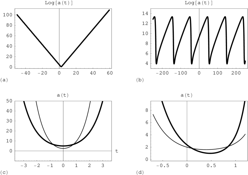
Figure 5: Selected plots of the scale factor of the FRW universe in the NC-frame realization (thick lines) in contrast with C-frame realization (thin lines). $\left(a\right):\theta=-0.9,$ $\mu=0.6,$ $\nu=1.78$, $\xi_{0}=1.7,$ and$\ \eta_{0}=4.5$. $\left(b\right):\theta=0.1,$ $\mu=0.3,$ $\nu=-0.3$, $\xi_{0}=1,$ and$\ \eta_{0}=10.$ $\left(c\right):\theta=1,$ $\xi_{0}=5,$ and$\ \eta_{0}=0.$ $\left(d\right):\theta=-1.5,$ $\alpha=1.5$, $a_{0}=2,$ and$\ \eta_{0}=0.$

VII Discussion

In this work, we carried out an investigation into the role of noncommutative geometry in the cosmological scenario by introducing a noncommutative deformation in the algebra of the minisuperspace variables along the same lines proposed in 15 and followed in 16 . As a cosmological model to carry out such an investigation, we chose a Friedman-Robertson-Walker universe with conformally coupled scalar field. A parallel was drawn between the realizations of noncommutativity in two possible frameworks for physical interpretation: the C-frame, where it manifest through $\theta$-dependent terms the Hamiltonian, and in the NC-frame, where it is manifest directly in the universe degrees of freedom.

The influence of noncommutativity in the universe evolution and its capability to remove cosmological singularities was investigated by means of a comparative study of the FRW model in four different versions: classical commutative, classical noncommutative, quantum commutative and quantum noncommutative. The confrontation between the classical and quantum versions was rendered easy by the Bohmian interpretation of quantum theory, which provided a common language for comparison through the quantum trajectory formalism. An extension of the Bohmian formulation to comprise noncommutative effects was previously proposed for the Kantowski-Sachs model in 16 . In our comparative study we have dealt with the noncommutative quantum model along the same lines. The “beable” mapping commonly employed in Bohmian quantum mechanics was extended to noncommutative quantum cosmology. In the commutative context, our formulation is reduced to the one proposed by Holland 20 in the minisuperspace approximation.

In the classical context, the main result of our investigation is that, contrary to the noncommutative Kantowski-Sachs model, for $\theta$ sufficiently large the noncommutative FRW can be non-singular. When $\left|\theta\right|\geq 1$, noncommutativity can give rise to bouncing universes in the NC- and C-frame realizations. The $\theta=\pm 1$ case is of particular interest since it reveals the capability noncommutativity has to mimic quantum effects under special conditions. The bouncing solutions that appear in both NC- and C-frame realizations [Eqs. (23) and (24)] can be mapped into the commutative quantum solution (55) with an appropriate identification of the integration constants. Therefore noncommutative classical quantum universe can be indistinguishable from a commutative quantum universe. Similar correspondences involving the noncommutative classical universe and other bouncing solutions of noncommutative quantum cosmology were described in section 6.

While in the classical context non-singular universe solutions can exist only in the noncommutative universe model and for $\left|\theta\right|\geq 1$, in the quantum context one may find non-singular universe solutions even in the commutative case. The qualitative behavior of the universe solutions in noncommutative quantum cosmology was discussed in section 4, where examples were presented that contain non-singular periodic solutions, non-singular solutions presenting one bounce, as well as non-singular solutions containing an infinite sequence of bounces enveloped by a larger bounce. When noncommutativity effects are turned on in the quantum scenario, they give rise to dynamical universes in situations where Bohmian quantum cosmology admits only static universes. One example is that of real wavefunctions, which in the noncommutative FRW model with a conformally coupled scalar field represent always non-singular bouncing universes. Noncommutativity effects can also induce a dynamical behavior yielding non-singular periodic universes in cases where the commutative counterpart is static and the noncommutative wavefunction is complex. An example was presented in section 6.

The investigation into the NC-C-frame correspondence revealed that, even in the classical context, the description of the universe evolution provided by these two possible scenarios for the realization of noncommutativity can differ radically. In section 3 we showed that for some values of the integration constants the universe can be non-singular in the NC-frame, while its C-frame counterpart is singular. An example of the drastic difference that can occur between the NC- and C-frame realizations was exhibited in that section for the case where $\theta=\pm 1$. It consists of a universe that is non-singular in the NC-frame and that has no correspondent in the C-frame, where it is at all times singular.

In the quantum context the distinction between the NC- and C-frame descriptions was shown to be as relevant as it is in the classical one. An example was worked out that discusses how a universe with large $a_{nc\min}$ in the NC-frame can correspond to two universes in the C-frame, one with large $a_{c\min}\simeq$ $a_{nc\min}$, and other with very small $a_{c\min}$. Such an interplay between small and large scale distances was previously reported in 22.3 , where it was interpreted as a sort of “IR-UV mixing”, in analogy with noncommutative field theory. Other examples involving the NC-C-frame correspondence were presented and solved numerically for the case $\left|\theta\right|<1$ and analytically for the case $\left|\theta\right|>1$. Again the case where $\theta=\pm 1$ provided an interesting example. When $\theta=\pm 1$ noncommutativity effects act to drop the kinetic term from the Wheeler-DeWitt equation. This justifies the poor and highly constrained dynamics found in this case. No matter what is the wavefunction in this case, if the initial conditions are non-singular the universe is non-singular and experiments a single bounce in both NC- and C-frame descriptions (Fig. $5c$).

In case noncommutativity of the minisuperspace variables has in fact played a role in the evolution of the primordial universe, as proposed in 15 , the study carried out in this work renders evident the need of an ontology in order to have a clear picture of the essential features of the noncommutative universe models. The correspondence between degrees of freedom in two different frames of realization is not sufficient to define the theory completely, which is only fixed by assuming one of them as the physical frame. This necessity seems not to be an exclusive feature of the cosmological model considered here, where the dramatic difference in the universe evolution can be attributed, in part, to the fact that the noncommutativity in question is that of the system’s degrees of freedom - the minisuperspace variables-. In the models where noncommutativity does not involve directly the system’s degrees of freedom, as the canonical noncommutative field theories that come from string theory 3 , the study of the correspondence between the NC- and C-frame descriptions is also a relevant subject. In the context of gauge theories, where the connection between the NC- and C- frames is via the Seiberg-Witten map, an investigation into the properties of the theory that have resemblance with gravity was carried out, e.g., in 6.5 , where the equivalence between spacetime translations and gauge transformations is shown to occur in the NC-frame. In the C-frame, on the other hand, where such an equivalence seems to be lost, noncommutative fields can be interpreted as ordinary theories immersed in a gravitational background generated by the gauge field, as shown in the interesting work by Rivelles 30 , and further in 31 .

References

- (1) R. J. Szabo, Phys. Rep. 378, 207 (2003).
- (2) M. R. Douglas and N.A. Nekrasov, Rev. Mod. Phys. 73, 977 (2002).
- (3) N. Seiberg and E. Witten, J. High Energy Phys. 09, 032 (1999).
- (4) S. Minwalla, M. Van Raamsdonk and N. Seiberg, J. High Energy Phys. 02, 020 (2000).
- (5) S. M. Carroll, J. A. Harvey, V.A. Kostelecky, C.D. Lane and T. Okamoto, Phys. Rev. Lett. 87, 141601 (2001); C. E. Carlson, C. D. Carone and R. F. Lebed, Phys. Lett. B 518, 201 (2001); Phys. Lett. B 549, 337 (2002); A. Anisimov, T. Banks, M. Dine and M. Graesser, Phys. Rev. D 65, 085032 (2002); J. M. Carmona, J. L. Cortés, J. Gamboa and F. Méndez, Phys. Lett. B 565, 222 (2003);
- (6) D. J. Gross and N. A. Nekrasov, J.High Energy Phys. 10, 021(2000); F. Lizzi, R.J. Szabo and A. Zampini, J. High Energy Phys. 08, 032 (2001).
- (7) J. M. Romero and J.A. Santiago, Cosmological Constant and Noncommutativity: A Newtonian Approach, hep-th/0310266.
- (8) R. Brandenberger and P.-M. Ho, Phys. Rev. D 66, 023517 (2002); Q.-G. Huang and M. Li, J. Cosmology Astroparticle Phys. 11, 001 (2003); J. High Energy Phys. 03, 014 (2003); “Power Spectra in Spacetime Noncommutative Inflation”, astro-ph/0311378; H. Kim, G. S. Lee and Y. S. Myung, “Noncommutative spacetime effect on the slow-roll period of inflation”, hep-th/0402018; H. Kim, G. S. Lee, H. W. Lee and Y. S. Myung,“Second-order corrections to noncommutative spacetime inflation”, hep-th/0402198; Y. S. Myung, “Cosmological parameters in the noncommutative inflation”, hep-th/0407066; Dao-jun Liu and Xin-zhou Li, “Cosmological perturbations and noncommutative tachyon inflation”, astro-ph/0402063; G. Calcagni,“Noncommutative models in patch cosmology”, hep-th/0406006; “ Consistency relations and degeneracies in (non)commutative patch inflation”, hep-ph/0406057; Rong-Gen Cai, Phys. Lett. B 593, 1 (2004); C.-S. Chu, B. R. Greene and G. Shiu, Mod. Phys. Lett. A 16, 2231 (2001); S. Tsujikawa, R. Maartens and R. Brandenberger, Phys. Lett. B 574, 141 (2003); H. Kim, G. S. Lee, H. W. Lee and Y. S. Myung, Second-order corrections to noncommutative spacetime inflation, hep-th/0402198; G. Calcagni and S. Tsujikawa, Observational constraints on patch inflation in noncommutative spacetime, astro-ph/0407543.
- (9) M. Maceda, J. Madore , P. Manousselis e G. Zoupanos, Eur. Phys. J. C 36, 529 (2004).
- (10) H. Garcia-Compeán, O. Obregón and C. Ramírez, Phys. Rev. Lett. 88, 161301 (2002).
- (11) G. D. Barbosa and N. Pinto Neto, “Noncommutative Geometry and Cosmology”, hep-th/0407111.
- (12) J. B. Hartle in :High energy Physics 1985, ed. M. J. Bowick and F. Gürsey (World Scientific, Singapore, 1986); J. Feinberg and Y. Peleg, Phys. Rev. D 52, 1988 (1995); M. Cavaglià, V. de Alfaro, and A, T. Filippov, Int J. Mod. Phys. A 10, 611 (1995).
- (13) J. A. de Barros, N. Pinto-Neto, and A. A. Sagioro-Leal, Gen. Rel. Grav. 32, 15 (2000).
- (14) D. Bohm, Phys. Rev. 85, 166 (1952); Phys. Rev. 85, 180 (1952).
- (15) D. Bohm, B. J. Hiley and P. N. Kaloyerou, Phys. Rep. 144, 349 (1987). D. Bohm, B. J. Hiley, The Undivided Universe: An Ontological Interpretation of Quantum Theory, London (Routledge & Kegan Paul, 1993);
- (16) S. Goldstein, Phys. Today, March (1998) 42; April (1998) 38.
- (17) J. S. Bell, Speakable and unspeakable in quantum mechanics, Cambridge University Press, Cambridge, 1993.
- (18) P. R. Holland, The Quantum Theory of Motion: An Account of the de Broglie-Bohm Causal Interpretation of Quantum Mechanics (Cambridge University Press, Cambridge, 1993).
- (19) D. Dürr. S. Goldstein, and N. Zanghì, J. Stat. Phys. 67, 843 (1992).
- (20) D. Dürr, S. Goldstein, N. Zanghì, “Bohmian Mechanics and the Meaning of the Wave Function”, “Experimental Metaphysics-Quantum Mechanical Studies in Honor of Abner Shimony,” ed. R.S.Cohen, M. Horne, and J. Stachel, Boston Studies in the Philosophy of Science (Kluwer, 1996) [quant-ph/9512031].
- (21) D. Dürr , S. Goldstein and N. Zanghì, “Bohmian Mechanics as the Foundation of Quantum Mechanics”, Contribution to “Bohmian Mechanics and Quantum Theory: An Appraisal,” edited by J.T. Cushing, A. Fine, S. Goldstein, Kluwer Academic Press.
- (22) V. Allori and N. Zanghì, “What is Bohmian Mechanics”, quant-ph/0112008.
- (23) H. Nikolic, “Covariant canonical quantization of fields and Bohmian mechanics”, hep-th/0407228; D. Durr, S. Goldstein, R. Tumulka, N. Zanghi, J. Phys. A 36, 4143 (2003); C. Colijn, E. R. Vrscay, Phys. Lett. A 300, 334 (2002); A. S. Sans, F. Borondo and S. Miret-Artés, J. Phys. Condens. Matter 14, 6109 (2002); D. Home and A. S. Majumdar, Found. Phys. 29, 721 (1999); L. Delle Site, Europhysics Letters 57, 20 (2002);. G. Gruebl, R. Moser, K. Rheinberger, J. Phys. A 34, 2753 (2001). Md. Manirul Ali, A. S. Majumdar and D. Homel, Phys. Lett. A 334, 61 (2002); E. Guay and L. Marchildon, J. Phys. A 36 5617 (2003); D. Dürr, S. Goldstein, S. Teufel and N. Zanghi, Physica A 279, 416 (2000);
- (24) J. Kowalski-Glikman and J. C. Vink, Class. Quant. Grav. 7, 901 (1990); Squires, Phys. Lett. A 162, 35 (1992); Y. V. Shtanov, Phys. Rev. D 54, 2564 (1996); R. Colistete Jr., J. C. Fabris, N. Pinto-Neto, Phys. Rev. D 62, 083507 (2000); F. Shojai, A. Shojai, J. High Energy Phys. 05, 037 (2001); Class. Quant. Grav. 21, 1 (2004); A. S. Sans, F. Borondo and S. Miret-Artés, J. Phys. Condens. Matter 14, 6109 (2002); W.-H. Huang, I.-C. Wang, “Quantum Perfect-Fluid Kaluza-Klein Cosmology”, gr-qc/0309042; J. Acacio de Barros and N. Pinto-Neto, Phys. Lett. A 241, 229 (1998); R. Colistete Jr., J. C. Fabris, N. Pinto-Neto, Phys. Rev. D 62, 083507 (2000); N. Pinto-Neto, E. S. Santini, Phys. Rev. D 59, 123517 (1999).
- (25) C. Kiefer, “Conceptual issues in quantum cosmology”, Lect. Notes Phys. 541 (2000) [gr-qc/9906100]; N. Pinto Neto, “Quantum Cosmology”, VIII Brazilian School of Cosmology and Gravitation (Editions Frontieres, Gif-sur-Yvette, 1996).
- (26) V. Faraoni, E. Gunzig and P. Nardone, Fund. Cosmic Phys. 20, 121 (1999).
- (27) G. D. Barbosa, J. High Energy Phys. 05, 024 (2003).
- (28) G. D. Barbosa and N. Pinto-Neto, Phys. Rev. D 69, 065014 (2004).
- (29) M. Chaichian, M. M. Sheikh-Jabbari and A. Tureanu, Phys. Rev. Lett. 86, 2716 (2001).
- (30) L. M. Campbell and L. J. Garay, Phys, Lett. B 254, 49 (1991); M. Cavaglià, Mod. Phys. Lett. A 9, 1897 (1994).
- (31) C. Simeone, Gen. Rel. Grav. 34, 1887 (2002).
- (32) A. Peres and D. R. Terno, Rev. Mod. Phys. 76, 93 (2004).
- (33) I. S. Gradshteyn and I. M. Ryzhik, Table of Integrals, Series and Products, Academic Press, San Diego, fourth edition.
- (34) V. O. Rivelles, Phys. Lett. B 558, 191 (2003).
- (35) Hyun Seok Yang, “Exact Seiberg-Witten Map and Induced Gravity from Noncommutativity”, hep-th/0402002.