hep-th/0407050

Sequences of Bubbles and Holes:

New Phases of Kaluza-Klein Black Holes

Henriette Elvang$\,{}^{1}$, Troels Harmark$\,{}^{2}$, Niels A. Obers$\,{}^{2}$

¹ Department of Physics, UCSB
Santa Barbara, CA 93106, USA

² The Niels Bohr Institute
Blegdamsvej 17, 2100 Copenhagen Ø, Denmark

elvang@physics.ucsb.edu, harmark@nbi.dk, obers@nbi.dk

We construct and analyze a large class of exact five- and six-dimensional regular and static solutions of the vacuum Einstein equations. These solutions describe sequences of Kaluza-Klein bubbles and black holes, placed alternately so that the black holes are held apart by the bubbles. Asymptotically the solutions are Minkowski-space times a circle, i.e. Kaluza-Klein space, so they are part of the $(\mu,n)$ phase diagram introduced in hep-th/0309116. In particular, they occupy a hitherto unexplored region of the phase diagram, since their relative tension exceeds that of the uniform black string. The solutions contain bubbles and black holes of various topologies, including six-dimensional black holes with ring topology $S^{3}\times S^{1}$ and tuboid topology $S^{2}\times S^{1}\times S^{1}$. The bubbles support the $S^{1}$’s of the horizons against gravitational collapse. We find two maps between solutions, one that relates five- and six-dimensional solutions, and another that relates solutions in the same dimension by interchanging bubbles and black holes. To illustrate the richness of the phase structure and the non-uniqueness in the $(\mu,n)$ phase diagram, we consider in detail particular examples of the general class of solutions.

1 Introduction

In four-dimensional vacuum gravity, a black hole in an asymptotically flat space-time is uniquely specified by the ADM mass and angular momentum measured at infinity [1, 2, 3, 4]. Uniqueness theorems [5, 6] for $D$-dimensional ($D>4$) asymptotically flat space-times state that the only static black holes in pure gravity are given by the Schwarzschild-Tangherlini black hole solutions [7]. However, in pure gravity there are no uniqueness theorems for non-static black holes with $D>4$, or for black holes in space-times with non-flat asymptotics. On the contrary, there are known cases of non-uniqueness. An explicit example of this occurs in five dimensions for stationary solutions in an asymptotically flat space-time: for a certain range of mass and angular momentum there exist both a rotating black hole with $S^{3}$ horizon [8] and rotating black rings with $S^{2}\times S^{1}$ horizons [9].

The topic of this paper is static black hole space-times that are asymptotically Minkowski space $\mathcal{M}^{d}$ times a circle $S^{1}$, in other words, we study static black holes in Kaluza-Klein theory. For brevity, we generally refer to these solutions as Kaluza-Klein black holes. Changing the boundary conditions from asymptotically flat space $\mathcal{M}^{d+1}$ to asymptotically $\mathcal{M}^{d}\times S^{1}$ opens up for a rich spectrum of black holes. As we shall see, the non-uniqueness of Kaluza-Klein black holes goes even further than for black holes in asymptotically flat space $\mathcal{M}^{d+1}$.

Much numerical [10, 11, 12, 13, 14, 15, 16] and analytical [17, 18, 19, 20, 21, 22, 23] work has been done to investigate the “phase space” of black hole solutions in Kaluza-Klein theory. Part of the motivation has been by the wish to reveal the endpoint for the classical evolution of the unstable uniform black string [24].

Recently, Refs. [19, 21] proposed a phase diagram as part of a program for classifying all black hole solutions of Kaluza-Klein theory. The input for the phase diagram consist of two physical parameters that are measured asymptotically: the dimensionless mass $\mu\propto M/L^{d-2}$, where $M$ is the ADM mass and $L$ is the proper length of the Kaluza-Klein circle at infinity, and the relative tension $n$ [19, 21, 25]. This is the tension per unit mass of a string winding the Kaluza-Klein circle. The $(\mu,n)$ phase diagram makes it possible to illustrate the different branches of solutions and exhibit their possible relationships. The main purpose of this paper is to construct and analyze a large class of exact five- and six-dimensional Kaluza-Klein black hole solutions occupying an hitherto unexplored region of the $(\mu,n)$ phase diagram.

In Kaluza-Klein space-times, it is well-known that there exist both uniform and non-uniform black strings with the same mass $\mu$ [26, 10, 11, 27, 13, 16] (see also [28, 29, 30]). There is also a family of topologically spherical black holes localized on the Kaluza-Klein circle [17, 14, 15, 22, 23]. These solutions, however, can be told apart at infinity, because they exist for different values of the relative tension $n$. We show in this paper that there is non-uniqueness of black holes in Kaluza-Klein theory, and we argue that for a certain open set of values of $\mu$ and $n$ there is even infinite non-uniqueness of Kaluza-Klein black holes. Infinite non-uniqueness has been seen before in [31] for black rings with dipole charges in asymptotically flat five-dimensional space. The solutions we present here are, on the contrary, solutions of pure gravity and the non-uniqueness involves regular space-times with multiple black holes. While some configurations have black holes whose horizons are topologically spheres, we also encounter black rings with horizon topologies $S^{d-2}\times S^{1}$ (for $d=4,5$), and in six dimensions a black tuboid with $S^{2}\times S^{1}\times S^{1}$ horizon.

A crucial feature of the black hole space-times studied in this paper is that they all involve Kaluza-Klein “bubbles of nothing”. Expanding Kaluza-Klein bubbles were first studied by Witten in [32] as the endstate of the semi-classical decay of the Kaluza-Klein vacuum $\mathcal{M}^{4}\times S^{1}$. The bubble is the minimal area surface that arises as the asymptotic $S^{1}$ smoothly shrinks to zero at a non-zero radius. The expanding Witten bubbles are non-static space-times with zero ADM mass. The Kaluza-Klein bubbles appearing in the solutions of this paper are on the other hand static with positive ADM mass. Kaluza-Klein bubbles will be reviewed early in the present paper.

The first solution combining a black hole and a Kaluza-Klein bubble was found by Emparan and Reall [33] as an example of an axisymmetric static space-time in the class of generalized Weyl solutions. Later Ref. [34] studied space-times with two black holes held apart by a Kaluza-Klein bubble and argued that the bubble balances the gravitational attraction between the two black holes, thus keeping the configuration in static equilibrium.

One natural question to ask is what the role of these solutions is in the phase diagram of Kaluza-Klein black holes. To address this issue we recall that one useful property of the $(\mu,n)$ phase diagram is that physical solutions lie in the region [19]

$$\mu\geq 0\ ,\ \ 0\leq n\leq d-2\,.$$ (1.1)

These bounds were derived using various energy theorems [35, 36, 19, 25]. However, so far only solutions in the lower region,

$$0\leq n\leq\frac{1}{d-2}\,,$$ (1.2)

have been discussed in connection to the phase diagram. This region includes the following three known branches:

• The uniform black string branch which has relative tension $n=1/(d-2)$ and hence bounds the region (1.2) from above. The uniform black string is classically unstable [24] for $\mu<\mu_{\mathrm{GL}}$, where $\mu_{\mathrm{GL}}$ is the Gregory-Laflamme mass, and it is believed to be stable for $\mu>\mu_{\mathrm{GL}}$.

• The non-uniform string branch [10, 11, 16] which emanates from the uniform string branch at $\mu=\mu_{\rm GL}$ and has decreasing $n$ and increasing (decreasing) $\mu$ for $4\leq d\leq 12$ ($d>12$).

• The black hole on cylinder branch [17, 22, 20, 19, 21, 14, 15, 23] which starts in the point $(\mu,n)=(0,0)$ and has increasing $n$ as $\mu$ increases. This is the branch of topologically spherical black holes localized on the Kaluza-Klein circle.

An obvious question is thus whether there are Kaluza-Klein black hole solutions occupying the upper region

$$\frac{1}{d-2}<n\leq d-2\,.$$ (1.3)

We will find in this paper that it is in fact the solutions involving Kaluza-Klein bubbles that occupy this region. A special point in the phase diagram is the static Kaluza-Klein bubble which corresponds to the single point $(\mu,n)=(\mu_{\rm b},d-2)$ in the phase diagram, where $\mu_{\rm b}$ is the dimensionless mass of the static Kaluza-Klein bubble.

More generally, we construct exact metrics for bubble-black hole configurations with $p$ bubbles and $q=p,p\pm 1$ black holes in $D=5,6$ dimensions. These are regular and static solutions of the vacuum Einstein equations, describing sequences of Kaluza-Klein bubbles and black holes placed alternately, e.g. for $(p,q)=(2,3)$ we have the sequence:

$$\mathrm{black~{}hole}~{}-~{}\mathrm{bubble}~{}-~{}\mathrm{black~{}hole}~{}-~{}\mathrm{bubble}~{}-~{}\mathrm{black~{}hole}\,.$$

We will call this class of solutions bubble-black hole sequences and refer to particular elements of this class as $(p,q)$ solutions. This large class of solutions, which was anticipated in Ref. [33], includes as particular cases the $(1,1)$, $(1,2)$ and $(2,1)$ solutions obtained and analyzed in [33, 34]. All of these solutions have $1/(d-2)<n<d-2$.

Besides their explicit construction, we present a comprehensive analysis of various aspects of these bubble-black hole sequences. This includes the regularity and topology of the Kaluza-Klein bubbles in the sequences, the topology of the event horizons, and general thermodynamical properties. An important feature is that the $(p,q)$ solutions are subject to constraints enforcing regularity, but this leaves $q$ independent dimensionless parameters allowing for instance the relative sizes of the black holes to vary. The existence of $q$ independent parameters in each $(p,q)$ solution is the reason for the large degree of non-uniqueness in the $(\mu,n)$ phase diagram, when considering bubble-black hole sequences.

The Kaluza-Klein bubbles play a key role in keeping these configurations in static equilibrium: not only do they balance the mutual attraction between the black holes, they also balance the gravitational self-attraction of black holes with non-trivial horizon topologies such as black rings. A different example of five-dimensional multi-black hole space-times based on the generalized Weyl ansatz was studied in Ref. [37]. Those solutions differ from ours in that they are asymptotically flat, and instead of bubbles, the black holes are held in static equilibrium by struts due to conical singularities.

For the simplest cases, we will plot the corresponding solution branches in the $(\mu,n)$ phase diagram, where they are seen to lie in the upper region (1.3). Moreover, these examples illustrate the richness of the phase structure and the non-uniqueness in the phase diagram.

The structure and main results of the paper are as follows. We introduce in Section 2 the $(\mu,n)$ phase diagram and explain how $\mu$ and $n$ are easily computed from the asymptotic behavior of the metric. We also briefly review the three known solution branches that occupy the region (1.2), i.e. the uniform and non-uniform black strings and the localized spherical black holes.

Section 3 provides a review of the static Kaluza-Klein bubble. In particular we review the argument that the static bubbles are classically unstable, and decay by either expanding or collapsing. We find a critical dimension $D=10$ below which the mass of the static bubble is smaller than the Gregory-Laflamme mass for the uniform black string. Hence, for $D\leq 10$ the endstate of the static bubble decay can be expected to be the endstate of the uniform black string, rather than the black string itself.

The bubble-black hole sequences are constructed using the general Weyl ansatz of [33]. We review this method in section 4, where we also write down metrics for the simplest Kaluza-Klein space-times and explain how to read of the asymptotic quantities using Weyl coordinates.

In Section 5 we construct the solution for the general bubble-black hole sequence in five dimensions. We analyze the constraints of regularity, the structure of the Kaluza-Klein bubbles, and the event horizons and their topology. We also compute the physical quantities relevant for the phase diagram and the thermodynamics. Section 6 provides a parallel construction and analysis for the six-dimensional bubble-black hole sequences.

It is shown that the five- and six-dimensional solutions are quite similar in structure and are in fact related by an explicit map. In particular, we find a map that relates the physical quantities, so that we can use it to obtain the phase diagram for the six-dimensional solutions from the five-dimensional one. This map is derived in Subsection 6.5.

For static space-times with more than one black hole horizon we can associate a temperature to each black hole by analytically continuing the solution to Euclidean space and performing the proper identifications needed to make the Euclidean solution regular where the horizon was located in the Lorentzian solution. The temperatures of the black holes need not be equal, and we derive a generalized Smarr formula that involves the temperature of each black hole. The Euclidean solution is regular everywhere only when all the temperatures are equal. It is always possible to choose the $q$ free parameters of the $(p,q)$ solution to give a one-parameter family of regular equal temperature solutions, which we shall denote by $(p,q)_{\mathfrak{t}}$.

We show in Section 7 that the equal temperature $(p,q)_{\mathfrak{t}}$ solutions are of special interest for two reasons: First, the two solutions, $(p,q)_{\mathfrak{t}}$ and $(q,p)_{\mathfrak{t}}$, are directly related by a double Wick rotation which effectively interchanges the time coordinate and the coordinate parameterizing the Kaluza-Klein circle. This provides a duality map under which bubbles and black holes are interchanged. The duality also implies an explicit map between the physical quantities of the solutions, in particular between the curves in the $(\mu,n)$ phase diagram.

Secondly, we show that for a given family of $(p,q)$ solutions, the equal temperature solution extremizes the entropy for fixed mass $\mu$ and fixed size of the Kaluza-Klein circle at infinity. For all explicit cases considered we find that the entropy is minimized for equal temperatures. This is a feature that is particular to black holes, independently of the presence of bubbles. As an analog, consider two Schwarzschild black holes very far apart. It is straightforward to see that for fixed total mass, the entropy of such a configuration is minimized when the black holes have the same radius (hence same temperature), while the maximal entropy configuration is the one where all the mass is located in a single black hole.

In Section 8 we consider in detail particular examples of the general five- and six-dimensional bubble-black hole sequences obtained in Sections 5-6. For these examples, we plot the various solution branches in the $(\mu,n)$ phase diagram and discuss the total entropy of the sequence as a function of the mass.

We find that the entropy of the $(1,1)$ solution is always lower than the entropy of the uniform black string of the same mass $\mu$. We expect that all other bubble-black hole sequences $(p,q)$ have entropy lower than the $(1,1)$ solution; we confirm this for all explicitly studied examples in Section 8. The physical reason to expect that all bubble-black hole sequences have lower entropy than a uniform string of same mass, is that some of the mass has gone into the bubble rather than the black holes, giving a smaller horizon area for the same mass.

As an appetizer, and to give a representative taste of the type of results we find for the phase diagram, we show in Figure 1 the phase diagram for six dimensions (the phase diagram for five dimensions is similar). Here we briefly summarize what is shown in the plot. The horizontal line $n=1/3$ is the uniform black string branch. This branch separates the diagram into two regions: $0\leq n\leq 1/3$ and $1/3<n\leq 3$.

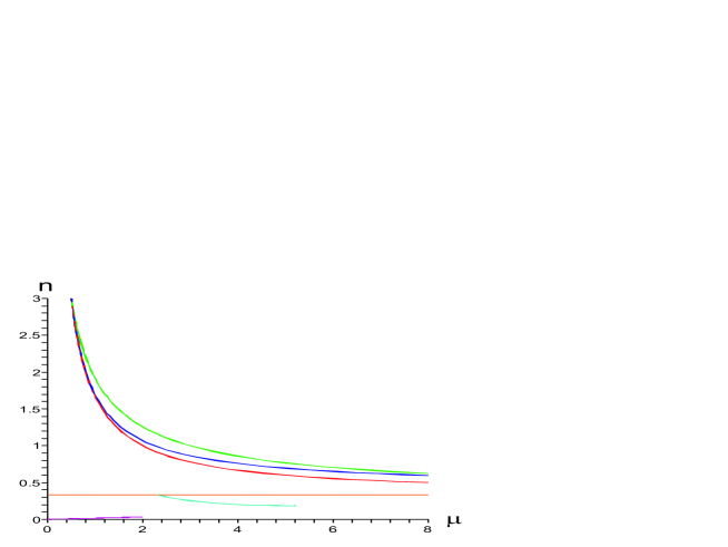
Figure 1: The $(\mu,n)$ phase diagram for six dimensions.

The region $0\leq n\leq 1/3$ has been the focus of many recent studies. The branch coming out of the uniform black string branch at $\mu_{\mathrm{GL}}\approx 2.3$ (the Gregory-Laflamme mass) is the non-uniform black string branch, which is reproduced here using numerical data courtesy Wiseman [11]. The curve starting at $(\mu,n)=(0,0)$ is the branch of spherical black holes localized on the Kaluza-Klein circle. Here we plot the slope of the first part of the branch using the analytical results for small black holes [22].

It is the region $1/3<n\leq 3$ that contains the bubble-black hole sequences. The top point of the curves in this region is the static bubble solution located at $(\mu,n)=(1/2,3)$. All $(p,q)$ solutions start out at this point and approach the uniform black string branch at $n=1/3$ as $\mu\to\infty$. The lowest lying of these curves is the $(p,q)=(1,1)$ solution with a single black ring (with horizon topology $S^{3}\times S^{1}$) supported by a single Kaluza-Klein bubble. There are also solutions lying “inside” the wedge bounded by the $(1,1)$ solution and the $(1,2)_{\mathfrak{t}}$ solution with one bubble balancing two equal size black rings with equal temperatures. The solutions in this wedge are all $(1,2)$ solutions where the two black rings are at different temperatures. We note that for any given $\mu>1/2$, the solutions in the wedge provide a continuous set of bubble-black hole sequences with the same mass. These solutions can be told apart since they have different values of $n$. But even specifying both $\mu$ and $n$ does not give a unique solution. Though not visible in the figure, the top curve crosses into the wedge of $(1,2)$ solutions at the value $\mu=117/10$. This curve is the one parameter family $(p,q)=(2,1)$ describing two equal-size Kaluza-Klein bubbles supporting a black tuboid, a black hole with horizon topology $S^{2}\times S^{1}\times S^{1}$.

We conclude in Section 9 with a discussion of our results and outlook for future developments. An appendix treats details of the analysis for the $(p,q)=(2,3)$ solution.

Notation

Throughout the paper we use $d$ to denote the space-time dimension of the Minkowski part of the metric. The space-times are asymptotically $\mathcal{M}^{d}\times S^{1}$, and we use $D=d+1$ for the dimension of the full space-time.

2 Review of the $(\mu,n)$ phase diagram

In [19, 21] a program was set forth to categorize — in higher-dimensional General Relativity — all static solutions of the vacuum Einstein equations that asymptote to $\mathcal{M}^{d}\times S^{1}$ for $d\geq 4$, with $\mathcal{M}^{d}$ being the $d$-dimensional Minkowski space-time. When an event horizon is present we call these solutions static neutral Kaluza-Klein black holes, since $\mathcal{M}^{d}\times S^{1}$ is a Kaluza-Klein type space-time. In this section we review the ideas and results of [19, 21] that are important for this paper.

The general idea is to define a “phase diagram” and plot in it the branches of different types of static Kaluza-Klein black holes. The physical parameters used in defining such a phase diagram should be measurable at asymptotic infinity. In [19, 20, 21] it was suggested that besides the proper length $L$ of the $S^{1}$ at infinity, the relevant physical parameters are the mass $M$ and the tension $\mathcal{T}$, which can be defined for any solution asymptoting to $\mathcal{M}^{d}\times S^{1}$. The tension $\mathcal{T}$ was defined in [38, 39, 19, 20, 25].

Let the $S^{1}$ be parameterized by the coordinate $\phi$, which we take to have period $L$. Define $(t,x^{1},...,x^{d-1})$ to be Cartesian coordinates for $\mathcal{M}^{d}$, so that the radial coordinate is $\rho=\sqrt{(x^{1})^{2}+\cdots+(x^{d-1})^{2}}$. We consider black holes localized in $\mathbb{R}^{d-1}$, so the asymptotic region is defined by $\rho\rightarrow\infty$, and we write the asymptotic behavior of the metric components $g_{tt}$ and $g_{\phi\phi}$ as

$$g_{tt}\simeq-1+\frac{c_{t}}{\rho^{d-3}}\ ,\ \ ~{}~{}~{}~{}g_{\phi\phi}\simeq 1+\frac{c_{\phi}}{\rho^{d-3}}$$ (2.1)

for $\rho\rightarrow\infty$. Note that we have chosen $\phi$ such that the period $L$ of $\phi$ is the proper length of the $S^{1}$ at infinity. It was shown in [19, 20, 25] that the ADM mass $M$ and the tension $\mathcal{T}$ along the $\phi$-direction can be computed from the asymptotic metric as

$$M=\frac{\Omega_{d-2}L}{16\pi G_{\rm N}}\left[(d-2)c_{t}-c_{\phi}\right]\ ,\ \ ~{}~{}~{}~{}\mathcal{T}=\frac{\Omega_{d-2}}{16\pi G_{\rm N}}\left[c_{t}-(d-2)c_{\phi}\right]\,,$$ (2.2)

where $\Omega_{m}=2\pi^{\frac{m+1}{2}}/\Gamma(\frac{m+1}{2})$ is the surface volume of the $m$-sphere.

Since for given $L$ we wish to compare solutions with the same mass, it is natural to normalize the mass with respect to $L$. We then work with the rescaled mass $\mu$ and the relative tension $n$, which are dimensionless quantities defined as

$$\mu=\frac{16\pi G_{\rm N}}{L^{d-2}}M=\frac{\Omega_{d-2}}{L^{d-3}}\left[(d-2)c_{t}-c_{\phi}\right]\ ,\ \ ~{}~{}n=\frac{\mathcal{T}L}{M}=\frac{c_{t}-(d-2)c_{\phi}}{(d-2)c_{t}-c_{\phi}}\,.$$ (2.3)

Not all values of $\mu$ and $n$ correspond to physically reasonable solutions. We have $\mu\geq 0$ from the Weak Energy Condition, and $n$ must satisfy the bounds [19]

$$0\leq n\leq d-2\,.$$ (2.4)

The lower bound comes from positivity of the tension [35, 36]. The upper bound is due to the Strong Energy Condition. There is a more physical way to understand the upper bound: for a solution with $n<d-2$ the gravitational force on a test particle at infinity is attractive, while it would be repulsive if $n>d-2$.

The aim of the work initiated in [19, 21] is to plot all static vacuum solutions that asymptote to $\mathcal{M}^{d}\times S^{1}$ in the $(\mu,n)$ phase diagram. In other words, we categorize all these solutions according to their physical parameters measured at asymptotic infinity. In this way one can get an overview of the possible solutions and one can for example see for a given mass $\mu$ what possible branches of solutions are available.

Previously only solutions with $0\leq n\leq 1/(d-2)$ have been considered for the $(\mu,n)$ phase diagram. We focus on that part of the phase diagram in the remainder of this section; the rest of the paper will discuss solutions in the $1/(d-2)<n\leq d-2$ region of the phase diagram.

According to our present knowledge, the solutions with $0\leq n\leq 1/(d-2)$ all have a local $SO(d-1)$ symmetry and two possible topologies for the event horizons: 1) $S^{d-1}$, which we call black holes on cylinders, and 2) $S^{d-2}\times S^{1}$, which we call black strings.

There are three known branches of solutions:

• Uniform black string branch. The metric for the uniform black string is constructed as the $d$-dimensional Schwarzschild metric times a circle:

  $$ds^{2}=-\left(1-\frac{\rho_{0}^{d-3}}{\rho^{d-3}}\right)dt^{2}+\left(1-\frac{\rho_{0}^{d-3}}{\rho^{d-3}}\right)^{-1}d\rho^{2}+\rho^{2}d\Omega_{d-2}^{2}+d\phi^{2}\ .$$ (2.5)

  We note that $c_{\phi}=0$, so by (2.3) a uniform black string has $n=1/(d-2)$. Gregory and Laflamme [24, 40] discovered that the uniform string is classically unstable for $\mu<\mu_{\rm GL}$, and the critical mass $\mu_{\rm GL}$ can be obtained numerically for each dimension $d$. In Table 1 we list the explicit values of $\mu_{\rm GL}$ for $d=4,\dots,14$. The uniform black strings are believed to be classically stable for $\mu>\mu_{\rm GL}$.

• The non-uniform black string branch. This branch was discovered in [27, 10]. For $d=4$ the beginning of the branch was studied in [10], and for $d=5$ a large piece of the branch was found numerically by Wiseman [11]. Recently, Sorkin [16] studied the non-uniform strings for general dimensions $d$. The non-uniform string branch starts at $\mu=\mu_{\rm GL}$ with $n=1/(d-2)$ in the uniform string branch and then it has decreasing $n$ and increasing $\mu$ for $d\leq 12$. Sorkin [16] found that for $d>12$ it has instead decreasing $n$ and $\mu$, which means that we have a critical dimension at $d=12$ where the physics of the non-uniform string branch changes. For $d\leq 12$ the non-uniform black string has lower entropy than the uniform black string with the same mass $\mu$, while for $d>12$ the non-uniform string has the higher entropy [16].

• The black hole on cylinder branch. This branch has been studied analytically in [17, 22, 20, 21, 23] (see also [19]) and numerically for $d=4$ in [14] and for $d=5$ in [15]. The branch starts in $(\mu,n)=(0,0)$ and has increasing $n$ and $\mu$. The first part of the branch is known analytically [22].

All three branches mentioned above can be described with the same ansatz for the metric. This ansatz was proposed in [17, 18], and proven in [12, 21].

In Figure 2 we display for $d=5$ the known solutions with $n\leq 1/3$ in the $(\mu,n)$ phase diagram. The non-uniform black string branch was drawn in [19] using the data of [11]. We included in the right part of Figure 2 the copies of the black hole on cylinder branch and the non-uniform string branch [28, 21].

     

Figure 2: Phase diagram for $d=5$ with $n\leq 1/3$. To the left we have the diagram without copies while we included the copies to the right.

For the temperature and entropy we use the rescaled temperature $\mathfrak{t}$ and entropy $\mathfrak{s}$ defined by

$$\mathfrak{t}=LT\ ,\ \ ~{}~{}~{}~{}\mathfrak{s}=\frac{16\pi G_{\rm N}}{L^{d-1}}S\,.$$ (2.6)

The dimensionless quantities $\mu$, $n$, $\mathfrak{t}$, and $\mathfrak{s}$ are connected through the Smarr formula [19, 20]

$$(d-1)\mathfrak{t}\,\mathfrak{s}=(d-2-n)\mu\,.$$ (2.7)

We also have the first law of thermodynamics [19, 20]

$$\delta\mu=\mathfrak{t}\,\delta\mathfrak{s}\,.$$ (2.8)

Using the two relations (2.7) and (2.8) one can pick a curve in the $(\mu,n)$ phase diagram and integrate the thermodynamics just from the points in the $(\mu,n)$ diagram alone [19]. In this way, the phase diagram contains the essential information about the thermodynamics of each branch. Note that for this argument we assumed that there was only one black hole present, so that there was only one temperature in the system. Later in this paper we present solutions with several disconnected event horizons, which can have different temperatures.

3 The static Kaluza-Klein bubble

Static Kaluza-Klein bubbles belong to the class of the solutions we wish to categorize in Kaluza-Klein theory, and they turn out to play a crucial role for the solutions in the $1/(d-2)<n\leq d-2$ region of the $(\mu,n)$ phase diagram. In this section, we introduce Kaluza-Klein bubbles and describe in detail the properties of static Kaluza-Klein bubbles.

Kaluza-Klein bubbles were discovered by Witten in [32], where it was explained that (in the absence of fundamental fermions) the Kaluza-Klein vacuum $\mathcal{M}^{4}\times S^{1}$ is semi-classically unstable to creation of expanding Kaluza-Klein bubbles. The expanding Kaluza-Klein bubble solutions can be obtained by a double Wick rotation of the 5D Schwarzschild solution and the resulting space-time is asymptotically $\mathcal{M}^{4}\times S^{1}$. The Kaluza-Klein bubble is located at the place where the $S^{1}$ direction smoothly closes off: this defines a minimal two-sphere in the space-time, i.e. a “bubble of nothing”. In this expanding Kaluza-Klein bubble solution the minimal two-sphere expands until all of the space-time is gone. Since it is not a static solution, the expanding Kaluza-Klein bubble is not in the class of solutions we consider for the $(\mu,n)$ phase diagram. We comment further on the expanding Kaluza-Klein bubble below.

However, there exist also static Kaluza-Klein bubbles. A $(d+1)$-dimensional static Kaluza-Klein bubble solution can be constructed by adding a trivial time-direction to the Euclidean section of a $d$-dimensional Schwarzschild black hole. This gives the metric

$$ds^{2}=-dt^{2}+\left(1-\frac{R^{d-3}}{\rho^{d-3}}\right)d\phi^{2}+\left(1-\frac{R^{d-3}}{\rho^{d-3}}\right)^{-1}d\rho^{2}+\rho^{2}d\Omega_{d-2}^{2}\ .$$ (3.1)

Clearly, this solution is static. It has a minimal $(d-2)$-sphere of radius $R$ located at $\rho=R$. To avoid a conical singularity at $\rho=R$, we need $\phi$ to be periodic with period

$$L=\frac{4\pi R}{d-3}\ .$$ (3.2)

With this choice of $L$ the Kaluza-Klein circle $\phi$ shrinks smoothly to zero as $\rho\to R$, and the location $\rho=R$ becomes a point with respect to the $\rho$ and $\phi$ directions. Around the location $\rho=R$ the space-time is locally of the form $\mathbb{R}\times\mathbb{R}^{2}\times S^{d-2}$, where $\mathbb{R}$ is the time, the two-plane is parameterized by $\rho$ and $\phi$, and the $S^{d-2}$ becomes the minimal $(d-2)$-sphere at $\rho=R$. Clearly, there are no boundaries at $\rho=R$ and no space-time for $\rho<R$, which is the reason for calling the Kaluza-Klein bubble a “bubble of nothing”. Note that the bubble space-time is a regular manifold with topology $\mathbb{R}\times\mathbb{R}^{2}\times S^{d-2}$, where the $S^{d-2}$ is non-contractible.

Due to the periodicity of $\phi$ we see that the static bubble (3.1) asymptotically (i.e. for $\rho\rightarrow\infty$) goes to $\mathcal{M}^{d}\times S^{1}$. Thus, it belongs to the class of solutions we are interested in, i.e. static pure gravity solutions that asymptote to $\mathcal{M}^{d}\times S^{1}$, and we can plot the solution in the $(\mu,n)$ phase diagram. Using (2.1) we read off $c_{t}=0$ and $c_{\phi}=-R^{d-3}$. From (2.3) and (3.2) we then find the dimensionless mass $\mu$ and the relative binding energy $n$ to be

$$\mu=\mu_{\rm b}\equiv\Omega_{d-2}\left(\frac{d-3}{4\pi}\right)^{d-3}\ ,\ \ ~{}~{}~{}~{}~{}~{}~{}n=d-2\,,$$ (3.3)

where we named this special value of $\mu$ as $\mu_{\rm b}$. Note that the static bubble only exists at one point in the $(\mu,n)$ diagram. This is because the relation between $L$ and $R$ in (3.2) means that once $L$ is chosen then all parameters are fixed. We note that since the static Kaluza-Klein bubble has $n=d-2$, it precisely saturates the upper bound in (2.4). Indeed, the Newtonian gravitational force on a test particle at infinity is zero.

The static Kaluza-Klein bubble is known to be classically unstable. This can be seen from the fact that the static bubble is the Euclidean section of the Schwarzschild black hole times a trivial time direction. The Euclidean flat space $\mathbb{R}^{3}\times S^{1}$ (hot flat space) is semi-classically unstable to nucleation of Schwarzschild black holes. This was shown by Gross, Perry, and Yaffe [41], who found that the Euclidean Lichnerowicz operator $\Delta_{\mathrm{E}}$ for the Euclidean section of the four dimensional Schwarzschild solution with mass $M$ has a negative eigenvalue: $\Delta_{\mathrm{E}}u_{ab}=\lambda u_{ab}$ with $\lambda=-0.19(GM)^{-2}$. The Lichnerowicz equation for the perturbations of the Lorentzian static bubble space-time is $\Delta_{\mathrm{L}}h_{ab}=0$ (in the transverse traceless gauge), so taking the ansatz $h_{ab}=u_{ab}\,e^{i\Omega t}$, the Lichnerowicz equation requires $\Omega^{2}=\lambda$, ie. $\Omega=\pm i\sqrt{-\lambda}$. So this is an instability mode of the static bubble, and the perturbation causes the bubble to either expand or collapse exponentially fast.

That the static Kaluza-Klein bubble is classically unstable poses the question: what does it decay to? We discuss this in the following.

Note first that the static bubble is massive, while the expanding Witten bubble obtained as the double Wick rotation of the Schwarzschild black hole is massless. Therefore the instability of the static bubble does not connect it directly to the Witten bubble. Furthermore, if $L$ is the size of the circle at infinity, the minimal radius of the Witten bubble is $\mathcal{R}=\frac{(d-2)}{4\pi}L$, and the radius of the static bubble is $R=\frac{d-3}{4\pi}L$. Therefore we have

$$R=\frac{d-3}{d-2}\mathcal{R}\,,$$ (3.4)

and this means that for given size of the Kaluza-Klein circle at infinity, the radius $R$ of the static Kaluza-Klein bubble is smaller than the minimal radius $\mathcal{R}$ of the expanding Kaluza-Klein bubble.

In the following, we discuss initial data describing massive bubbles that are initially expanding or collapsing, and we shall see that for given size of the Kaluza-Klein circle the initially expanding bubbles have larger radii than the static bubble, and collapsing bubbles have smaller radii. Presumably the collapse of a massive bubble results in a black hole or black string, so we shall also compare the mass $\mu_{\rm b}$ of the Kaluza-Klein bubble to the Gregory-Laflamme mass $\mu_{\mathrm{GL}}$.

Initial data for massive expanding and collapsing bubbles

We now consider a subclass of a more general family of initial data for five-dimensional vacuum bubbles found by Brill and Horowitz [42]. The metric on the initial surface is

$$ds^{2}=U(\rho)d\phi^{2}+U(\rho)^{-1}d\rho^{2}+\rho^{2}d\Omega_{2}^{2}$$ (3.5)

with $U(\rho)=1-2m/\rho-b/\rho^{2}$ for arbitrary parameters $m$ and $b$ satisfying $-m^{2}<b<\infty$. The bubble is located at the positive zero $\rho_{+}$ of $U$, $\rho_{+}=m+\sqrt{m^{2}+b}$, and by fixing the period of $\phi$ to be $L=2\pi\rho_{+}^{2}/(\rho_{+}-m)$ we avoid a conical singularity at $\rho=\rho_{+}$. The ADM mass is $G_{\rm N}M=\frac{1}{2}mL$, so

$$\mu=\frac{4m\sqrt{m^{2}+b}}{(m+\sqrt{m^{2}+b})^{2}}\,.$$ (3.6)

In the following we assume that $m>0$. In this case we find $0<\mu\leq 1$. Since this initial data exists for masses $\mu$ less than or equal to static bubble mass $\mu_{\rm b}=1$, it is not inconceivable that the evolution of this initial data can guide us about the possible endstates of the decay of the static Kaluza-Klein bubble.

For the initial data (3.5), Corley and Jacobson [43] showed that depending on the mass of the bubble and its size (or alternatively, the size of the $S^{1}$ at infinity), the bubbles are initially going to expand or collapse according to the initial acceleration of the bubble area which is given by

$$\ddot{A}=8\pi\left(1-\frac{2m}{\rho_{+}}\right)$$ (3.7)

(the derivatives are with respect to proper time). The relation (3.7) shows that for $b>0$ the bubble is initially expanding, but for $-m^{2}<b<0$ it is initially collapsing. We note that for $b=0$, we have $\mu=1$ and $\rho_{+}=2m$, so in this case the initial data describes an initially non-accelerating bubble. It is clear that (3.5) with $b=0$ is initial data for the static Kaluza-Klein bubble.

It may appear surprising that there are expanding as well as collapsing bubbles with the same mass $\mu$. The difference relies not on the mass, but in the radius of the bubble compared to the size of the circle at infinity. Consider for the initial data (3.5) the size of the bubble relative to the size $L$ of the Kaluza-Klein circle:

$$2\pi\frac{\rho_{+}}{L}=1-\frac{m}{\rho_{+}}\,.$$ (3.8)

For the static bubble ($b=0$), we have $\rho_{+}=2m$. Initially expanding bubbles ($b>0$) have $\rho_{+}>2m$ and initially collapsing bubbles ($-m^{2}<b<0$) have $\rho_{+}<2m$. So by (3.8) we see that bubbles that are bigger than the static bubble are going to expand and bubbles that are smaller are going to collapse.

In an interesting paper [44], Lehner and Sarbach recently studied numerically the evolution of the initial data (3.5) (as well as more general bubbles). They found that initially expanding bubbles continue to expand, and the smaller the mass of the bubble, the more rapidly the area of the bubble grows as a function of proper time. By studying such massive expanding bubbles, one can hope to learn about the endstate of the instability of perturbations of the static bubble.

The instability can also cause the static Kaluza-Klein bubble to collapse and thereby decay to another static solution, presumably one with an event horizon. The numerical results [44] show that for an initially collapsing massive bubble, the collapse continues until at some point an apparent horizon forms. A comparison of curvature invariants suggests that the resulting black hole is a uniform black string [44].

Is the endstate of the instability of the static Kaluza-Klein bubble then a black string? One would expect the endpoint of a classical evolution to be a classically stable configuration, so since the uniform black string is classically unstable for $\mu<\mu_{\mathrm{GL}}$ we must compare the mass of bubble $\mu_{\rm b}$ to the Gregory-Laflamme mass $\mu_{\mathrm{GL}}$.

Comparison of Kaluza-Klein bubble mass and Gregory-Laflamme mass

The mass $\mu_{\rm b}$ of the static Kaluza-Klein bubble is given in (3.3), and for $4\leq d\leq 9$ we can use the Gregory-Laflamme masses $\mu_{\mathrm{GL}}$ computed in [24, 40]. In Table 1 we list the approximate values of $\mu_{\rm GL}$ and $\mu_{\rm b}$. We see that for $4\leq d\leq 9$ the static bubble mass $\mu_{\rm b}$ is always lower than the Gregory-Laflamme mass $\mu_{\rm GL}$, so in the microcanonical ensemble the static Kaluza-Klein bubble cannot decay to the uniform black string branch but must decay to another branch of solutions, possibly the black hole on cylinder branch.

$d$	$4$	$5$	$6$	$7$	$8$	$9$	$10$	$11$	$12$	$13$	$14$
$\mu_{\rm GL}$	$3.52$	$2.31$	$1.74$	$1.19$	$0.79$	$0.55$	$0.37$	$0.26$	$0.18$	$0.12$	$0.08$
$\mu_{\rm b}$	$1$	$0.5$	$0.36$	$0.32$	$0.33$	$0.38$	$0.49$	$0.69$	$1.03$	$1.63$	$2.74$

Table 1: The mass $\mu_{\rm b}$ of the static Kaluza-Klein bubble compared to the critical masses $\mu_{\rm GL}$ for the Gregory-Laflamme instability. For $d\leq 9$, we use $\mu_{\rm GL}$ from [24, 40], and for $d>9$ we use the result of [16].

For higher $d$, we can use the results of [16]. Here it is found that the Gregory-Laflamme mass is $\mu_{\rm GL}=16.2\cdot 0.686^{d}$ for all $d$ to a good approximation. We have used this to plot in Figure 3 the static Kaluza-Klein bubble mass $\mu_{\rm b}$ versus the Gregory-Laflamme mass $\mu_{\rm GL}$, and also listed the approximate values for the dimensionless masses in Table 1. We see from Table 1 and Figure 3 that $\mu_{\rm b}$ is greater than $\mu_{\rm GL}$ for $d>9$. Therefore, for $d>9$ it is possible that the endpoint of the classical decay of the static Kaluza-Klein bubble is a uniform black string.

The fact that we have a critical dimension at $d=9$ ($D=10$) is interesting in view of the recent results of [16] showing that the non-uniform black string branch starts having decreasing $\mu$ as $n$ decreases for $d>12$, ie. with a critical dimension $d=12$ ($D=13$). Moreover, in Ref. [29] the critical dimension $d=9$ ($D=10$) appeared in studying the stability of the cone metric, as a model for the black hole-black string transition. It would therefore be interesting to examine whether there is any relation between these critical dimensions.

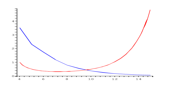
Figure 3: Plot of the static Kaluza-Klein bubble mass $\mu_{\rm b}$ and the Gregory-Laflamme mass $\mu_{\rm GL}$ versus $d$.

As we have seen, the classical instability of the static Kaluza-Klein bubble causes the bubble to either expand or collapse. For five-dimensional Kaluza-Klein space-times, there exists initial data [42] for massive bubbles that are initially expanding or collapsing [43], and numerical studies [44] shows us that there exist massive expanding bubbles and furthermore the numerical analysis indicates that contracting massive bubbles collapse to a black hole with an event horizon.

If the unstable mode of the static bubble preserves the translational invariance around the $S^{1}$-direction, the endstate of a collapsing bubble would be expected to be a uniform black string. Consider then more general perturbations causing the decay of the static bubble. For $d>9$ we found $\mu_{\rm b}>\mu_{\mathrm{GL}}$, so here it is possible that the static bubble decays to a stable uniform black string. Moreover, for $d>12$ the non-uniform strings have higher entropy than the uniform strings for a given $\mu$ [16], so here it is possible that a non-uniform string can be the endpoint of the bubble decay.

However, for $4\leq d\leq 9$, we have seen that the mass of the bubble lies in the range for which the uniform black string is classically unstable, and therefore we do not expect the uniform black string to be the endstate of the decay of the static bubble. It seems therefore plausable that for $4\leq d\leq 9$ the instability of the bubble develops inhomogeneities in the $S^{1}$-direction so that the likely endstate of the bubble decay is a black hole localized on the Kaluza-Klein circle (ie. a solution on the black hole on cylinder branch).

Summary

The static Kaluza-Klein bubble is massive and exists at a single point $(\mu_{\rm b},d-2)$ in the $(\mu,n)$ phase diagram. It is classically unstable and will either expand or collapse. In the latter case, the endstate is presumably an object with an event horizon. For $d\leq 9$ we have argued that it cannot be the uniform black string, but should be whatever is the endstate of the uniform black string.

It is important to emphasize that the static Kaluza-Klein bubble does not have any event horizon. This also means that it does not have entropy or temperature (i.e. the temperature is zero). However, in the following sections we discuss solutions in five and six dimensions with both Kaluza-Klein bubbles and event horizons present. In sections 5-6, we shall see that in the region $1/(d-2)<n<d-2$ of the $(\mu,n)$ phase diagram, all known solutions describe combinations of Kaluza-Klein bubbles and black hole event horizons, and for each value of $n$ in the range $1/(d-2)<n<d-2$ there exist continuous families of such solutions.

4 Generalized Weyl solutions

In this section we review the generalized Weyl solutions. We use this method in sections 5 and 6 to find exact solutions describing sequences of Kaluza-Klein bubbles and black holes. We examine the asymptotics of the generalized Weyl solutions and show how to read off the physical quantities from the asymptotic metric. Furthermore, as a warm-up to the following sections, we discuss the uniform black string and the static Kaluza-Klein bubble metrics in Weyl coordinates.

4.1 Review of generalized Weyl solutions

Emparan and Reall showed in [33] that for any $D$-dimensional static space-time with $D-1$ additional commuting orthogonal Killing vectors, i.e. with a total of $D-2$ commuting orthogonal Killing vectors, the metric can be written in the form

$$ds^{2}=-e^{2U_{1}}dt^{2}+\sum_{a=2}^{D-2}e^{2U_{a}}d\phi_{a}^{2}+e^{2\nu}(dr^{2}+dz^{2})\ .$$ (4.1)

where $U_{a}=U_{a}(r,z)$ and $\nu=\nu(r,z)$. For the metric (4.1) to be a solution of pure gravity, i.e. of the Einstein equations without matter, the potentials $U_{a}$, $a=1,\dots,D-2$, must obey

$$\left(\frac{\partial^{2}}{\partial r^{2}}+\frac{1}{r}\frac{\partial}{\partial r}+\frac{\partial^{2}}{\partial z^{2}}\right)U_{a}=0\ ,$$ (4.2)

and are therefore axisymmetric solutions of Laplace’s equation in a three-dimensional flat Euclidean space with metric

$$dr^{2}+r^{2}d\phi^{2}+dz^{2}\ .$$ (4.3)

The $U_{a}$ potentials are furthermore required to obey the constraint

$$\sum_{a=1}^{D-2}U_{a}=\log r\ .$$ (4.4)

Given the potentials $U_{a}$, $a=1,...,D-2$, the function $\nu=\nu(r,z)$ is determined, up to a constant, by the integrable system of differential equations

$$\partial_{r}\nu=-\frac{1}{2r}+\frac{r}{2}\sum_{a=1}^{D-2}\left[(\partial_{r}U_{a})^{2}-(\partial_{z}U_{a})^{2}\right]\ ,\ \ \partial_{z}\nu=r\sum_{a=1}^{D-2}\partial_{r}U_{a}\partial_{z}U_{a}\ .$$ (4.5)

Therefore, we can find solutions to the Einstein equations by first solving the Laplace equations (4.2) for the potentials $U_{a}$, $a=1,...,D-2$, subject to the constraint (4.4), and subsequently solve (4.5) to find $\nu$.

In four dimensions this method of finding static axisymmetric solutions was pioneered by Weyl in [45]. Emparan and Reall then generalized Weyl’s results to higher dimensions in [33]. We refer therefore to solutions of the kind described above as generalized Weyl solutions.

In general, sources for the $U_{a}$ potentials at $r>0$ lead to naked singularities, so we consider only sources at $r=0$. The location $r=0$ corresponds to a straight line in the unphysical three-dimensional space with metric (4.3) mentioned above. The constraint (4.4) then means that the total sum of the potentials is equivalent to the potential of an infinitely long rod of zero thickness lying along the $z$-axis at $r=0$. In the unphysical three-dimensional space (4.3), this infinite rod has mass $1/2$ per unit length, with Newton’s constant in this space set to one. We demand furthermore that for a given value of $z$ there is only one rod, except in isolated points. Thus, we build solutions by combining rods of mass $1/2$ per unit length for the different $U_{a}$ potentials under the restrictions that the rods do not overlap and that they add up to the infinite rod.

We use here and in the following the notation that $[z_{1},z_{2}]$ denotes a rod from $z=z_{1}$ to $z=z_{2}$.

We now review which rod sources to use for the potentials $U_{a}$ to write familiar static axisymmetric solutions in the generalized Weyl form:

Figure 4: Rod configurations for the four-dimensional (left) and five-dimensional (right) Schwarzschild black holes. The ends of the figures are supposed to represent $z=\pm\infty$, so that the semi-infinite rods for $U_{2}$ and $U_{3}$ extend all the way out to infinity.

• $D=4$ Minkowski space. No source for the $U_{1}$-potential of the $t$-direction, but an infinite rod $[-\infty,\infty]$ for the potential $U_{2}$ of the $\phi_{2}$-direction.

• A $D=4$ Schwarzschild black hole. A finite rod $[-\alpha,\alpha]$ for the potential $U_{1}$ of the $t$-direction, and two semi-infinite rods $[-\infty,-\alpha]$ and $[\alpha,\infty]$ for the potential $U_{2}$ of the $\phi_{2}$-direction. This is illustrated in the left part of Figure 4. Here $\alpha=G_{\rm N}M$ with $M$ being the mass of the black hole and $G_{\rm N}$ the four-dimensional Newton’s constant.

• $D=5$ Minkowski space. Two semi-infinite rods, one rod $[-\infty,0]$ for the potential $U_{2}$ in the $\phi_{2}$-direction, and the other rod $[0,\infty]$ for the potential $U_{3}$ for the $\phi_{3}$-direction. No sources for the potential $U_{1}$.

• A $D=5$ Schwarzschild black hole. The rod configuration is illustrated in the right part of Figure 4. It consists of a finite rod $[-\alpha,\alpha]$ for the potential $U_{1}$ in the $t$-direction, a semi-infinite rod $[-\infty,-\alpha]$ for $U_{2}$ of $\phi_{2}$-direction, and another semi-infinite rod $[\alpha,\infty]$ for $U_{3}$ of the $\phi_{3}$-direction. Here $\alpha=\frac{2}{3\pi}G_{\rm N}M$ with $M$ being the mass of the black hole and $G_{\rm N}$ the five-dimensional Newton’s constant.

Furthermore, we review in detail particular solutions that are crucial to this paper in Section 4.2.

As will become clearer in the following we have, for our purposes at least, the rule of thumb that a semi-infinite or infinite rod gives rise to a rotational axis (so that the corresponding coordinate becomes an angle in the metric), a finite rod in the time-direction $t$ gives rise to an event horizon, while a finite rod in the spatial directions results in a static Kaluza-Klein bubble.

4.2 Kaluza-Klein space-times as generalized Weyl solutions

In this section we show how we can write the five- and six-dimensional Kaluza-Klein space-times $\mathcal{M}^{4}\times S^{1}$ and $\mathcal{M}^{5}\times S^{1}$ as generalized Weyl solutions, and we explain how to read off the physical quantities for generalized Weyl solutions asymptoting to these space-times. We furthermore describe the uniform black string branch and the static Kaluza-Klein bubbles in five and six dimensions, since this clarifies our use of the generalized Weyl solution technique, and also since these solutions will be the building-blocks of the solutions presented below. We begin in five dimensions and then move on to six dimensions.

Five-dimensional Kaluza-Klein space-time $\mathcal{M}^{4}\times S^{1}$ and asymptoting solutions

For $D=5$ we have the generalized Weyl ansatz Eq. (4.1) which we write as

$$ds^{2}=-e^{2U_{1}}dt^{2}+e^{2U_{2}}d\phi^{2}+e^{2U_{3}}d\psi^{2}+e^{2\nu}(dr^{2}+dz^{2})\ .$$ (4.6)

Notice that we have renamed $\phi_{2}=\phi$ and $\phi_{3}=\psi$.

We begin by describing the $D=5$ Kaluza-Klein space-time $\mathcal{M}^{4}\times S^{1}$ as a generalized Weyl solution. This corresponds to the potentials

$$e^{2U_{1}}=1\ ,\ \ e^{2U_{2}}=1\ ,\ \ e^{2U_{3}}=r^{2}\ .$$ (4.7)

We see that this is an infinitely long rod $[-\infty,\infty]$ for the $U_{3}$ potential, i.e. in the $\psi$-direction. Note that $e^{2\nu}=1$ as can be checked from (4.5). Making the coordinate transformation

$$r=\rho\sin\theta\ ,\ \ z=\rho\cos\theta\ ,$$ (4.8)

we get four-dimensional Minkowski-space in spherical coordinates times a circle

$$ds^{2}=-dt^{2}+d\rho^{2}+\rho^{2}\left(d\theta^{2}+\sin^{2}\theta d\psi^{2}\right)+d\phi^{2}\ .$$ (4.9)

We see that $\phi$ is the circle direction which we take to be periodic with period $L$.

We now consider generalized Weyl solutions that asymptote to the five-dimensional Kaluza-Klein space-time $\mathcal{M}^{4}\times S^{1}$. The asymptotic region of a generalized Weyl solution is the region $\sqrt{r^{2}+z^{2}}\rightarrow\infty$.

In Section 2 we explained how to read off the rescaled mass $\mu$ and the relative tension $n$ for static solutions asymptoting to the five-dimensional Kaluza-Klein space-times $\mathcal{M}^{4}\times S^{1}$. From (2.3) we see that we need to read off $c_{t}$, $c_{\phi}$, and $L$ in order to find $\mu$ and $n$. While the circumference $L$ is clearly the period of $\phi$ we can read off $c_{t}$ and $c_{\phi}$ from the potentials $U_{1}$ and $U_{2}$ as

$$e^{2U_{1}}=1-\frac{c_{t}}{\sqrt{r^{2}+z^{2}}}+\mathcal{O}\left(\frac{1}{r^{2}+z^{2}}\right)\ ,\ \ e^{2U_{2}}=1+\frac{c_{\phi}}{\sqrt{r^{2}+z^{2}}}+\mathcal{O}\left(\frac{1}{r^{2}+z^{2}}\right)\ ,$$ (4.10)

for $\sqrt{r^{2}+z^{2}}\rightarrow\infty$. Using this in (2.3) with $d=4$ then gives $\mu$ and $n$.

Uniform black string and static Kaluza-Klein bubble in $\mathcal{M}^{4}\times S^{1}$

In Section 2 we reviewed the uniform black string in $\mathcal{M}^{d}\times S^{1}$, in particular the metric was given in (2.5). The five-dimensional uniform black string metric ($d=4$) can be written in Weyl coordinates by choosing the potentials

$$e^{2U_{1}}=\frac{R_{+}-\zeta_{+}}{R_{-}-\zeta_{-}}\ ,\ \ e^{2U_{2}}=1\ ,\ \ e^{2U_{3}}=(R_{+}+\zeta_{+})(R_{-}-\zeta_{-})\ ,$$ (4.11)

with

$$\zeta_{\pm}=z\pm\alpha\ ,\ \ R_{\pm}=\sqrt{r^{2}+(\zeta_{\pm})^{2}}\ .$$ (4.12)

This means that we have a finite rod $[-\alpha,\alpha]$ for the potential $U_{1}$ of the $t$-direction, no rod sources for the $U_{2}$ potential of the $\phi$-direction, and two semi-infinite rods $[-\infty,-\alpha]$ and $[\alpha,\infty]$ for the potential $U_{3}$ of the $\psi$-direction. We have depicted this rod configuration in the left part of Figure 5. Using (4.10) we see that $c_{t}=2\alpha$ and $c_{\phi}=0$. We have

$$e^{2\nu}=\frac{R_{+}R_{-}+\zeta_{+}\zeta_{-}+r^{2}}{2R_{+}R_{-}}\frac{R_{-}-\zeta_{-}}{R_{+}-\zeta_{+}}\ ,$$ (4.13)

as can be checked using (4.5). If we make the coordinate transformation

$$r=\rho\sqrt{1-\frac{2\alpha}{\rho}}\sin\theta\ ,\ \ z=(\rho-\alpha)\cos\theta\ ,$$ (4.14)

and set $\rho_{0}=2\alpha$ we get back the metric (2.5) for the uniform black string with $d=4$, which explicitly exhibits the $SO(3)$ spherical symmetry.

To get instead a static Kaluza-Klein bubble as a generalized Weyl solution we can make a double Wick rotation of the $t$ and $\phi$ directions. This gives the potentials

$$e^{2U_{1}}=1\ ,\ \ e^{2U_{2}}=\frac{R_{+}-\zeta_{+}}{R_{-}-\zeta_{-}}\ ,\ \ e^{2U_{3}}=(R_{+}+\zeta_{+})(R_{-}-\zeta_{-})\ ,$$ (4.15)

with $\zeta_{\pm}$ and $R_{\pm}$ given by (4.12). This means that we have two semi-infinite rods $[-\infty,-\alpha]$ and $[\alpha,\infty]$ in the $\psi$-direction and a finite rod $[-\alpha,\alpha]$ in the $\phi$-direction. We have depicted this rod-configuration in the right half of Figure 5. The function $\nu(r,z)$ is again given by (4.13). To avoid a conical singularity at $r\to 0$ for $|z|<\alpha$, where the orbit of $\partial_{\phi}$ shrinks to zero, we need to fix the period of $\phi$ to be $L=8\pi\alpha$. Using (4.10) we see that $c_{t}=0$ and $c_{\phi}=-2\alpha$, so $\mu=1$ and $n=2$ by Eq. (2.3). If we make the coordinate transformation (4.14) we get the explicitly spherically symmetric metric (3.1) for the static Kaluza-Klein bubble metric with $d=4$.

Figure 5: Rod configurations for the uniform black string (left) and the static Kaluza-Klein bubble (right) in five dimensions ($d=4$).

Six-dimensional Kaluza-Klein space-time $\mathcal{M}^{5}\times S^{1}$ and asymptoting solutions

For $D=6$ we have the generalized Weyl ansatz Eq. (4.1) which we write as

$$ds^{2}=-e^{2U_{1}}dt^{2}+e^{2U_{2}}d\phi^{2}+e^{2U_{3}}d\psi^{2}+e^{2U_{4}}d\chi^{2}+e^{2\nu}(dr^{2}+dz^{2})\ .$$ (4.16)

Notice that we have renamed $\phi_{2}=\phi$, $\phi_{3}=\psi$ and $\phi_{4}=\chi$.

Written as a generalized Weyl solution the $D=6$ Kaluza-Klein space-time $\mathcal{M}^{5}\times S^{1}$ corresponds to the potentials

$$e^{2U_{1}}=1\ ,\ \ e^{2U_{2}}=1\ ,\ \ e^{2U_{3}}=\sqrt{r^{2}+z^{2}}+z\ ,\ \ e^{2U_{4}}=\sqrt{r^{2}+z^{2}}-z\ .$$ (4.17)

We see that this is a semi-infinite rod $[-\infty,0]$ sourcing the potential for the $\psi$-direction and a semi-infinite rod $[0,\infty]$ for the potential for the $\chi$-direction. We have

$$e^{2\nu}=\frac{1}{2\sqrt{r^{2}+z^{2}}}\ ,$$ (4.18)

as can be verified using (4.5). Making the coordinate transformation

$$r=\frac{1}{2}\rho^{2}\sin 2\theta\ ,\ \ z=\frac{1}{2}\rho^{2}\cos 2\theta\ ,$$ (4.19)

where $\theta\in[0,\frac{\pi}{2}]$, we see that we get five-dimensional Minkowski-space in spheroidal coordinates times a circle

$$ds^{2}=-dt^{2}+d\rho^{2}+\rho^{2}\left(d\theta^{2}+\cos^{2}\theta d\psi^{2}+\sin^{2}\theta d\chi^{2}\right)+d\phi^{2}\ .$$ (4.20)

We consider now six-dimensional generalized Weyl solutions that asymptote to $\mathcal{M}^{5}\times S^{1}$. We can read off $c_{t}$ and $c_{\phi}$ from the asymptotics of the potentials since we have

$$e^{2U_{1}}=1-\frac{\frac{1}{2}c_{t}}{\sqrt{r^{2}+z^{2}}}+\mathcal{O}\left(\frac{1}{r^{2}+z^{2}}\right)\ ,\ \ e^{2U_{2}}=1+\frac{\frac{1}{2}c_{\phi}}{\sqrt{r^{2}+z^{2}}}+\mathcal{O}\left(\frac{1}{r^{2}+z^{2}}\right)\ ,$$ (4.21)

for $\sqrt{r^{2}+z^{2}}\rightarrow\infty$. Using this with (2.3) for $d=5$ we get $\mu$ and $n$.

Uniform black string and static Kaluza-Klein bubble in $\mathcal{M}^{5}\times S^{1}$

The $D=6$ uniform black string as a generalized Weyl solution has the potentials

$$e^{2U_{1}}=\frac{R_{+}-\zeta_{+}}{R_{-}-\zeta_{-}}\ ,\ \ e^{2U_{2}}=1\ ,\ \ e^{2U_{3}}=R_{+}+\zeta_{+}\ ,\ \ e^{2U_{4}}=R_{-}-\zeta_{-}\ ,$$ (4.22)

with

$$\zeta_{\pm}=z\pm\alpha\ ,\ \ R_{\pm}=\sqrt{r^{2}+(\zeta_{\pm})^{2}}\ .$$ (4.23)

The source configuration for the potentials $U_{a}$ are therefore a finite rod $[-\alpha,\alpha]$ for $U_{1}$, no source the potential $U_{2}$, a semi-infinite rod $[-\infty,-\alpha]$ for $U_{3}$, and a semi-infinite rod $[\alpha,\infty]$ for $U_{4}$. We have depicted this rod configuration in the left half of Figure 6. Using (4.21) we see that $c_{t}=\alpha$ and $c_{\phi}=0$. The function $\nu$ is given by

$$e^{2\nu}=\frac{\sqrt{R_{+}R_{-}+\zeta_{+}\zeta_{-}+r^{2}}}{2\sqrt{2}R_{+}R_{-}}\sqrt{\frac{R_{-}-\zeta_{-}}{R_{+}-\zeta_{+}}}\ ,$$ (4.24)

as can be checked using (4.5). Notice Eq. (4.24) reduces to Eq. (4.18) for $\alpha=0$. If we set $\rho_{0}=2\sqrt{\alpha}$ and make the coordinate transformation

$$r=\frac{1}{2}\rho^{2}\sqrt{1-\frac{4\alpha}{\rho^{2}}}\sin 2\theta\ ,\ \ z=\frac{1}{2}\rho^{2}\left(1-\frac{2\alpha}{\rho^{2}}\right)\cos 2\theta\ ,$$ (4.25)

with $\theta\in[0,\frac{\pi}{2}]$, we get the metric (2.5) for the $d=5$ uniform black string metric, which explicitly exhibits the $SO(4)$ spherical symmetry.

If we make a double Wick rotation of the $t$ and $\phi$-directions we get the $D=6$ static Kaluza-Klein bubble. This corresponds to the potentials

$$e^{2U_{1}}=1\ ,\ \ e^{2U_{2}}=\frac{R_{+}-\zeta_{+}}{R_{-}-\zeta_{-}}\ ,\ \ e^{2U_{3}}=R_{+}+\zeta_{+}\ ,\ \ e^{2U_{4}}=R_{-}-\zeta_{-}\ ,$$ (4.26)

This means we have no rod sources for $U_{1}$, a finite rod $[-\alpha,\alpha]$ for $U_{2}$, a semi-infinite rod $[-\infty,-\alpha]$ for $U_{3}$, and a semi-infinite rod $[\alpha,\infty]$ for $U_{4}$. We have depicted this rod-configuration in the right part of Figure 6. The function $\nu(r,z)$ is again given by (4.24). We need $L=2\pi\sqrt{\alpha}$ to avoid a conical singularity at $\rho\to 0$ for $|z|<\alpha$. Using (4.21) we see that $c_{t}=0$ and $c_{\phi}=-\alpha$, so $\mu=1/2$ and $n=3$ by Eq. (2.3). If we make the coordinate transformation (4.25) we get the explicitly spherically symmetric metric (3.1) for the static Kaluza-Klein bubble metric with $d=5$.

Figure 6: Rod configurations for the uniform black string (left) and the static Kaluza-Klein bubble (right) in six dimensions ($d=5$).

5 Five-dimensional bubble-black hole sequences

In this section we derive the metrics for bubble-black hole sequences in five dimensions, using the generalized Weyl construction reviewed above. We discuss some general aspects, such as regularity, topology of the Kaluza-Klein bubbles and event horizons, and the asymptotics of the solution. Specific cases as well as further general physical properties of these five-dimensional solutions are presented in Section 8.

5.1 Five dimensional $(p,q)$ solutions

In this section we construct five-dimensional solutions with $p$ static Kaluza-Klein bubbles and $q$ black holes. We use method of the generalized Weyl solutions reviewed in Section 4 to construct the solutions. This means we use the ansatz

$$ds^{2}=-e^{2U_{1}}dt^{2}+e^{2U_{2}}d\phi^{2}+e^{2U_{3}}d\psi^{2}+e^{2\nu}(dr^{2}+dz^{2})\ .$$ (5.1)

for the metric. The black holes and bubbles are placed alternately along the $z$-axis in the Weyl coordinates, like pearls on a string, for instance,

$$\mathrm{black~{}hole}~{}-~{}\mathrm{bubble}~{}-~{}\mathrm{black~{}hole}~{}-~{}\mathrm{bubble}~{}-\cdots-~{}\mathrm{black~{}hole}\,.$$

Two black holes (or two bubbles) cannot sit next to each other, so we have that $|p-q|\leq 1$.

To generate the black holes we place $q$ finite rods sourcing the potential $U_{1}$ for the $t$-direction. The static Kaluza-Klein bubbles are generated by placing $p$ finite rods sourcing the potential $U_{2}$ for the $\phi$-direction. The potential $U_{3}$ is then determined from the constraint (4.4).

For each Kaluza-Klein bubble in the solution we have a possible conical singularity which is absent only if the periodicity of $\phi$ is chosen appropriately. This gives rise to constraints which we examine in Section 5.2.

The period of $\psi$ is $2\pi$, since all the solutions asymptote to $D=5$ Kaluza-Klein space $\mathcal{M}^{4}\times S^{1}$ as described in Section 4.2. We study the asymptotics of the solutions in Section 5.4.

We introduce $N=p+q+1$ along with the set of numbers $a_{1}<a_{2}<\dots<a_{N}$, where $a_{i}$ denote the endpoints of the rods. In order to write the solution in a compact way, we follow [33] and introduce the following notation

$$\zeta_{i}=z-a_{i}\ ,\ \ R_{i}=\sqrt{r^{2}+\zeta_{i}^{2}}\ ,\ \ Y_{ij}=R_{i}R_{j}+\zeta_{i}\zeta_{j}+r^{2}$$ (5.2)

for $i,j=1,\dots,N$. We use this below to write down the solutions.

We now have three different cases: $p=q-1$, $p=q+1$ and $p=q$. We give the solutions for each of these cases in the following.

The case $p=q-1$

In this case the black hole-bubble sequence begins and ends with a black hole:

$$\mathrm{black~{}hole}~{}-~{}\mathrm{bubble}~{}-~{}\mathrm{black~{}hole}~{}-~{}\mathrm{bubble}~{}-\cdots-~{}\mathrm{black~{}hole}\,.$$

Note that $N=2p+2=2q$ so $N$ is even. The potentials are given by

$$\begin{array}[]{rccclcl}e^{2U_{1}}&=&\prod_{i=1}^{N}(R_{i}-\zeta_{i})^{(-1)^{i+1}}&=&\displaystyle\frac{R_{1}-\zeta_{1}}{R_{2}-\zeta_{2}}\frac{R_{3}-\zeta_{3}}{R_{4}-\zeta_{4}}\cdots\frac{R_{N-1}-\zeta_{N-1}}{R_{N}-\zeta_{N}}\,,\\[11.38109pt] e^{2U_{2}}&=&\prod_{i=2}^{N-1}(R_{i}-\zeta_{i})^{(-1)^{i}}&=&\displaystyle\frac{R_{2}-\zeta_{2}}{R_{3}-\zeta_{3}}\frac{R_{4}-\zeta_{4}}{R_{5}-\zeta_{5}}\cdots\frac{R_{N-2}-\zeta_{N-2}}{R_{N-1}-\zeta_{N-1}}\,,\\[11.38109pt] e^{2U_{3}}&=&(R_{1}+\zeta_{1})(R_{N}-\zeta_{N})\,.\end{array}$$ (5.3)

The corresponding rod configuration has $q$ finite rods $[a_{1},a_{2}]$, $[a_{3},a_{4}]$,…,$[a_{N-1},a_{N}]$ sourcing the potential $U_{1}$ (giving the $q$ black holes), and $p$ finite rods $[a_{2},a_{3}]$, $[a_{4},a_{5}]$,…,$[a_{N-2},a_{N-1}]$ sourcing $U_{2}$ (giving the $p$ Kaluza-Klein bubbles). The potential $U_{3}$ is sourced by two semi-infinite rods $[-\infty,a_{1}]$ and $[a_{N},\infty]$. We have depicted this rod-configuration in Figure 7.

Figure 7: Rod configurations for $p=q-1$ in five dimensions ($d=4$): The sequence begins and ends with a black hole.

One can now use (4.5) for the potentials in Eq. (5.3). This gives

$$e^{2\nu}=\frac{Y_{1N}}{2^{N/2}}\left(\prod_{i=1}^{N}\frac{1}{R_{i}}\right)\left(\prod_{2\leq i<j\leq N-1}Y_{ij}^{(-1)^{i+j+1}}\right)\sqrt{\prod_{i=2}^{N-1}\left(\frac{Y_{1i}}{Y_{iN}}\right)^{(-1)^{i}}}\,\frac{R_{N}-\zeta_{N}}{R_{1}-\zeta_{1}}\,.$$ (5.4)

For $(p,q)=(0,1)$ we see that we recover the uniform black string solution Eqs. (4.11)-(4.13) (setting $a_{1}=-\alpha$ and $a_{2}=\alpha$). For $(p,q)=(1,2)$ we get instead the solution with two black holes on a Kaluza-Klein bubble — this configuration was previously studied in [34]. The $(p,q)=(1,2)$ and $(2,3)$ solutions will be discussed in detail in Sections 8.2 and 8.3 respectively.

The case $p=q+1$

In this case the sequence begins and ends with a Kaluza-Klein bubble:

$$\mathrm{bubble}~{}-~{}\mathrm{black~{}hole}~{}-~{}\mathrm{bubble}~{}-~{}\mathrm{black~{}hole}-\cdots-~{}\mathrm{bubble}\,.$$

Note that $N=2q$ so $N$ is even. This case can be obtained from the previous case — where the solution started and ended with black holes — by a double Wick rotation of the $t$- and $\phi$-directions since the double Wick rotation interchanges the black holes and the bubbles. The potentials are given by

$$\begin{array}[]{rccclcl}e^{2U_{1}}&=&\prod_{i=2}^{N-1}(R_{i}-\zeta_{i})^{(-1)^{i}}&=&\displaystyle\frac{R_{2}-\zeta_{2}}{R_{3}-\zeta_{3}}\frac{R_{4}-\zeta_{4}}{R_{5}-\zeta_{5}}\cdots\frac{R_{N-2}-\zeta_{N-2}}{R_{N-1}-\zeta_{N-1}}\,,\\[11.38109pt] e^{2U_{2}}&=&\prod_{i=1}^{N}(R_{i}-\zeta_{i})^{(-1)^{i+1}}&=&\displaystyle\frac{R_{1}-\zeta_{1}}{R_{2}-\zeta_{2}}\frac{R_{3}-\zeta_{3}}{R_{4}-\zeta_{4}}\cdots\frac{R_{N-1}-\zeta_{N-1}}{R_{N}-\zeta_{N}}\,,\\[11.38109pt] e^{2U_{3}}&=&(R_{1}+\zeta_{1})(R_{N}-\zeta_{N})\,.\end{array}$$ (5.5)

The configuration thus has $q$ finite rods $[a_{2},a_{3}]$, $[a_{4},a_{5}]$,…,$[a_{N-2},a_{N-1}]$ sourcing the potential $U_{1}$ (giving the $q$ black holes), and $p$ finite rods $[a_{1},a_{2}]$, $[a_{3},a_{4}]$,…,$[a_{N-1},a_{N}]$ sourcing the potential $U_{2}$ (giving the $p$ Kaluza-Klein bubbles). The potential $U_{3}$ is sourced by two semi-infinite rods $[-\infty,a_{1}]$ and $[a_{N},\infty]$. We have depicted this rod-configuration in Figure 8. The function $\nu(r,z)$ is again given by (5.4). Note that one obtains Figure 8 from Figure 7 by interchanging the $t$- and $\phi$-directions. This is exactly the effect of the double Wick rotation mentioned above.

Figure 8: Rod configurations for $p=q+1$ in five dimensions ($d=4$): The sequence begins and ends with a Kaluza-Klein bubble.

For $(p,q)=(1,0)$ we regain the static Kaluza-Klein bubble solution given in Eqs. (4.15), (4.13) and (4.12) (putting $a_{1}=-\alpha$ and $a_{2}=\alpha$). The $(p,q)=(2,1)$ solution will be considered in detail in Section 8.2 and we also comment on the $(3,2)$ solution in Section 8.3.

The case $p=q$

In this case we start with a black hole and end with a Kaluza-Klein bubble:

$$\mathrm{black~{}hole}~{}-~{}\mathrm{bubble}~{}-~{}\mathrm{black~{}hole}-\cdots-~{}\mathrm{bubble}\,.$$

Note that $N=2p+1$ so $N$ is odd. We have the potentials

$$\begin{array}[]{rccclcl}e^{2U_{1}}&=&\prod_{i=1}^{N-1}(R_{i}-\zeta_{i})^{(-1)^{i+1}}&=&\displaystyle\frac{R_{1}-\zeta_{1}}{R_{2}-\zeta_{2}}\frac{R_{3}-\zeta_{3}}{R_{4}-\zeta_{4}}\cdots\frac{R_{N-2}-\zeta_{N-2}}{R_{N-1}-\zeta_{N-1}}\,,\\[11.38109pt] e^{2U_{2}}&=&\prod_{i=2}^{N}(R_{i}-\zeta_{i})^{(-1)^{i}}&=&\displaystyle\frac{R_{2}-\zeta_{2}}{R_{3}-\zeta_{3}}\frac{R_{4}-\zeta_{4}}{R_{5}-\zeta_{5}}\cdots\frac{R_{N-1}-\zeta_{N-1}}{R_{N}-\zeta_{N}}\,,\\[11.38109pt] e^{2U_{3}}&=&(R_{1}+\zeta_{1})(R_{N}-\zeta_{N})\,.\end{array}$$ (5.6)

Figure 9: Rod configurations for $p=q$ in five dimensions ($d=4$): This sequence begins with a black hole and ends with a Kaluza-Klein bubble.

The configuration thus has $q$ finite rods $[a_{1},a_{2}]$, $[a_{3},a_{4}]$,…,$[a_{N-2},a_{N-1}]$ sourcing the potential $U_{1}$ (giving the $q$ black holes), and $p$ finite rods $[a_{2},a_{3}]$, $[a_{4},a_{5}]$,…,$[a_{N-1},a_{N}]$ sourcing $U_{2}$ (giving the $p$ Kaluza-Klein bubbles). We have depicted this rod-configuration in Figure 9. From (4.5) one can find

$$e^{2\nu}=\frac{\sqrt{Y_{1N}}}{2^{N/2}}\left(\prod_{i=1}^{N}\frac{1}{R_{i}}\right)\left(\prod_{2\leq i<j\leq N-1}Y_{ij}^{(-1)^{i+j+1}}\right)\sqrt{\prod_{i=2}^{N-1}\left(Y_{1i}Y_{iN}\right)^{(-1)^{i}}}\,\frac{R_{N}-\zeta_{N}}{R_{1}-\zeta_{1}}\,.$$ (5.7)

Note that the solution (5.6)-(5.7) for the $p=q$ case that we consider here can formally be obtained from the $p=q-1$ case above. This is done by considering a configuration with $p+1$ black holes and $p$ bubbles and then setting $a_{N}=a_{N-1}$ where $N=2p+2$, and finally substituting $N-1\rightarrow N$.

For $(p,q)=(1,1)$ we get the solution with one black hole and one static Kaluza-Klein bubble studied previously in [33]. The $(p,q)=(1,1)$ solution will be considered in detail in Section 8.1, and we also comment on the $(2,2)$ solution in Section 8.3.

5.2 Regularity and topology of the Kaluza-Klein bubbles

We examine in this section the behavior of the solutions near the Kaluza-Klein bubbles. As stated above, for each of the $p$ Kaluza-Klein bubbles we have a possible conical singularity which is absent only if the periodicity of $\phi$ is chosen appropriately. Thus, in order to have a regular solution we have $p$ constraints that need to be obeyed. Below we write down these constraints for the solutions. We also examine the topology of the Kaluza-Klein bubbles by considering the metric on the bubbles.

We can count the number of free parameters characterizing a $(p,q)$ solution as follows. If we, as above, let $L$ be the circumference of the Kaluza-Klein circle parameterized by $\phi$, we see that for a given $L$ we have $p$ constraints on the $N=p+q+1$ parameters in order to have a regular solution. Therefore, we have $q+1$ parameters left by demanding regularity of the solution. By translational invariance we can disregard one of these, leaving now $q$ dimensionful parameters describing our solution (for a given circumference $L$). This means that we need $q$ dimensionless parameters to describe the space of regular $(p,q)$ solutions.

Before considering specific solutions we examine here the general features of how a solution behaves near a Kaluza-Klein bubble. Consider a rod $[z_{1},z_{2}]$ sourcing $U_{2}$, i.e. the potential for the $\phi$-direction. For $r\rightarrow 0$ with $z_{1}<z<z_{2}$ we have in general

$$ds^{2}=-g(z)dt^{2}+f(z)d\psi^{2}+\frac{1}{f(z)g(z)}\left[r^{2}d\phi^{2}+c^{2}(dr^{2}+dz^{2})\right]\,,$$ (5.8)

where $f(z)$ and $g(z)$ are functions and $c$ is a number. Clearly, this metric has a conical singularity at $r=0$, unless we take $\phi$ to have period $2\pi c$. Thus, we need that $L=2\pi c$. More generally, it is useful to write the regularity condition as

$$L=\Delta\phi=2\pi\lim_{r\rightarrow 0}\sqrt{\frac{r^{2}g_{rr}}{g_{\phi\phi}}}\,.$$ (5.9)

To see that the $(p,q)$ solutions reduce to the form (5.8) for $r\rightarrow 0$ near a bubble, one can use that for $r\rightarrow 0$ we have

$$\frac{R_{i}-\zeta_{i}}{R_{j}-\zeta_{j}}\simeq\left\{\begin{array}[]{ll}\frac{|\zeta_{i}|}{|\zeta_{j}|}&\mbox{for}~{}z<a_{i}<a_{j}\\[5.69054pt] \frac{r^{2}}{4|\zeta_{i}\zeta_{j}|}&\mbox{for}~{}a_{i}<z<a_{j}\\[5.69054pt] \frac{|\zeta_{j}|}{|\zeta_{i}|}&\mbox{for}~{}a_{i}<a_{j}<z\,,\end{array}\right.$$ (5.10)

and

$$Y_{ij}\simeq\left\{\begin{array}[]{ll}2|\zeta_{i}\zeta_{j}|&\mbox{ for }z<a_{i},a_{j}\mbox{ or }z>a_{i},a_{j}\\[2.84526pt] \frac{r^{2}(a_{j}-a_{i})^{2}}{2|\zeta_{i}\zeta_{j}|}&\mbox{ for }a_{i}<z<a_{j}\end{array}\right.$$ (5.11)

for the definitions (5.2). Using these formulas, one can obtain explicit expressions for $f(z)$, $g(z)$ and $c$ for each of the bubbles.

Note that we can read off the topology of the Kaluza-Klein bubbles from the metric (5.8). At $r=0$ and for fixed time $t$, we have the metric

$$(ds_{2})^{2}=f(z)d\psi^{2}+\frac{c^{2}}{f(z)g(z)}dz^{2}\,.$$ (5.12)

The topology of the Kaluza-Klein bubble as a two-dimensional surface is now determined from the behavior of $f(z)$ and $g(z)$ for $z\rightarrow z_{1},z_{2}$.

Since the bubble-rod is next to a rod either in the $U_{1}$ potential, corresponding to an event horizon, or the $U_{3}$ potential, if the bubble is at either end of the bubble-black hole sequence, we have that either $f(z)$ or $g(z)$ goes to zero for $z\rightarrow z_{1}$ (or for $z\rightarrow z_{2}$), but never both of them. We have therefore three different cases:

• The pure bubble space-time: there are no sources for the $U_{1}$ potential. This corresponds to the case $(p,q)=(1,0)$, which is the static bubble without any event horizon. In this case $f(z)$ goes to zero in both endpoints $z_{1}$ and $z_{2}$, so the bubble has the topology of a two-sphere $S^{2}$.

• The bubble sits between two event horizons. In this case $f(z)$ vanishes nowhere in the interval $[z_{1},z_{2}]$, so $\psi$ parameterizes a circle whose circumference varies with $z$ but never shrinks to zero size. The function $g(z)$ goes to zero at both endpoints $z_{1}$ and $z_{2}$. Since these are simple poles in the metric component $g_{zz}$ the $z$-coordinate parameterizes a finite interval $I$ of length

  $$s=c\int_{z_{1}}^{z_{2}}\big{[}f(z)g(z)\big{]}^{-1/2}dz\,,$$ (5.13)

  which we may think of as the proper distance between the two event horizons sitting on either side of the bubble. We conclude from the above that a bubble sitting between two event horizons is topologically a finite cylinder $S^{1}\times I$.

• The bubble is at either end of the bubble-black hole sequence. In terms of the rod configuration, there is a semi-infinite rod for the $U_{3}$ potential on one side of the bubble, say at $z=z_{1}$, and on the other side $z=z_{2}$ there is a finite rod for the $U_{1}$ potential (this gives rise to the event horizon sitting next to the bubble). In this case $f(z)$ goes to zero only at $z=z_{1}$, and $g(z)$ goes to zero only at $z=z_{2}$. Thus the $\psi$-circle shrinks smoothly to a point as $z\to z_{1}$, and the topology is therefore a disk $D$.

It should be noted that the bubble topologies determined above are inferred from the coordinate patch described by the metric (5.12). In the cases where an event horizon is present, the coordinates can be continued in a way analogous to that of the maximally extended Schwarzschild black hole. If the space-time has more than one event horizon, this extension is not uniquely given, but for the simplest bubble-black hole solutions we shall comment on this point when we consider examples of specific solutions in Section 8.

We now consider the constraints imposed on parameters of the solutions by the requirement of regularity. Again we consider the three cases $p=q-1$, $p=q+1$ and $p=q$ separately.

The case $p=q-1$

The sequence begins and ends with a black hole. From our above considerations, this means that each of the Kaluza-Klein bubbles has topology as a cylinder $S^{1}\times I$.

Using (5.9) together with (5.10)-(5.11), we see that the bubble corresponding to the $[a_{2k},a_{2k+1}]$ rod (sourcing $U_{2}$) requires $\phi$ to have the period

$$(\Delta\phi)_{k}=4\pi(a_{N}-a_{1})\prod_{i=2}^{2k}\prod_{j=2k+1}^{N-1}(a_{j}-a_{i})^{(-1)^{i+j+1}}\prod_{i=2}^{2k}[\sqrt{a_{N}-a_{i}}]^{(-1)^{i+1}}\prod_{i=2k+1}^{N-1}[\sqrt{a_{i}-a_{1}}]^{(-1)^{i}}$$ (5.14)

with $k=1,...,p$, in order to avoid a conical singularity on the bubble. Given the circumference $L$ of the Kaluza-Klein circle parameterized by $\phi$, we see then that we must require the $p$ constraints

$$L=(\Delta\phi)_{k}\,,~{}~{}~{}\mathrm{for~{}all}~{}k=1,\ldots,p$$ (5.15)

in order for the solution to be regular.

The case $p=q+1$

In this case we have Kaluza-Klein bubbles in both ends of the bubble-black hole sequence. If $p\geq 2$, this means that each of the two bubbles in the ends is topologically a disk $D$. Any other bubble in the solution has topology $S^{1}\times I$. If $p=1$ we have just one bubble with topology $S^{2}$.

Regularity of the $k$’th bubble, corresponding to the rod $[a_{2k-1},a_{2k}]$ sourcing $U_{2}$, requires $\phi$ to have period

$$(\Delta\phi)_{k}=4\pi(a_{N}-a_{1})\prod_{i=2}^{2k-1}\prod_{j=2k}^{N-1}(a_{j}-a_{i})^{(-1)^{i+j+1}}\prod_{i=2}^{2k-1}[\sqrt{a_{N}-a_{i}}]^{(-1)^{i+1}}\prod_{i=2k}^{N-1}[\sqrt{a_{i}-a_{1}}]^{(-1)^{i}}$$ (5.16)

with $k=1,...,p$. Given $L$, the $p$ constraints are then that $L=(\Delta\phi)_{k}$ for $k=1,...,p$.

The case $p=q$

In the left end of the sequence we have a black hole, while in the right end we have a bubble with topology as a disk $D$. Any other bubble in the solution has topology $S^{1}\times I$.

Regularity of the $k$’th bubble, corresponding to the rod $[a_{2k},a_{2k+1}]$ sourcing $U_{2}$, requires $\phi$ to have period

$$(\Delta\phi)_{k}=4\pi(a_{N}-a_{1})\prod_{i=2}^{2k}\prod_{j=2k+1}^{N}(a_{j}-a_{i})^{(-1)^{i+j+1}}\prod_{i=2}^{2k}[\sqrt{a_{N}-a_{i}}]^{(-1)^{i+1}}\prod_{i=2k+1}^{N}[\sqrt{a_{i}-a_{1}}]^{(-1)^{i}}$$ (5.17)

with $k=1,...,p$. Again, given $L$, the $p$ constraints are then that $L=(\Delta\phi)_{k}$ for $k=1,...,p$.

5.3 Event horizons, topology, thermodynamics and balance

In the above solutions we have $q$ finite rods sourcing $U_{1}$, where $U_{1}$ is the potential associated with the time-direction $t$. This gives $q$ event horizons. In the following we examine these event horizons, discuss their topologies and the associated temperatures and entropies.

We first consider the general features of how a solution behaves near an event horizon. Consider a rod $[z_{1},z_{2}]$ sourcing $U_{1}$, i.e. the potential for the time direction $t$. For $r\rightarrow 0$ with $z_{1}<z<z_{2}$ we have in general

$$ds^{2}=g(z)d\phi^{2}+f(z)d\psi^{2}+\frac{1}{f(z)g(z)}\left[-r^{2}dt^{2}+c^{2}(dr^{2}+dz^{2})\right]\,,$$ (5.18)

where $f(z)$ and $g(z)$ are functions and $c$ is a number. We see that we have an event horizon at $r=0$ since $g_{tt}$ goes to zero there, and the metric is otherwise regular at $r=0$. It is easy to see using (5.10)-(5.11) that the $(p,q)$ solutions reduce to the form (5.18) for $r\rightarrow 0$.

By Wick rotating the time-coordinate $t$ to the coordinate $\omega=it$, we can see that in the Euclidean section of the solution $\omega$ should have period $2\pi c$ in order to avoid a conical singularity at $r\to 0$. This means that the horizon has inverse temperature $2\pi c$. More generally, we can write this as

$$\beta=\frac{1}{T}=2\pi\lim_{r\rightarrow 0}\sqrt{\frac{r^{2}g_{rr}}{-g_{tt}}}\,.$$ (5.19)

We can also read off the topology of the event horizon. For $r=0$ and fixed $t$, we have the metric

$$(ds_{3})^{2}=g(z)d\phi^{2}+f(z)d\psi^{2}+\frac{c^{2}}{f(z)g(z)}dz^{2}\,.$$ (5.20)

This is the metric on the event horizon. Thus, we can find the topology of the event horizon as a three-dimensional surface by considering the behavior of the functions $f(z)$ and $g(z)$ for $z\rightarrow z_{1},z_{2}$. The analysis is similar to that of the bubble topology. There are three different cases:

• No bubbles present: this corresponds to the case $(p,q)=(0,1)$. Since there are no bubbles, $g(z)$ stays non-zero, and the $\phi$-coordinate parameterizes an $S^{1}$ which is just the Kaluza-Klein circle. The function $f(z)$ goes to zero at both endpoints $z_{1}$ and $z_{2}$, so $(z,\psi)$ parameterizes a two-sphere $S^{2}$. The topology of the event horizon is therefore $S^{2}\times S^{1}$, as expected since the solution $(p,q)=(0,1)$ is the uniform black string wrapping around the Kaluza-Klein circle.

• The event horizon has a bubble on both sides. In this case $g(z)$ goes to zero at both endpoints $z_{1}$ and $z_{2}$, so $(z,\phi)$ parameterizes an $S^{2}$. Since $f(z)$ stays non-zero we see that the $\psi$-direction corresponds to an $S^{1}$. The topology of the event horizon is therefore that of a black ring $S^{2}\times S^{1}$. Note that we call a black hole with horizon topology $S^{2}\times S^{1}$ a black ring if the $S^{1}$ is not topologically supported, i.e. if the $S^{1}$ direction is a contractible circle in the space-time and not the Kaluza-Klein circle parameterized by $\phi$. The $S^{1}$ of the black ring is supported by the Kaluza-Klein bubble against its gravitational self-attraction.

• The event horizon is at either end of the bubble-black hole sequence. In this case $f(z)$ goes to zero at one endpoint and $g(z)$ goes to zero at the other endpoint. It is not hard to see that the topology of the event horizon is a three-sphere $S^{3}$.

Note that none of the black holes are localized on the Kaluza-Klein circle.

We can read off the entropy of the event horizon by computing the area using the metric (5.20). Since the square-root of the determinant of the metric (5.20) is equal to $c$, we find the entropy to be

$$S=\frac{2\pi L(z_{2}-z_{1})c}{4G_{\rm N}}=\frac{2\pi L(z_{2}-z_{1})}{4G_{\rm N}}\lim_{r\rightarrow 0}\sqrt{\frac{r^{2}g_{rr}}{-g_{tt}}}\,.$$ (5.21)

Note that combining (5.19) and (5.21), we get

$$TS=\frac{L(z_{2}-z_{1})}{4G_{\rm N}}\,.$$ (5.22)

This will be useful below.

The case $p=q-1$

The sequence begins and ends with a black hole. From the above results on the topology of the event horizons and bubbles, we see that this class of solutions for $q\geq 2$ looks as follows:

$$\begin{array}[]{ccccccccc}\mathrm{black~{}hole}&-&\mathrm{bubble}&-&\mathrm{black~{}ring}&\ \cdots&\mathrm{bubble}&-&\mathrm{black~{}hole}\\ S^{3}&&S^{1}\times I&&S^{2}\times S^{1}&\ \cdots&S^{1}\times I&&S^{3}\end{array}$$

For $q=1$, we have the black string with topology $S^{2}\times S^{1}$.

Using (5.19) we find the inverse temperature for the $k$’th event horizon corresponding to the rod $[a_{2k-1},a_{2k}]$ sourcing $U_{1}$ to be

$$\beta_{k}=\frac{1}{T_{k}}=4\pi(a_{N}-a_{1})\prod_{i=2}^{2k-1}\prod_{j=2k}^{N-1}(a_{j}-a_{i})^{(-1)^{i+j+1}}\prod_{i=2}^{2k-1}[\sqrt{a_{N}-a_{i}}]^{(-1)^{i+1}}\prod_{i=2k}^{N-1}[\sqrt{a_{i}-a_{1}}]^{(-1)^{i}}$$ (5.23)

with $k=1,...,p$. From (5.22) we see that the entropy of the $k$’th black hole can be computed from $S_{k}=\beta_{k}L(a_{2k}-a_{2k-1})/(4G_{\rm N})$.

The case $p=q+1$

In this case, we have Kaluza-Klein bubbles in both ends of the sequence. This class of solutions has the following general structure (for $p\geq 2$):

$$\begin{array}[]{ccccccccc}\mathrm{bubble}&-&\mathrm{black~{}ring}&-&\mathrm{bubble}&\ \cdots&\mathrm{black~{}ring}&-&\mathrm{bubble}\\ D&&S^{2}\times S^{1}&&S^{1}\times I&\ \cdots&S^{2}\times S^{1}&&D\end{array}$$

For $p=1$, we have the Kaluza-Klein bubble with topology $S^{2}$.

Using (5.19) we find the inverse temperature for the $k$’th event horizon corresponding to the rod $[a_{2k},a_{2k+1}]$ sourcing $U_{1}$ to be

$$\beta_{k}=\frac{1}{T_{k}}=4\pi(a_{N}-a_{1})\prod_{i=2}^{2k}\prod_{j=2k+1}^{N-1}(a_{j}-a_{i})^{(-1)^{i+j+1}}\prod_{i=2}^{2k}[\sqrt{a_{N}-a_{i}}]^{(-1)^{i+1}}\prod_{i=2k+1}^{N-1}[\sqrt{a_{i}-a_{1}}]^{(-1)^{i}}$$ (5.24)

with $k=1,...,p$. From (5.22) we see that the entropy can be computed from $S_{k}=\beta_{k}L(a_{2k+1}-a_{2k})/(4G_{\rm N})$.

The case $p=q$

In this case, the sequence starts with a black hole and ends with a Kaluza-Klein bubble. This class of solutions has the following structure:

$$\begin{array}[]{ccccccc}\mathrm{black~{}hole}&-&\mathrm{bubble}&-&\mathrm{black~{}ring}&\ \cdots&\mathrm{bubble}\\ S^{3}&&S^{1}\times I&&S^{2}\times S^{1}&\ \cdots&D\end{array}$$

Using (5.19) we find the inverse temperature for the $k$’th event horizon corresponding to the rod $[a_{2k-1},a_{2k}]$ sourcing $U_{1}$ to be

$$\beta_{k}=\frac{1}{T_{k}}=4\pi(a_{N}-a_{1})\prod_{i=2}^{2k-1}\prod_{j=2k}^{N}(a_{j}-a_{i})^{(-1)^{i+j+1}}\prod_{i=2}^{2k-1}[\sqrt{a_{N}-a_{i}}]^{(-1)^{i+1}}\prod_{i=2k}^{N}[\sqrt{a_{i}-a_{1}}]^{(-1)^{i}}$$ (5.25)

with $k=1,...,p$. From (5.22) we see that the entropy can be computed from $S_{k}=\beta_{k}L(a_{2k}-a_{2k-1})/(4G_{\rm N})$.

Balance

We now address the physical reason why the static Kaluza-Klein bubbles keep the black holes in a static equilibrium. For this we consider the configuration with two black holes on a bubble. The black holes attract each other, but nonetheless the configuration is held in static equilibrium by the bubble. This balance can be examined by using the bubble initial data discussed in Section 3. Combining Eqs. (3.7)-(3.8), the initial acceleration of a Kaluza-Klein bubble is

$$8\pi\left(\frac{4\pi\rho_{+}}{L}-1\right)\,,$$ (5.26)

where $\rho_{+}$ is the size of the bubble and $L$ is the length of the Kaluza-Klein circle at infinity. Keeping the asymptotics fixed, the initial acceleration grows linearly with the size of the bubble.

Now for a static bubble, the initial acceleration vanishes. In [34] it was found that adding two small black holes to the static bubble increases its size and hence the bubble wants to expand. The static equilibrium can then be understood as the balance between the attraction of the black holes and the acceleration of the bubble. Furthermore the bubble (as we have seen) can accommodate black holes of unequal size. Even the attraction of a single black hole can prevent the bubble from expanding and this configuration is described by the static solution of one black hole on a bubble.

The balance is closely related to the regularity conditions. If the regularity constraints are not satisfied, there will be conical singularities on the bubbles. It can then be shown [34] that the combined push of the bubble and an excess angle of the conical singularity can then balance bigger black holes. Or if the conical singularity is associated with a deficit angle (providing a pull), the black holes of the static black hole-bubble configuration will be smaller compared to the case of the regular solutions. The study of the conically singular solutions provide insight into the balance of the solutions, however, in this paper we shall focus only on regular solutions.

5.4 Asymptotics

The asymptotic region of the $(p,q)$ solutions is at $\sqrt{r^{2}+z^{2}}\rightarrow\infty$. It is easily seen from the explicit expressions for the $(p,q)$ solutions that they asymptote to the $\mathcal{M}^{4}\times S^{1}$ solution given by (4.7) for $\sqrt{r^{2}+z^{2}}\rightarrow\infty$.

Using the identity

$$\frac{R_{i}-\zeta_{i}}{R_{j}-\zeta_{j}} = 1+\frac{a_{i}-a_{j}}{\sqrt{r^{2}+z^{2}}}+\mathcal{O}((r^{2}+z^{2})^{-1})$$ (5.27)

for $\sqrt{r^{2}+z^{2}}\rightarrow\infty$, we can furthermore see that the $U_{1}$ and $U_{2}$ potentials for $(p,q)$ solutions become of the form (4.10) for $\sqrt{r^{2}+z^{2}}\rightarrow\infty$. Using (4.10) we can then read off $c_{t}$ and $c_{\phi}$ for the $(p,q)$ solutions. For $p=q-1$ and $p=q$, we find

$$c_{t}=\sum_{k=1}^{q}(a_{2k}-a_{2k-1})\ ,\ \ c_{\phi}=-\sum_{k=1}^{p}(a_{2k+1}-a_{2k})\,,$$ (5.28)

while for $p=q+1$ we find

$$c_{t}=\sum_{k=1}^{q}(a_{2k+1}-a_{2k})\ ,\ \ c_{\phi}=-\sum_{k=1}^{p}(a_{2k}-a_{2k-1})\,.$$ (5.29)

From the above we see that $c_{t}$ is the sum of the lengths of the rods giving the event horizons, while $-c_{\phi}$ is the sum of the lengths of the rods giving the bubbles. Clearly, this means that $c_{t}-c_{\phi}=a_{N}-a_{1}$. Using (2.3), we can now determine the dimensionless mass $\mu$ and the relative binding energy $n$ from

$$\mu=\frac{4\pi}{L}[2c_{t}-c_{\phi}]\ ,\ \ n=\frac{c_{t}-2c_{\phi}}{2c_{t}-c_{\phi}}\,.$$ (5.30)

Note that since $a_{1}<a_{2}<\cdots<a_{N}$, we have $c_{t}>0$ and $c_{\phi}<0$. This means that $1/2<n<2$ (for $p,q\geq 1$).

Since $c_{t}$ is the sum of the lengths of the rods giving the event horizons, we see from (5.22) that $\sum_{k=1}^{q}T_{k}S_{k}=Lc_{t}/(4G_{\rm N})$. From this we get, in terms of the dimensionless entropy $\mathfrak{s}_{k}$ and temperature $\mathfrak{t}_{k}$ defined in (2.6), the generalized Smarr formula

$$\sum_{k=1}^{q}\mathfrak{t}_{k}\mathfrak{s}_{k}=\frac{2-n}{3}\mu\,.$$ (5.31)

This is a new realization of the generalized Smarr formula (2.7), involving the temperature and entropy of each individual black hole. More generally, this relation can be derived along the lines of Refs. [19, 20, 39] by assuming the space-time to contain several disconnected horizons.

The generalized First Law of thermodynamics takes the form

$$\delta\mu=\sum_{k=1}^{q}\mathfrak{t}_{k}\delta\mathfrak{s}_{k}\ .$$ (5.32)

We have verified this for the examples in Section 8.

6 Six-dimensional bubble-black hole sequences

In this section we derive the metrics for bubble-black hole sequences in six dimensions. We discuss general aspects such as regularity, topology of the black holes and bubbles, and the asymptotics of the solutions. The analysis is shown to be related to that of the five-dimensional bubble-black hole sequences of Section 5, a fact that we use extensively. A more detailed analysis of the physical properties of specific solutions is given in Section 8.

6.1 Six dimensional $(p,q)$ solutions

In this section we construct six-dimensional solutions with $p$ static Kaluza-Klein bubbles and $q$ black holes. We use the method of generalized Weyl solutions reviewed in Section 4 to construct the solutions. The ansatz for the metric is

$$ds^{2}=-e^{2U_{1}}dt^{2}+e^{2U_{2}}d\phi^{2}+e^{2U_{3}}d\psi^{2}+e^{2U_{4}}d\chi^{2}+e^{2\nu}(dr^{2}+dz^{2})\,.$$ (6.1)

Like in five dimensions, the black holes and bubbles are placed alternately along the $z$-axis in the Weyl coordinates, like pearls on a string. Two black holes (or two bubbles) cannot sit next to each other, so $|p-q|\leq 1$.

To generate the black holes we place $q$ finite rods sourcing the potential $U_{1}$ for the $t$-direction. The static Kaluza-Klein bubbles are generated by placing $p$ finite rods sourcing the potential $U_{2}$ for the $\phi$-direction. The $U_{3}$ and $U_{4}$ potential each have a semi-infinite rod, such that the constraint (4.4) is obeyed.

Note that the periods of the $\psi$ and $\chi$ directions are $2\pi$, as can be seen from the fact that the solutions asymptote to $\mathcal{M}^{5}\times S^{1}$ (which we described in Section 4.2). We examine the asymptotics of our solutions in Section 6.4.

We introduce $N=p+q+1$ along with the set of numbers $a_{1}<a_{2}<\dots<a_{N}$, where $a_{i}$ denote the endpoints of the rods. We use the notation defined in Eqs. (5.2) of $R_{i}$ and $Y_{ij}$ introduced in Section 5. We again have three different cases: $p=q-1$, $p=q+1$ and $p=q$. The rod configurations for these cases are:

• The case $p=q-1$. The bubble-black hole sequence begins and ends with a black hole. We have $q$ finite rods $[a_{1},a_{2}]$, $[a_{3},a_{4}]$,…,$[a_{N-1},a_{N}]$ sourcing the potential $U_{1}$, giving the $q$ event horizons. We have $p$ finite rods $[a_{2},a_{3}]$, $[a_{4},a_{5}]$,…,$[a_{N-2},a_{N-1}]$ sourcing $U_{2}$, giving the $p$ Kaluza-Klein bubbles. Finally, we have a semi-infinite rod $[-\infty,a_{1}]$ sourcing $U_{3}$, and a semi-infinite rod $[a_{N},\infty]$ sourcing $U_{4}$. The rod configuration is illustrated in Figure 10.

• The case $p=q+1$. The sequence starts and ends with a Kaluza-Klein bubble. We have $q$ finite rods $[a_{2},a_{3}]$, $[a_{4},a_{5}]$,…,$[a_{N-2},a_{N-1}]$ sourcing the potential $U_{1}$, giving the $q$ event horizons. We have $p$ finite rods $[a_{1},a_{2}]$, $[a_{3},a_{4}]$,…,$[a_{N-1},a_{N}]$ sourcing $U_{2}$, giving the $p$ Kaluza-Klein bubbles. Finally, we have a semi-infinite rod $[-\infty,a_{1}]$ sourcing $U_{3}$, and a semi-infinite rod $[a_{N},\infty]$ sourcing $U_{4}$. This is depicted in Figure 11.

• The case $p=q$. The sequence begins with a black hole and ends with a Kaluza-Klein bubble. In this case we have $q$ finite rods $[a_{1},a_{2}]$, $[a_{3},a_{4}]$,…,$[a_{N-2},a_{N-1}]$ sourcing the potential $U_{1}$, giving the $q$ event horizons. We have $p$ finite rods $[a_{2},a_{3}]$, $[a_{4},a_{5}]$,…,$[a_{N-1},a_{N}]$ sourcing $U_{2}$, giving the $p$ Kaluza-Klein bubbles. Finally, we have a semi-infinite rod $[-\infty,a_{1}]$ sourcing $U_{3}$, and a semi-infinite rod $[a_{N},\infty]$ sourcing $U_{4}$. The rod configuration is given in Figure 12.

Figure 10: Rod configurations for $p=q-1$ configurations in six dimensions ($d=5$): This sequence begins and ends with a black hole.

Figure 11: Rod configurations for $p=q+1$ configurations in six dimensions ($d=5$): This sequence begins and ends with Kaluza-Klein bubbles.

Figure 12: Rod configurations for $p=q$ configurations in six dimensions ($d=5$): This sequence begins with a black hole and ends with a Kaluza-Klein bubble.

We can now use the solutions constructed in Section 5 to write down the six-dimensional solutions. Given the parameters $a_{1},...,a_{N}$, the six-dimensional $(p,q)$ solution is given by

$$e^{2U_{1}}=e^{2U_{1}^{(5D)}}\ ,\ \ e^{2U_{2}}=e^{2U_{2}^{(5D)}}\ ,\ \ e^{2U_{3}}=R_{1}+\zeta_{1}\ ,\ \ e^{2U_{4}}=R_{N}-\zeta_{N}$$ (6.2)

where we write $U_{1}^{(5D)}$ and $U_{2}^{(5D)}$ for the potentials in the five-dimensional $(p,q)$ solutions listed in Section 5.1. Furthermore, the function $\nu$ for the six dimensional solution can be written

$$e^{2\nu}=e^{2\nu^{(5D)}}\sqrt{\frac{1}{2Y_{1N}}\frac{R_{1}-\zeta_{1}}{R_{N}-\zeta_{N}}}\,,$$ (6.3)

where $\nu^{(5D)}$ is from the five-dimensional solutions given in Section 5.1. Specifically, for $p=q-1$ we should use $U_{1}^{(5D)}$, $U_{2}^{(5D)}$ and $\nu^{(5D)}$ as given in (5.3) and (5.4), for $p=q+1$ we should use (5.5) and (5.4), and for $p=q$ we should use (5.6) and (5.7).

We note that there is a subtlety in relating the five- and six-dimensional solutions: In five dimensions, the parameters $a_{1},...,a_{N}$ are of dimension length, while in six dimensions, the parameters $a_{1},...,a_{N}$ are of dimension length squared. Therefore, it is important to remark that Eqs. (6.2)-(6.3), and similar formulas below, should be understood in the sense that we formally use the same formulas as for the five-dimensional solutions, but with the parameters $a_{1},...,a_{N}$ of dimension length squared formally inserted into the expression obtained for the five-dimensional $(p,q)$ solutions. For the physical quantities one should use then the six-dimensional Newton’s constant.

6.2 Regularity and topology of Kaluza-Klein bubbles

We examine in this section the behavior of the $(p,q)$ solutions near the Kaluza-Klein bubbles. For each of the $p$ Kaluza-Klein bubbles we have a possible conical singularity which is absent only if the periodicity of $\phi$ is chosen appropriately. For a given period $L$ of the circle parameterized by $\phi$, this gives $p$ constraints on the parameters of our solution.

If we consider a Kaluza-Klein bubble corresponding to a finite rod $[z_{1},z_{2}]$ sourcing $U_{2}$ in a six-dimensional $(p,q)$ solution, we get for $z_{1}<z<z_{2}$ in the limit $r\rightarrow 0$ the metric

$$ds^{2}=-g(z)dt^{2}+f_{1}(z)d\psi^{2}+f_{2}(z)d\chi^{2}+\frac{1}{f_{1}(z)f_{2}(z)g(z)}\left[r^{2}d\phi^{2}+c^{2}(dr^{2}+dz^{2})\right]$$ (6.4)

with $f_{1}(z)$, $f_{2}(z)$ and $g(z)$ being functions and $c$ a number. This can be seen using Eqs. (5.10)-(5.11). If we take $\phi$ to have period $L$, we see now that we need $L=2\pi c$ in order to avoid a conical singularity.

Using the results for the five-dimensional case, we can easily find the explicit condition for the period of $\phi$ imposed by the requirement of regularity of the $k$’th bubble in a six-dimensional $(p,q)$ solution. From (6.2)-(6.3) we see that regularity on the $k$’th bubble requires $\phi$ to have period

$$(\Delta\phi)_{k}=\frac{1}{\sqrt{2(a_{N}-a_{1})}}(\Delta\phi^{(5D)})_{k}$$ (6.5)

for $k=1,...,p$, where $(\Delta\phi^{(5D)})_{k}$ is given by (5.14), (5.16), or (5.17), depending on whether we consider the case $p=q-1$, $p=q+1$ or $p=q$. For a given period $L$ of $\phi$, the $p$ constraints on the parameters $a_{1},...,a_{N}$ are then $L=(\Delta\phi)_{k}$, for $k=1,...,p$.

We can read off the topology of the Kaluza-Klein bubble from the metric (6.4). For $r=0$ and fixed time $t$, the metric on the bubble is

$$(ds_{3})^{2}=f_{1}(z)d\psi^{2}+f_{2}(z)d\chi^{2}+\frac{c^{2}}{f_{1}(z)f_{2}(z)g(z)}dz^{2}\ .$$ (6.6)

For the $(p,q)$ solutions we know that if $z_{1}=a_{1}$ we have that $f_{1}(z_{1})=0$, and that if $z_{2}=a_{N}$ we have that $f_{2}(z_{2})=0$, and otherwise $f_{1}(z)$ and $f_{2}(z)$ are non-zero. On the other hand, $g(z)$ goes to zero in one of the endpoints $z_{1}$ or $z_{2}$ if the bubble is connected to an event horizon in that endpoint. From this we have three possible cases:

• The pure bubble space-time. This corresponds to the case $(p,q)=(1,0)$. In this case $g(z)$ is non-zero, while $f_{i}(z)\rightarrow 0$ for $z\rightarrow z_{i}$ for $i=1,2$. This gives that the topology of the bubble is a three-sphere $S^{3}$.

• The bubble sits between two event horizons. In this case $g(z)$ goes to zero for $z\rightarrow z_{1},z_{2}$, while $f_{1}(z)$ and $f_{2}(z)$ are non-zero. Thus $\psi$ and $\chi$ each parameterize a circle, and $z$ parameterizes an interval $I$. The proper distance between the two event horizons is

  $$s=c\int_{z_{1}}^{z_{2}}\big{[}f_{1}(z)f_{2}(z)g(z)\big{]}^{-1/2}dz\,.$$ (6.7)

  The topology of the bubble is a torus times an interval, $T^{2}\times I$, where $T^{2}=S^{1}\times S^{1}$ is a rectangular torus.

• The bubble is located at either end of the bubble-black hole sequence, so that it has an event horizon only on one side. Assume without loss of generality that $z_{1}=a_{1}$, i.e. that the bubble sits at the left end and has an event horizon to the right of it. Then $f_{1}(z)$ goes to zero for $z\rightarrow z_{1}$, $f_{2}(z)$ is non-zero, and $g(z)$ goes to zero for $z\rightarrow z_{2}$. This gives the topology of a disk times a circle, $D\times S^{1}$, for the bubble.

6.3 Event horizons, topology and thermodynamics

We discuss here the $q$ event horizons that are present in a $(p,q)$ solution. As stated above, each event horizon corresponds to a finite rod sourcing the potential $U_{1}$.

Consider an event horizon corresponding to a rod $[z_{1},z_{2}]$ sourcing $U_{1}$ in a six-dimensional $(p,q)$ solution. For $r\rightarrow 0$ and with $z_{1}<z<z_{2}$ we have

$$ds^{2}=g(z)d\phi^{2}+f_{1}(z)d\psi^{2}+f_{2}(z)d\chi^{2}+\frac{1}{f_{1}(z)f_{2}(z)g(z)}\left[-r^{2}dt^{2}+c^{2}(dr^{2}+dz^{2})\right]$$ (6.8)

with $f_{1}(z)$, $f_{2}(z)$ and $g(z)$ being functions and $c$ a number. That the six-dimensional $(p,q)$ solution becomes of the form Eq. (6.8) can be seen using Eqs. (5.10)-(5.11).

By Wick rotating the time-coordinate we see that the period of the Wick-rotated time $it$ should be $2\pi c$ in order to avoid a conical singularity. This means that the horizon has an inverse temperature $\beta=1/T=2\pi c$.

We can use the results for the five-dimensional $(p,q)$ solutions of Section 5.3 to find the temperatures for the event horizons of six-dimensional $(p,q)$ solutions. Using the (6.2)-(6.3), we get that the inverse temperature of the $k$’th event horizon of the six-dimensional $(p,q)$ solution is

$$\beta_{k}=\frac{1}{T_{k}}=\frac{1}{\sqrt{2(a_{N}-a_{1})}}\beta^{(5D)}_{k}$$ (6.9)

with $k=1,...,q$, where $\beta^{(5D)}_{k}$ is given by (5.23), (5.24), or (5.25) depending on whether we are considering the case $p=q-1$, $p=q+1$, or $p=q$.

If we consider the metric (6.8) for $r=0$ and fixed $t$, we get the metric for the event horizon

$$(ds_{4})^{2}=g(z)d\phi^{2}+f_{1}(z)d\psi^{2}+f_{2}(z)d\chi^{2}+\frac{c^{2}}{f_{1}(z)f_{2}(z)g(z)}dz^{2}\ .$$ (6.10)

We can now find the topology of the event horizon from this metric by considering the behavior of $f_{1}(z)$, $f_{2}(z)$ and $g(z)$ for $z\rightarrow z_{1},z_{2}$. We have three cases:

• No bubbles present. This is the case $(p,q)=(0,1)$ corresponding to the uniform black string. The function $g(z)$ is non-zero, while $f_{i}(z)\rightarrow 0$ for $z\rightarrow z_{i}$ for $i=1,2$. This gives that the topology of the event horizon is $S^{3}\times S^{1}$, where the $S^{1}$ is parameterized by the $\phi$-coordinate of the Kaluza-Klein circle.

• The event horizon has a bubble on both sides. In this case $g(z)$ goes to zero in both endpoints $z_{1}$ and $z_{2}$, while $f_{1}(z)$ and $f_{2}(z)$ are non-zero. Hence $(\phi,z)$ parameterizes a two-sphere $S^{2}$, and $\psi$ and $\chi$ each parameterize an $S^{1}$. Note that the size of these $S^{1}$’s depends on $z$, but they never close off to zero size. The topology of the event horizon is $S^{2}\times T^{2}$ with $T^{2}=S^{1}\times S^{1}$. Note that neither of the $S^{1}$’s are topologically supported (i.e. are not wrapping the Kaluza-Klein direction). We call black holes with this topology black tuboids. We will discuss features of this new horizon topology in Section 8.2.

• The event horizon is at either end of the bubble-black hole sequence. Assume without loss of generality that $z_{1}=a_{1}$, i.e. that the event horizon is at the beginning of the sequence. Then $f_{1}(z)$ goes to zero for $z\rightarrow z_{1}$, $f_{2}(z)$ is non-zero, and $g(z)$ goes to zero for $z\rightarrow z_{2}$. Hence $(\phi,\psi,z)$ parameterizes a three-sphere $S^{3}$, while $\chi$ parameterizes an $S^{1}$. The horizon topology is $S^{3}\times S^{1}$, and since the $S^{1}$ is not topologically supported, the black hole is a black ring.

In the last two cases we have black holes, tuboids and rings, for which the $S^{1}$’s of the horizons are not wrapped on the Kaluza-Klein circle. These $S^{1}$’s are instead supported by the Kaluza-Klein bubbles which keep the configurations in static equilibrium. We discuss examples in Section 8.

Using the above analysis of bubbles and black holes, we see that the structure of the $(p,q)$ solutions is as follows. For $p=q-1$ with $q\geq 2$, the configuration looks like:

$$\begin{array}[]{ccccccccc}\mathrm{black~{}ring}&-&\mathrm{bubble}&-&\mathrm{black~{}tuboid}&\ \cdots&\mathrm{bubble}&-&\mathrm{black~{}ring}\\ S^{3}\times S^{1}&&T^{2}\times I&&S^{2}\times T^{2}&\ \cdots&T^{2}\times I&&S^{3}\times S^{1}\end{array}$$

For $p=q+1$, with $p\geq 2$, we have instead:

$$\begin{array}[]{ccccccccc}\mathrm{bubble}&-&\mathrm{black~{}tuboid}&-&\mathrm{bubble}&\ \cdots&\mathrm{black~{}tuboid}&-&\mathrm{bubble}\\ D\times S^{1}&&S^{2}\times T^{2}&&T^{2}\times I&\ \cdots&S^{2}\times T^{2}&&D\times S^{1}\end{array}$$

Finally, for $p=q$, we have:

$$\begin{array}[]{ccccccc}\mathrm{black~{}ring}&-&\mathrm{bubble}&-&\mathrm{black~{}tuboid}&\ \cdots&\mathrm{bubble}\\ S^{3}\times S^{1}&&T^{2}\times I&&S^{2}\times T^{2}&\ \cdots&D\times S^{1}\end{array}$$

We can also find the entropy associated with the event horizon from the metric (6.10) by computing the area. Since the square-root of the determinant of the metric (6.10) is equal to $c$, we get the entropy

$$S=\frac{(2\pi)^{2}L(z_{2}-z_{1})c}{4G_{\rm N}}\,.$$ (6.11)

Using that the temperature $T=1/(2\pi c)$ we get moreover

$$TS=\frac{2\pi L(z_{2}-z_{1})}{4G_{\rm N}}\,.$$ (6.12)

We can use this to find the entropy for the $k$’th event horizon in a $(p,q)$ solution. If $p=q-1$ or $p=q$, the $k$’th event horizon has entropy

$$S_{k}=\beta_{k}\frac{2\pi L(a_{2k}-a_{2k-1})}{4G_{\rm N}}\ ,$$ (6.13)

with $k=1,...,q$ and where $\beta_{k}$ is the inverse temperature of the $k$’th event horizon given in Eq. (6.9). If $p=q+1$ we get instead

$$S_{k}=\beta_{k}\frac{2\pi L(a_{2k+1}-a_{2k})}{4G_{\rm N}}\ ,$$ (6.14)

with $k=1,...,q$ and $\beta_{k}$ given by Eq. (6.9).

6.4 Asymptotics

The asymptotic region of the six-dimensional $(p,q)$ solutions is $\sqrt{r^{2}+z^{2}}\rightarrow\infty$. From the $(p,q)$ solutions given by Eqs. (6.2)-(6.3) it is easy to see that they asymptote to the $\mathcal{M}^{5}\times S^{1}$ solution (4.17)-(4.18) for $\sqrt{r^{2}+z^{2}}\rightarrow\infty$.

Using the identity (5.27) we see that the $U_{1}$ and $U_{2}$ potentials for $(p,q)$ solutions become of the form (4.21) for $\sqrt{r^{2}+z^{2}}\rightarrow\infty$ and we can read off $c_{t}$ and $c_{\phi}$. For $p=q-1$ and $p=q$, we find

$$c_{t}=2\sum_{k=1}^{q}(a_{2k}-a_{2k-1})\ ,\ \ c_{\phi}=-2\sum_{k=1}^{p}(a_{2k+1}-a_{2k})\ ,$$ (6.15)

while for $p=q+1$ we find

$$c_{t}=2\sum_{k=1}^{q}(a_{2k+1}-a_{2k})\ ,\ \ c_{\phi}=-2\sum_{k=1}^{p}(a_{2k}-a_{2k-1})\ .$$ (6.16)

From the above we see that $c_{t}$ is two times the sum of the lengths of the rods giving the event horizons, while $-c_{\phi}$ is two times the sum of the lengths of the rods giving the bubbles. It follows from this that $c_{t}-c_{\phi}=2(a_{N}-a_{1})$. Using (2.3) we can now determine the dimensionless mass $\mu$ and the relative binding energy $n$ from

$$\mu=\frac{2\pi^{2}}{L^{2}}[3c_{t}-c_{\phi}]\ ,\ \ n=\frac{c_{t}-3c_{\phi}}{3c_{t}-c_{\phi}}\ .$$ (6.17)

Note that we have $c_{t}>0$ and $c_{\phi}<0$. This means that $1/3<n<3$ (for $p,q\geq 1$). Finally, we can use (6.13)-(6.14) together with (6.15)-(6.16) to get the generalized Smarr formula for six-dimensional $(p,q)$ solutions

$$\sum_{k=1}^{q}\mathfrak{t}_{k}\mathfrak{s}_{k}=\frac{3-n}{4}\mu\ .$$ (6.18)

The dimensionless temperature $\mathfrak{t}_{k}$ and entropy $\mathfrak{s}_{k}$ are defined in (2.6). The first law of thermodynamics takes the form given in (5.32).

6.5 Map between five- and six-dimensional physical quantities

We construct in this section a map between the five-dimensional $(p,q)$ solutions and the six-dimensional $(p,q)$ solutions. The map can take any $(p,q)$ solution in five dimensions and map it to a $(p,q)$ solution in six dimensions, and vice versa.

To write down the map we need to be careful regarding the subtlety mentioned at the end of Section 6.1 that the parameters $a_{1},...,a_{N}$ have dimension length in five dimensions and dimension length squared in six dimensions. This means that we cannot in general identify the $a_{i}$ parameters in five and six dimensions. Thus, in general we should introduce a set of parameters $a^{(5D)}_{i}$, $i=1,...,N$, for five dimensions and another set $a_{i}$, $i=1,...,N$, for six dimensions, and then fix a relation between them to make the map. However, the simplest way of dealing with this is to fix $a^{(5D)}_{N}-a^{(5D)}_{1}=1$ and $a_{N}-a_{1}=1$. This can be regarded as a choice of units. With this choice the map between five- and six-dimensional solutions is simply given by

$$a_{i}=a^{(5D)}_{i}\ ,i=1,...,N\,.$$ (6.19)

That the map from five to six dimensions works is basically a consequence of Eq. (6.5), which in turn is a consequence of the similarity between the rod configurations in the five- and six-dimensional case. Under the map (6.19) we see that a regular five-dimensional $(p,q)$ solution is mapped to a regular six-dimensional $(p,q)$ solution, and vice versa, since $(\Delta\phi)_{k}/(\Delta\phi^{(5D)})_{k}$ does not depend on $k$.

We now write down how the physical parameters of the solutions transform under the map (6.19). From (6.5) we see that

$$L^{(6D)}=\frac{1}{\sqrt{2}}L^{(5D)}\,,$$ (6.20)

where $L^{(5D)}$ ($L^{(6D)}$) is the period of the circle parameterized by $\phi$ for the five (six) dimensional $(p,q)$ solution. Using that $c^{(6D)}_{t}=2c^{(5D)}_{t}$ and $c^{(6D)}_{\phi}=2c^{(5D)}_{\phi}$ we get

$$\mu^{(6D)}=\frac{2\pi}{3L^{(5D)}}\mu^{(5D)}\left(5-n^{(5D)}\right)\ ,\ \ n^{(6D)}=\frac{5n^{(5D)}-1}{5-n^{(5D)}}\,.$$ (6.21)

For the inverse temperatures we see from (6.9) that $\beta^{(6D)}_{k}=\beta_{k}^{(5D)}/\sqrt{2}$. Using this, we get for the dimensionless temperature and entropy (defined in (2.6))

$$\mathfrak{t}^{(6D)}_{k}=\mathfrak{t}^{(5D)}_{k}\ ,\ \ \mathfrak{s}^{(6D)}_{k}=\frac{4\pi}{L^{(5D)}}\mathfrak{s}^{(5D)}_{k}\,.$$ (6.22)

In summary, we see that Eqs. (6.20)-(6.22) map the physical parameters of a five-dimensional $(p,q)$ solution to those of a six-dimensional $(p,q)$ solution. One can easily check that the Smarr formulas (5.31) and (6.18) for five and six dimensions are consistent with this map.

Note that we can also write down Eqs. (6.20)-(6.22) without choosing $a^{(5D)}_{N}-a^{(5D)}_{1}=1$ and $a_{N}-a_{1}=1$. One simply substitutes $L^{(5D)}$ with $L^{(5D)}/(a^{(5D)}_{N}-a^{(5D)}_{1})$ and $L^{(6D)}$ with $L^{(6D)}/\sqrt{a_{N}-a_{1}}$.

We can also formulate the map (6.20)-(6.22) on the level of curves, in the sense that given the curves $\mu^{(5D)}(n^{(5D)})$ and $\mathfrak{s}^{(5D)}(n^{(5D)})$ and $L^{(5D)}(n^{(5D)})$ for a five-dimensional $(p,q)$ solution, the curves for the corresponding six-dimensional $(p,q)$ solution are given by

$$\mu^{(6D)}(n^{(6D)})=\frac{16\pi}{5+n^{(6D)}}\frac{\mu^{(5D)}\big{(}(5n^{(6D)}+1)/(5+n^{(6D)})\big{)}}{L^{(5D)}\big{(}(5n^{(6D)}+1)/(5+n^{(6D)})\big{)}}\ ,$$ (6.23)

$$\mathfrak{s}^{(6D)}(n^{(6D)})=4\pi\frac{\mathfrak{s}^{(5D)}\big{(}(5n^{(6D)}+1)/(5+n^{(6D)})\big{)}}{L^{(5D)}\big{(}(5n^{(6D)}+1)/(5+n^{(6D)})\big{)}}\ .$$ (6.24)

The curve for $L^{(6D)}(n^{(6D)})$ can easily be found from (6.20).

7 Solutions with equal temperatures

In this section we consider $(p,q)$ solutions for which the temperatures for the $q$ event horizons all are equal. Apart from being interesting in their own right, they have two important properties, as we show in the following. Firstly, we explain that the equal temperature solutions precisely are the class of regular $(p,q)$ solutions that transform into regular $(q,p)$ solutions after a double Wick rotation of the $t$ and $\phi$ directions. Secondly, we show that for fixed mass the entropy is extremized for the equal temperature solution.

7.1 Double Wick rotation of $(p,q)$ solutions as a duality map

Consider a $(p,q)$ solution in five or six dimensions. Let $\beta_{1},...,\beta_{q}$ be the inverse temperatures of the $q$ event horizons and let $(\Delta\phi)_{1},...,(\Delta\phi)_{p}$ correspond to the periods of $\phi$ associated with each of the $p$ Kaluza-Klein bubbles (see Sections 5.2 and 6.2). Regularity of the solution requires that for given size $L$ of the Kaluza-Klein circle at infinity $(\Delta\phi)_{k}=L$ for all $k$. For now, assume that these $p$ constraints are not necessarily obeyed. Then, if we make the double Wick rotation $t^{\prime}=i\phi$ and $\phi^{\prime}=it$, we see that since the metric is independent of $t$ and $\phi$, this correspond to the transformation

$$g_{t^{\prime}t^{\prime}}=-g_{\phi\phi}\ ,\ \ g_{\phi^{\prime}\phi^{\prime}}=-g_{tt}\ ,$$ (7.1)

with all other components of the metric unchanged. Comparing for example Eq. (5.8) with Eq. (5.18) for $D=5$ (or in terms of rod configurations, compare for example Figure 7 and Figure 8), we see that the double Wick rotation exchanges Kaluza-Klein bubbles and event horizons. Thus, the $(p,q)$ solution transforms into a $(q,p)$ solution. Moreover, the temperatures and the periods are interchanged:

$$\beta^{\prime}_{k}=(\Delta\phi)_{k},\ k=1,...,p\ ,~{}~{}~{}~{}(\Delta\phi^{\prime})_{l}=\beta_{l},\ l=1,...,q\ .$$ (7.2)

Now, if we want to consider a regular $(p,q)$ solution transforming to a regular $(q,p)$ solution, we see from Eq. (7.2) that we need to have $(\Delta\phi)_{1}=\cdots=(\Delta\phi)_{p}=L$ and moreover, $\beta_{1}=\cdots=\beta_{q}=\beta$, i.e. in addition to the conditions on the $\phi$ periods, we need to impose that all the (inverse) temperatures of the event horizons are equal. It is always possible to choose the $q$ free parameters of the $(p,q)$ solution to give a one-parameter family of regular equal temperature solutions, which we shall denote by $(p,q)_{\mathfrak{t}}$. Note that $\beta$ is defined here as the inverse temperature of all of the event horizons in the given configuration. Obviously, the transformed solution, which is a regular $(q,p)$ solution, also has equal temperatures, and we get the transformation law:

$$\beta^{\prime}=L\ ,\ \ L^{\prime}=\beta\ .$$ (7.3)

From Eq. (7.1) and Eq. (2.1) we see that under the double Wick rotation

$$c_{t}^{\prime}=-c_{\phi}\,,~{}~{}\mbox{and}~{}~{}c_{\phi}^{\prime}=-c_{t}\,.$$ (7.4)

Using this, we get the following map between regular equal temperature $(p,q)_{\mathfrak{t}}$ and $(q,p)_{\mathfrak{t}}$ solutions:

$$\mu^{\prime}=\frac{L^{d-3}}{\beta^{d-3}}n\mu\ ,\ \ n^{\prime}=\frac{1}{n}\ ,\ \ \mathfrak{t}^{\prime}=\frac{1}{\mathfrak{t}}\ ,\ \ \mathfrak{s}^{\prime}=\frac{(d-2)n-1}{d-2-n}\frac{L^{d-1}}{\beta^{d-1}}\mathfrak{s}\,,$$ (7.5)

where the transformation rule for the total rescaled entropy $\mathfrak{s}=\sum_{k}\mathfrak{s}_{k}$ can be found from the Smarr formula Eq. (2.7). The simplicity of the map for $n$ follows directly using (7.4) in the expression (2.3) for $n$, and that for $\mathfrak{t}$ follows from $\mathfrak{t}=L/\beta$ using (7.3).

We can also formulate the duality map (7.3)-(7.5) on the level of curves $\mu(n)$ and $\mathfrak{s}(n)$, so that given an equal temperature $(p,q)_{\mathfrak{t}}$ solution with curves $\mu(n)$ and $\mathfrak{s}(n)$ the corresponding curves of the dual equal temperature $(q,p)_{\mathfrak{t}}$ solution are

$$\mu^{\prime}(n^{\prime})=\frac{1}{(d-1)^{d-3}}\left[\frac{n^{\prime}(d-2)-1}{\mathfrak{s}(1/n^{\prime})}\right]^{d-3}\left[\frac{\mu(1/n^{\prime})}{n^{\prime}}\right]^{d-2}\ ,$$ (7.6)

$$\mathfrak{s}^{\prime}(n^{\prime})=\frac{d-2-n^{\prime}}{(d-1)^{d-1}}\left[\frac{n^{\prime}(d-2)-1}{\mathfrak{s}(1/n^{\prime})}\right]^{d-2}\left[\frac{\mu(1/n^{\prime})}{n^{\prime}}\right]^{d-1}\ .$$ (7.7)

As a check, we note that when applying now the Smarr formula to compute the temperature of the dual solution, one indeed finds that $\mathfrak{t}^{\prime}(n^{\prime})=[\mathfrak{t}(1/n^{\prime})]^{-1}$. Note also the interesting fact that curves of equal temperature $(p,p)_{\mathfrak{t}}$ solutions have the property that they are self-dual, i.e. invariant under the transformations (7.6)-(7.7).

In conclusion, we have thus found that a regular $(p,q)_{\mathfrak{t}}$ solution with equal temperatures for the event horizons transforms into a regular $(q,p)_{\mathfrak{t}}$ solution, also with equal temperatures, with the physical parameters transforming according to Eqs. (7.3) and (7.5), or, equivalently, Eqs. (7.6)-(7.7).

7.2 Solutions with equal temperatures extremize the entropy

In this section we consider the entropy $\mathfrak{s}$ for a given mass $\mu$. We find that for fixed mass, the solutions with equal temperatures extremize the entropy.

Consider a regular $(p,q)$ solution in five or six dimensions with $q$ temperatures $\mathfrak{t}_{k}$ and entropies $\mathfrak{s}_{k}$, $k=1,...,q$. Define the total entropy

$$\mathfrak{s}=\sum_{k=1}^{q}\mathfrak{s}_{k}\,.$$ (7.8)

As explained in Sections 5.2 and 6.2, a solution is specified by $q$ dimensionless parameters and therefore $\mathfrak{s}$ is a function of $q$ dimensionless parameters. Taking $\mu$ to be one of the parameters we can find $q-1$ dimensionless parameters $x_{1},x_{2},...,x_{q-1}$ so that we can write

$$\mathfrak{s}=\mathfrak{s}(\mu,x_{1},...,x_{q-1})\,.$$ (7.9)

Let now a $\mu$ be given. Choose for this $\mu$ the parameters $x_{1},...,x_{q-1}$ so that all the temperatures are equal, i.e. $\mathfrak{t}_{1}=\mathfrak{t}_{2}=\cdots=\mathfrak{t}_{q}=\mathfrak{t}$. This specifies uniquely a solution. If we then consider another solution $(\mu^{\prime},x_{1}^{\prime},...,x_{q-1}^{\prime})$ in the neighborhood of this solution we have from the first law of thermodynamics (5.32) that

$$\delta\mu=\sum_{i=1}^{q}\mathfrak{t}_{i}\delta\mathfrak{s}_{i}=\mathfrak{t}\delta\mathfrak{s}$$ (7.10)

with $\mu^{\prime}=\mu+\delta\mu$. If we furthermore consider a solution with $\mu^{\prime}=\mu$, we see from this that $\delta\mathfrak{s}=0$. This means that

$$\frac{\partial\mathfrak{s}}{\partial x^{i}}=0$$ (7.11)

for $i=1,...,q-1$, with $\mathfrak{s}$ being a function of $(\mu,x_{1},...,x_{q-1})$. Therefore, for a given $\mu$, $\mathfrak{s}(\mu,x_{1},...,x_{q-1})$ is at an extremum for a solution with equal temperatures. For all the cases we have examined explicitly (see Section 8) we find that this extremum is a minimum.

8 Properties of specific solutions

Having obtained the solutions for sequences with $p$ bubbles and $q$ black holes in five and six dimensions, we now turn to examine in more detail the properties of specific solutions. In particular, we consider the first few $(p,q)$ solutions for low values of $p$ and $q$ and focus on how these solutions appear in the $(\mu,n)$ phase diagram. We also discuss the thermodynamics of these solutions in some detail.

In the analysis of $(p,q)$ solutions below the general results of Sections 5, 6 and 7 are used throughout. In particular we note here that:

1. In specifying the rod structure for a given $(p,q)$ solution by the positions $a_{i}$, $i=1\ldots N=p+q-1$, we use translational invariance to set $a_{1}=0$, while the scale is set by choosing $a_{N}=1$.

2. The rod structure and corresponding exact expressions of the solutions we discuss can be found in Sections 5.1 and 6.1 for the five and six-dimensional case respectively.

3. The topology of the bubbles and event horizons in the configurations follows from the general discussion in Sections 5.2, 5.3 and 6.2, 6.3.

4. The physical quantities we obtain are the dimensionless mass $\mu$ and relative tension $n$, which follow from the results of Sections 5.4 and 6.4, while the entropy $\mathfrak{s}$ and temperature $\mathfrak{t}$ follow from the analysis in Sections 5.3 and 6.3 respectively.

5. For each choice of $(p,q)$, we first treat the five-dimensional case, and then apply to it the mapping of Section 6.5 to obtain the results for the corresponding six-dimensional solutions.

6. For equal temperature solutions, the duality map of Section 7.1 is used to find the properties of the $(p+1,p)_{\mathfrak{t}}$ solution from those of the $(p,p+1)_{\mathfrak{t}}$ case.

8.1 Configuration with $(p,q)=(1,1)$

Since the $(0,1)$ and $(1,0)$ solution correspond to the uniform black string and the static bubble, respectively, the simplest non-trivial case is the $(1,1)$ solution.

$(1,1)$ configuration in $D=5$: black hole on a bubble

The $(1,1)$ solution in five dimensions describes a single black hole on a Kaluza-Klein bubble [33]. The exact metric is given in (5.6), (5.7) with $N=3$. As discussed in Section 5.2, the topology of the black hole is a three-sphere $S^{3}$ and the bubble is a disk:

$$\begin{array}[]{ccc}\mathrm{black~{}hole}&-&\mathrm{bubble}\\ S^{3}&&D\end{array}$$ (8.2)

It is important to note that the black hole is not localized on the KK circle, and for a given size of the circle at infinity the black hole can be arbitrarily big. In Figure 13 we have sketched the geometry of the $(1,1)$ configuration.

Figure 13: Sketch of the $(1,1)$ configuration describing a single black hole attached to a Kaluza-Klein bubble.

We now derive the curve for this solution in the $(\mu,n)$ phase diagram. Using the conventions described in the beginning of this section, the configuration has rod structure specified by

$$(a_{1},a_{2},a_{3})=(0,x,1)\ ,\ \ 0<x<1\,.$$ (8.3)

Inserting this in (5.28) we find $c_{t}=x$, $c_{\phi}=x-1$, and hence we obtain from (5.30), (5.17) the dimensionless mass, relative tension and (rescaled) length of the compact circle

$$\mu=\frac{4\pi}{L}(1+x)\ ,\ \ n=\frac{2-x}{x+1}\ ,\ \ L=4\pi\sqrt{1-x}\,.$$ (8.4)

We substitute the expression for $L$ into $\mu$ and use the expression for $n$ to eliminate the dimensionless variable $x$. This yields the curve

$$\mu_{(1,1)}(n)=\frac{3}{\sqrt{(n+1)(2n-1)}}\ ,\ \ \frac{1}{2}<n<2\,,$$ (8.5)

which we have plotted in the $(\mu,n)$ phase diagram of Figure 14.

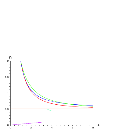
Figure 14: Curves in the $(\mu,n)$ phase diagram for the $(p,q)=(1,1)$, $(1,2){}_{\mathfrak{t}}$ and $(2,1)$ solutions in five dimensions. These curves lie in the region $1/2<n\leq 2$. The lowest (red) curve corresponds to the $(1,1)$ solution. The (blue) curve that has highest $n$ for high values of $\mu$ is the equal temperature $(1,2){}_{\mathfrak{t}}$ solution. The (green) curve that has highest $n$ for small values of $\mu$ is the $(2,1)$ solution. The entire phase space of the $(1,2)$ configuration is the wedge bounded by the equal temperature $(1,2){}_{\mathfrak{t}}$ curve and the $(1,1)$ curve. For completeness we have also included the uniform black string phase and sketched the non-uniform black string phase in the region $0\leq n\leq 1/2$. In this region we also plot the small black hole branch using the results of [22].

Inverting (8.5) we find

$$n_{(1,1)}(\mu)=\frac{1}{4}\left[-1+3\sqrt{1+\frac{8}{\mu^{2}}}\right]$$ (8.6)

We see that the lowest value for $\mu$ is obtained for the static bubble solution ($\mu=\mu_{\rm b}=1$ and $n=2$, see Table 1), while for large $\mu$ the value $n=1/2$ of the uniform black string in five dimensions is approached. We conclude that the branch of $(1,1)$ solutions consists of a curve in the $(\mu,n)$ phase diagram that starts in the point corresponding to the static bubble and approaches for infinite mass the horizontal line $n=1/2$ of the uniform black string. This will be the case for all curves that we explicitly obtain in this section.

To obtain the other thermodynamic variables of the solution we use (5.25) (and the formula below it) to compute the dimensionless entropy (defined in (2.6)) in terms of $x$. This result is then easily written as a function of $n$ using (8.4), yielding

$$\mathfrak{s}_{(1,1)}(n)=\frac{(2-n)^{3/2}}{(n+1)^{1/2}(2n-1)}\,.$$ (8.7)

From this we can find the temperature $\mathfrak{t}(n)$ for example, by using the Smarr formula (5.31) and the form of $\mu$ in (8.5). Alternatively, the temperature can be computed directly from (5.25), or one may use the first law of thermodynamics (2.8) to obtain $\mathfrak{t}(n)=\frac{\partial\mu}{\partial n}\left[\frac{\partial s}{\partial n}\right]^{-1}$. We also note that the curves $\mu_{(1,1)}(n)$ and $\mathfrak{s}_{(1,1)}(n)$ are correctly invariant under the map (7.6), (7.7) respectively.

The entropy $\mathfrak{s}$ as a function of $\mu$ can now be obtained by combining (8.7) with (8.5), yielding

$$\mathfrak{s}_{(1,1)}(\mu)=\frac{1}{2}\frac{\left(3-\sqrt{1+\frac{8}{\mu^{2}}}\right)^{3/2}}{\left(1+\sqrt{1+\frac{8}{\mu^{2}}}\right)^{1/2}\left(-1+\sqrt{1+\frac{8}{\mu^{2}}}\right)}\ .$$ (8.8)

We have plotted the resulting curve in Figure 15. We see from (8.8) that the entropy goes to zero, as expected, when the pure bubble configuration is approached at $\mu=1$. Moreover, we observe that leading term for large $\mu$ precisely corresponds to the (dimensionless) entropy of the uniform black string

$$\mathfrak{s}_{\rm bs}(\mu)=\frac{\mu^{2}}{4}\ ,\ \ d=4\,.$$ (8.9)

The latter result easily follows from the definitions (2.6) and the standard thermodynamics of the uniform black string in five dimensions. More genereally, the result in (8.8) explicitly shows

$$\mathfrak{s}_{(1,1)}(\mu)<\mathfrak{s}_{\rm bs}(\mu)\ ,\ \ \forall\;\,\mu\geq 1\,,$$ (8.10)

so that the $(1,1)$ configuration has lower entropy than that of the uniform black string. This property can also be argued from the Intersection Rule of Ref. [19] using the fact that in the $(\mu,n)$ phase diagram the $(1,1)$ solution approaches the uniform string from above for $\mu\rightarrow\infty$ (see Figure 14). As we will see in all our examples, this is a general feature of all the bubble-black hole sequences; some of the mass is spent in the bubbles, and hence the bubble-black hole sequences are going to have smaller horizon areas compared to the uniform black string of the same mass $\mu$.

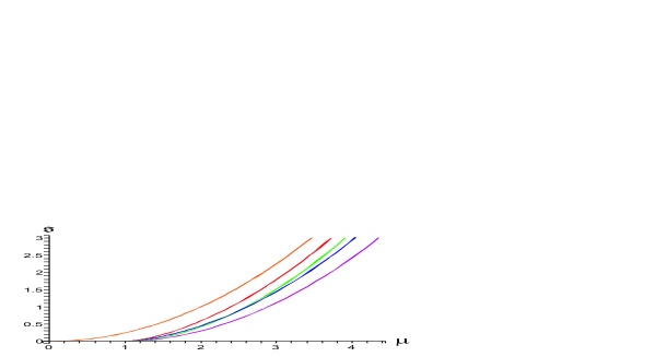
Figure 15: The dimensionless entropy $\mathfrak{s}$ as a function of the dimensionless mass $\mu$ for the $(0,1)$, $(1,1)$, $(2,1)$, $(1,2)_{\rm\mathfrak{t}}$ and $(2,3)_{\rm\mathfrak{t}}$ solutions in five dimensions. Here we have ordered the solutions as they appear from left to right in the figure for high mass (in terms of the colors used: orange, red, green, blue, purple). All $(p,q)$ curves approach for large $\mu$ the entropy curve of the $(0,1)$ solution, i.e. the uniform black string which has $\mathfrak{s}(\mu)=\mu^{2}/4$. The entropy curve of the $(2,1)$ solution (green) intersects the $(1,2)_{\rm\mathfrak{t}}$ solution (blue) in the point $\mu=\mu_{\star}\approx 2.42$. For comparison, the Gregory-Laflamme mass is $\mu_{\mathrm{GL}}\approx 3.52$.

Finally, for the mapping from the five-dimensional $(1,1)$ solution to the six-dimensional $(1,1)$ solution we need the length of the compact circle for the $(1,1)$ solution

$$L_{(1,1)}(n)=4\pi\sqrt{\frac{2n-1}{n+1}}\,,$$ (8.11)

as follows easily from (8.4).

$(1,1)$ configuration in $D=6$: black ring on bubble

The $(1,1)$ solution in six dimensions describes the configuration

$$\begin{array}[]{ccc}\mathrm{black~{}ring}&-&\mathrm{bubble}\\ S^{3}\times S^{1}&&D\times S^{1}\end{array}$$ (8.13)

consisting of an $S^{3}\times S^{1}$ black ring on a bubble of topology a disk times a circle. The exact form of the metric can be computed from (6.2), (6.3) with $N=3$. This solution was first obtained in Ref. [33].

The $S^{1}$ of the black ring does not wrap the Kaluza-Klein circle, but it is supported by the bubble. Without the bubble, a static black ring would collapse under its gravitational self-attraction, but just as a bubble can hold apart two black holes, we see that a bubble can also balance a black ring.

In order to obtain the thermodynamic results for the six-dimensional $(1,1)$ configuration, we use the map in (6.23), (6.24) and the curves (8.5), (8.7), (8.11) of the five-dimensional $(1,1)$ solution. Dropping the labels “6D”, the results are

$$\mu_{\mathrm{(1,1)}}(n)=\frac{4}{3n-1}\,,\hskip 28.45274pt\mathfrak{s}_{\mathrm{(1,1)}}(n)=\left(\frac{3-n}{3n-1}\right)^{3/2}\ ,\ \ 1/3<n<3\,,$$ (8.14)

and one can verify again that these are correctly invariant under (7.6), (7.7).

The $\mu_{\mathrm{(1,1)}}(n)$ curve is drawn in the $(\mu,n)$ phase diagram of Figure 16. In this case, the curve is easily inverted to give

$$n_{(1,1)}(\mu)=\frac{1}{3}+\frac{4}{3\mu}\,.$$ (8.15)

This shows that the lowest value of $\mu$ is obtained for the static bubble solution ($\mu=\mu_{\rm b}=1/2$ and $n=3$, see Table 1), while for large $\mu$ the value $n=1/3$ of the uniform black string is approached.

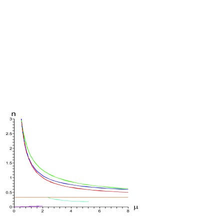
Figure 16: Curves in the $(\mu,n)$ phase diagram for the $(p,q)=(1,1)$, $(1,2)_{\mathfrak{t}}$ and $(2,1)$ solutions in six dimensions. These curves lie in the region $1/3<n\leq 3$. The lowest (red) curve corresponds to the $(1,1)$ solution. The (blue) curve that has highest $n$ for high values of $\mu$ is the equal temperature $(1,2)_{\mathfrak{t}}$ solution. The (green) curve that has highest $n$ for small values of $\mu$ is the $(2,1)$ solution. The entire phase space of the $(1,2)$ configuration is the wedge bounded by the equal temperature $(1,2)_{\mathfrak{t}}$ curve and the $(1,1)$ curve. For completeness we have also included the uniform and non-uniform black string phase (numerical data courtesy T. Wiseman), as well as the small black hole branch, lying in the region $0\leq n\leq 1/3$ (see Figure 2).

The two expressions in (8.14) can be combined to give the entropy function

$$\mathfrak{s}_{(1,1)}(\mu)=\bigg{[}\frac{2}{3}\Big{(}\mu-\frac{1}{2}\Big{)}\bigg{]}^{3/2}\,.$$ (8.16)

We see again that the entropy goes to zero as the pure bubble configuration is approached. Furthermore, the leading term for large $\mu$ corresponds to the (dimensionless) entropy of the uniform black string

$$\mathfrak{s}_{\rm bs}(\mu)=\left(\frac{2}{3}\,\mu\right)^{3/2}\ ,\ \ d=5$$ (8.17)

in six dimensions. Again it is not difficult to verify that the entropy of the entire $(1,1)$ branch is lower than that of the uniform black string for all $\mu\geq 1/2$.

8.2 Configurations with $(p,q)=(1,2)$ and $(2,1)$

The next two cases to be considered are the $(1,2)$ and $(2,1)$ configurations. As already discussed in Section 5, in five dimensions the $(1,2)$ solution describes two black holes held apart by a static bubble, and the $(2,1)$ solution is a black ring between two bubbles; we describe these five-dimensional configurations first. After that the corresponding six dimensional configurations are given.

$(1,2)$ configuration in $D=5$: Two black holes held apart by a bubble

The $(1,2)$ solution in five dimensions describes the configuration

$$\begin{array}[]{ccccc}\mathrm{black~{}hole}&-&\mathrm{bubble}&-&\mathrm{black~{}hole}\\ S^{3}&&S^{1}\times I&&S^{3}\end{array}$$ (8.18)

i.e. two $S^{3}$ black holes held apart by a bubble of cylinder topology $S^{1}\times I$. The metric is obtained by setting $N=4$ in (5.3), (5.4). This solution was studied in detail in [34].

As for the black hole in the $(1,1)$ solution, the black holes in the $(1,2)$ solution are not localized on the KK circle, and for a given size of the circle at infinity the black holes can be arbitrarily big. The sizes of the two black holes can be varied independently, and the bubble will vary its size and shape to balance the black holes and keep them in static equilibrium. In particular, one of the black holes can be removed, and the resulting configuration is an $S^{3}$ black hole on a bubble which is now topologically a disk $D$, i.e. the $(1,1)$ solution in (8.2).

To further analyze the solution quantitatively, we choose

$$(a_{1},a_{2},a_{3},a_{4})=(0,x,y,1)\ ,\ \ 0<x<y<1\,.$$ (8.19)

Using this in (5.28), we find from (5.30), (5.14) the dimensionless mass, relative tension and (rescaled) length of the compact circle

$$\mu=\frac{4\pi}{L}(2+x-y)\ ,\ \ n=\frac{1-x+y}{2+x-y}\ ,\ \ L=4\pi\frac{y-x}{\sqrt{y(1-x)}}\,.$$ (8.20)

We can substitute $L$ into $\mu$, and also use the expression for $n$ to eliminate $y$. This then determines the following family of curves in the $(\mu,n)$ phase diagram

$$\mu_{(1,2)}(n;\alpha)=\frac{3}{(n+1)(2n-1)}\sqrt{[n+1+(n-2)\alpha][2n-1+(2-n)\alpha]}$$ (8.21)

for

$$\frac{1}{2}<n<2\ ,\ \ 0\leq\alpha\leq 1\,,$$ (8.22)

where $\alpha$ parameterizes the branches in the family. Here, $\alpha=x/x_{\rm max}$, $x_{\mathrm{max}}\equiv\frac{2-n}{n+1}$ and the upper bound on $x$ comes from the condition $y<1$. The limits $\alpha=0$ and $\alpha=1$ correspond to removing either of the black holes, so we recover the $(1,1)$ configuration with one black hole on a bubble (see Section 8.1). These are in fact the solutions where for given $n$, the mass $\mu$ is minimized.

Another special case is where the two black holes have equal temperature. It is easily seen from (5.23) that this condition requires the two black holes to be of equal size. In order to arrange this we thus need to take the two black hole rods to have the same length ($a_{2}-a_{1}=a_{4}-a_{3}$) so that $y=1-x$ in the general expressions (8.20), and then $x$ runs in the range $0<x<1/2$. It is then not difficult to see that this corresponds to setting $\alpha=1/2$ in (8.21), from which it also follows that these are the solutions that maximize $\mu$ for fixed $n$. The resulting curve in the $(\mu,n)$ phase diagram is given by

$$\mu_{\mathrm{(1,2)_{\mathfrak{t}}}}(n)\equiv\mu_{\mathrm{(1,2)}}(n;\frac{1}{2})=\frac{9n}{2(n+1)(2n-1)}\ ,\ \ ~{}~{}\mbox{for}~{}~{}~{}\frac{1}{2}<n<2\,,$$ (8.23)

and is shown in Figure 14. We denote this branch as the $(1,2){}_{\mathfrak{t}}$ solution, where the $\mathfrak{t}$ subscript signifies the equal temperature property.

At this point some remarks are in order:
$\bullet$ Qualitatively, the parameter $\delta=|\alpha-1/2|$ can be regarded as a measure of the difference in size of the two black holes.
$\bullet$ To obtain physically distinct solutions it suffices to consider $0\leq\alpha\leq 1/2$ as the other half of the configurations are related by the $\mathbb{Z}_{2}$ symmetry $\alpha\rightarrow 1-\alpha$.
$\bullet$ The family of curves (8.21) fills a wedge in the phase diagram bounded by the $(1,1)$ curve (8.5) (minimal $\mu$ curve) and the equal temperature $(1,2)_{\mathfrak{t}}$ curve (8.23) (maximal $\mu$ curve), both of which are shown in Figure 14.
$\bullet$ As seen above in Section 8.2 for the $(1,1)$ curve, each branch labelled by $\alpha$ has $1\leq\mu\leq\infty$, and starts in the point corresponding to the static bubble and approaches for infinite mass the line $n=1/2$ of the uniform black string.

Similarly, we can compute the total dimensionless entropy $\mathfrak{s}=\frac{16\pi G_{N}}{L^{3}}(S_{1}+S_{2})$ using the entropy $S_{k}$ (given below (5.23)) for each black hole. This gives the total dimensionless entropy for the general $(1,2)$ solution as

$$\mathfrak{s}_{(1,2)}(n;\alpha)=\frac{(2-n)^{3/2}}{(n+1)(2n-1)^{2}}\left[\sqrt{\alpha^{3}[n+1+\alpha(n-2)]^{2}[2n-1+(2-n)\alpha]}\right.$$ (8.24)

$$+\left.\sqrt{(1-\alpha)^{3}[n+1+\alpha(n-2)][2n-1+(2-n)\alpha]^{2}}\right]$$

The temperatures $\mathfrak{t}_{1}$, $\mathfrak{t}_{2}$ of each of the black holes can be computed from (5.23).

For the special case of two equal-size black holes we obtain from (8.24)

$$\mathfrak{s}_{\mathrm{(1,2)_{\mathfrak{t}}}}(n)\equiv\mathfrak{s}_{(1,2)}(n;\frac{1}{2})=\frac{3\sqrt{3}}{4}\frac{n^{3/2}(2-n)^{3/2}}{(n+1)(2n-1)^{2}}\,.$$ (8.25)

In this case, since the temperatures are the same, one can use for example the Smarr formula (5.31) to obtain $\mathfrak{t}(n)$ from (8.23) and (8.25).

The expression (8.24) can be combined with (8.21), which determines a mass $\mu$ for given values of $(n;\alpha)$, to give the entropy as a function of mass. The entropy of all curves in the wedge satisfies the same property (8.10) as for the $(1,1)$ solution, and in particular for large $\mu$ the leading behavior is that of the uniform black string (8.9).

Within the family of solution branches parameterized by $\alpha$, one finds that for a given mass $\mu$, the configuration with highest entropy is the one with a single black hole on a bubble, while the configuration with lowest entropy is the one with two equal-size black holes. The latter fact is in accordance with the general result of Section 7.2 that solutions with equal temperatures extremize (in this case minimize) the entropy. The other configurations $0<\alpha<1/2$ interpolate between these two entropy extremes. This is illustrated in Figure 15, in which we plot $\mathfrak{s}$ versus $\mu$ for various configurations.

Finally, for use below we give the (rescaled) length of the compact circle for the $(1,2)$ solution

$$L_{(1,2)}(n;\alpha)=4\pi\frac{(2n-1)}{\sqrt{[n+1+(n-2)\alpha][2n-1+(2-n)\alpha]}}\ ,$$ (8.26)

which follows from (8.20).

$(2,1)$ configuration in $D=5$: Black ring between two equal size bubbles

The $(2,1)$ solution in five dimensions is described by the configuration

$$\begin{array}[]{ccccc}\mathrm{bubble}&-&\mathrm{black~{}ring}&-&\mathrm{bubble}\\ D&&S^{2}\times S^{1}&&D\end{array}$$ (8.29)

i.e. a black ring of topology $S^{2}\times S^{1}$ supported by two bubbles of disk topology. The exact form of the metric is obtained by setting $N=4$ in (5.5). This solution was studied in detail in [34].

The $S^{1}$ of the black ring is not the same $S^{1}$ as the KK circle at infinity. The black hole is therefore not topologically supported, which is the reason for calling it a black ring. The bubbles are topologically disks and they support the black ring from collapsing under its gravitational self-attraction. Note that this regular bubble-black ring solution is different from the asymptotically flat static black ring in [33] which was supported by a conically singular disk.

The physical parameters of this configuration can of course be obtained directly following similar steps as above, while taking into account the regularity constraint that the two bubbles should have equal size. It is easier, however, to obtain the physical parameters of the solution using the duality map of Section 7.1. This uses the fact that the $(2,1)$ solution can be obtained by a double Wick rotation $(t,\phi)\to(i\phi,it)$ from the configuration (8.18) with two equal-size black holes, i.e. the $(1,2){}_{\mathfrak{t}}$ solution.

Then, using the duality map (7.6), (7.7) we find from the mass and entropy curves (8.23), (8.25) of the $(1,2){}_{\mathfrak{t}}$ solution the dual curves

$$\mu_{(2,1)}(n)=\frac{3\sqrt{3}}{(n+1)\sqrt{2n-1}}\ ,\ \ \mathfrak{s}_{(2,1)}(n)=\frac{2(2-n)^{2}}{(n+1)(2n-1)}$$ (8.30)

of the $(2,1)$ solution. We have plotted the curve $\mu_{(2,1)}(n)$ in the $(\mu,n)$ phase diagram of Figure 14. Note that for small $\mu$ the black ring branch starts outside the wedge of solutions with two black holes on a bubble, but at a certain mass it cuts into the wedge and stays there. The intersection point in the $(\mu,n)$ phase diagram of the $(2,1)$ branch (8.30) with the $(1,2){}_{\mathfrak{t}}$ branch (8.35) (equal size black holes) is at $n=\frac{2}{3}$ and $\mu=\frac{27}{5}$. This is an explicit example of non-uniqueness in the $(\mu,n)$ phase diagram, as the two solutions are physically distinct. The corresponding curve for $\mathfrak{s}_{(2,1)}(\mu)$ is drawn in Figure 15, which asymptotes for large $\mu$ again to the expression in (8.9).

We can now also compare the entropies of the curves obtained so far. For small $\mu<\mu_{\star}\approx 2.42$ the $(2,1)$ solution (of a black ring between two bubbles) is the lowest entropy configuration. For $\mu>\mu_{\star}$, the $(2,1)$ solution has higher entropy than the $(1,2)_{\mathfrak{t}}$ solution (of two equal-size black holes on a bubble), but always lower entropy than the $(1,1)$ solution of a single black hole on the bubble. We observe (see Figure 15) that the uniform black string ($n=1/2$ for all $\mu$) has higher entropy than any of the bubble-black hole solutions, but we also note that for $\mu<\mu_{\mathrm{GL}}\approx 3.52$ the uniform black string is classically unstable. Based on the entropy consideration, the bubble-black hole sequences are globally unstable, however, this does not necessarily provide information about the local, or classical, stability of the configurations.

$(1,2)$ and $(2,1)$ configurations in $D=6$

The $(1,2)$ solution in six dimensions is described by the configuration

$$\begin{array}[]{ccccc}\mathrm{black~{}ring}&-&\mathrm{bubble}&-&\mathrm{black~{}ring}\\ S^{3}\times S^{1}&&T^{2}\times I&&S^{3}\times S^{1}\end{array}$$

consisting of two $S^{3}\times S^{1}$ black rings held apart by a bubble of topology cylinder times a circle. The bubble plays two roles for keeping the black rings in static equilibrium: it prevents each black ring from collapsing under its gravitational self-attraction (this is necessary since the rings are not topologically supported), and it also keeps the two black rings apart.

In order to obtain the physical parameters for the six-dimensional $(1,2)$ configuration we use again the mapping in (6.23), (6.24) and the five-dimensional results (8.21), (8.24), (8.26). After some algebra we find

$$\mu_{(1,2)}(n;\alpha)=\frac{2}{(n+1)(3n-1)^{2}}[2n+2+(n-3)\alpha][3n-1+(3-n)\alpha]\,,$$ (8.32)

$$\mathfrak{s}_{(1,2)}(n;\alpha) = \frac{(3-n)^{3/2}}{2(n+1)(3n-1)^{3}}\left[\sqrt{\alpha^{3}[2n+2+\alpha(n-3)]^{3}[3n-1+(3-n)\alpha]^{2}}\right.$$

$$\hskip 45.52458pt+\left.\sqrt{(1-\alpha)^{3}[2n+2+\alpha(n-3)]^{2}[3n-1+(3-n)\alpha]^{3}}\right]\ ,\ \$$

for

$$\frac{1}{3}<n<3\ ,\ \ 0\leq\alpha\leq 1\,.$$ (8.34)

The solution is qualitatively similar to the five-dimensional $(1,2)$ solution, and all remarks above apply here as well. In particular, we recover for $\alpha=0,1$ the $(1,1)$ solution of one black ring on a bubble given in Section 8.1. For $\alpha=1/2$ we find the configuration of two equal-size (and equal temperature) black rings on a bubble. The mass and entropy of this solution are

$$\mu_{(1,2)_{\mathfrak{t}}}(n)=\frac{(5n+1)^{2}}{2(n+1)(3n-1)^{2}}\ ,\ \ \mathfrak{s}_{(1,2)_{\mathfrak{t}}}(n)=\frac{(5n+1)^{5/2}(3-n)^{3/2}}{16(n+1)(3n-1)^{3}}\ .$$ (8.35)

The $\mu_{(1,2)_{\mathfrak{t}}}(n)$ curve is shown in Figure 16. From the two curves in (8.35) one may then obtain the entropy function $\mathfrak{s}_{(1,2)_{\mathfrak{t}}}(\mu)$. This has again the property that for large $\mu$ the entropy (8.17) of the uniform black string is approached.

Finally, we turn to the six dimensional $(2,1)$ configuration

$$\begin{array}[]{ccccc}\mathrm{bubble}&-&\mathrm{black~{}tuboid}&-&\mathrm{bubble}\\ D\times S^{1}&&S^{2}\times T^{2}&&D\times S^{1}\end{array}$$

consisting of a black tuboid of topology $S^{2}\times T^{2}$ supported by two equal size bubbles of topology $D\times S^{1}$. The $S^{1}$’s of the tuboid are prevented from collapse by the two equal size bubbles. In Section 6.3 we analyzed the horizon topology of the black tuboid. One interesting property is that the torus $T^{2}=S^{1}\times S^{1}$ of the horizon is non-trivially fibred over the $S^{2}$.

The physical parameters of this solution can be either obtained directly, or from the five dimensional $(2,1)$ solution using the map (6.23), (6.24), or from the six dimensional $(1,2){}_{\mathfrak{t}}$ solution above using the duality map of (7.6), (7.7). The results are

$$\mu_{(2,1)}(n)=\frac{2(n+5)}{(n+1)(3n-1)}\ ,\ \ s_{(2,1)}(n)=\frac{(n+5)^{1/2}(3-n)^{2}}{(n+1)(3n-1)^{3/2}}\,,$$ (8.37)

and the $\mu_{(2,1)}(n)$ curve is plotted in the phase diagram of Figure 16. Comparing to the five-dimensional phase diagram Figure 14, we see that the qualitative features are the same. Also in six dimensions, we see the feature that the $(2,1)$ branch of the tuboid intersects the $(1,2)_{\mathfrak{t}}$ branch of two equal-size black rings on bubble, this time in the point $n=7/13$ and $\mu=117/10$.

¿From the two curves in (8.37) one can obtain the entropy function $\mathfrak{s}_{(2,1)}(\mu)$, which again approaches the entropy (8.17) of the uniform black string for large $\mu$. In all, the $(\mu,\mathfrak{s})$ diagram is qualitatively the same as in five dimensions (see Figure 15). Again we find that among the bubble-black hole solutions, the entropically favored one is the $(1,1)$ solution with a single black ring on a bubble. The $(2,1)$ solution has higher entropy than the $(1,2){}_{\mathfrak{t}}$ solution for $\mu>\mu_{\star}\approx 2.61$. For comparison, $\mu_{\mathrm{GL}}\approx 2.31$. The six-dimensional uniform black string with entropy (8.17) is entropically favored over any of the bubble-black hole configurations that we have studied here.

8.3 Configurations with $(p,q)=(2,3)$, $(3,2)$ and $(2,2)$

Finally, we discuss some more involved, but still tractable, configurations, starting with the case $(p,q)=(2,3)$.

$(2,3)$ configuration in $D=5$

The $(2,3)$ solution in five dimensions is described by the configuration

$$\begin{array}[]{ccccccccc}\mathrm{black~{}hole}&-&\mathrm{bubble}&-&\mathrm{black~{}ring}&-&\mathrm{bubble}&-&\mathrm{black~{}hole}\\ S^{3}&&S^{1}\times I&&S^{2}\times S^{1}&&S^{1}\times I&&S^{3}\end{array}$$ (8.40)

In Figure 17 we sketch the geometry of the configuration. The general $(p,p+1)$ configuration has extra “$-\mathrm{bubble}-\mathrm{black~{}ring}-$” insertions. The explicit metric follows by setting $N=6$ in (5.3).

Figure 17: Sketch of the $(2,3)$ configuration of black holes and bubbles.

According to the discussion of Section 5.2, as soon as we have more than one bubble in the configuration, the regularity condition (5.15) imposes constraints on the parameters $a_{i}$ specifying the solution. In particular, for the $(2,3)$ solution the constraint is $L=(\Delta\phi)_{1}=(\Delta\phi)_{2}$. Using the general expressions (5.14) for $(\Delta\phi)_{k}$, this implies that

$$\frac{a_{3}-a_{2}}{a_{4}-a_{2}}\sqrt{\frac{a_{4}-a_{1}}{a_{3}-a_{1}}}=\frac{a_{5}-a_{4}}{a_{5}-a_{3}}\sqrt{\frac{a_{6}-a_{3}}{a_{6}-a_{4}}}\,.$$ (8.41)

Taken together with our conventions $a_{1}=0$, $a_{6}=1$, this means that there are three independent dimensionless parameters characterizing the general $(2,3)$ solution.

To simplify matters, we choose here to focus only on the subset of $(2,3)$ solutions for which the rod configurations have a $\mathbb{Z}_{2}$-symmetry of reflection in the line through its center. Such a configuration can generally be specified by choosing the $a_{i}$’s as follows

$$(a_{1},a_{2},a_{3},a_{4},a_{5},a_{6})=(0,x,x+y,1-2(x+y),1-(x+y),1-x,1)\ ,\ \$$ (8.42)

with two parameters $x,y$ such that

$$0<x<\frac{1}{2}-y\ ,\ \ 0<y<\frac{1}{2}\,.$$ (8.43)

This is a two-parameter solution of the constraint (8.41). Though we do not consider the entire phase space of the $(2,3)$ solution, this subset serves already as a useful illustration of the features of the solution. It is clear that the $\mathbb{Z}_{2}$ symmetry in (8.42) implies that the two black holes at the ends of the bubble-black hole sequence (8.40) are equal in size and that they have equal temperatures. Since we expect that the maximal $\mu$ curve in the $(\mu,n)$ phase diagram for the general $(2,3)$ solution corresponds to a configuration with this $\mathbb{Z}_{2}$ symmetry, this means that the subset under consideration here suffices to determine this curve.

As we have already provided details of the procedure of extracting the physical quantities for the simpler $(1,1)$, $(1,2)$ and $(2,1)$ solutions discussed above, we will be less extensive in the discussion below.

Using the rod structure (8.42) we find again $\mu$, $n$, and $L$ from (5.28), (5.30), and (5.14). The equation for $n$ can be solved for $y$ to give $y=(2n-1)/(2(n+1))$. Setting $x=x_{\rm max}\alpha$, $x_{\rm max}=1/2-y=(n-2)/(2(n+1))$, we obtain the following one-parameter family of curves

$$\mu_{(2,3)}(n;\alpha)=\frac{3}{2}\frac{[3+2\alpha(n-2)][2(n+1)+\alpha(n-2)]}{(n+1)(2n-1)[n+1+\alpha(n-2)]}\sqrt{\frac{2n-1-\alpha(n-2)}{3+\alpha(n-2)}}$$ (8.44)

for

$$\frac{1}{2}<n<2\ ,\ \ 0\leq\alpha\leq 1\,.$$ (8.45)

The curve for $\alpha=0$ reduces to the $(2,1)$ case (see (8.30) ) since the two $S^{3}$ black holes on the outside shrink to zero size. On the other hand, $\alpha=1$ reduces to the $(1,2){}_{\mathfrak{t}}$ case (see (8.23)) since the bubble in the middle is eliminated, and the black holes on the outside have equal temperature.

The family of curves (8.44) describes again a wedge of solutions in the $(\mu,n)$ phase diagram. The curves that form the bounds of the wedge are the maximal and minimal $\mu$ curves, found by extremizing the function $\mu_{(2,3)}$ as a function of $\alpha$. Details of this are given in Appendix A. The minimal $\mu$ curve for the symmetric solution is given in (A.2) and consists of a combination of the $(1,2){}_{\mathfrak{t}}$ and $(2,1)$ solution (see also Figure 14). However, the general $(2,3)$ configuration (without the symmetry) includes the $(1,1)$ solution, which we have seen gives the overall minimal $\mu$ curve. More interesting is therefore to consider the maximal $\mu$ curve of (8.44), as we expect this to be also the maximal $\mu$ curve of the general $(2,3)$ configuration. This curve is given in (A.3) and shown in Figure 18. It involves the solution $\alpha=\alpha_{\mu({\rm max})}(n)$ of a quartic equation on $\alpha$, with $n$-dependent coefficients in the range $0\leq\alpha\leq 1$.

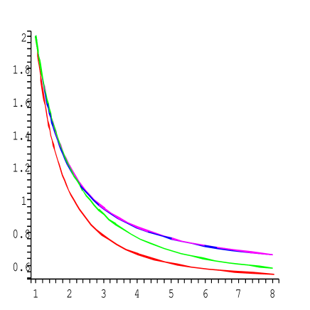
Figure 18: Curves in the $(\mu,n)$ phase diagram relevant for the $(p,q)=(2,3)$ solution in five dimensions. The highest (maximal $\mu$) curve (purple) is obtained in Appendix A. On this curve, the two black holes at the endpoint are at equal temperature, but the middle one has a lower temperature. The lowest (minimal $\mu$) curve (red) corresponds to the $(1,1)$ solution of Section 8.1. The $(2,3){}_{\mathfrak{t}}$ solution with all temperatures equal (and which also is the curve of minimal entropy) is the blue curve, which lies almost on top of the maximal $\mu$ curve. The green curve corresponds to the $(2,1)$ solution.

We also consider the total entropy of the one-parameter family,

$$\mathfrak{s}_{(2,3)}(n;\alpha)=\frac{(n-2)^{2}[2(n+1)+\alpha(n-2)][2n-1-\alpha(n-2)](1-\alpha)^{2}}{(n+1)(2n-1)^{2}[n+1+\alpha(n-2)]^{2}}$$ (8.46)

$$+\frac{(n-2)^{3/2}[3+2\alpha(n-2)]^{2}[2(n+1)+\alpha(n-2)]^{3/2}[2n-1-\alpha(n-2)]^{1/2}\alpha^{3/2}}{4(n+1)(2n-1)^{2}[n+1+\alpha(n-2)]^{2}[3+\alpha(n-2)]^{1/2}}$$

which can be combined with (8.21) to give the entropy function $\mathfrak{s}_{(2,3)}(\mu)$. It is interesting to find out what are the curves that minimize and maximize the entropy for a give $\mu$. The details of this computation can be found in Appendix A, and we present here the main results.

Within the family (8.21), the curve of maximum entropy is (just as the minimal $\mu$ curve) described by a combination (A.6) of the $(1,2){}_{\mathfrak{t}}$ and $(2,1)$ solutions (see also Figure 15). However, for the general $(2,3)$ solution, we expect that the overall maximal entropy curve will be given by the $(1,1)$ solution.

More interesting is to determine the minimal entropy curve. For the symmetric $(2,3)$ solution this curve follows by solving a quintic equation on $\alpha$ with $n$-dependent coefficients and we denote its solution as $\alpha=\alpha_{\mathfrak{s}(\rm min)}(n)$. The curve in the $(\mu,n)$ phase diagram is given by (A.8) and is shown in Figure 18, while the curve in the $(\mu,\mathfrak{s})$ diagram is given in (A.7) and plotted in Figure 15.

We can now explicitly check the general result of Section 7.2 that the equal temperature case should correspond to an extremum of the entropy. As remarked above, for any $\alpha$ we have that $\mathfrak{t}_{1}=\mathfrak{t}_{3}$ (because the solution is symmetric) but not necessarily equal to $\mathfrak{t}_{2}$. Equating also $\mathfrak{t}_{1}=\mathfrak{t}_{2}$, we find from (5.23) a quintic equation on $\alpha$, whose solutions we denote by $\alpha=\alpha_{\mathfrak{t}}(n)$. We then find, in accordance with Section 7.2 that

$$\alpha_{\mathfrak{t}}(n)=\alpha_{\mathfrak{s}(\rm min)}(n)$$ (8.47)

i.e. the curve minimizing the total entropy coincides with the curve describing the special case where all temperatures of the three black holes in the $(2,3)$ solution are equal. We denote this configuration therefore as the $(2,3){}_{\mathfrak{t}}$ solution. The corresponding curve (coinciding with the minimum entropy case) is shown in Figures 18 and 15.

Finally, we comment on the issue of non-uniqueness in the $(\mu,n)$ phase diagram. First, we note that the $(2,3){}_{\mathfrak{t}}$ solution intersects the $(2,1)$ solution in the point $(\mu,n)\approx(2.149,1.139)$. Just as the earlier observed intersection point of the $(1,2){}_{\mathfrak{t}}$ and $(2,1)$ solution, this is another explicit example of non-uniqueness.

More generally, we can argue for infinite non-uniqueness in the $(2,3)$ solution as follows. We have seen that the two-parameter family of $\mathbb{Z}_{2}$ symmetric $(2,3)$ solutions describe a two-dimensional wedge in the phase diagram bounded from above by the maximal $\mu$ curve of the $(2,3)$ solution and from below by a combination of the $(1,2){}_{\mathfrak{t}}$ solution and the $(2,1)$ solution. More generally, we argued that the full $(2,3)$ solution should cover the wedge bounded from above by this maximal $\mu$ curve and from below by the $(1,1)$ solution. If one now imagines relaxing the $\mathbb{Z}_{2}$ condition, we know that: i) A larger region of the phase diagram starts to be covered as we are now able to go all the way down to the $(1,1)$ curve. ii) Since the $(2,3)$ solution has $q=3$ free parameters we can write $n=n(\mu,\alpha,\beta)$ where $\beta$ parameterizes the asymmetry. Since we have one more additional parameter that we can vary this implies that in the entire two-dimensional wedge accessible to the $(2,3)$ solution there is a subregion for which there should be infinite non-uniqueness specified by the extra parameter.

$(3,2)$ configuration in $D=5$

The $(3,2)$ solution in five dimensions is described by the configuration

$$\begin{array}[]{ccccccccc}\mathrm{bubble}&-&\mathrm{black~{}ring}&-&\mathrm{bubble}&-&\mathrm{black~{}ring}&-&\mathrm{bubble}\\ D&&S^{2}\times S^{1}&&S^{1}\times I&&S^{2}\times S^{1}&&D\end{array}$$ (8.50)

We restrict our quantitative analysis to the case where the two black holes have equal temperatures. We call this the $(3,2){}_{\mathfrak{t}}$ solution.

¿From Section 7.1 we know that this case can be obtained by Wick rotation from the equal temperature $(2,3){}_{\mathfrak{t}}$ solution, which we just discussed. Substituting the solution $\alpha=\alpha_{\mathfrak{t}}(n)$ in the curves (8.44), (8.46) and subsequently using the mapping (7.6), (7.7) it is relatively easy to find the corresponding curve for the $(3,2){}_{\mathfrak{t}}$ solution in the $(\mu,n)$ phase diagram. It starts for low $\mu$ above the wedge containing the $(2,3)$ solution, but then for some value of $\mu$ cuts into it and stays within the wedge. This feature is thus similar as that seen before for the $(2,1)$ solution, which cuts into the wedge containing the $(1,2)$ solutions (cf. Figure 14).

$(2,2)$ configuration in $D=5$

The $(2,2)$ solution in five dimensions is described by the configuration

$$\begin{array}[]{ccccccc}\mathrm{black~{}hole}&-&\mathrm{bubble}&-&\mathrm{black~{}ring}&-&\mathrm{bubble}\\ S^{3}&&S^{1}\times I&&S^{2}\times S^{1}&&D\end{array}$$ (8.53)

Note that this is the simplest solution that has objects of all possible topologies encountered in the five dimensional case in it. However, due to the lack of symmetry, this case is more difficult to treat in practice than the cases considered above, even though there are only two independent dimensionless quantities specifying the configuration.

$(2,3)$, $(3,2)$ and $(2,2)$ configurations in $D=6$

The preceding analysis in five dimensions can easily be repeated for six dimensions, and the topology of the objects will change accordingly. Moreover, the results above can be used to find the corresponding six dimensional ones using the map in (6.23), (6.24). In particular, we can use these transformations directly on the curves of Figures 18, 15, and it is found that all qualitative features are the same as in five dimensions.

9 Conclusions

We conclude the paper with the following general remarks and open problems:

Phase diagram: We have seen in this paper that the five- and six-dimensional bubble-black hole sequences that we constructed fall into the upper region, $1/(d-2)<n\leq d-2$ of the $(\mu,n)$ phase diagram of static Kaluza-Klein black holes. We also have the lower bound $\mu\geq\mu_{\rm b}$ for the (dimensionless) mass of each sequence, where $\mu_{\rm b}$ is the mass of the static Kaluza-Klein bubble.

Based on the general construction as well as the examples, it appears that the set of all bubble-black hole sequences covers a very large part of this region of the phase diagram and that there is a high degree of non-uniqueness. In particular, we note the following features:

• Among all the examples, the $(1,1)$ solution gives the curve in the $(\mu,n)$ phase diagram that has the lowest mass for given relative tension $n$. In other words for all other examples the curves lie above the curve of the $(1,1)$ solution. We believe this to hold in general for all bubble-black hole sequences.

• As we increase the number of bubbles and/or black holes in the sequence the curves of maximal mass (for given $n$) move upward. Physically this means that as we increase the number of objects in the sequence, one can achieve a higher relative tension for a given mass. It would be interesting to examine whether the entire area of the phase diagram above the $(1,1)$ solution is filled up all the way to (but not including) the horizontal line $n=d-2$.

• For a given $(p,q)$ solution with $p$ bubbles and $q$ black holes there are $q$ free parameters, corresponding to the relative sizes of the black holes. At the level of the phase diagram this implies the following important facts. For $q=1$ the solution is a curve in the phase diagram and for $q=2$ the solution is a two-dimensional wedge in the phase diagram. For $q\geq 3$ we continue to have two-dimensional wedges in the phase diagram, but there must be infinite non-uniqueness since there are still $q-2$ further parameters characterizing the solution.

  To see this more clearly, note that we can write $n=n(\mu,x_{1},\ldots,x_{q-1})$, since we can choose $\mu$ as one of the $q$ parameters of the $(p,q)$ solution. If $q=1$ we find a one-dimensional curve in the $(\mu,n)$ phase diagram. If $q=2$ there is one additional parameter so that we find a two-dimensional wedge in the $(\mu,n)$ phase diagram. For higher $q$ we have in addition $q-2$ parameters that can vary independently for given $\mu$ and $n$. We thus conclude that for a given $(p,q)$ solution with $q\geq 3$ there is an infinite non-uniqueness in the accessible region.

• The non-uniqueness becomes even more plentiful once we consider the entire set of bubble-black hole sequences in the phase diagram. To see this note that any $(p,p)$ or $(p,p+1)$ solution includes as a special case the $(1,1)$ solution. In other words the parameters specifying these solutions can be chosen arbitrarily close to the $(1,1)$ solution. So as we increase the number of objects in the sequence we have two effects. On the one hand, we find more solutions in the (“low”) region where we already had solutions. On the other hand, we find that we start to cover a “higher” region that was not covered before. It would be interesting to examine this further and prove these assertions mathematically rigorous.

• We also recall here that we have observed explicit cases of non-uniqueness in the intersection points of the $(1,2){}_{\mathfrak{t}}$ solution and the $(2,1)$ solution, as well as the intersection of $(2,3){}_{\mathfrak{t}}$ and the $(2,1)$ solution.

It is also possible to arrive at general statements regarding the entropy as a function of the mass.

• In the examples, the curve with highest entropy for a given mass $\mu$, is the one obtained for the $(1,1)$ solution. We believe that this curve represents the upper bound for the entropy curves of all $(p,q)$ solutions. Moreover, as the number of objects in the sequence increases, the corresponding entropy curves will tend to lie lower, but there can be non-trivial intersections.

• We have proven that, within a family of $(p,q)$ solutions the curve for the equal temperature $(p,q)_{\mathfrak{t}}$ solution corresponds to an extremum of the entropy, and we have observed in the examples that this is always the minimum entropy curve. This feature can be physically understood by considering two widely separated Schwarzschild black holes. For fixed total mass, the entropy of this configuration is minimized when the black holes have the same radius (hence same temperature), while the maximal entropy configuration is the one where all the mass is located in a single black hole.

• From the examples it appears that for any branch of $(p,q)$ solutions the entropy function approaches that of the uniform black string $\propto\mu^{\frac{d-2}{d-3}}$ in the limit of large mass, and the uniform black string has higher entropy than any of the $(p,q)$ solutions. The physical reason to expect that all bubble-black hole sequences have lower entropy than a uniform string of same mass, is that some of the mass has gone into the bubble rather than the black holes, giving a smaller horizon area for the same mass.

Topology: The bubble-black hole sequences that we have constructed involve event horizons of various topologies. In particular, in five dimensions we have $S^{3}$ (black hole) and $S^{2}\times S^{1}$ (black ring) topology. Moreover, in six dimensions we observed $S^{3}\times S^{1}$ (black ring) and $S^{2}\times S^{1}\times S^{1}$ (black tuboid) topology. In all cases, the $S^{1}$’s are not in the Kaluza-Klein direction (and hence not topologically supported), but supported by the Kaluza-Klein bubbles. It is interesting to note that the six-dimensional sequences we constructed do not involve event horizons with black hole topology $S^{4}$. It is not difficult to see that such sequences, if they exist, would not have four but only three commuting Killing isometries, and are hence not contained in the generalized Weyl ansatz used here. It would be interesting to examine whether more general classes of bubble-black hole sequences exist, in less symmetric ansätze, that would include the topology $S^{4}$.

General $D$: We have found a map between five- and six-dimensional bubble-black hole solutions. The general structure of the solutions was very similar in five and six dimensions, but the topologies of bubbles and black holes changed. It is interesting to ask if solutions for bubble-black hole sequences exist for $D\geq 7$, and if so, whether they can be related to the solutions of this paper by a map similar to the one mapping five- to six-dimensional solutions. Along these lines also follows the question about the $1/(d-2)<n\leq d-2$ region of the phase diagram. For $D\geq 7$, there are (apart from the static bubble at $(\mu_{\rm b},d-2)$) no known solutions in this region. It is tempting to speculate that for $D\geq 7$ this region is occupied by bubble-black hole sequences with features similar to the ones found in this paper for the five- and six-dimensional cases. It would be interesting if one could find bubble-black hole sequences in $\mathcal{M}^{d}\times S^{1}$ for $D=d+1\geq 7$. However, this may be difficult since one cannot use the generalized Weyl ansatz for such solutions.

On the other hand, one can easily construct rod configurations for Weyl solutions describing regular bubble-black hole sequences in dimensions greater than six. However, these solutions will have more than one Kaluza-Klein circle, i.e. asymptotics $\mathcal{M}^{d}\times T^{k}$, and the bubbles will be associated with different Kaluza-Klein directions. One potentially interesting example arises from the rod configuration depicted in Figure 19.

Figure 19: Rod configuration for black tuboid with two bubbles in seven dimensions.

This configuration describes a seven-dimensional black tuboid with horizon topology $S^{3}\times S^{1}\times S^{1}$ supported by two bubbles of topology $D\times S^{1}\times S^{1}$. Asymptotically the solution is $\mathcal{M}^{5}\times T^{2}$. It could be interesting to study the phase diagram for that class of solutions.

Stability: We have found that the entropy of the $(1,1)$ solution is less than that of the uniform black string with the same mass $\mu$. Also the examples showed that the $(p,q)$ solutions with more bubbles and black holes all had entropy lower than the $(1,1)$ solution. This indicates that the $(p,q)$ solutions are globally unstable. It is interesting to ask if the bubble-black hole sequences are also classically unstable.

The bubbles hold the black holes in a fine-tuned equilibrium. For the $(1,2)$ solution with two small black holes on a bubble, one can imagine perturbing the position of one black hole, causing it to ”slide” around the bubble to merge with the other black hole. This could be viewed as a decay of the $(1,2)$ solution to (a perturbed version of) the $(1,1)$ solution.

As discussed in Section 3, the static Kaluza-Klein bubble is classically unstable to perturbations that make it collapse or expand. There are $(p,q)$ solutions arbitrarily close to the pure bubble solutions, so we may expect these solutions to be clasically unstable too.

Another classical instability mode is that of the black rings supported by the bubbles. One can choose the parameters such that the black ring is long and thin, in which case a Gregory-Laflamme type instability mode could appear. It would be interesting to examine if the bubbles help stabilizing the black ring, or cause it to be even more unstable.

Periodic array: Imagine extending a rod configuration to include infinitely many finite rods arranged periodically. This effectively describes the covering space of a rod configuration with a compact $z$-direction. In five and six dimensions the asymptotic space-time has (at least) two circles, one parameterized by $\phi$ and the other by $z$. Potentially this makes the six-dimensional solution more interesting since it has four uncompactified dimensions. The solutions describe periodic arrays of black holes and bubbles. This is an uncharged analogue of arrays of supersymmetric black holes, but for the neutral bubble-black hole arrays we expect the bubbles to play a role in balancing the configurations. Generalizing the phase diagram to include configurations with non-trivial tensions in two compact directions, it could be interesting to study the phases of black hole arrays in Kaluza-Klein theory.

More solutions: Finally, we note that one can argue for the existence of new classes of solutions similar to the bubble-black hole sequences presented in this paper. Imagine taking the five-dimensional $(1,1)$ solution and throwing some matter into the black hole in such a way that the solution acquires an angular momentum. This suggest the existence of new $(1,1)$ solutions with angular momentum. However, since these solutions are stationary rather than static they are not part of the class of solutions studied in this paper. But, if we make a double Wick rotation in the $t$ and $\phi$-direction, as in Section 7.1, it seems likely that we get a static solution with one black hole and one Kaluza-Klein bubble that asymptote $\mathcal{M}^{4}\times S^{1}$. Therefore, the existence of the rotating $(1,1)$ solution imply the existence of a whole new continuous class of static solutions that should be part of the $(\mu,n)$ phase diagram.

Another way to argue for this is to take the four-dimensional Kerr solution [46], adding a trivial $\phi$-direction, and making a double Wick rotation in the $t$ and $\phi$-direction. This gives a continuous class of static Kaluza-Klein bubble solutions [47] which clearly all have $n=d-2$. This class of bubble solutions precisely correspond to the $n\rightarrow d-2$ limit of the new continuous class of static solutions with one bubble and one black hole that we argued above should exists. Similarly, one could argue for new classes of solutions in six dimensions.

Bubble-black hole sequences with charge: Using the methods of [50], one can put charge on the bubble-black hole sequences considered in this paper. This we explore in [51].

Appendix A Details on the $(p,q)=(2,3)$ solution

Given the family of curves $\mu_{(2,3)}(n;\alpha)$ (see (8.44)) of the $\mathbb{Z}_{2}$ symmetric $(2,3)$ configuration, we give here some details on the various special curves discussed in Section 8.3.

Extremal mass curves

To find the curves that extremize the mass in the range $\frac{1}{2}<n<2$, we set $\partial\mu_{(2,3)}(n;\alpha)/\partial\alpha=0$ which results in the following fourth order equation on the parameter $\alpha$

$$2(n-2)^{4}\alpha^{4}+2(n+7)(n-2)^{3}\alpha^{3}+2(n+4)^{2}(n-2)^{2}\alpha^{2}$$ (A.1)

$$-(n+1)(4n^{2}-7n-29)(n-2)\alpha-9(n+1)(2n^{2}-2n-1)=0$$

but at the same time we should remember that $0\leq\alpha\leq 1$, so that the extrema can also occur on the boundaries of the parameter space. Some analysis then shows that the minimal $\mu$ curve always lies on the boundary of parameter space

$$\mu_{(2,3)}^{\rm max}(n)=\left\{\begin{array}[]{cc}\mu_{(2,3)}(n;0)=\mu_{(1,2)_{\mathfrak{t}}}(n)&\ ,\ \ 1\leq\mu\leq\frac{27}{5}\\ \mu_{(2,3)}(n;1)=\mu_{(2,1)}(n)&\ ,\ \ \mu\geq\frac{27}{5}\end{array}\right.$$ (A.2)

where we recall that the $(1,2)_{\mathfrak{t}}$ and $(2,1)$ curves are given in (8.21), (8.30) respectively. This result should also be clear from Figure 14.

On the other hand, the corresponding value $\alpha_{\mu({\rm max})}(n)$ that maximizes $\mu$ is more complicated and is plotted as a function of $n$ in Figure 20. The behavior is slightly non-trivial. For $n\geq\frac{1}{2}(1+\sqrt{3})\simeq 1.336$ the maximum value occurs for $\alpha=0$, i.e. the $(1,2)_{\mathfrak{t}}$ solution. For $n<\frac{1}{2}(1+\sqrt{3})$ we find a non-trivial solution for $\alpha$ by solving (A.1). This has the property that for $n\rightarrow\frac{1}{2}$ we approach $\alpha=1$, i.e. the $(2,1)$ solution.

In conclusion, the curve that maximizes $\mu$ for a given $n$ is given by

$$\mu_{(2,3)}^{\rm max}(n)=\mu_{(2,3)}(n;\alpha_{\mu({\rm max})}(n))$$ (A.3)

where $\mu_{(2,3)}(n,\alpha)$ is given in (8.44) and $\alpha_{\mu({\rm max})}(n)$ the numerically obtained result in Figure 20.

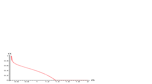
Figure 20: The solution $\alpha_{\mu({\rm max})}(n)$ that determines the maximum $\mu$ curve for the symmetric $(2,3)$ solution.

Using (5.23), we have also computed the temperatures $\mathfrak{t}_{1}=\mathfrak{t_{3}}$ and $\mathfrak{t}_{2}$ of the black holes for the symmetric $(2,3)$ solution with maximal mass. The result is plotted in Figure 21. This shows that the temperature of the black holes at the two ends of the sequence is higher than that of the black hole in the middle. We also see, for each of these, that as the black hole becomes smaller its temperature approaches infinity. For the black holes at the ends this happens at $n=\frac{1}{2}(1+\sqrt{3})$, after which the black holes have disappeared. For the black hole in the middle the temperature diverges at $n=2$, when only the bubble is left. We note, however, that the product $\mathfrak{t}\mathfrak{s}$ in this point is correctly zero, as required by the Smarr formula (5.31).

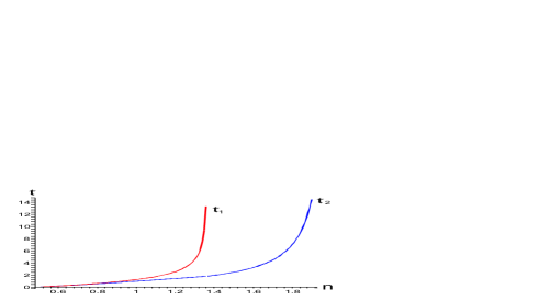
Figure 21: The temperatures $\mathfrak{t}_{1}=\mathfrak{t_{3}}$ and $\mathfrak{t}_{2}$ of the black holes for the maximal mass symmetric $(2,3)$ solution.

Extremal entropy curves

To find the curves that extremize the total entropy $\mathfrak{s}(\mu)$ (which is obtained from (8.44) and (8.46)), we proceed as follows.

After some standard variational calculus, the condition for an extremum of the entropy at fixed $\mu$ is

$$\frac{\partial s(n;\alpha)}{\partial n}\frac{\partial\mu(n;\alpha)}{\partial\alpha}=\frac{\partial s(n;\alpha)}{\partial\alpha}\frac{\partial\mu(n;\alpha)}{\partial n}$$ (A.4)

in the continuous region $0\leq\alpha\leq 1$, but we should again remember that extrema can occur on the boundaries of our parameter space. After some algebra the condition (A.4) gives rise to the quintic equation on the parameter $\alpha$

$$-32(2-n)^{4}\alpha^{5}+8(2-n)^{3}(2n+29)\alpha^{4}+8(2-n)^{2}(4n^{2}-16n-83)\alpha^{3}$$ (A.5)

$$-(2-n)(8n^{3}+180n^{2}-366n-943)\alpha^{2}-2(n+1)(8n^{3}-36n^{2}-114n+335)\alpha+48(n+1)^{2}(2-n)=0$$

where we have used also that we are only interested in solutions for which $0\leq\alpha\leq 1$.

We then find that the curve of maximum entropy lies on the boundary of parameter space and is given by

$$\mathfrak{s}_{(2,3)}^{\rm max}(\mu)=\left\{\begin{array}[]{cc}\mathfrak{s}_{(2,3)}(\mu)|_{\alpha=0}=\mathfrak{s}_{(1,2)_{\mathfrak{t}}}(\mu)&\ ,\ \ \mu\leq 2.42\\ \mathfrak{s}_{(2,3)}(\mu)|_{\alpha=1}=\mathfrak{s}_{(2,1)}(\mu)&\ ,\ \ \mu\geq 2.42\end{array}\right.$$ (A.6)

i.e. a particular combination of the $(1,2){}_{\mathfrak{t}}$ and $(2,1)$ solutions (just as the minimal $\mu$ curve (A.2)). Again this should also be clear from Figure 15. The corresponding crossover point in the $(\mu,n)$ diagram has $n=0.95$ on the $(1,2){}_{\mathfrak{t}}$ curve and $n=1.05$ on the $(2,1)$ curve, so there is a discontinuity in $n$.

On the other hand, for the minimum of the entropy, we find that $\alpha$ is given by the unique non-trivial solution $\alpha_{\mathfrak{s}({\rm min})}(n)$ of the quintic equation (A.5) in the range $0\leq\alpha\leq 1$. The numerically obtained solution is shown in Figure 22. We conclude that the minimum entropy curve is given by

$$\mathfrak{s}_{(2,3)}^{\rm min}(\mu)=\mathfrak{s}_{(2,3)}(n;\alpha_{\mathfrak{s}({\rm min})})|_{n=n_{\star}(\mu)}$$ (A.7)

where $n_{\star}(\mu)$ is found by inverting the curve

$$\mu_{(2,3)}^{\mathfrak{s}({\rm min})}(n)\equiv\mu_{(2,3)}(n;\alpha_{\mathfrak{s}({\rm min})}(n))$$ (A.8)

where $\mathfrak{s}_{(2,3)}(\mu;\alpha)$ and $\mu_{(2,3)}(\mu,\alpha)$ are given in (8.46), (8.44) respectively, and $\alpha_{\mathfrak{s}({\rm min})}(n)$ the numerically obtained result in Figure 22.

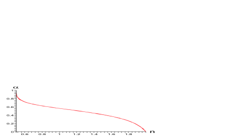
Figure 22: The solution $\alpha_{\mathfrak{s}({\rm min})}(n)$ that determines the minimum entropy curve for the symmetric $(2,3)$ solution. This coincides with the solution $\alpha_{\mathfrak{t}}(n)$ that determines the equal temperature $(2,3)$ solution.

Equal temperature curve

To find the equal temperature curve we use the temperature expressions in (5.23) along with the rod structure (8.42). Requiring $\mathfrak{t}_{1}=\mathfrak{t}_{2}$ and using the definitions above (8.44), one finds that this condition becomes a quintic equation on $\alpha$ with $n$-dependent coefficients. The solution of this equation in the range $0\leq\alpha\leq 1$ which we denote by $\alpha_{\mathfrak{t}}(n)$ is then seen to exactly agree with that of $\alpha_{\mathfrak{s}({\rm min})}(n)$ plotted in Figure 22. This explicitly shows that equal temperature corresponds to an extremum (here a minimum) of the total entropy.

References

- [1] W. Israel, “Event horizons in static vacuum space-times,” Phys. Rev. 164 (1967) 1776–1779.
- [2] B. Carter, “Axisymmetric black hole has only two degrees of freedom,” Phys. Rev. Lett. 26 (1971) 331–333.
- [3] S. W. Hawking, “Black holes in General Relativity,” Commun. Math. Phys. 25 (1972) 152–166.
- [4] D. C. Robinson, “Uniqueness of the Kerr black hole,” Phys. Rev. Lett. 34 (1975) 905–906.
- [5] G. W. Gibbons, D. Ida, and T. Shiromizu, “Uniqueness and non-uniqueness of static vacuum black holes in higher dimensions,” Prog. Theor. Phys. Suppl. 148 (2003) 284–290, gr-qc/0203004.
- [6] G. W. Gibbons, D. Ida, and T. Shiromizu, “Uniqueness and non-uniqueness of static black holes in higher dimensions,” Phys. Rev. Lett. 89 (2002) 041101, hep-th/0206049.
- [7] F. R. Tangherlini, “Schwarzschild field in n dimensions and the dimensionality of space problem,” Nuovo Cimento 27 (1963) 636.
- [8] R. C. Myers and M. J. Perry, “Black holes in higher dimensional space-times,” Ann. Phys. 172 (1986) 304.
- [9] R. Emparan and H. S. Reall, “A rotating black ring in five dimensions,” Phys. Rev. Lett. 88 (2002) 101101, hep-th/0110260.
- [10] S. S. Gubser, “On non-uniform black branes,” Class. Quant. Grav. 19 (2002) 4825–4844, hep-th/0110193.
- [11] T. Wiseman, “Static axisymmetric vacuum solutions and non-uniform black strings,” Class. Quant. Grav. 20 (2003) 1137–1176, hep-th/0209051.
- [12] T. Wiseman, “From black strings to black holes,” Class. Quant. Grav. 20 (2003) 1177–1186, hep-th/0211028.
- [13] M. W. Choptuik et al., “Towards the final fate of an unstable black string,” Phys. Rev. D68 (2003) 044001, gr-qc/0304085.
- [14] E. Sorkin, B. Kol, and T. Piran, “Caged black holes: Black holes in compactified spacetimes. II: 5d numerical implementation,” Phys. Rev. D69 (2004) 064032, hep-th/0310096.
- [15] H. Kudoh and T. Wiseman, “Properties of Kaluza-Klein black holes,” Prog. Theor. Phys. 111 (2004) 475–507, hep-th/0310104.
- [16] E. Sorkin, “A critical dimension in the black-string phase transition,” Phys. Rev. Lett. 93 (2004) 031601, hep-th/0402216.
- [17] T. Harmark and N. A. Obers, “Black holes on cylinders,” JHEP 05 (2002) 032, hep-th/0204047.
- [18] T. Harmark and N. A. Obers, “Black holes and black strings on cylinders,” Fortsch. Phys. 51 (2003) 793–798, hep-th/0301020.
- [19] T. Harmark and N. A. Obers, “New phase diagram for black holes and strings on cylinders,” Class. Quantum Grav. 21 (2004) 1709–1724, hep-th/0309116.
- [20] B. Kol, E. Sorkin, and T. Piran, “Caged black holes: Black holes in compactified spacetimes. I: Theory,” Phys. Rev. D69 (2004) 064031, hep-th/0309190.
- [21] T. Harmark and N. A. Obers, “Phase structure of black holes and strings on cylinders,” Nucl. Phys. B684 (2004) 183–208, hep-th/0309230.
- [22] T. Harmark, “Small black holes on cylinders,” Phys. Rev. D69 (2004) 104015, hep-th/0310259.
- [23] D. Gorbonos and B. Kol, “A dialogue of multipoles: Matched asymptotic expansion for caged black holes,” JHEP 06 (2004) 053, hep-th/0406002.
- [24] R. Gregory and R. Laflamme, “Black strings and p-branes are unstable,” Phys. Rev. Lett. 70 (1993) 2837–2840, hep-th/9301052.
- [25] T. Harmark and N. A. Obers, “General definition of gravitational tension,” JHEP 05 (2004) 043, hep-th/0403103.
- [26] G. T. Horowitz and K. Maeda, “Fate of the black string instability,” Phys. Rev. Lett. 87 (2001) 131301, hep-th/0105111.
- [27] R. Gregory and R. Laflamme, “Hypercylindrical black holes,” Phys. Rev. D37 (1988) 305.
- [28] G. T. Horowitz, “Playing with black strings,” hep-th/0205069.
- [29] B. Kol, “Topology change in general relativity and the black-hole black-string transition,” hep-th/0206220.
- [30] B. Kol and T. Wiseman, “Evidence that highly non-uniform black strings have a conical waist,” Class. Quant. Grav. 20 (2003) 3493–3504, hep-th/0304070.
- [31] R. Emparan, “Rotating circular strings, and infinite non-uniqueness of black rings,” JHEP 03 (2004) 064, hep-th/0402149.
- [32] E. Witten, “Instability of the Kaluza-Klein vacuum,” Nucl. Phys. B195 (1982) 481.
- [33] R. Emparan and H. S. Reall, “Generalized Weyl solutions,” Phys. Rev. D65 (2002) 084025, hep-th/0110258.
- [34] H. Elvang and G. T. Horowitz, “When black holes meet Kaluza-Klein bubbles,” Phys. Rev. D67 (2003) 044015, hep-th/0210303.
- [35] J. H. Traschen, “A positivity theorem for gravitational tension in brane spacetimes,” Class. Quant. Grav. 21 (2004) 1343–1350, hep-th/0308173.
- [36] T. Shiromizu, D. Ida, and S. Tomizawa, “Kinematical bound in asymptotically translationally invariant spacetimes,” Phys. Rev. D69 (2004) 027503, gr-qc/0309061.
- [37] H. S. Tan and E. Teo, “Multi-black hole solutions in five dimensions,” Phys. Rev. D68 (2003) 044021, hep-th/0306044.
- [38] J. H. Traschen and D. Fox, “Tension perturbations of black brane spacetimes,” Class. Quant. Grav. 21 (2004) 289–306, gr-qc/0103106.
- [39] P. K. Townsend and M. Zamaklar, “The first law of black brane mechanics,” Class. Quant. Grav. 18 (2001) 5269–5286, hep-th/0107228.
- [40] R. Gregory and R. Laflamme, “The instability of charged black strings and p-branes,” Nucl. Phys. B428 (1994) 399–434, hep-th/9404071.
- [41] D. J. Gross, M. J. Perry, and L. G. Yaffe, “Instability of flat space at finite temperature,” Phys. Rev. D25 (1982) 330–355.
- [42] D. Brill and G. T. Horowitz, “Negative energy in string theory,” Phys. Lett. B262 (1991) 437–443.
- [43] S. Corley and T. Jacobson, “Collapse of Kaluza-Klein bubbles,” Phys. Rev. D49 (1994) 6261–6263, gr-qc/9403017.
- [44] O. Sarbach and L. Lehner, “No naked singularities in homogeneous, spherically symmetric bubble spacetimes,” Phys. Rev. D69 (2004) 021901, hep-th/0308116.
- [45] H. Weyl, “Zur gravitationstheorie,” Ann. Phys. 54 (1917) 117.
- [46] R. P. Kerr, “Gravitational field of a spinning mass as an example of algebraically special metrics,” Phys. Rev. Lett. 11 (1963) 237–238.
- [47] F. Dowker, J. P. Gauntlett, G. W. Gibbons, and G. T. Horowitz, “The decay of magnetic fields in Kaluza-Klein theory,” Phys. Rev. D52 (1995) 6929–6940, hep-th/9507143.
- [48] O. Aharony, M. Fabinger, G. T. Horowitz, and E. Silverstein, “Clean time-dependent string backgrounds from bubble baths,” JHEP 07 (2002) 007, hep-th/0204158.
- [49] G. T. Horowitz and K. Maeda, “Colliding Kaluza-Klein bubbles,” Class. Quant. Grav. 19 (2002) 5543–5556, hep-th/0207270.
- [50] T. Harmark and N. A. Obers, “New phases of near-extremal branes on a circle,” JHEP 09 (2004) 022, hep-th/0407094.
- [51] T. Harmark, and N. A. Obers. Work in progress.