Abstract

The metric of a Schwarzschild solution in brane induced gravity in five dimensions is studied. We find a nonperturbative solution for which an exact expression on the brane is obtained. We also find a linearized solution in the bulk and argue that a nonsingular exact solution in the entire space should exist. The exact solution on the brane is highly nontrivial as it interpolates between different distance scales. This part of the metric is enough to deduce an important property – the ADM mass of the solution is suppressed compared to the bare mass of a static source. This screening of the mass is due to nonlinear interactions which give rise to a nonzero curvature outside the source. The curvature extends away from the source to a certain macroscopic distance that coincides with the would-be strong interaction scale. The very same curvature shields the source from strong coupling effects. The four dimensional law of gravity, including the correct tensorial structure, is recovered at observable distances. We find that the solution has no vDVZ discontinuity and show that the gravitational field on the brane is always weak, in spite of the fact that the solution is nonperturbative.

1 Introduction, Discussions, and Summary

Exact static solutions in models of gravity carry a great deal of information on the gravitational theories themselves. Hence, finding these solutions in models that modify gravity at large distances is an important and interesting task. In the present work we will study the Schwarzschild solution in the DGP model [1] where gravitational interactions are modified at large cosmological distances. It is complicated to find this solution since even at scales much larger than the Schwarzschild radius of a source, full nonlinear treatement is required [2]. The first approximate solution was obtained in Ref. [3] and subsequently by the authors of Refs. [4, 5, 6, 7]. The solution should interpolate between very different distance scales. These scales are: the 4D gravitational radius of the source of a mass $M$, $r_{M}\equiv 2G_{N}M$, the large distance crossover scale $r_{c}\sim 10^{28}$ cm, and an intermediate scale, first discovered by Vainshtein in massive gravity [8], which in the DGP model reads as follows [2]:

$$r_{*}\,\equiv\,\left(r_{M}\,r_{c}^{2}\right)^{1/3}\,.$$ (1)

This is a scale at which nonlinear interactions in a naive perturbative expansion in $G_{N}$ become comparable with the linear terms (we will discuss below the physical meaning of this scale in detail). For a source such as the Sun, the hierarchy of the scales is as follows:

$$r_{M}\,\ll\,r_{*}\,\ll r_{c}\,.$$ (2)

In most of the work, unless stated otherwise, we will be discussing sources that are smaller than $r_{*}$. In Refs. [1, 2, 3, 4, 5, 6, 7] the approximate solutions for such sources were found in different regions of (2). The main properties of the solution can be summarized as follows:

(a) At distances $r\gg r_{c}$ the 5D Schwarzschield solution with the 5D ADM mass $M$ is recovered (throughout this work $r$ stands for a 4D radius).

(b) For $r_{*}\ll r\ll r_{c}$ the potential scales as in the 4D Schwarzschild solution. However, relativistic gravity is a tensor-scalar theory that contains the gravitationally coupled scalar mode (i.e. the tensorial structure is that of a 5D gravitational theory which contains extra polarizations).

(c) For $r\ll r_{*}$ the theory reproduces the Schwarzschild solution of 4D General Relativity (GR) with a good accuracy.

Perhaps the most important property of the (a-c) solution outlined above is the dynamical “self-shielding” mechanism by which the solution protects itself from the would-be strong coupling regime [2]. Very briefly, the self-shielding can be described as follows: the expansion in $G_{N}$ breaks down at the scale $r\sim r_{*}$ making the perturbative calculations unreliable below this scale. However, exact nonlinear solutions of equations of motion – which effectively re-sum the series of classical nonlinear graphs – are perfectly sensible well below the scale $r_{*}$. Hence, the correct way of doing the perturbative calculations is first to find a classical background solution of equations of motion and then expand around it.

In the present work we attempt to find exactly the Schwarzschild solution in the DGP model. We managed to find explicitly only a 4D part of the metric. This exact result, combined with reasonable boundary conditions in the bulk, is sufficient to determine unambiguously a number of crucial properties of the solution. First we confirm the existence of the scale $r_{*}$ – this scale enters manifestly our exact solution. We also confirm that the self-shielding mechanism outlined above takes place. Furthermore, we obtain deeper insight into the dynamics of the self-shielding, which, to the best of our knowledge, has not been emphasized so far in the literature: the self-shielding effect takes place because a source creates a nonzero scalar curvature that extends outside the source to a distance $r\sim r_{*}$. This curvature suppresses nonlinear interactions that otherwise would become strong at the scale below $r_{*}$. On the other hand, we also find that some of the physical properties of our solution differ from those in (a-c). Our solution has the following main features:

(A) For $r\gg r_{c}$, like in (a), one recovers the 5D Schwarzschild solution, however unlike in (a), the new solution has the screened 5D ADM mass

$$M_{\rm eff}\,\sim\,M\,\left({r_{M}\over r_{c}}\right)^{1/3}\,.$$ (3)

The screened mass is suppressed compared to the bare mass $M$. Therefore, the new solution is energetically favorable over the (a-c) solution.

(B) For $r_{*}\ll r\ll r_{c}$ one can think of the solution as being a four-dimensional one with an $r$-dependent decreasing mass $M(r)\sim r_{*}r_{M}/r$. Alternatively, one can simply think of the solution just approaching very fast the 5D Schwarzschild metric with the screened mass (3), i.e., approaching the asymptotic behavior of (A).

(C) For $r\ll r_{*}$ the results agree with those of (c) with a good accuracy.

The (a-c) and (A-C) solutions both asymptote to Minkowski space at infinity. However, the way they approach the flat space is different because of the difference in their 5D ADM masses. The (A-C) solution, or any of its parts, cannot be obtained in linearized theory, it is a nonperturbative solution at any distance scale. Since the mass of the (a-c) solution is larger than the mass of the (A-C) solution, we would expect that the heavier solution will eventually decay into the light one, unless there are some topological arguments preventing this decay.

The above findings suggest that Minkowski space, although globally stable in the DGP model, is locally unstable in the following sense. A static source placed on an empty brane creates a nonzero scalar curvature around it. For a source of the size $\mathrel{\hbox to0.0pt{\lower 3.0pt\hbox{\hskip 0.0pt$\sim$}\hss}\raise 1.0pt\hbox{$<$}}r_{*}$ this curvature extends to a distance $\sim r_{*}$. Above this scale the solution asymptotes very quickly to 5D Minkowski space. More intuitively, a static source distorts a brane medium around it creating a potential well, and the distortion extends to a distance $r\sim r_{*}$. Since $r_{*}$ is much bigger than the size of the source itself, we can interpret this phenomenon as a local-instability of the flat space. This local-instability, however, has not been seen in the linearized theory [1]. It should emerge, therefore, in nonlinear interactions and should disappear when the scale $r_{c}^{-1}$ is taken to zero.

It is remarkable that the distance scale to which the local-instability extends, coincides with the scale $r_{*}$ at which the naive perturbative expansion in $G_{N}$ breaks down. Therefore, by creating a scalar curvature that extends to $r\sim r_{*}$, the source shields itself from a would-be strong coupling regime that could otherwise appear at distances $r\mathrel{\hbox to0.0pt{\lower 3.0pt\hbox{\hskip 0.0pt$\sim$}\hss}\raise 1.0pt\hbox{$<$}}r_{*}$ [2]: (i) The coupling of a phenomenologically dangerous extra scalar polarization of a 5D graviton to 4D matter gets suppressed at distances $r\mathrel{\hbox to0.0pt{\lower 3.0pt\hbox{\hskip 0.0pt$\sim$}\hss}\raise 1.0pt\hbox{$<$}}r_{*}$ due to the curvature effects. This is similar to the suppression of the extra polarization of a massive graviton on the AdS background [11, 12]. Indeed, in our case the curvature created by the source, although coordinate dependent, has the definite sign that coincides with the sign of the AdS curvature. As a result, the model approximates with a high accuracy the Einstein gravity at $r\ll r_{*}$ with potentially observable small deviations [13, 5] (see comments below). (ii) The self-coupling of the extra polarizations of a graviton, which on a flat background leads to the breakdown of a perturbative expansion and to the strong coupling problem, gets now suppressed at distances $\mathrel{\hbox to0.0pt{\lower 3.0pt\hbox{\hskip 0.0pt$\sim$}\hss}\raise 1.0pt\hbox{$<$}}r_{*}$ by the scalar curvature created by the source. This is also similar to the suppression of the self-coupling of the massive graviton polarizations on the AdS background [14, 15].

The main properties of the classical solution described above seem to be universal and should be expected to hold in models that modify gravity at large distances. To see the viability of this argument let us look at the 4D part of the Einstein equations of the DGP model

$$G_{\mu\nu}\,+\,m_{c}\,\left[K_{\mu\nu}-g_{\mu\nu}K\right]\,=\,8\pi\,G_{N}\,T_{\mu\nu}\,,$$ (4)

where $G_{\mu\nu}$ is a four-dimensional Einstein tensor, $T_{\mu\nu}$ is the matter stress-tensor, $K_{\mu\nu}(g)$ is a symmetric tensor of the brane extrinsic curvature and $K$ denotes its trace (in other models, e.g., in massive gravity, the extrinsic curvature part will be replaced by the mass term). Consider a localized source, a star for instance. Outside the source the r.h.s. of (4) is zero. However, the term $[K_{\mu\nu}-g_{\mu\nu}K]$ need not be zero. This would lead to a nonzero Ricci tensor and scalar. This is unlike the Einstein gravity where only the Riemann tensor components are nonvanishing. The curvature that is produced away from the source, however, is small since it is proportional to the strength of the source itself multiplied by additional suppression factors proportional to powers of $m_{c}$. According to our exact solution the nonzero curvature extends effectively to distances of the order $r_{*}$, but it is sub-dominant to the standard 4D Schwarzschild contribution to the Kretschman scalar, except in the region around $r\sim r_{*}$, where the two curvature invariants are roughly of the same order $\sim m^{2}_{c}=r_{c}^{-2}\sim(10^{-42}~{}{\rm GeV})^{2}$ (see Fig. 2 and detailed discussions in section 3). One important property of the solution is that the gravitational field is weak everywhere outside the source. Nevertheless, the solution is nonperturbative and an expansion in $G_{N}$ cannot be used to recover the solution even at very large distances $r\gg r_{c}$.

In the present paper we are primarily concerned with classical sources. Nevertheless, we would like to comment as well on dynamics of “quantum” sources, such as gravitons. Consider the following academic set-up: a toy world in which there is no matter, radiation and/or any classical sources of gravity – only gravitons propagate and interact with each other in this world. Because of the very same tri-linear vertex diagram that leads to the breakdown of the $G_{N}$ expansion for classical sources (see Ref. [2]), the self-interactions of the gravitons will become important at lower energy scale than they would in the Einstein theory. The corresponding breakdown scale is the scale (1) adopted to a quantum source with $r_{M}=1/M_{\rm Pl}$, that is $\Lambda_{q}^{-1}\sim(r_{c}^{2}/M_{\rm Pl})^{1/3}$ [15] (see also Ref. [16] that obtains a somewhat different scale). In this set-up the graviton loop diagrams could in principle generate higher derivative operators that are suppressed by the low scale. A theory with such high-derivative operators would not be predictive at distances below $\Lambda^{-1}_{q}\sim$ 1000 km or so.

However, there are two sets of arguments suggesting that the above difficulty might well be unimportant for the description of a real world which, on top of the gravitons, is inhabited by planets, stars, galaxies etc. We start with the arguments of Ref. [7]. This work takes a point of view that $\Lambda_{q}$ is a true ultraviolet (UV) cutoff of the theory in a sense that at this scale some new quantum gravity degrees of freedom should be introduced in the model. Nevertheless, as was discussed in detail in Ref. [7], this should not be dangerous if one considers a realistic setup in which mater is introduced into the theory. For instance, consider the effect of introducing the classical gravitatonal field of the Sun. Because of the gravitational background of the Sun, the UV cutoff of the theory becomes a coordinate dependent quantity $\Lambda_{q}(x)$. This cutoff grows closer to the source where its gravitational field becomes more and more pronounced, hence, increasing the value of the effective UV cutoff. In this approach the authors of Ref. [7] managed to find a minimal required set of higher dimensional operators that are closed with respect to the renormalization group flow. Because of the re-summation of the large classical nonlinear effects these operators are effectively suppressed by the coordinate dependent scale $\Lambda_{q}(x)$. If so, the new UV physics won’t manifest itself in any measurements [7].

Putting all this on a bit more general ground, one should define the model in an external background field. That is, in the action and the partition function of the model the metric splits into two parts $g_{\mu\nu}=g^{\rm cl}_{\mu\nu}+g^{\rm q}_{\mu\nu}$, where $g^{\rm cl}_{\mu\nu}$ stands for the classical background metric and $g^{\rm q}_{\mu\nu}$ denotes the quantum fluctuations about that metric. The classical part satisfies the classical equations of motion with given classical gravitational sources such as matter, radiation, planets, stars, galaxies, etc… Then, the effective UV cutoff for quantum fluctuations at any given point in space-time is a function of the background metric. For a realistic setup this effective cutoff is high enough to render the model consistent with observations.

We find the above logic useful and viable. We also think that the algorithm of Ref. [7] might be the most convenient one for practical calculations. Nevertheless, there could exist deeper dynamical phenomena to the discussions of which we turn right now. Although our arguments below parallel in a certain respect those of Ref. [7], there is a conceptual difference on the main issue. Our view, that we will try to substantiate in subsequent works, is that the scale $\Lambda_{q}$ is not a UV scale of the model in the sense that some new quantum gravity degrees of freedom should be entering at that scale. We think that all what’s needed to go above the scale $\Lambda_{q}$ is already in the model, and that this is just a matter of technical difficulty of non-perturbative calculations (or, in other words, is a matter of difficulty of summing up loop diagrams). The re-summation could in principle cure problems at the loop level as well. At this end, we do not see a reason why the self-shielding mechanism outlined above should not be operative for “quantum” sources too. The very same local-instability of Minkowski space should manifest itself in nonlinear interactions of quantum sources, e.g., gravitons. The local-instability scale in that case is $\Lambda_{q}$. Hence, we would expect that a quantum source creates a curvature around it that extends to the distances of the order of $\sim(r_{c}^{2}/M_{\rm Pl})^{1/3}\sim 1000$ km, and doing so it self-shields itself from the strong coupling regime. If this is so, then the problem of loop calculations boils down to the problem of defining correct variables w.r.t. which the perturbative expansion should be performed. In this case the field decomposition should take the form: $g_{\mu\nu}=g^{\rm np}_{\mu\nu}+g^{\rm q}_{\mu\nu}$, where $g^{\rm np}_{\mu\nu}$ stands for a nonperturbative background metric created by a “quantum” source. Similar in spirit arguments using a toy model were given by Dvali in Ref. [17].

In this work we solve exactly for the 4D part of the Einstein equations of the DGP model. Furthermore, we study the bulk metric as far as we can. Here we do not have an exact solution. Nevertheless, a number of important and reliable properties can be deduced. Using the analytic continuation and taking advantage of the fact that the bulk asymptotes to Minkowski space, we argue that a nonsingular solution that matches our brane solution should exist in the bulk. Furthermore, we find large-distance asymptotes of the bulk solution. It is important to point out that irrespective of the form of the bulk solution (as long as it is nonsingular), we are able to deduce the properties (A-C) of the system.

Finally, we would like to make two important comments. First, the DGP model possesses two branches of solutions that are distinguished from each other by the bulk boundary conditions. These two branches are disconnected. In this work we concentrate primarily on the Schwarzschild solution of the so-called conventional branch on which the brane and the bulk asymptote to Minkowski space at infinity. However, the second, the so-called “self-accelerated” branch [18] is extremely interesting as it can be used to describe the accelerated expansion of the Universe without introducing dark energy [19]. In the present work we also find an exact brane metric for a Schwarzschild source on the self-accelerated branch. However, because the asymptotic behavior of the solution on this branch is not Minkowski we are not able to argue for the existence of a nonsingular bulk solution. On the other hand, we do not see any physical reason why this solution should not exist in the bulk as well. This branch will be discussed in detail elsewhere. Second, it is interesting to note that the linearized analysis of the DGP model in dimensions six and higher [20], as well as certain modifications of the five-dimensional model [21, 22] show no sign of breakdown of perturbation theory and strong nonlinear effects. It is left for future work to understand more deeply the interconnections between all these approaches.

The paper is organized as follow. In Section 2 we set the action and equations of motion of the DGP model. In section 3 we give a qualitative description of the main new properties of our solution. In section 4 we give exact solutions for the metric and extrinsic curvature on the brane. In section 5 we discuss the absence of the vDVZ discontinuity and in section 6 we comment on distinctions between the $G_{N}$ and the weak-field expansions in the model. In section 7 we use the ADM formalism to argue that the solution for the metric and extrinsic curvature can be smoothly continued into the bulk space. Concluding remarks are given in Sect. 8.

2 The setup

We consider the action of the DGP model [1]:

$$S=M_{*}^{3}\int d^{5}x\sqrt{-g}R+M_{P}^{2}\int d^{4}x\sqrt{-\widetilde{g}}\widetilde{R}~{}.$$ (5)

Here, the $(4+1)$ coordinates are $x^{M}=(x^{\mu},\ y)$, $\mu=0,\dots,3$ and $g$ and $R$ are the determinant and curvature of the 5 dimensional metric $g_{MN}$, while $\widetilde{g}$ and $\widetilde{R}$ are the determinant and curvatures of the 4 dimensional metric $\widetilde{g}_{\mu\nu}=g_{\mu\nu}(x^{\mu},y=0)$.

The $(\mu\nu)$ and $(yM)$ equations of motion are respectively,

$$\sqrt{-\widetilde{g}}\ \widetilde{G}_{\mu\nu}(x)\delta(y)+{m_{c}\over 2}\sqrt{-g}\ G_{\mu\nu}(x,y) = 0~{},$$ (6)

$$G_{yM}(x,y) = 0~{},$$ (7)

where $m_{c}=2M_{*}^{3}/M_{P}^{2}$ is the inverse of the crossover scale (the Gibbons-Hawking surface term [23] that guarantees the correct Einstein equations (6,7) is implied in (5)).

We will study the analog of the Schwarzschild solution in this setup. Thus, we consider the most general static metric with spherical symmetry on the brane and with ${\bf Z}_{2}$ symmetric line element:

$$ds^{2}=-{\rm e}^{\nu}dt^{2}+{\rm e}^{\lambda}dr^{2}+{\rm e}^{\mu}r^{2}d\Omega^{2}+\gamma\ drdy+{\rm e}^{\sigma}dy^{2}~{},$$ (8)

where $\nu,\ \lambda,\ \mu,\ \gamma,\ \sigma$ are functions of $r=\sqrt{x^{\mu}g_{\mu\nu}x^{\nu}}$ and $y$. The ${\bf Z}_{2}$ symmetry across the brane implies that $\gamma$ is an odd function of $y$ while the rest are even.

The jump conditions on the $y$ derivatives of the warp factors across the brane (at $y=0$) implied by (6) give

$$2{\rm e}^{-\mu+{\lambda\over 2}} + 2{\rm e}^{-{\lambda\over 2}}\left[-1+r\lambda_{r}-3r\mu_{r}+{1\over 2}r^{2}(\lambda_{r}-{3\over 2}\mu_{r})\mu_{r}-r^{2}\mu_{rr}\right]=$$ (9)

$${m_{c}r^{2}\over\sqrt{{\rm e}^{\lambda+\sigma}-\gamma^{2}}}\left((\lambda_{r}-2\mu_{r}-{4\over r})\gamma-2\gamma_{r}+{\rm e}^{\lambda}(\lambda_{y}+2\mu_{y})\right)~{},$$

$$2{\rm e}^{-\mu+{\lambda\over 2}} + 2{\rm e}^{-{\lambda\over 2}}\left[-1-r(\nu_{r}+\mu_{r})-{1\over 2}r^{2}(\nu_{r}+{1\over 2}\mu_{r})\mu_{r}\right]=$$ (10)

$${m_{c}r^{2}\over\sqrt{{\rm e}^{\lambda+\sigma}-\gamma^{2}}}\left(-(\nu_{r}+2\mu_{r}+{4\over r})\gamma+{\rm e}^{\lambda}(\nu_{y}+2\mu_{y})\right)~{},$$

$$r{\rm e}^{-{\lambda\over 2}} \hskip-28.45274pt\left[\lambda_{r}-\nu_{r}-2\mu_{r}+{1\over 2}r[(\lambda_{r}-\nu_{r})(\nu_{r}+\mu_{r})-\mu^{2}_{r}]-r(\nu_{rr}+\mu_{rr})\right]=$$ (11)

$${m_{c}r^{2}\over\sqrt{{\rm e}^{\lambda+\sigma}-\gamma^{2}}}\left(-2\gamma_{r}-(\nu_{r}+\mu_{r}-\lambda_{r}+{2\over r})\gamma+{\rm e}^{\lambda}(\lambda_{y}+\nu_{y}+\mu_{y})\right)~{},$$

corresponding to the $(tt)$, $(rr)$ and $(\theta\theta)$ components.

We have not made use of any gauge freedom up to this point. A convenient choice is to set $\mu(r,y)=0$ by rescaling $r\rightarrow r\ {\rm exp}(-\mu/2)$. Moreover, we set $\nu(r,y)=-\lambda(r,y)$ by transformation of the $y$ coordinate. The resulting line element is (note that this gauge can be reached on the brane and in the bulk only because we allowed an off-diagonal term in the metric)

$$ds^{2}=-{\rm e}^{-\lambda}dt^{2}+{\rm e}^{\lambda}dr^{2}\,+\,r^{2}d\Omega^{2}+\gamma\,drdy+{\rm e}^{\sigma}dy^{2}~{}.$$ (12)

where $\lambda,\ \gamma,\ \sigma$ are functions of $r$ and $y$. Our choice is such that the brane is not bent in this coordinate system and is located at $y=0$. A more conventional diagonal coordinate system can be obtained by a coordinate redefinition after which the interval reads

$$ds^{2}=-{\rm e}^{\nu}dt^{2}+{\rm e}^{\lambda}dr^{2}+r^{2}d\Omega^{2}+{\rm e}^{\beta}dz^{2}~{}.$$ (13)

Here the functions $\nu$ and $\beta$ are related to $\lambda,\gamma,$ and $\sigma$. In the $z,r$ coordinate system the brane is bent. Typically in brane-world models the 4D part of the Einstein equations are not closed. Hence, the induced metric on a brane cannot be determined without some input from the bulk equations, and/or without making certain assumptions about the induced metric itself. This would also be true in our case. However, in the gauge (12), we find a subset of the Einstein equations that can be closed for the function $\lambda$. As a result, $\lambda$ can be found exactly on the brane. Although the knowledge of $\lambda$ alone is not enough to describe the whole gravitational dynamics on the brane ( for instance, this is not enough for the description of 5D matter geodesics at short distances since transverse derivatives of the metric are also entering the 5D geodesic equations) nevertheless, combining the knowledge of $\lambda$ with the asymptotic behavior of the other functions in (12) that we can also obtain unambiguously, is enough to deduce the properties (A-C) of the Introduction. Hence, these properties are “exact”.

Once a source is placed on the worldvolume, the brane produces a nonzero extrinsic curvature. As a result of this a nonzero 4D intrinsic curvature is also produced. We will discuss these issues in detail in the next section.

From (7) we also derive the following equation (in the gauge 12):

$$0 = {\rm e}^{\sigma}({\rm e}^{\lambda+\sigma}-\gamma^{2})\left(4-4{\rm e}^{\lambda}-8r\lambda_{r}+2r^{2}\lambda_{r}^{2}-2r^{2}\lambda_{rr}\right)$$ (14)

$$+\,({\rm e}^{\lambda+\sigma}-\gamma^{2})\left(4\gamma^{2}+\,(4r\gamma-r^{2}{\rm e}^{\lambda}\lambda_{y}-r^{2}\gamma\lambda_{r})\lambda_{y}+2r^{2}\gamma\lambda_{ry}\right)$$

$$+\,{\rm e}^{\sigma}(2\gamma_{r}-\gamma\sigma_{r}-\gamma\lambda_{r})(4r\gamma+r^{2}{\rm e}^{\lambda}\lambda_{y}-r^{2}\gamma\lambda_{r})~{}.$$

3 Structure of the solution

In the next section we solve the above system of equations exactly on the brane and obtain a perturbative solution in the bulk. The fact that the exact solution could be found on the brane is nontrivial. However, the solution can only be written in an implicit form from which the extraction of useful information requires additional efforts. To simplify the reading of the paper we summarize certain nontrivial properties of the solution in the present section. The solution itself will be derived in the next section.

3.1 Solution on the brane

In this subsection we discuss the properties of the solutions on the brane, i.e., at $y=0$. We find certain similarities, as well as differences, in the 4D part of our solution with the anti-de Sitter-Schwarzschild (AdSS) solution of conventional 4D General Relativity (GR) with a small negative cosmological constant $\Lambda$

Consider 4D GR with the cosmological constant $\Lambda=-3m_{c}^{2}$. Furthermore, consider a static source of mass $M$ (a star) and a Schwarzschild radius $r_{M}\equiv 2G_{N}M$ in this space. In the static coordinate system the AdSS solution takes the form

$$ds^{2}\,=\,-\left(1\,-\,{r_{M}\over r}\,+\,m_{c}^{2}\,r^{2}\right)\,dt^{2}\,+\,{dr^{2}\over\left(1\,-\,{r_{M}\over r}\,+\,m_{c}^{2}\,r^{2}\right)}\,+\,r^{2}\,d\Omega_{2}^{2}\,.$$ (15)

This coordinate system covers the AdSS solution in the interval $r_{M}<r<r_{c}\equiv m_{c}^{-1}$. The following properties of the AdSS solution will be contrasted to our solution.

(i) In the interval $r_{M}<r<r_{c}$ there is a new distance scale $r_{*}$ exhibited by (15)

$$r_{*}\,\equiv\,\left(r_{M}\,r_{c}^{2}\right)^{1/3}\,.$$ (16)

The physical meaning of this scale is as follows. For $r<r_{*}$ the Newtonian potential $r_{M}/r$ in (15) dominates over the term $m_{c}^{2}r^{2}$, while for $r>r_{*}$ the term $m_{c}^{2}r^{2}$ overcomes the Newtonian term. Hence, $r_{*}$ is a scale at which the Newtonian and the $m_{c}^{2}r^{2}$ terms are equal. This can also be expressed in terms of invariants. Let us define the Kretschman Scalar (KS)

$$R_{K}\,\equiv\,\sqrt{(R_{\alpha\beta\gamma\delta}^{Sch})^{2}}\,,$$ (17)

where $R_{\alpha\beta\gamma\delta}^{Sch}$ is a Riemann tensor of the Schwarzschild part of the solution (i.e., of the part that survives in the $m_{c}\to 0$ limit). We compare the KS with the background curvature due to the cosmological constant

$$\left|R_{\Lambda}\right|\,=\,12\,m_{c}^{2}\,.$$ (18)

We get

$$R_{K}\,\gg|R_{\Lambda}|\,~{}~{}~{}~{}{\rm for}~{}~{}~{}~{}r\ll r_{*}\,;~{}~{}~{}~{}~{}R_{K}\,\ll|R_{\Lambda}|\,~{}~{}~{}~{}{\rm for}~{}~{}~{}~{}r_{*}\ll r\ll r_{c}\,.$$ (19)

Therefore, $r_{*}$ is a scale at which $R_{K}\simeq|R_{\Lambda}|$. For $r_{M}\ll r\ll r_{*}$ the corrections due to the background curvature are small and the solution is dominated by the Schwarzschild metric, while for $r_{*}\ll r\ll r_{c}$ the background curvature terms are bigger that the Schwarzschild terms, both of them still being smaller than 1.

(ii) At $r\gg r_{*}$ the Schwarzschild part becomes irrelevant compared to the AdSS part.

We will show below that our solution has some of the properties described in (i), however, unlike (ii), it behaves as 5D Schwarzschild solution at large distances.

The 4D part of our solution (i.e. the solution at $y=0$) for $r\ll r_{c}$ takes the form

$$ds^{2}|_{y=0}=-\left(1-{r_{M}\over r}+m_{c}^{2}r^{2}g(r)\right)dt^{2}+{dr^{2}\over\left(1-{r_{M}\over r}+m_{c}^{2}r^{2}g(r)\right)}+\,r^{2}\,d\Omega_{2}^{2}.$$ (20)

Like the AdSS solution, the metric (20) possesses the $r_{*}$ scale defined in (16). As we will see below this scale has the same physical meaning as in the AdSS case. For instance, at $r\ll r_{*}$

$$g(r)\,\simeq\,\left({r_{*}^{4}\over r^{4}}\right)^{1\over 1+\sqrt{3}}\,.$$ (21)

Then, it is straightforward to check that

$${r_{M}\over r}\gg m_{c}^{2}\,r^{2}g(r)\,~{}~{}~{}{\rm for}~{}~{}~{}r\ll r_{*};~{}~{}~{}~{}~{}{r_{M}\over r}\,\sim\,m_{c}^{2}\,r^{2}g(r)\,~{}~{}~{}{\rm for}~{}~{}~{}r\sim r_{*}\,.$$ (22)

Therefore, the corrections become of the order of the ${r_{M}/r}$ term at around $r\sim r_{*}$. Moreover, like the AdSS solution, the corrections dominate over ${r_{M}/r}$ for $r_{*}\ll r\ll r_{c}$ turning the 4D behavior of the solution into the 5D behavior. The plot of the function is given on Fig. 1.

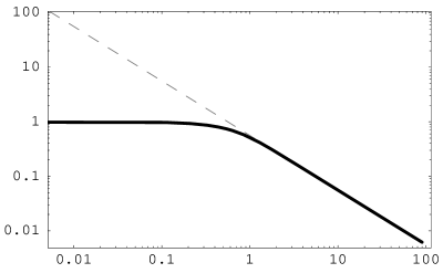
Figure 1: The solid line depicts $P(r)/r_{M}$ (on the vertical axis), wher $P$ is defined in (30), as a function of $r$ on the horizontal axis. The dashed line presents the function $0.28{r_{*}}/r$; The value of $r_{*}$ is set to 1 on this graph.

As in the AdSS case, the corrections to the Schwarzschild solution that are proportional to $m_{c}$ give rise to the four-dimensional Ricci curvature $R_{m_{c}}$. This is interesting since the curvature is completely due to the modification of gravity. However, unlike the AdSS case, this curvature is not a constant but depends on $r$; moreover it also depends on the strength of the source itself. The plot of the Ricci curvature is given on Fig. 2.

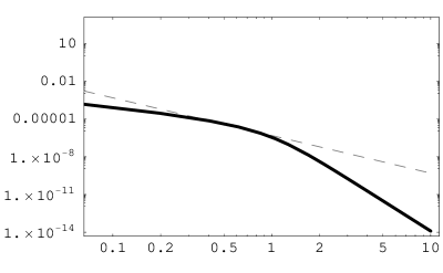
Figure 2: The solid line depicts the magnitude of the four-dimensional Ricci scalar curvature (on the vertical axes) as a function of $r$ on the horizontal axes. The dashed line depicts the dependence of the 4D Kretschmann scalar on $r$. The value of $r_{*}$ is set to 1 on this plot.

Similar to the AdSS solution the above properties can be expressed in terms of the invariants

$$R_{K}\,\gg R_{m_{c}}~{}~{}{\rm for}~{}~{}r\ll r_{*}~{}~{}{\rm and~{}for}~{}~{}r\gg r_{*}\,;~{}~{}{\rm while}~{}~{}R_{K}\,\sim R_{m_{c}}~{}~{}{\rm for}~{}~{}r\sim r_{*}\,.$$ (23)

Unlike in the AdSS solution, however, the curvature $R_{m_{c}}(r)$ decreases very fast after $r\gg r_{*}$. Hence, the induced curvature $R_{m_{c}}(r)$ is sub-dominant to $R_{K}$ everywhere except in the neighborhood of the point $r\sim r_{*}$ where both of these are of the same order $\sim m_{c}^{2}$, see Fig. 2.

Furthermore, unlike the AdSS solution, our solution can be presented in the same coordinate system even for $r\geq r_{c}$. This is because there is no horizon at $r=r_{c}$ and our solution smoothly turns into the 5D Schwarzschild solution

$$ds^{2}|_{y=0}\,=\,-\left(1\,-\,{{\tilde{r}}^{2}_{M}\over r^{2}}\right)\,dt^{2}\,+\,{dr^{2}\over\left(1\,-\,{{\tilde{r}}^{2}_{M}\over r^{2}}\right)}\,+\,r^{2}\,d\Omega_{2}^{2}\,.$$ (24)

The key property of this solution is that the gravitational radius is rescaled

$${\tilde{r}}_{M}\,\sim\,r_{M}\,\left({r_{c}\over r_{M}}\right)^{1/3}\,\gg\,r_{M}\,.$$ (25)

This has an explanation. The gravitational radius grows compared to $r_{M}$ because in the 5D regime the gravitational coupling constant grows. However, there is an opposite effect as well. In fact, the gravitational radius reduces compared to what it would have been in a pure 5D theory with no brane. This is because the effective mass of the source $M_{\rm eff}$, defined as ${\tilde{r}}_{M}^{2}\equiv M_{\rm eff}/M_{*}^{3}$, gets screened.

All the above results could be understood as follows. Consider an empty brane and an empty bulk. Minkowski space is a solution. Let us localize a static source on the brane at $r=0$. The Minkowski solution remains globally stable, however, the source, no matter how weak, triggers local instability of Minkowski space on a brane in the region $r\leq r_{*}$. In this patch Minkowski space is readjusted to a curved space. The curvature of the latter depends on the strength of the source, it slowly decreases with increasing $r$ but drops fast at $r>r_{*}$. For an observer at large distances it looks as if the source has polarized the medium (brane) around it. This observer measures the screened mass (25) which also includes the contributions of the curvature.

3.2 Solution in the bulk

At large enough distances, i.e. $\sqrt{r^{2}+y^{2}}\gg r_{*}$, the solution turns into a 5D spherically-symmetric Schwarzschild solution:

$$ds^{2}|_{\sqrt{r^{2}+y^{2}}\gg r_{*}}\,\sim\,-\left(1\,-\,{{\tilde{r}}^{2}_{M}\over r^{2}\,+\,y^{2}}\right)\,dt^{2}\,+\,{dr^{2}\over\left(1\,-\,{{\tilde{r}}^{2}_{M}\over r^{2}\,+\,y^{2}}\right)}\,+\,(r^{2}+y^{2})\,d\Omega_{3}^{2}\,.$$ (26)

However, the 5D spherical symmetric is only an approximation and does not hold for $\sqrt{r^{2}+y^{2}}\ll r_{*}$. In the latter regime the properties of the solution on and off the brane are rather different. The pure 5D spherically-symmetric solution (26) is squeezed both on and off the brane but it is more squeezed on the brane then in the bulk. Hence, the only symmetry of the solution that is left is the cylindrical symmetry.

4 The solutions

In this section we solve for $\lambda$ on the brane in the coordinate system (12).

From the (9) and (10) equations we deduce:

$$\gamma_{r}={\rm e}^{\lambda}\lambda_{y}~{},$$ (27)

and (9) and (11) can be rewritten as

$$2{\rm e}^{\lambda\over 2}P_{r} = {m_{c}r^{2}\over\sqrt{{\rm e}^{\lambda+\sigma}-\gamma^{2}}}\left((\lambda_{r}-{4\over r})\gamma-\gamma_{r}\right)~{},$$ (28)

$$r{\rm e}^{\lambda\over 2}P_{rr} = {2m_{c}r^{2}\over\sqrt{{\rm e}^{\lambda+\sigma}-\gamma^{2}}}\left((\lambda_{r}-{1\over r})\gamma-\gamma_{r}\right)~{},$$ (29)

where we have defined

$$P(r)\,\equiv\,r\,(1\,-\,{\rm exp}(-\lambda))\,.$$ (30)

Using (28) and (29) in the $yy$ equation of motion (7) we obtain:

$$0=6m_{c}^{2}r^{2}(2Q+rQ_{r})+r^{2}Q_{r}^{2}-8rQQ_{r}+4Q^{2}~{}.$$ (31)

where $Q=P_{r}$. Let us study this equation. First of all we note that the quadratic terms in (31) can only be neglected when $r$ is large. This suggests that the naive linearized approximation that neglects the quadratic terms is viable only for large distances, no matter how weak the source is. Hence, for $r\gg m_{c}^{-1}$ we can neglect the last three terms on the r.h.s. of (31) and then the solution is

$$P={{\tilde{r}}_{M}^{2}\over r}+C_{1}~{},$$ (32)

where ${\tilde{r}}_{M}$ and $C_{1}$ are integration constants. $C_{1}=0$ gives the 5D Schwarzschild solution of radius ${\tilde{r}}_{M}$. In a similar fashion, for $r\ll m_{c}^{-1}$ we can neglect the term proportional to $m_{c}^{2}$ in (31). The solutions in this case are

$$P=r_{M}+C_{2}r^{2(2\pm\sqrt{3})+1}~{},$$ (33)

where $r_{M}$ and $C_{2}$ are integration constants. In this case, $C_{2}=0$ gives the 4D Schwarzschild solution of radius $r_{M}$.

We will show that there is an interpolating solution between these two regimes (regular branch) together with a second solution that becomes 5D de Sitter Schwarzschild at large distances (accelerated branch). In order to find these exact solutions let us rewrite (31) as

$$0=U_{z}^{2}-4(1+U)U_{z}-8U(2+U)~{},$$ (34)

where $z={\rm ln}(r/r_{0})$ and $U=-2{\rm exp}(-2z)Q/3m_{c}^{2}r_{0}^{2}$ ($r_{0}$ an arbitrary constant). There are two solutions that are given implicitly by:

$${\rm ln}\left[-{(1+3U+f)\over U^{2}(3+3U+\sqrt{3}f)^{2\sqrt{3}}(-5-3U+f)}\right] = 8z+C_{3}~{},$$ (35)

$${\rm ln}\left[-{(-5-3U+f)(-3-3U-\sqrt{3}f)^{2\sqrt{3}}\over(U+2)^{2}(1+3U+f)}\right] = 8z+C_{3}~{},$$ (36)

where $f=\sqrt{1+6U+3U^{2}}$ and $C_{3}$ an integration constant.

Let us first consider the solution (35). For $U>0$ the left hand side is a decreasing function of $U$. To obtain the large distance ($r\gg r_{*}$) behavior of the solution we consider the limit $U\rightarrow 0^{+}$ ($z\rightarrow+\infty$) in which (35) reads

$${\rm ln}~{}U=-4z+C_{4}+{\cal O}(U)~{},$$ (37)

that gives (32) upon integration. The short distance regime ($r\ll r_{*}$) is found by taking the limit $U\rightarrow+\infty$ ($z\rightarrow-\infty$). In this case (35) is given by

$$(1+\sqrt{3}){\rm ln}~{}U=-4z+C_{5}+{\cal O}\left({1\over U}\right)~{},$$ (38)

that reproduces the asymptotic behavior of (33) (with the minus sign). Thus, we have found a smooth solution that interpolates between the 4D and 5D Schwarzschild solutions on the brane. This corresponds to the regular branch.

Let us now study the second solution (36). For $U<-2$ the left hand side of (36) is an increasing function of $U$. In the large distance limit $U\rightarrow-2^{-}$ ($z\rightarrow+\infty$) (36) reads

$${\rm ln}(-U-2)=-4z+C_{4}+{\cal O}(U+2)~{},$$ (39)

that gives upon integration

$$P={{\tilde{r}}_{M}^{2}\over r}+m_{c}^{2}r^{3}~{},$$ (40)

where we have absorbed the integration constant $C_{4}$ in the definition of $\tilde{r}_{M}$. This is the 5D de Sitter-Schwarzschild solution of the accelerated branch. The short distance behavior is obtained by considering the $U\rightarrow-\infty$ ($z\rightarrow-\infty$) of (36). This gives

$$(1+\sqrt{3}){\rm ln}(-U)=-4z+C_{5}+{\cal O}\left({1\over U}\right)~{}.$$ (41)

The above equation gives the following behavior of the potentials for $r_{M}\ll r\ll r_{*}$

$$\nu\,=\,-\lambda\,\simeq\,-\,{r_{M}\over r}\,-\,0.84\,m_{c}^{2}\,r^{2}\left({r_{*}\over r}\right)^{2(\sqrt{3}-1)}.$$ (42)

Below we derive in detail the relation between the mass of the source that determines the 4D Schwarzschild radius $r_{M}$ and the “screened” mass that determines the 5D Schwarzschild behavior (with radius $\widetilde{r}_{M}$) at large distances ($r\gg r_{c}$). In order to do that let us rewrite (35) as

$$F(U)=ku~{},$$ (43)

by defining the variable $u=r^{3}$, the constant $k={\rm exp}(3C_{3}/8)/r_{0}^{3}$ and

$$F(U)=\left({(1+3U+f)\over U^{2}(3+3U+\sqrt{3}f)^{2\sqrt{3}}(5+3U-f)}\right)^{3/8}~{}.$$ (44)

$F(U)$ is a monotonically decreasing function for $U>0$ that diverges in the limit $U\rightarrow 0+$ and vanishes in the limit $U\rightarrow+\infty$. Note that $U=-2P_{u}/m_{c}^{2}$. On the other hand, (43) gives $U=F^{-1}(ku)$. Therefore

$$-{2\over m_{c}^{2}}\int^{\infty}_{0}P_{u}{\rm d}u={1\over k}\int^{\infty}_{0}F^{-1}(ku){\rm d}(ku)~{},$$ (45)

where the integral on the right hand side is equivalent to the following integral

$$\int^{\infty}_{0}F(U){\rm d}U\approx 0.43~{}.$$ (46)

Imposing the asymptotic behavior of $P$: $P(0)=r_{M}$ and $P(+\infty)=0$ on (45) gives

$$2kr_{M}=0.43m_{c}^{2}$$ (47)

In turn, the large distance behavior of $P$: $P\sim\widetilde{r}_{M}^{2}/r$ obtained from (35) gives

$$k(\widetilde{r}_{M}r_{c})^{3/2}=\left({3\over 4\sqrt{2}(3+\sqrt{3})^{\sqrt{3}}}\right)^{3/4}\approx 0.082~{}.$$ (48)

Thus, from (45) and (48) we obtain the exact relation between the 4D and 5D Schwarzschild radii:

$$r_{M}=2.6~{}\widetilde{r}_{M}\sqrt{\widetilde{r}_{M}\over r_{c}}~{}.$$ (49)

The 4D Ricci curvature $R_{4}$ can be readily calculated using the expression:

$$R_{4}=-{3\over 2}m_{c}^{2}(U_{z}+4U)\,.$$ (50)

It goes to zero in the large r limit (in the regular branch) and grows as one approaches the source at small $r$. Moreover, it gives rise to the properties described in the previous section.

In this gauge we solve for the combination of $\gamma$ and $\sigma$ at $y=0^{+}$ which takes the form

$${\rm e}^{-{\sigma\over 2}}\gamma={\rm arctan}\left({rP_{rr}-4P_{r}\over 6m_{c}r}\right)={\rm arctan}\left({m_{c}r_{0}\over 4}{\rm e}^{z}(2U-U_{z})\right)~{}.$$ (51)

The latter expression will be used in the next section to check the continuity of the solution in the $m_{c}\to 0$ limit.

5 No vDVZ discontinuity

The vDVZ discontinuity [9, 10] is an interesting observation that the theory in the $m_{c}\to 0$ limit could differ from the one in which $m_{c}=0$ is set ab initio (i.e., from the Einstein theory). Below we will argue that the vDVZ observation is based on arguments that do not hold when the dynamical effects of the mass screening are taken into account.

We will show that our solution is continuous in the $m_{c}\to 0$ limit. We present these arguments it two different ways. First let us look at the solution of the previous section. In the limit $m_{c}\to 0$ (i.e. $r_{c}\to\infty$) we find:

$$r_{*}\to\infty\,;~{}~{}~{}{\tilde{r}}_{M}\to\infty\,;~{}~{}~{}M_{\rm eff}\to 0\,.$$ (52)

Moreover, the off-diagonal term in the solution behaves as follows:

$$\gamma e^{-\sigma/2}|_{r\gg r_{c}}\,\simeq\,{\rm arctan}\left({{\tilde{r}}_{M}^{2}\over m_{c}r^{3}}\right)\,\ll 1\,,$$ (53)

which is always small and the regime of the applicability of the above expression goes to infinity in the limit $m_{c}\to 0$. Moreover, in the region $r\ll r_{*}$ we get

$$\gamma e^{-\sigma/2}|_{r\ll r_{*}}\,\to\,{\rm arctan}\left({m_{c}\over m_{c}^{8\over 3(1+\sqrt{3})}}\right)\,\to 0\,.$$ (54)

Based on the above findings we conclude that the solution turns into an exactly 4D Schwarzschild solution in the $m_{c}\to 0$ limit. The regions where it could deviate from the 4D solution, $r\gg{\rm min}\{r_{*},r_{c}\}$, go to infinity.

The vDVZ discontinuity was originally formulated in [9, 10] in terms of a one-graviton exchange amplitude. It is instructive to see the loophole in this formalism as well. The arguments of [9, 10] go as follows. The momentum space amplitude for one graviton exchange between the source of a stress-tensor $T^{\rm source}_{\mu\nu}$ and a probe $T^{\prime}_{\mu\nu}$ is given by

$${\cal A}_{m}\,=\,{1\over M_{\rm Pl}^{2}}\,{T^{\rm source}_{\mu\nu}\,T^{\prime\mu\nu}\,-\,{1\over 3}\,T^{\rm source}\,T^{\prime}\,\over p^{2}\,+\,m_{c}\,p+i{\epsilon}}\,.$$ (55)

(Here $T$’s denote the trace of the stress-tensors.) The very same amplitude for massless 4D gravity is

$${\cal A}_{0}\,=\,{1\over M_{\rm Pl}^{2}}\,{T^{\rm source}_{\mu\nu}\,T^{\prime\mu\nu}\,-\,{1\over 2}T^{\rm source}\,T^{\prime}\over p^{2}+i{\epsilon}}\,.$$ (56)

Hence, in the limit $m_{c}\to 0$ Eq. (55) does not reduce to Eq. (56). This is the vDVZ discontinuity.

Our exact solution suggests that these arguments do not hold in an intricate way. Let us start with $r\gg r_{*}$. In this region the linearized equations turn into source-free equations since the source is only localized at distances $r\ll r_{*}$. The source-free equations can be solved and the solution is a 5D Schwarzschild metric with the Schwarzschild radius being a yet unspecified integration constant. This constant should either be fixed by matching to the solution at $r\leq r_{*}$, or by calculating the ADM mass. In either case the curvature created by the source will also contribute to the ADM mass. Therefore, at large distances where the perturbative one-graviton exchange is believed to be a good approximation, we have to replace a source $T^{\rm source}_{\mu\nu}$ with an effective source $T^{\rm eff}_{\mu\nu}$ that takes into account the fact that the source distorts the medium around it. This can be achieved by making a substitution $r_{c}\to r_{*}$ in (55). In the case of a static source of mass $M$, this would replace its mass by an effective mass (3). Once this replacement is done, we find that the tree level amplitude is discontinuous, however, this is not problematic because simultaneously the region in which the expression (55) is applicable, i.e. $r\gg r_{*}$, goes to infinity according to (52). Hence, no vDVZ discontinuity remains in the theory.

We also note that although the solution is nonperturbative, nevertheless the fields in the metric remain weak (much smaller than 1) all the way down to distances $r\geq r_{M}$. Hence, the solution that we find never exhibits the strong field behavior as long as $r\geq r_{M}$; this is similar to the conventional 4D Schwarzschild solution of massless gravity.

6 Weak-field versus $G_{N}$-expansion

Consider small perturbations $h$ about a flat metric $\eta$

$$g_{\mu\nu}\,=\,\eta_{\mu\nu}\,+\,h_{\mu\nu}\,.$$ (57)

The weak-field expansion (WFE) is a power series expansion in $h\ll 1$. In conventional Einstein’s theory the WFE coincides with an expansion in Newton’s coupling $G_{N}$. However, in the DGP model this is not so because there is another dimensionfull parameter in the theory, $m_{c}$, that contaminates the $G_{N}$-expansion. To see this in some detail let us first look at the WFE and $G_{N}$-expansion in Einstein’s theory. This can be done in the Lagrangian or in equations of motion. We choose the former. Ignoring the indexes that are not important for our purposes, the WFE of the Einstein Lagrangian reads:

$$M_{\rm Pl}^{2}\,\left(h\,\partial^{2}\,h\,+\,h\,\partial\,h\,\partial\,h\,+...\right)+h\,T\,,$$ (58)

where the dots denote terms that contain only two derivatives but higher powers of $h$. The last term in (58) describes the interactions of gravity with matter. The expansion in the parenthesis of (58) in powers of dimensionless field $h$ is acceptable as long as $h\ll 1$ . One the other hand, one could rescale the field $h\to{\tilde{h}}/M_{\rm Pl}$. Then the Lagrangian takes the form

$$\left({\tilde{h}}\,\partial^{2}\,{\tilde{h}}\,+\,\sqrt{G_{N}}\,{\tilde{h}}\,\partial\,{\tilde{h}}\,\partial\,{\tilde{h}}\,+...\right)\,+\,\sqrt{G_{N}}\,{\tilde{h}}\,T\,.$$ (59)

The rescaled field ${\tilde{h}}$ has the canonical dimensionality. The Newton constant emerges only in the graviton interaction vertices. Therefore, one can develop the standard Feynman diagram technique as an expansion in powers of $G_{N}$. The results of this expansion would coincide with the results of the WFE.

The above arguments do not hold in general in theories where gravity gets modified at some large distance scale $r_{c}$. This is because the new dimensionfull parameter $r_{c}=m_{c}^{-1}$ enters the expansions. Below we concentrate on the DGP model to discuss this issue. The 4D part of the Lagrangian in the DGP model can schematically be written as follows:

$$M_{\rm Pl}^{2}\,\left(h\,\partial^{2}\,h\,+\,h\,\partial\,h\,\partial\,h\,+...\right)\,+\,m_{c}\,M_{\rm Pl}^{2}\,\left(h\,\partial\,h\,+\,h\,h\,\partial\,h\,+\,...\right)\,+\,h\,T\,.$$ (60)

Let as look at the two terms in (60). The cubic and higher powers in the first parenthesis can be neglected w.r.t. the quadratic terms as long as $h\ll 1$. Likewise, the cubic and higher powers in the second parenthesis can be neglected w.r.t. the quadratic terms as long as $h\ll 1$. However, the cubic term in the first parenthesis cannot be neglected w.r.t. the quadratic terms in the second parenthesis unless the derivative of the filed is very small $\partial h\ll m_{c}$. To see why this is important one should look at the trace equation (since we dropped the indices in all the expressions above we have not made a distinction between the traceless and trace Einstein equations). The trace equation is subtle because the linearized bulk equations make the coefficient of the first quadratic term in (60) vanish identically and the nonlinear term is the leading one [22]. Therefore, at short distances $\partial h\gg m_{c}$ some of the nonlinear terms in (60) cannot be neglected. This is despite of the fact that the fields are weak ($h\ll 1$)!

Let us now turn to the $G_{N}$-expansion of (60). It is clear that the rescaling $h\to{\tilde{h}}/M_{\rm Pl}$ does not lead to a Lagrangian with a single dimensionfull coupling as in (59). Instead we get the nonlinear vertices that contain $G_{N}$ as well as $m_{c}$. This leads to dramatic consequences. Certain nonlinear but tree-level Feynman diagrams contain inverse powers of $m_{c}$ and diverge in the $m_{c}\to 0$ limit [2]. For finite $m_{c}$ the same diagrams give rise to the breakdown of the $G_{N}$-expansion below the scale $r_{*}$ [2]. However, this is an artificial difficulty that is brought about by the expansion in $G_{N}$. As we have seen in the previous sections the exact solution is regular in the $m_{c}\to 0$ limit and fields are weak as log as $r\gg r_{M}$. The metric is non-analytic in $G_{N}$ showing that the $G_{N}$-expansion is not valid even in the regions where it naively would be expected to work. Nevertheless, as we discussed in the first section, the problems with the $G_{N}$ expansion can be fixed. Classically this is achieved by summing up the nonlinear corrections [2]. In the quantum theory things are more subtle since the summation of the diagrams is hard to perform while the expansion in $G_{N}$ can lead to the appearance of certain higher-dimensional operators that are suppressed by unacceptably low scale [15]. However, as was shown in [7] and discussed in section 1, even in this case one can formulate a quantum perturbation theory in $G_{N}$ in which the counter-terms eliminate the dangerous loop-induced operators and the $G_{N}$-expansion remains a useful tool.

Note that a slight modification of the model can give rise to a theory in which the $G_{N}$-expansion does not break down below $r_{*}$ [22]. In this case the calculations can be performed straightforwardly as in the Einstein theory. It remains to be see if the approach of Ref. [22] can be implemented in a full nonlinear theory.

7 Existence of the bulk solution

In the previous sections we presented an exact solution for the metric and extrinsic curvature on the brane. Below this will be used to argue that the solutions can be smoothly continued into the whole bulk. For this we use the ADM formalism [24].

We introduce the lapse scalar field ${\cal N}$, and the shift vector field ${\cal N}_{\mu}$ according to the standard rules:

$$g_{\mu y}\,\equiv\,{\cal N}_{\mu}\,,~{}~{}~{}g_{yy}\,\equiv\,{\cal N}^{2}\,+\,g_{\mu\nu}\,{\cal N}^{\mu}\,{\cal N}^{\nu}\,.$$ (61)

After integration by parts the action (5) takes the form:

$$S=M_{*}^{3}\int d^{4}xdy\sqrt{-{\rm det}g_{\mu\nu}}\,{\cal N}\,\left(\widetilde{R}\,+\,K^{2}-K_{\mu\nu}K^{\mu\nu}\right)\,+\,M_{P}^{2}\int d^{4}x\,\sqrt{-\widetilde{g}}\widetilde{R}~{},$$ (62)

where $K=g^{\mu\nu}K_{\mu\nu}$ is the trace of the extrinsic curvature

$$K_{\mu\nu}\,=\,{1\over{\cal N}}\,\left(\partial_{y}g_{\mu\nu}-D_{\mu}{\cal N}_{\nu}-D_{\nu}{\cal N}_{\mu}\right)\,,$$ (63)

and $D_{\mu}$ is a covariant derivative with the metric $g_{\mu\nu}$. Note that the Gibbons-Hawking term implied in (5) is canceled in (62) after integration by parts.

What we found in the previous section are the quantities:

$$g_{\mu\nu}(x,y=0)\,=\,{\widetilde{g}}_{\mu\nu}(x)\,~{}~{}~{}~{}{\rm and}~{}~{}~{}~{}K_{\mu\nu}(x,y=0)\,.$$ (64)

This data on a brane can be considered as an initial data from which the metric and extrinsic curvature in the bulk could be reconstructed. Let us look at the bulk equations of motion that follow from (62) by taking variations w.r.t. ${\cal N}$, ${\cal N}_{\mu}$ and $g^{\mu\nu}$ we get respectively

$$\widetilde{R}\, = \,K^{2}-K_{\mu\nu}^{2}\,,$$ (65)

$$D_{\mu}K\, = \,D^{\nu}K_{\mu\nu}\,,$$ (66)

$$g_{\lambda\mu}g_{\beta\nu}{1\over d}\partial_{y}(d(Kg^{\lambda\beta}-K^{\lambda\beta}))\, = \,-{\cal N}G_{\mu\nu}+{1\over 2}g_{\mu\nu}{\cal N}(K^{2}-K_{\beta\lambda}^{2})+D_{\mu}D_{\nu}{\cal N}$$ (67)

$$\hskip-147.95424pt-g_{\mu\nu}D^{2}{\cal N}+2D_{[\lambda}(K^{\lambda}_{\nu]}{\cal N}_{\mu})+g_{\mu\nu}D^{\lambda}(K_{\nu\lambda})-D^{\lambda}({\cal N}_{\lambda}K_{\mu\nu})+2{\cal N}K^{\lambda}_{[\mu}K_{\nu]\lambda}\,,$$

where $d\equiv\sqrt{-{\rm det}g_{\mu\nu}}$ and $G_{\mu\nu}$ denotes the Einstein tensor. We look at (65 -67) as at a system of differential equations in the $y$ variable. Then, Eq. (65) is just an algebraic equation since it contains no $y$ derivatives except those that are already reabsorbed into the definition of $K$. The same is true for Eq. (66). Furthermore, it is not difficult to check that (65) is satisfied at $y=0+$ if (28)-(31) are fulfilled. Moreover, Eq. (66), when considered as an equation defining $\gamma_{y}(r,y=0+)$, is satisfied by our solution at $y=0+$. Hence, the only true differential equation which evolves the initial data into the bulk is (67) that contains first derivative w.r.t. $y$ on its l.h.s.

Given the initial value formulation (65)-(67) local existence of the bulk solution is guaranteed [25, 26]. The problem of global existence of the bulk solution, i.e. the geodesic completeness of the bulk solution obtained by the evolution equation (67), is not easy to establish in general. However, in the present context we can take an advantage of the fact that the bulk metric asymptotes to Minkowski space. Indeed, a number of theorems exist for asymptotically flat spaces (see [27]). In particular, in [27] the evolution along a timelike direction of data given on a 3 dimensional surface is shown to be smooth and geodesically complete under the assumption of strong asymptotic flatness and a smallness condition on the initial data. The smallness condition is:

$${\rm sup}\left((d_{0}^{2}+1)^{3}R_{\mu\nu}^{2}\right)+\int\sum_{l=0}^{3}(d_{0}^{2}+1)^{l+1}\nabla^{l}K^{2}+\int\sum_{l=0}^{1}(d_{0}^{2}+1)^{l+3}\nabla^{l}B^{2}<\infty\,,$$ (68)

where $d_{0}$ is the geodesic distance from a point $o$ in the initial data surface and $B$ is the curl of the traceless part of $R_{\mu\nu}$. Our initial data is strongly asymptotically flat since

$$\widetilde{g}_{\mu\nu} = (1+{\tilde{r}_{M}^{2}\over r^{2}})\delta_{\mu\nu}+{\cal O}(r^{-{5\over 2}})\,,$$

$$K_{\mu\nu} = {\cal O}(r^{-{7\over 2}})\,,$$

for sufficiently large $r$, and satisfies the smallness condition as well. This suggests that the solution can be extended into a smooth, geodesically complete and asymptotically flat bulk, however, does not constitute a full proof.

We also mention that one could easily find a linearized form of the solution at $r\gg r_{c}$. This solution coincides with the linearized 5D Schwarzschild metric in which the integration constant is fixed to the screened mass, i.e., ${\tilde{r}}_{M}^{2}=r_{*}\,r_{M}$.

8 Concluding remarks

In this section we discuss certain interesting issues that arise as a byproduct of our studies and for which further detailed work is needed.

(i) Geodesic motion of matter and light. It is interesting to look at the geodesic motion of matter and light in the metric (12). The geodesic equation for the light rays propagating on the brane is $dr/dt=e^{\lambda}$. The useful form of $\lambda$ is given in Eq. (20). From this we conclude that for $r\mathrel{\hbox to0.0pt{\lower 3.0pt\hbox{\hskip 0.0pt$\sim$}\hss}\raise 1.0pt\hbox{$<$}}r_{*}$ the light propagates on the brane as it would in conventional 4D Einstein gravity with some corrections that are negligible everywhere except in the region $r\sim r_{*}$. As we discussed, for a solar mass object this distance is at $10^{20}$ cm and the above effect will be overshadowed by gravitational effects of other sources.

The matter geodesics are more complicated however. The 5D geodesic equation on the brane contains derivatives of $\gamma$ across the brane that multiply $dy$. Since the $\gamma_{y}$ is singular on the brane, it can give rise to finite contributions even though it is multiplied by the vanishing differentials. If so, the motion of 5D matter will get additional contributions from the extrinsic curvature of the brane. Also we could not manage to solve the matter geodesic equations, it looks like that the extrinsic curvature part is canceling, according to (4), the modifications of 4D gravity that appear in $\lambda$. On the other hand, 4D geodesics for localized matter in 4D are determined by the 4D induced metric governed by $\lambda$.

(ii) Comments on Black Holes. In the present work we were dealing with a macroscopic source on the brane, a star for instance. In the context of the DGP model these type of sources are assumed to be localized on a brane by a certain mechanism not related to gravity itself. If the sources were not localized, then, as is known [28], the brane with the induced graviton kinetic term has effectively repulsive gravity and it would push any source off the brane. For instance, ordinary black holes cannot be held on the brane. However, charged black holes could still be quasi-localized if the corresponding gauge fields are localized. It would be interesting to see how the properties of charged black holes would differ. It is also very interesting to understand in detail the structure of the horizon of a black hole in the bulk. Our preliminary findings suggest that it should have a cylindrical form, where the cylinder extends from a brane into the bulk to a distance that is bigger that ${\tilde{r}}_{M}$ but smaller than $r_{*}$. Further detailed investigations are needed to understand the validity and implications of these observations.

References

- [1] G. Dvali, G. Gabadadze and M. Porrati, Phys. Lett. B485, 208 (2000) [hep-th/0005016].
- [2] C. Deffayet, G. R. Dvali, G. Gabadadze and A. I. Vainshtein, Phys. Rev. D 65, 044026 (2002) [hep-th/0106001].
- [3] A. Gruzinov, [arXiv:astro-ph/0112246].
- [4] M. Porrati, Phys. Lett. B 534, 209 (2002) [arXiv:hep-th/0203014].
- [5] A. Lue and G. Starkman, Phys. Rev. D 67, 064002 (2003) [arXiv:astro-ph/0212083].
- [6] C. Middleton and G. Siopsis, arXiv:hep-th/0311070.
- [7] A. Nicolis and R. Rattazzi, [arXiv:hep-th/0404159].
- [8] A. I. Vainshtein, Phys. Lett. 39B, 393 (1972).
- [9] H. van Dam and M. J. Veltman, Nucl. Phys. B 22, 397 (1970).
- [10] V. I. Zakharov, JETP Lett. 12, 312 (1970)
- [11] I. I. Kogan, S. Mouslopoulos and A. Papazoglou, Phys. Lett. B 503, 173 (2001) [arXiv:hep-th/0011138].
- [12] M. Porrati, Phys. Lett. B 498, 92 (2001) [arXiv:hep-th/0011152].
- [13] G. Dvali, A. Gruzinov and M. Zaldarriaga, Phys. Rev. D 68, 024012 (2003) [arXiv:hep-ph/0212069].
- [14] N. Arkani-Hamed, H. Georgi and M. D. Schwartz, Annals Phys. 305, 96 (2003) [arXiv:hep-th/0210184].
- [15] M. A. Luty, M. Porrati and R. Rattazzi, JHEP 0309, 029 (2003) [arXiv:hep-th/0303116].
- [16] V. A. Rubakov, [arXiv:hep-th/0303125].
- [17] G. Dvali, [arXiv:hep-th/0402130].
- [18] C. Deffayet, Phys. Lett. B 502, 199 (2001) [arXiv:hep-th/0010186].
- [19] C. Deffayet, G. R. Dvali and G. Gabadadze, Phys. Rev. D 65, 044023 (2002) [arXiv:astro-ph/0105068].
- [20] G. Gabadadze and M. Shifman, arXiv:hep-th/0312289.
-
[21]
M. Porrati and J. W. Rombouts,
arXiv:hep-th/0401211;
M. Kolanovic, M. Porrati and J. W. Rombouts, Phys. Rev. D 68, 064018 (2003) [arXiv:hep-th/0304148]. - [22] G. Gabadadze, [arXiv:hep-th/0403161].
- [23] G. W. Gibbons and S. W. Hawking, Phys. Rev. D 15 (1977) 2738.
- [24] R. Arnowitt, S. Deser, C. W. Misner, ”Gravitation: an introduction to current research”, Louis Witten ed. (Wiley 1962), chapter 7, pp 227–265; [arXiv:gr-qc/0405109].
- [25] R. Wald, “General Relativity”, Chicago University Press, 1984.
- [26] E. Anderson and R. Tavakol, [arXiv:gr-qc/0309063].
- [27] S. Klainerman and F. Nicolo, “The Evolution Problem in General Relativity”, Birkhauser Boston (2002); Class. Quantum Grav. 16 (1999) R73-R157.
- [28] M. Kolanovic, Phys. Rev. D 65, 124005 (2002) [arXiv:hep-th/0203136].