Quasinormal behavior of massless scalar field perturbation
in Reissner-Nordström anti-de Sitter spacetimes

Abstract

We present a comprehensive study of the massless scalar field perturbation in the Reissner-Nordström anti-de Sitter (RNAdS) spacetime and compute its quasinormal modes (QNM). For the lowest lying mode, we confirm and extend the dependence of the QNM frequencies on the black hole charge got in previous works. In near extreme limit, under the scalar perturbation we find that the imaginary part of the frequency tends to zero, which is consistent with the previous conjecture based on electromagnetic and axial gravitational perturbations. For the extreme value of the charge, the asymptotic field decay is dominated by a power-law tail, which shows that the extreme black hole can still be stable to scalar perturbations. We also study the higher overtones for the RNAdS black hole and find large variations of QNM frequencies with the overtone number and black hole charge. The nontrivial dependence of frequencies on the angular index $\ell$ is also discussed.

I Introduction

It is well known that under perturbations the surrounding geometry of a black hole will experience damped oscillations with frequencies and damping times entirely determined by the black hole parameters. These oscillations are called “quasinormal modes” (QNM). They carry unique fingerprints of black holes which would lead to the direct identification of the black hole existence. Due to the potential astrophysical interest, extensive study of QNM of black holes in asymptotically flat spacetimes have been performed for the last few decades (for comprehensive reviews see Nollert-99 ; Kokkotas-99 and references therein). Considering the case when the black hole is immersed in an expanding universe, the QNMs of black holes in de Sitter space have also been investigated deSitter_1 ; deSitter_2 .

Motivated by the recent discovery of the anti-de Sitter/conformal field theory (AdS/CFT) correspondence, the investigation of QNMs in anti-de Sitter (AdS) spacetimes became appealing in the past years. It was argued that the QNMs of AdS black holes have direct interpretation in terms of the dual conformal field theory. The first study of the QNMs in AdS spaces was performed by Chan and Mann Chan_Mann . Subsequently, Horowitz and Hubeny suggested a numerical method to calculate the QN frequencies directly and made a systematic investigation of QNMs for scalar perturbation on the background of Schwarzschild AdS (SAdS) black holes Horowitz-00 . Considering that the RNAdS solution provides a better framework than the SAdS geometry and may contribute significantly to our understanding of space and time, the Horowitz-Hubeny numerical method was generalized to the study of QNMs of RNAdS black holes in Wang-00 and later crosschecked by using the time evolution approach Wang-01 . In addition to the scalar perturbation, gravitational and electromagnetic perturbations in AdS black holes have also attracted attention Cardoso ; Berti-03 . Other works on QNMs in AdS spacetimes can be found in Konoplya-02 ; Birmingham ; Zhu_Wang_Mann_Abdalla ; AdS_SeveralAuthors ; Cardoso_Lemos ; Cardoso_Konoplya_Lemos .

Recently in Berti-03 Berti and Kokkotas used the frequency-domain method and restudied the scalar perturbation in RNAdS black holes. They verified most of our previous numerical results in Wang-00 ; Wang-01 , however, disapproved the property of the real part of the QN frequency with the increase of the black hole charge. Our first aim in this paper is to check their results by using both improved Horowitz-Hubeny method and time evolution approach.

As was pointed out in Wang-00 and later supported in Berti-03 , the Horowitz-Hubeny method breaks down for large values of the charge. To study the QNMs in the near extreme and extreme RNAdS backgrounds, we need to count on time evolution approach. Employing an improved numerical method, we will show that the problem with minor instabilities in the form of “plateaus”, which were observed in Wang-01 , is overcome. We obtain the precise QNMs behavior in the highly charged RNAdS black holes.

In addition to the study of the lowest lying QNMs, it is interesting to study the higher overtone QN frequencies for scalar perturbations. The first attempt was carried out in Cardoso_Konoplya_Lemos . In the present work we would like to extend the study to the RNAdS backgrounds.

It was argued that the dependence of the QN frequencies on the angular index $\ell$ is extremely weak Berti-03 . This was also claimed in Cardoso_Konoplya_Lemos . Using our numerical results we will show that this weak dependence on the angular index is not trivial.

The plan of the paper is as follows. In Sec.II we review the background metric, display the scalar wave equations and briefly present our numerical methods. In Sec.III we describe in detail our numerical results. The conclusions and discussions will be presented in Sec.IV.

II Equations and numerical methods

II.1 Geometry and fields

The metric describing a charged, asymptotically anti-de Sitter spherical black hole, written in spherical coordinates, is given by

$$ds^{2}=-h(r)dt^{2}+h(r)^{-1}dr^{2}+r^{2}(d\theta^{2}+\sin^{2}\theta d\phi^{2})\ ,$$ (1)

where the function $h(r)$ is

$$h(r)=1-\frac{2m}{r}+\frac{Q^{2}}{r^{2}}-\frac{\Lambda r^{2}}{3}\ .$$ (2)

We are assuming a negative cosmological constant, usually written as $\Lambda=-3/R^{2}$. The integration constants $m$ and $Q$ are the black hole mass and electric charge respectively. The extreme value of the black hole charge, $Q_{max}$, is given by the function of the event horizon radius in the form $Q_{max}^{2}=r_{+}^{2}(1+3r_{+}^{2}/R^{2})$.

The spacetime causal structure depends on the zeros of $h(r)$. Changing the parameters $m$, $Q$ and $R$, the function $h(r)$ may have none, one, or two positive zeros. In the Reissner-Nordström-anti-de Sitter case, $h(r)$ has two simple real, positive roots ($r_{+}$ and $r_{-}$) and two complex roots ($r_{1}$ and $r_{1}^{*}$, asterisk denoting complex conjugation). In the so-called extreme Reissner-Nordström-anti-de Sitter case, $h(r)$ has one double positive zero (also denoted $r_{+}$) and two complex roots ($r_{1}^{ext}$ and $\left(r_{1}^{ext}\right)^{*}$). The horizons $r_{-}$ and $r_{+}$ with $r_{-}<r_{+}$, are called Cauchy and event horizons, respectively. In this work we will treat the dynamics of fields in the black hole exterior, the submanifold given by the patch $T_{+}=\left\{(t,r,\theta,\phi),r>r_{+}\right\}$.

In the region $T_{+}$, we define a “tortoise coordinate” $r^{*}(r)$ in the usual way,

$$r^{*}(r)=\int\frac{dr}{h(r)}\,\,.$$ (3)

Assuming $h(r)$ has two distinct positive roots (nonextreme case), the tortoise coordinate is given by

$$r^{*}(r)=\frac{1}{2\kappa_{+}}\ln\left(r-r_{+}\right)-\frac{1}{2\kappa_{-}}\ln\left(r-r_{-}\right)\\ -A\ln(r^{2}+pr+q)+\frac{2(B+Ap)}{\sqrt{4q-p^{2}}}\\ \times\left[\arctan\left(\frac{2r+p}{\sqrt{4q-p^{2}}}\right)-\frac{\pi}{2}\right]\,\,,$$ (4)

with the constants $\kappa_{+}$, $\kappa_{-}$, $A$, $B$, $p$ and $q$ given by

$$\frac{1}{2\kappa_{+}}=\frac{R^{2}r_{+}^{2}}{(r_{+}-r_{-})(3r_{+}^{2}+r_{-}^{2}+2r_{+}r_{-}+R^{2})}\,\,,$$ (5)

$$\frac{1}{2\kappa_{-}}=\frac{R^{2}r_{-}^{2}}{(r_{+}-r_{-})(3r_{-}^{2}+r_{+}^{2}+2r_{+}r_{-}+R^{2})}\,\,,$$ (6)

$$A=\frac{R^{2}(r_{+}+r_{-})(r_{+}^{2}+r_{-}^{2}+2r_{+}r_{-}+R^{2})}{2(3r_{+}^{2}+r_{-}^{2}+2r_{+}r_{-}+R^{2})(3r_{-}^{2}+r_{+}^{2}+2r_{+}r_{-}+R^{2})}\,\,,$$ (7)

$$B=\frac{R^{2}(r_{+}^{2}+r_{-}^{2}+R^{2})(r_{+}^{2}+r_{-}^{2}+r_{+}r_{-}+R^{2})}{(3r_{+}^{2}+r_{-}^{2}+2r_{+}r_{-}+R^{2})(3r_{-}^{2}+r_{+}^{2}+2r_{+}r_{-}+R^{2})}\,\,,$$ (8)

$$p=r_{+}+r_{-}\,\,,\,\,q=R^{2}+r_{+}^{2}+r_{-}^{2}+r_{+}\,\,.$$ (9)

The constant of integration in the expression (4) was chosen so that $\lim_{r\rightarrow\infty}r^{*}(r)=0$.

Consider now a scalar perturbation field $\Phi$ obeying the massless Klein-Gordon equation

$$\Box\Phi=0\ .$$ (10)

The usual separation of variables in terms of a radial field and a spherical harmonic $\textrm{Y}_{\ell,m}(\theta,\varphi)$,

$$\Phi=\sum_{\ell\,m}\frac{1}{r}\Psi(t,r)\textrm{Y}_{\ell m}(\theta,\phi)\ ,$$ (11)

leads to Schrödinger-type equations in the tortoise coordinate for each value of $\ell$. Introducing the null coordinates $u=t-r^{*}$ and $v=t+r^{*}$, the field equation is given by

$$-4\frac{\partial^{2}\Psi}{\partial u\partial v}=V(r)\Psi\ ,$$ (12)

where the effective potential $V$ is

$$V(r)=h(r)\left[\frac{\ell(\ell+1)}{r^{2}}+\frac{2m}{r^{3}}-\frac{2Q^{2}}{r^{4}}+\frac{2}{R^{2}}\right]\ .$$ (13)

Wave equation (12) is useful to study the time evolution of the scalar perturbation, in the context of an initial characteristic value problem, explored in this work.

In terms of the ingoing Eddington coordinates $(v,r)$ and separating the scalar field in a product form as

$$\Phi=\sum_{\ell m}\frac{1}{r}\psi(r)\textrm{Y}_{\ell m}(\theta,\phi)e^{-i\omega v},$$ (14)

the minimally-coupled scalar wave equation (10) may thereby be reduced to

$$h(r)\frac{\partial^{2}\psi(r)}{\partial r^{2}}+\left[h^{\prime}(r)-2i\omega\right]\frac{\partial\psi(r)}{\partial r}-\tilde{V}(r)\psi(r)=0\,\,,$$ (15)

where $\tilde{V}(r)=V(r)/h(r)=h^{\prime}(r)/r+\ell(\ell+1)/r^{2}$.

Introducing $x=1/r$, Eq.(15) can be reexpressed as Eqs.(15-18) in Wang-00 . These equations are appropriate to directly obtain the QN frequencies using the Horowitz-Hubeny method.

II.2 Numerical methods

The quasinormal modes in AdS spacetimes are usually defined as solutions of the relevant wave equations characterized by purely ingoing waves at the black hole event horizon and vanishing of the perturbation at radial infinity. However, we would mention that in the context of the AdS/CFT correspondence, there is no consensus on the “correct” QNM boundary conditions Moss . We will use two different numerical methods to solve the wave equations.

The first method is the Horowitz-Hubeny method, which has been used extensively in previous papers Horowitz-00 ; Wang-00 ; Cardoso ; Berti-03 . It was found in Wang-00 that with the increase of black hole charge in RNAdS spacetimes, a large number $N$ of terms in the partial sum to reduce the relative error in the computation of QN frequencies is needed. This takes a lot of computer time and cannot easily be performed for a sum of order $N\geq 300$. We have to use the trial and error method proposed in Konoplya-02 to truncate the sum to some large $N$. However, with big $N$ we adopt, initial tiny error may grow through recursion relations. We have to improve the precision of all input data with the help of a built-in function of Mathematica. In addition, high precision of recurrence relation is also required. After making these improvements, we can get precise QN frequencies in the lowest lying mode with the increase of black hole charge and also high overtones.

However, the Horowitz-Hubeny method breaks down for large values of the charge for reasons disclosed in Wang-00 . Time evolution approach do not suffer the problem and can be counted on for the study of the highly charged RNAdS black holes. The usual implementation of the method for two-dimensional d’Alembertians was introduced in Gundlach-94 , and later used in several other contexts deSitter_1 ; Wang-01 .

It was observed in Wang-01 that, for the RNAdS geometries, this usual method develop minor instabilities with large values of $r_{+}$ in the form of “plateaus.” To overcome this problem we have used another discretization for Eq. (12), in addition to the usual one in Wang-01 , given by

$$\left[1+\frac{\Delta^{2}}{16}V(S)\right]\psi(N)=\psi(E)+\psi(W)-\psi(S)\\ -\frac{\Delta^{2}}{16}\left[V(S)\psi(S)+V(E)\psi(E)\right.\\ +\left.V(W)\psi(W)\right]\,\,.$$ (16)

The points $N$, $S$, $W$ and $E$ are defined as usual: $N=(u+\Delta,v+\Delta)$, $W=(u+\Delta,v)$, $E=(u,v+\Delta)$ and $S=(u,v)$. The local truncation error is of the order of $O(\Delta^{4})$. Although this new discretization is more time consuming, we have observed, on a empirical basis, that it is more stable for fast decaying fields.

In presenting the numerical results, we will set the AdS radius $R=1$ (always) and the black hole radius $r_{+}=100$ (for the most part). In the following sections we will first study the properties of the lowest QNMs for lowly charged black holes, verifying and extending results found in Wang-00 ; Wang-01 ; Berti-03 . Then we will present our results for lowest lying modes for highly charged holes. We will also discuss high overtones of the scalar perturbation for RNAdS black holes and show the nontrivial angular index influence.

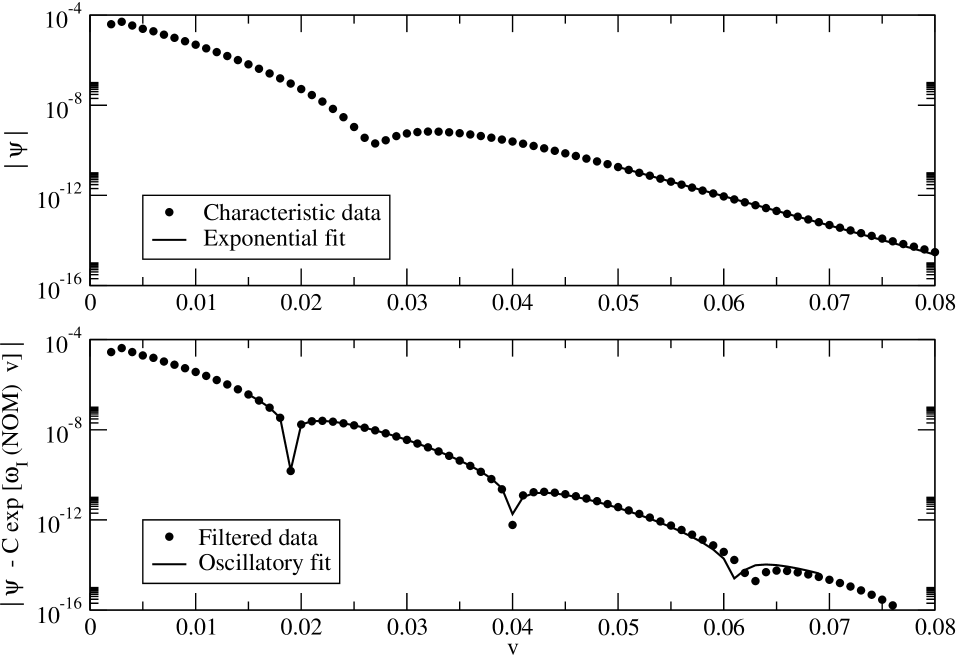
Figure 1: Illustration of the filtering process. (top) Data obtained from the characteristic algorithm. (bottom) The $\chi^{2}$-fitting made in the characteristic data subtracted from the Horowitz-Hubeny NOM solution. The results obtained from this fitting are compatible with the Horowitz-Hubeny OM results. In the graphs $r_{+}=100$, $Q/Q_{max}=0.41$, $R=1$, $\ell=0$ and $n=0$.

III Numerical results

III.1 Overview of the numerical results

Employing the Horowitz-Hubeny method to the high precision, we obtained two stable classes of solutions for the perturbation frequencies. In the first class, oscillation modes (OM) solutions, the frequencies have both the real and imaginary parts: $\omega(OM)=\omega_{R}(OM)+i\omega_{I}(OM)$, with $\omega_{R}(OM)\neq 0$. In the second class of solutions, the nonoscillation modes (NOM) solutions, the frequencies are purely imaginary: $\omega(NOM)=i\omega_{I}(NOM)$. In both cases, the imaginary part of the frequency is always negative, which indicates that the solutions are stable.

This scenario is consistent with the results obtained with time evolution approach. From the results obtained from the characteristic integration routine, it is possible to estimate with high precision the oscillatory and exponential decay parameters using a nonlinear fitting based in a $\chi^{2}$ analysis. Comparing to the results obtained by using the time evolution approach, we found that modes with frequencies choosing by $\min\left\{\sqrt{\omega_{R}(OM)^{2}+\omega_{I}(OM)^{2}},\sqrt{\omega_{I}(NOM)^{2}}\right\}$ is consistent with the results obtained by time evolution approach. We emphasize that the numerical concordance is excellent. Comparing to the time evolution approach can help us find the criterion to determine which class of solutions got by Horowitz-Hubeny method dominates the decay of the scalar field. We will use this criterion to order the modes.

On the other hand, no matter the criterion used to order the modes, both classes of solutions are physically relevant. The characteristic solutions of the wave equation show the asymptotic behavior of the field propagation. We observe two distinct “phases” with the increase of the electric charge. For small $Q$, the scalar field decays exponentially and oscillates. The frequencies in this case are compatible with the OM Horowitz-Hubeny solutions. For $Q$ greater than some critical value $Q_{c}$, the decay is purely exponential. The exponential coefficients are compatible with the NOM-Horowitz-Hubeny solutions.

But, even for large $Q/Q_{max}$, the characteristic approach does not exclude the OM solutions. It just says that the NOM solution dominates for large $t$. This does not invalidate the OM solution, because $\left|\omega_{I}(NOM)\right|<\left|\omega_{I}(OM)\right|$ and the oscillatory solutions could be present in the data, but hidden by the nonoscillatory solutions.

To expose the OM solution in the characteristic data, we will apply a filtering procedure: take the wave-function $\Psi(v)$ obtained from the characteristic integration; subtract from it the exponential part ($\omega_{I}(NOM)$) obtained from Horowitz-Hubeny method:

$$\Psi(v)\longrightarrow\Psi(v)-C\exp\left[\omega_{I}(NOM)\,v\right]\,\,;$$ (17)

and finally check if the remaining part is an oscillatory-exponential decaying function, compatible with the OM solutions.

Our results show that both modes are present in the characteristic results, although for large values of charge, the NOM solutions dominate the asymptotic limit, as indicated in Table 1. An illustration of the $\chi^{2}$-fittings made is shown in Fig. 1. To simplify notation, we will avoid the “$(OM)$” and “$(NOM)$”, except where it is not clear from the context.

Table 1: Values for the real and imaginary frequencies for the fundamental mode ($n=0$), obtained from Horowitz-Hubeny method (OM solutions) and filtered characteristic data, for $r_{+}=100$, $R=1$, $\ell=0$.

	Horowitz-Hubeny (OM solutions)		Frequencies after filtering
$Q/Q_{max}$	$\omega_{R}(OM)$	$\omega_{I}(OM)$	$\omega_{R}$ (error)	$\omega_{I}$ (error)
0.39	140.74	-340.47	138.27 (1.75%)	-328.98 (3.38%)
0.40	144.54	-344.62	146.96 (1.67%)	-355.71( 3.22%)
0.41	147.96	-347.49	148.78 ( 0.55%)	-347.52 ( 0.009%)
0.42	150.77	-349.57	151.10 ( 0.22%)	-348.96 ( 0.17%)
0.43	152.97	-351.20	153.71 ( 0.48%)	-350.88 ( 0.09%)
0.44	154.61	-352.59	156.02 ( 0.90%)	-352.70 ( 0.03%)

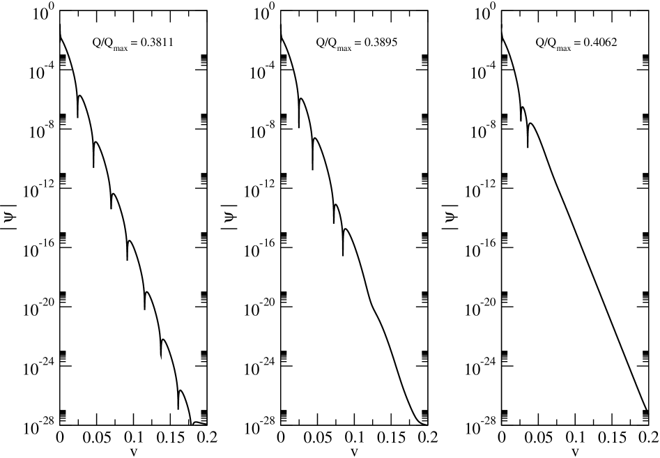
Figure 2: Semilog graphs of the scalar field in the event horizon, showing the transition from oscillatory to nonoscillatory asymptotic decay. In the graphs, $r_{+}=100$, $\ell=0$ and $R=1$.

As far as we have observed, the qualitative aspects of the field decay are independent of the value of the event horizon $r_{+}$. For completeness, we present in Table 2 some nonoscillatory frequencies for other values of $r_{+}$.

Table 2: Values for the nonoscillatory frequencies $\omega_{I}(NOM)$ for several values of $r_{+}$ and $\ell=0$, $Q/Q_{max}=0.35$, $R=1$.

$r_{+}$	$\omega_{I}(n=0)$	$\omega_{I}(n=1)$	$\omega_{I}(n=2)$	$\omega_{I}(n=3)$	$\omega_{I}(n=4)$	$\omega_{I}(n=5)$
90	-229.46	-663.64	-1105.3	-1547.9	-1990.7	-2433.5
100	-437.11	-1290.6	-2155.5	-3020.5	-3885.5	-4750.2
110	-805.32	-2448.5	-4093.9	-5738.2	-7381.9	-9025.3
120	-1486.7	-4562.5	-7632.0	-10698.5	-13763.5	-16827.8

III.2 Fundamental modes

III.2.1 Black holes with small values of charge

For the black holes with small values of the charge, it was found that $\omega_{I}$ increases with $Q$, while $\omega_{R}$ decreases with $Q$ Wang-00 ; Wang-01 . The change of the imaginary part of the frequency was supported, while the real part of the frequency was found not to have monotonically decreasing behavior Berti-03 . We have two complementary methods and expect to produce a more precise picture of the field’s evolution.

For black holes with small values of charge, the scalar field decays exponentially and oscillates. For $Q$ greater than a critical value, the decay becomes purely exponential. This point can be directly seen in the wave function plotting from Fig.2. We read from Fig.2 that the oscillation starts to disappear at $Q_{c}=0.3895Q_{max}$ (the first several rings in the plot $Q_{c}=0.3895Q_{max}$ are due to initial pulse).

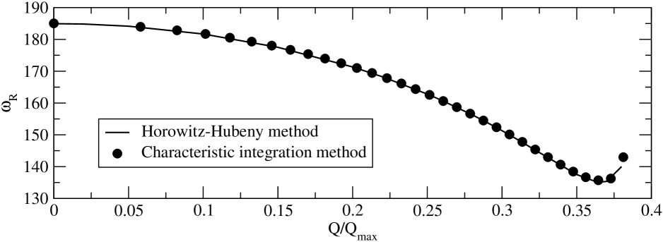
Figure 3: Graph of $\omega_{R}(OM)$ with $Q/Q_{max}$, using Horowitz-Hubeny method and characteristic integration results. For this graph, $r_{+}=100$, $R=1$, $\ell=0$ and $n=0$.

For $Q<Q_{c}$ the scalar perturbation experiences oscillation. The behavior of the real part of QN frequencies with the increase of the charge is shown in Fig.3, where results obtained from Horowitz-Hubeny and characteristic integration methods are presented.

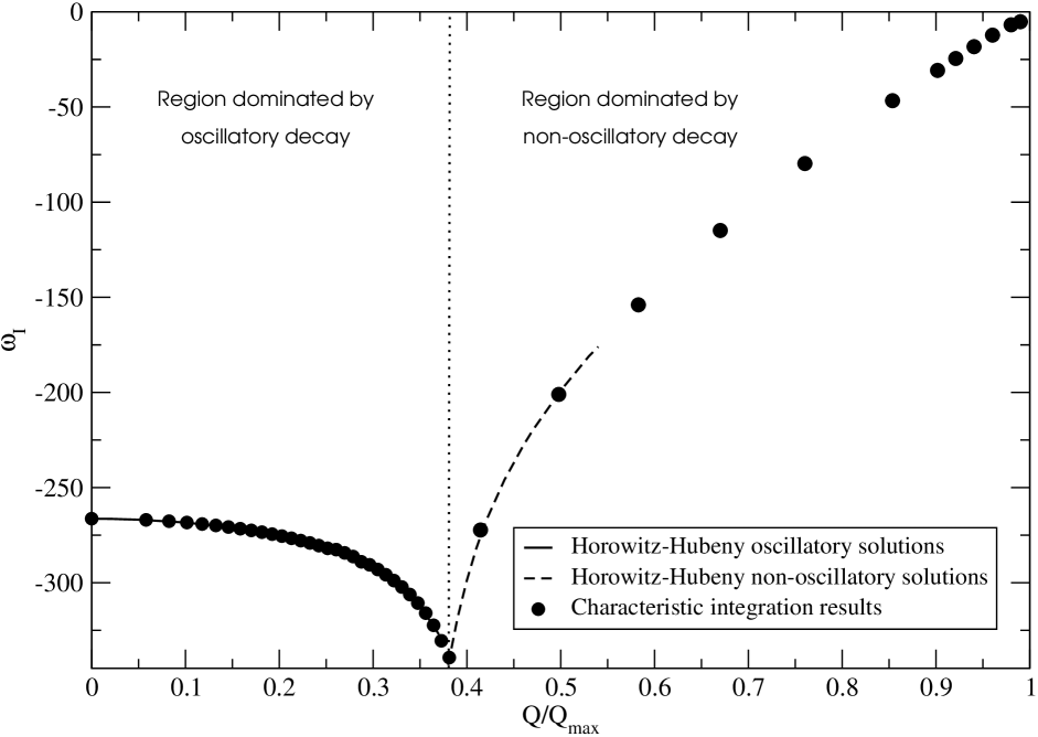
Figure 4: Graph of $\omega_{I}$ (OM and NOM) with $Q/Q_{max}$, showing that $\omega_{I}(NOM)$ tends to zero as $Q$ tends to $Q_{max}$. In the graph, $r_{+}=100$, $R=1$, $\ell=0$ and $n=0$.

It is apparent that the different numerical methods have very good agreement. We found indeed the minimum of $\omega_{R}$ at a certain value of charge, $Q_{e}=0.366Q_{max}$ from the Horowitz-Hubeny method and $Q_{e}=0.3645Q_{max}$ from the characteristic method. This result confirms that observed in Berti-03 . After the minima of $\omega_{R}$, $\omega_{R}$ increases with $Q$ a bit, but not as much as described in Berti-03 . Starting from $Q_{c}$, the NOM starts to dominate. The real part of the frequency of the perturbation vanishes and will not reach a local maxima at $Q=0.474Q_{max}$ as obtained in Berti-03 .

Now let us turn to discuss the imaginary part of the QN frequencies. Our two numerical methods give consistent results. From Fig.4, we found before $Q_{e}$ where $\omega_{R}$ has minima, $|\omega_{I}|$ monotonically increases with charge. This result agrees to that obtained in Wang-00 ; Berti-03 . However, there is no change of sign of the second derivative of $\omega_{I}(Q/Q_{max})$ as observed in Berti-03 . $|\omega_{I}|$ reaches its maxima at the same value of the charge $Q_{e}$ as $\omega_{R}$ arrives at its minima. For $Q<Q_{e}$, our previous statement is still valid, “If we perturb a RNAdS black hole with high charge, the surrounding geometry will not ‘ring’ as much and long as that of the black hole with small charge.” Wang-00 ; Wang-01 . For $Q>Q_{e}$, Fig.4 tells us that $|\omega_{I}|$ decreases with the increase of charge until $Q=Q_{max}$. The turning point of $\omega_{I}$ appears at a value of $Q$ that is not very big, and it is different from the rough argument in Wang-01 .

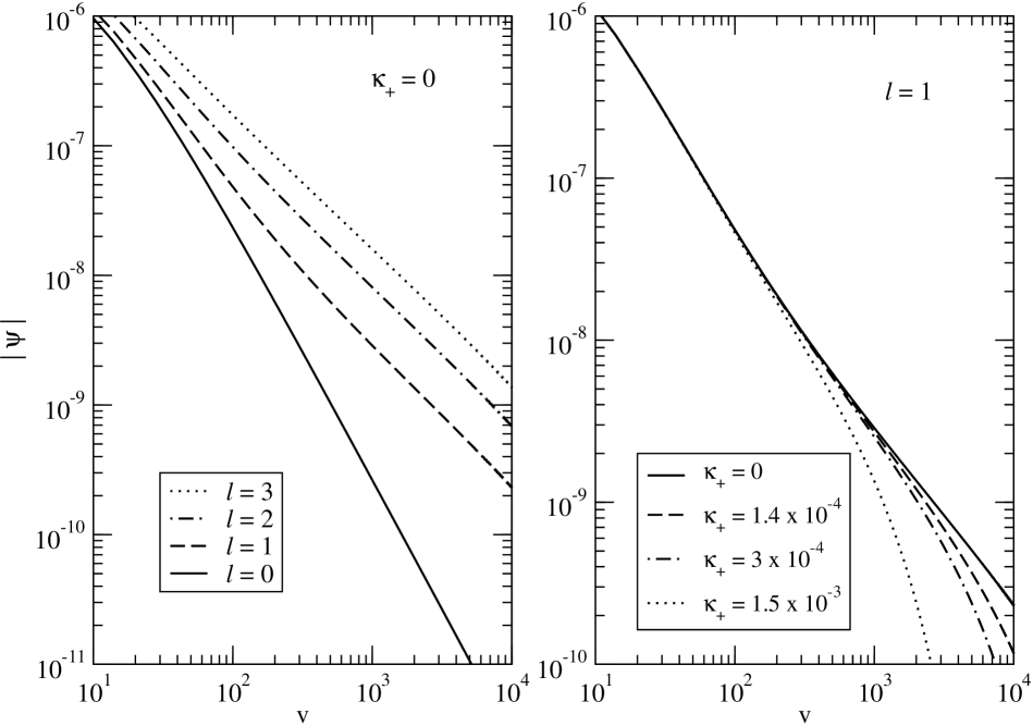
Figure 5: Log-log graphs of the scalar field in the event horizon. (left) Extreme case for different values of $\ell$, showing power-law tails. If $\ell=0$, $\Psi\propto v^{-2}$, but if $\ell>0$, $\Psi\propto v^{-1}$. (right) Approach to the extreme limit, showing transition from exponential decay to power-law decay ($\ell=1$). For all curves, $r_{+}=100$ and $R=1$.

III.2.2 Extreme and near extreme limits

From Fig.3 and Fig.4 we got the picture that for $Q>Q_{c}$ the asymptotic scalar perturbation is dominated by the nonoscillatory modes, while $|\omega_{I}|$ keeps decreasing monotonically and smoothly up to $Q=Q_{max}$. We learned from Fig.4 that as the black hole becomes extreme, $\omega_{I}$ tends to zero, which seems to confirm the conjecture raised in Section 3.3.2 of Berti-03 .

However, from the tail behavior (Fig.5) we observed that in the extreme limit, the decay of scalar perturbation still exists, though changing from the exponential to power-law decay. This result strongly suggests that due to scalar perturbations the extreme RNAdS black hole is stable, not marginally unstable as worried in Berti-03 by considering electromagnetic and axial gravitational perturbations.

The reason of the smooth change of the perturbation behavior can be understood as follows. In the extreme limit, the horizon $r_{+}$ is a double root of $h(r)$, and therefore the expression for the tortoise coordinate is given by

$$r_{ext}^{*}(r)=2A_{ext}\ln\left(r-r_{+}\right)-\frac{C}{r-r_{+}}-A_{ext}\ln(r^{2}+p_{ext}r\\ +q_{ext})+\frac{2(B_{ext}+Ap_{ext})}{\sqrt{4q_{ext}-p_{ext}^{2}}}\left[\arctan\left(\frac{2r+p_{ext}}{\sqrt{4q_{ext}-p_{ext}^{2}}}\right)-\frac{\pi}{2}\right]\\$$ (18)

with the constants $A_{ext}$, $B_{ext}$, $C$, $p_{ext}$ and $q_{ext}$ defined as

$$A_{ext}=\frac{R^{2}r_{+}\left(4r_{+}^{2}+R^{2}\right)}{\left(6r_{+}^{2}+R^{2}\right)^{2}}\,\,,$$ (19)

$$B_{ext}=\frac{R^{2}(6r_{+}^{4}+5r_{+}^{2}R^{2}+R^{4})}{\left(6r_{+}^{2}+R^{2}\right)^{2}}\,\,,$$ (20)

$$C=\frac{R^{2}r_{+}^{2}}{6r_{+}^{2}+R^{2}}\,\,,$$ (21)

$$p_{ext}=2r_{+}\,\,,\,\,q_{ext}=R^{2}+3r_{+}^{2}\,\,.$$ (22)

Globally, the structure of the extreme space-time changes drastically from that of the nonextreme Wang_Abdalla_Su . However, we will argue that, restricted to the exterior of the black hole, the transition from near extreme to extreme is, in a sense, smooth. To parametrize the approach to the extreme limit, we introduce the dimensionless variable

$$\delta=\frac{r_{+}-r_{-}}{r_{+}}\,\,.$$ (23)

In terms of $\delta$, the near extreme limit is given by $0<\delta\ll 1$, and the extreme case is $\delta=0$.

Let us analyze the two first terms in the expression for the tortoise function Eq.(4). We will expand these expressions in $\delta$. For this, we note that

$$\frac{1}{2\kappa_{+}}\ln\left(r-r_{+}\right)-\frac{1}{2\kappa_{-}}\ln\left(r-r_{-}\right)=-\left[\frac{1}{\delta}\frac{R^{2}r_{+}}{6r_{+}^{2}+R^{2}}-\frac{2R^{2}r_{+}\left(2r_{+}^{2}+R^{2}\right)}{\left(6r_{+}^{2}+R^{2}\right)^{2}}\right]\ln\left(1+\frac{r_{+}}{r-r_{+}}\delta\right)+O\left(\delta\right)\,\,.$$ (24)

At this point, it is necessary to consider another limit. If $r$ is not too close to the horizon, or more precisely, if $r_{+}\delta\ll r-r_{+}$ then

$$\frac{1}{2\kappa_{+}}\ln\left(r-r_{+}\right)-\frac{1}{2\kappa_{-}}\ln\left(r-r_{-}\right)=\frac{2R^{2}r_{+}\left(4r_{+}^{2}+R^{2}\right)}{\left(6r_{+}^{2}+R^{2}\right)^{2}}\ln\left(r-r_{+}\right)-\left(\frac{R^{2}r_{+}^{2}}{6r_{+}^{2}+R^{2}}\right)\frac{1}{r-r_{+}}+O\left(\delta\right)$$ (25)

On the other hand, for $r$ sufficiently close to $r_{+}$, or more specifically if $r_{+}\delta\gg r-r_{+}$:

$$\frac{1}{2\kappa_{+}}\ln\left(r-r_{+}\right)-\frac{1}{2\kappa_{-}}\ln\left(r-r_{-}\right)\approx\frac{1}{\delta}\frac{R^{2}r_{+}}{6r_{+}^{2}+R^{2}}\ln\left(r-r_{+}\right)$$ (26)

The near extreme approximations for the other terms in the tortoise functions are simpler, one can substitute $A\rightarrow A_{ext}$, $B\rightarrow B_{ext}$, $p\rightarrow p_{ext}$ and $q\rightarrow q_{ext}$, with an error of the order of $\delta$. Using the previous results, we find that in the near extreme limit we have

$$r^{*}(r)=\left\{\begin{array}[]{ccc}r^{*}_{ext}(r)+O\left(\delta\right)&\textrm{if}&\frac{r_{+}}{r-r_{+}}\delta\ll 1\\ \frac{1}{\delta}\frac{R^{2}r_{+}}{6r_{+}^{2}+R^{2}}\ln\left(r-r_{+}\right)+\cdots&\textrm{if}&\frac{r_{+}}{r-r_{+}}\delta\gg 1\end{array}\right.\,\,.$$ (27)

We see that for a certain value of $r$, the tortoise function becomes dominated by the power-law term, characteristic of the extreme function. When very near the horizon, the function $r^{*}(r)$ is dominated by a logarithmic term, which diverges when $r\rightarrow r_{+}$.

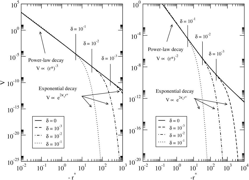
Figure 6: Log-log graphs of the function $V(r^{*})$, from the near extreme limit approaching the extreme limit. At a certain point, if $\delta>0$, there is a transition from power-law decay to exponential decay, indicated for each graph. For the curves, $r_{+}=100$, $R=1$ and $\ell=0,1$ (left and right figures, respectively).

For the effective scalar potential, using the previous results, we find that, if $r_{+}\delta\ll r-r_{+}$ , including the extreme limit where $\delta=0$:

$$V(r^{*})\propto\left\{\begin{array}[]{ccc}(r^{*})^{-2}&\textrm{if}&\ell>0\\ (r^{*})^{-3}&\textrm{if}&\ell=0\end{array}\right.\,\,.$$ (28)

The difference between $\ell=0$ and $\ell>0$ in expression (28) comes from the presence of a non-null term $\ell(\ell+1)/r^{2}$ in the potential. This is reflected in the asymptotic behavior of the wave functions, as seen in Fig.5(left).

If $\delta>0$, the behavior of the effective potential can be different if the observation point is sufficiently close to the event horizon. More precisely, if $r-r_{+}\ll\delta r_{+}$, the exponential decay dominates, and

$$V(r^{*})\propto e^{2\kappa_{+}r^{*}}\,\,.$$ (29)

The different potential asymptotic forms, when $Q$ is close to $Q_{max}$, depend on whether we are initially near to the black hole horizon or not. This difference will disappear in the black hole extreme limit ($\delta\rightarrow 0$) as illustrated in Fig.6. As $\delta$ approaches zero, the potential is more and more dominated by the power-law phase, and the exponential tail is less relevant. In the extreme limit, there is only a power-law tail. This smooth change in the RNAdS potential explains the smooth change in the wave functions from the near extreme to extreme limit, illustrated in Fig.5(right).

III.3 Higher modes

The first numerical study of the high overtone QN frequencies for scalar perturbation was done in SAdS black hole Cardoso_Lemos . We have extended their investigation to RNAdS spacetimes and found that “switching on the charge” brings interesting physics. For the higher modes, the time evolution method is not practical. However the Horowitz-Hubeny method is still efficient, at least for values of the charge not too big.

For the same value of the charge, both real and imaginary part of QN frequencies increases with the overtone number $n$. This result confirms that observed in Cardoso_Lemos .

There are large variations of both $\omega_{R}$ and $\omega_{I}$ with the charge and the overtone number. Figure 7 tells us that with the increase of $Q$, $\omega_{R}$ increases slower while $|\omega_{I}|$ increases faster for bigger overtone number $n$.

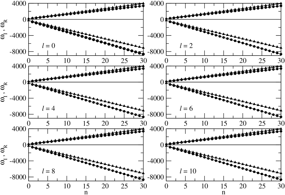
Figure 7: Graphs of $\omega_{R}(OM)$ and $\omega_{I}(OM)$ versus $n$, for $Q/Q_{max}=0.1$ (represented by triangles) and $Q/Q_{max}=0.4$ (represented by bullets). The continuous lines indicate the linear fits. With the increase of Q, $\omega_{R}(OM)$ increases slower with $n$, while $|\omega_{I}(OM)|$ increases faster with $n$. For the curves, $r_{+}=100$, $R=1$ and $\ell=0,2,4,6,8,10$.

For $\omega_{R}$, combining Fig.3 and Fig.8, we see that the local minima of the “wiggle” appear at smaller values of the charge with the increase of $n$. The “wiggle” of $\omega_{R}$ becomes shallower with the increase of $n$ and disappears for $n\geq 5$ as exhibited in Fig.8. Further with the increase of $n$, we observed that $\omega_{R}$ starts to be zero at bigger values of charge. For the imaginary part of the QN frequencies, the relation with $n$ and $Q$ are shown in Figs.9 and 10. We found that with the increase of $n$, the maxima of $|\omega_{I}|$ appear at bigger values of black hole charge. Moreover we saw from Fig.10 that before the maxima, $|\omega_{I}|$ increases quicker with charge for bigger $n$. These richer physics are brought by introducing the additional parameter $Q$ in RNAdS spacetimes.

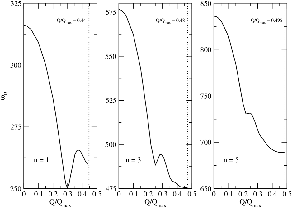
Figure 8: Graphs of $\omega_{R}(OM)$ with $Q/Q_{max}$, showing the “wiggle behavior”. Values of $Q/Q_{max}$ in graphs indicating when nonoscillating solution dominates. For the curves, $r_{+}=100$ and $\ell=0$.

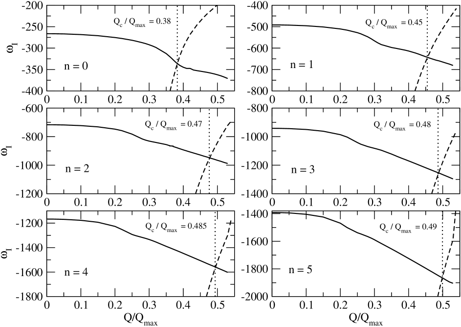
Figure 9: Graphs of $\omega_{I}$ (OM and NOM solutions) with $Q/Q_{max}$ for several values of $n$. The continuous lines indicate the oscillatory solution, dotted lines indicate nonoscillatory solutions. For the curves, $r_{+}=100$, $R=1$ and $\ell=0$.

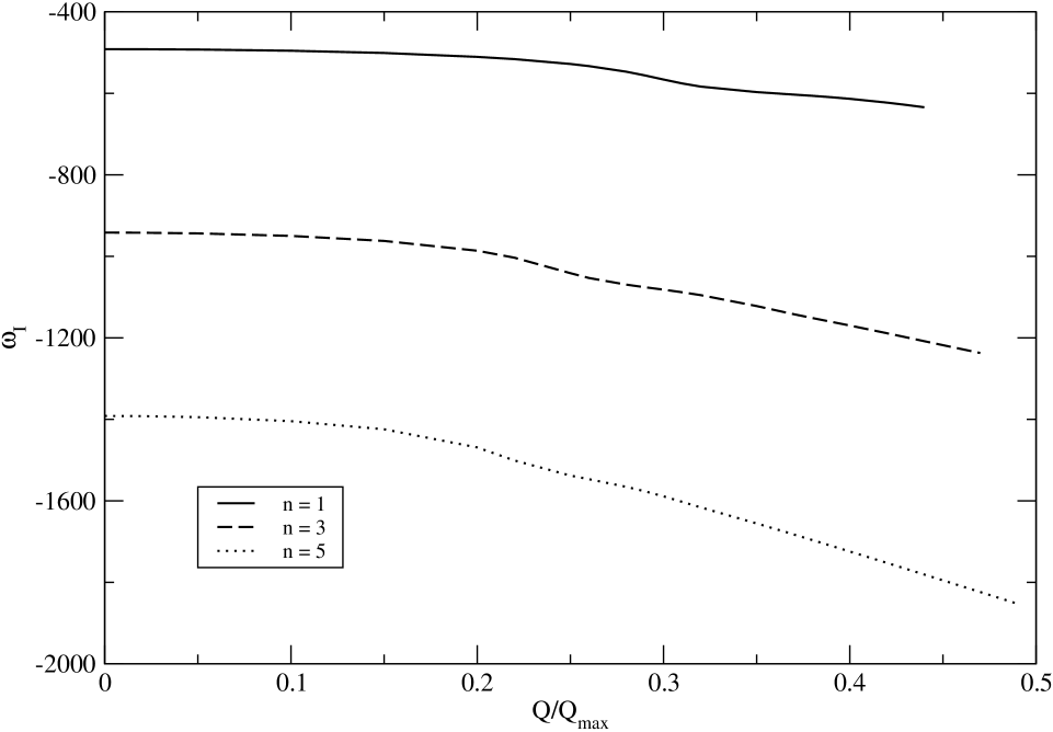
Figure 10: Graphs of $\omega_{I}(OM)$ with $Q/Q_{max}$, showing the increase of $|\rm{Im}(\omega)|$ with $n$. For the curves, $r_{+}=100$, $R=1$, $\ell=0$ and $n=0$.

In Cardoso_Konoplya_Lemos it was interestingly found that in the large black hole regime the frequencies become evenly spaced for high overtone number $n$. For lowly charged RNAdS black hole, our result confirmed their argument for fixed value of the charge. The spacing between frequencies are

$$\omega_{n+1}-\omega_{n}=129.9-225i,\hskip 28.45274pt(n\rightarrow\infty\,\,\textrm{when}\,\,Q=0),$$ (30)

which is the same as (12) in Cardoso_Konoplya_Lemos by choosing $r_{+}=100$ there, and

$$\omega_{n+1}-\omega_{n}=120.6-233i$$

$$(n\rightarrow\infty\,\,\textrm{when}\,\,Q=0.15Q_{max}),$$ (31)

$$\omega_{n+1}-\omega_{n}=111.1-256i,$$

$$(n\rightarrow\infty\,\,\textrm{when}\,\,Q=0.3Q_{max}).$$ (32)

We found that choosing bigger values of the charge, the real part in the spacing expression becomes smaller, while the imaginary part becomes bigger.

III.4 Dependence on the angular index $\ell$

We have so far discussed only the QNMs with $\ell=0$. Increasing $\ell$, for the lowest lying mode, we obtained the effect of decreasing of $\omega_{I}$ and increasing of $\omega_{R}$ in RNAdS spacetimes Wang-00 ; Wang-01 , though the dependence is very weak Berti-03 . In studying the higher modes, it was argued that the asymptotic behavior of the spacing of high overtones is independent of the value of $\ell$ Cardoso_Konoplya_Lemos .

Our numerical computations show that although QNM frequencies depend very weakly on $\ell$, the dependence is not trivial. As was found in the lowest lying mode, $\omega_{R}$ increases and $|\omega_{I}|$ decreases with the increase of $\ell$. Besides, a quadratic adjustment fits very well the dependence of the modes will $\ell$, as seen in Fig.11-14. This property holds independently of the values of charge and the overtone number we calculated. However we observed that $\omega_{R}$ increases and $|\omega_{I}|$ decreases slower with $\ell$ when $n$ increases.

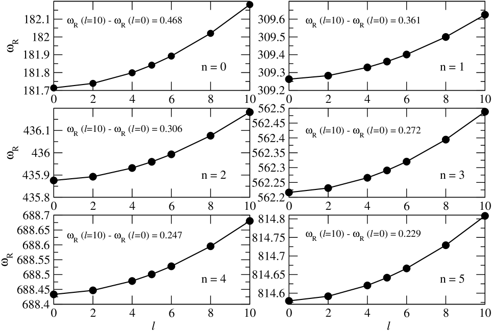
Figure 11: Graphs of $\omega_{R}(OM)$ with $\ell$, for several values of $n$. The bullets indicate the numerical results and the lines indicate the quadratic fittings. For the curves, $r_{+}=100$, $R=1$ and $Q/Q_{max}=0.1$.

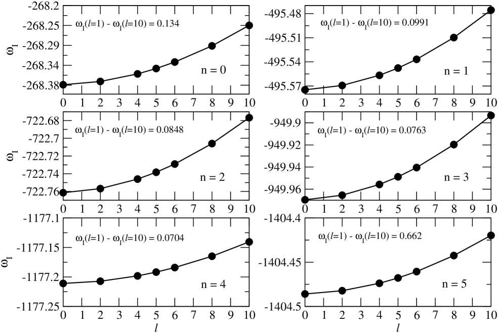
Figure 12: Graphs of $\omega_{I}(OM)$ with $\ell$, for several values of $n$. The bullets indicate the numerical results and the lines indicate the quadratic fittings. For the curves, $r_{+}=100$, $R=1$ and $Q/Q_{max}=0.1$.

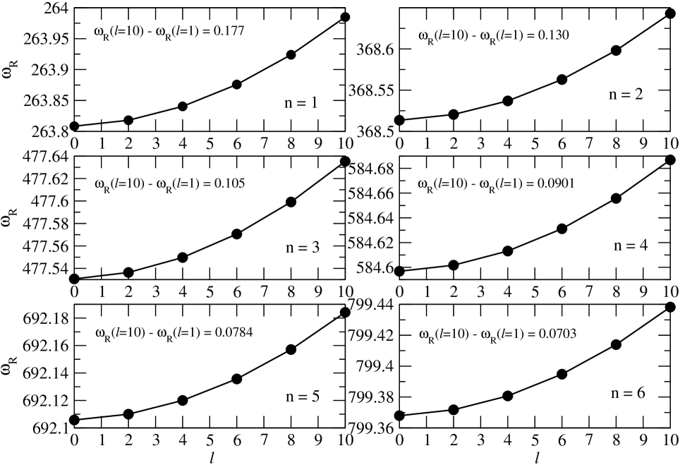
Figure 13: Graphs of $\omega_{R}(OM)$ with $\ell$, for several values of $n$. The bullets indicate the numerical results and the lines indicate the quadratic fittings. For the curves, $r_{+}=100$, $R=1$ and $Q/Q_{max}=0.4$.

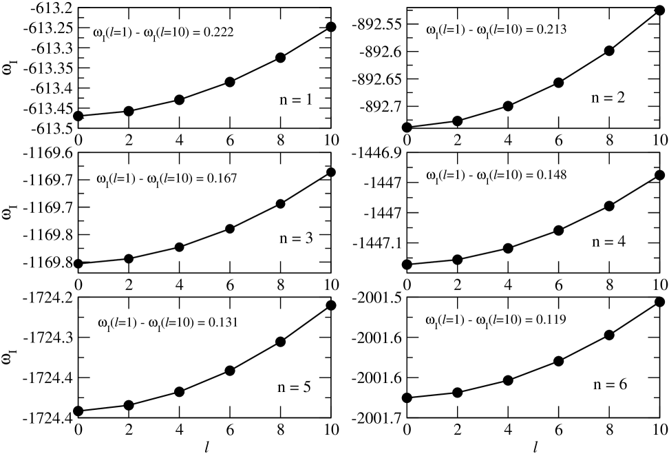
Figure 14: Graphs of $\omega_{I}(OM)$ with $\ell$, for several values of $n$. The bullets indicate the numerical results and the lines indicate the quadratic fittings. For the curves, $r_{+}=100$, $R=1$ and $Q/Q_{max}=0.4$.

IV Conclusions and discussions

We have presented a comprehensive study of scalar perturbations of a Reissner-Nordström anti-de Sitter spacetime, and computed its quasinormal modes. We observed the presence of two families of solutions, both physically relevant. For $Q$ smaller than a critical value, the asymptotic decay is dominated by oscillating modes, while for larger values of $Q$, the decay is dominated by purely exponential modes. Similar situation was observed in the Reissner-Nordström de Sitter (RNdS) geometry, where $\Lambda$ was the critical parameter [4].

For the lowest lying QNMs, our results verify (or sometimes disprove) and extend many results obtained in Horowitz-00 ; Wang-00 ; Wang-01 ; Cardoso ; Berti-03 . The real part of the QN frequency does have a local minimum at $Q/Q_{max}=0.366$, however when $Q>0.3895Q_{max}$, the NOM starts to dominate. For this class of quasinormal modes, the real part of frequency vanishes. When selecting the mode class (OM or NOM) which dominates the decay, we found that the imaginary part of the QN frequency $|\omega_{I}|$ has maxima at the same values of charge where $\omega_{R}$ has minima. Before these maxima, $|\omega_{I}|$ increases monotonically with charge (OM solution), while after that $|\omega_{I}|$ keeps on decreasing until the black hole extreme limit (NOM solution). We observed that under the scalar perturbation the imaginary part of the frequency tends to zero, as previously conjectured in the electromagnetic and axial gravitational perturbations Berti-03 . In the extreme limit, the asymptotic field decay is dominated by a power-law tail, which suggests that this geometry is stable to scalar perturbations. A similar field behavior was observed in the RNdS case deSitter_2 in the approach to $\Lambda=0$ limit.

We have done an extensive search for higher overtones $n$ of the QNMs of RNAdS black hole corresponding to scalar perturbations. We have observed large variations of QN frequencies with the overtone number and black hole charge. Both real and imaginary parts of QN frequencies are evenly spaced for high overtone number $n$ at fixed $Q$. The spacings between frequencies varies with the black hole charge. The nontrivial quadratic dependence of QN frequencies on angular index $\ell$ has also been addressed.

- (1) H. P. Nollert, Class. Quant. Grav. 16, R159 (1999).
- (2) K. D. Kokkotas and B. G. Schmidt, Living Rev. Rel. 2, 2 (1999).
- (3) P. R. Brady, C. M. Chambers, W. Krivan and P. Laguna, Phys. Rev. D 55, 7538 (1997); P. R. Brady, C. M. Chambers, W. G. Laarakkers and E. Poisson, Phys. Rev. D 60, 064003 (1999); T.Roy Choudhury, T. Padmanabhan, Phys. Rev. D 69 064033 (2004); D. P. Du, B. Wang and R. K. Su, hep-th/0404047.
- (4) C. Molina, Phys.Rev. D 68 064007 (2003); C. Molina, D. Giugno, E. Abdalla, A. Saa, Phys.Rev. D 69 104013 (2004).
- (5) J. S. F. Chan and R. B. Mann, Phys. Rev. D 55, 7546 (1997); J.S.F. Chan and R.B. Mann, Phys. Rev. D 59, 064025 (1999).
- (6) G. T. Horowitz and V. E. Hubeny, Phys. Rev. D 62, 024027 (2000).
- (7) B. Wang, C.Y. Lin, and E. Abdalla, Phys. Lett. B 481, 79 (2000).
- (8) B. Wang, C. Molina, and E. Abdalla, Phys. Rev. D 63, 084001 (2001).
- (9) V. Cardoso and J.P.S. Lemos, Phys. Rev. D 63, 124015 (2001); V. Cardoso and J.P.S. Lemos, Phys. Rev. D 64, 084017 (2001); V. Cardoso and J.P.S. Lemos, Class. Quantum Grav. 18, 5257 (2001).
- (10) E. Berti and K.D. Kokkotas, Phys. Rev. D 67, 064020 (2003).
- (11) R. A. Konoplya, Phys. Rev. D 66, 044009 (2002).
- (12) D. Birmingham, I. Sachs, S. N. Solodukhin, Phys. Rev. Lett. 88, 151301 (2002); D. Birmingham, Phys.Rev. D 64, 064024 (2001).
- (13) J.M. Zhu, B. Wang, and E. Abdalla, Phys. Rev. D 63, 124004 (2001); B. Wang, E. Abdalla and R. B. Mann, Phys. Rev. D 65, 084006 (2002).
- (14) S. Musiri, G. Siopsis, Phys. Lett. B 576, 309-313 (2003); R. Aros, C. Martinez, R. Troncoso, J. Zanelli, Phys. Rev. D 67, 044014 (2003); A. Nunez, A. O. Starinets, Phys.Rev. D 67,124013 (2003); E. Winstanley, Phys. Rev. D 64, 104010 (2001); V. Cardoso, J. Natario and R. Schiappa, hep-th/0403132; R.A. Konoplya, Phys.Rev.D 66, 084007 (2002).
- (15) V. Cardoso and J. P. S. Lemos, Phys. Rev. D 67, 084020 (2003).
- (16) V. Cardoso, R. Konoplya and J. P. S. Lemos, Phys. Rev. D 68, 044024 (2003).
- (17) I. G. Moss and J. P. Norman, Class. Quant. Grav. 19, 2323 (2002).
- (18) C. Gundlach, R. Price and J. Pullin, Phys. Rev. D 49, 883 (1994).
- (19) B. Wang, E. Abdalla and R. K. Su, Phys. Rev. D 62, 047501 (2000).