PROSPECTS FROM STRINGS AND BRANES

A brief, non-technical and non-exhaustive review of D(irichlet)-branes and (some) of their applications is given.

1 Introduction

In this paper I will give a brief account of string theory with particular emphasis on D-branes and their applications. A more extensive account can be found in a paper by Augusto Sagnotti and the author which also provides a more comprehensive list of references.$\!{}^{{\bf?}}$ Because of the very nature of this contribution, I will mainly cite review papers or books.$\!{}^{{\bf?}}$ Further references to the original literature can be found in there.

Einstein’s general relativity gives a remarkably good classical description of the gravitational interaction. However, any naive attempt to quantize general relativity fails as the theory is non-renormalizable. This means that the elimination of ultra-violet divergences – endemic to quantum field theories – necessitates the introduction of an infinite number of parameters, all to be determined by experiments. This is clearly not an acceptable situation. Modifying the ultra-violet structure of the theory by smearing out the interactions cures this problem. In casu, we replace point particles by tiny strings as shown on figure 1.

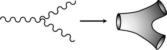
Figure 1: By replacing point particles with strings, a graviton three-point interaction e.g (left) is “smeared” such that in the resulting three-string vertex (right) no localized interaction point can be found anymore.

String theory is not new. In fact it finds its roots in the late sixties, early seventies, as an attempt to describe the strong interaction. However, in that context it encountered a grave problem: in the particle spectrum of a string theory one always finds a massless spin 2 particle. With the advent of QCD, string theory was abandoned as a theory of the strong force but it lived on as a candidate for a theory of quantum gravity (the graviton is a massless spin 2 particle).

The supersymmetric version of string theory is ultra-violet finite. It contains both the gravitational and the other interactions in such a way that in the infra-red regime they effectively reduce to (a supersymmetric extension of) general relativity and gauge theories. While this looks very encouraging, one has to face the problem that consistency of string theory at the quantum level requires it to live in 9 space-like dimensions and 1 time-like dimension. In other words: the theory only exists in 10 (or $9+1$) dimensions. This obvious problem can be solved in two ways (or a combination of these):

• Make the superfluous dimensions very small. This is known as compactification. Compare this to a garden hose which, from far away, looks like a one-dimensional object. The precise shape and volume of the compact dimensions determines to a large extent the physics in the four uncompactified dimensions. This immediately leads to another problem. While string theory puts very severe consistency requirements on the compact space, numerous solutions are known. A physical principle to select the “right one” is still lacking.

• Make the extra dimensions very dark. This covers to a large extent the brane-world scenarios. The main idea is that the gauge interactions are confined to our four-dimensional world while the gravitational interaction propagates in the full ten-dimensional space. This option is reviewed in more detail in the contribution of Lisa Randall in this volume.

As mentioned, string theory allows for a very large number of different ways to realize either one or a combination of those options. The quest for a selection mechanism requires insight in the non-perturbative properties of string theory. This is a highly non-trivial task as a string theory is essentially defined as a set of self-consistent Feynman rules and as consequence it is purely perturbative. With the discovery of D-branes in 1995, certain non-perturbative issues became addressable.

2 D-branes

Strings occur in two versions: closed and open strings. Roughly speaking, one has that closed strings carry the gravitational interaction and the open strings carry the gauge interactions. While closed strings can freely propagate in space, the modern point of view is that the end points of open strings are “stuck” on $p$-dimensional hypersurfaces, where $p\in\{1,2,\cdots,9\}$. These hypersurfaces are known as Dp-branes. They are dynamical but they are extremely heavy in the perturbative regime of string theory (their tension or energy per unit of volume is inversely proportional to the string coupling constant): they are solitons. A D0-brane is a point-like object, a D1-brane a string-like object, a D2-brane a membrane, … Just as a propagating point particle sweeps out a curve – the world-line – in space-time, a Dp-brane sweeps out a $p+1$-dimensional volume – the world-volume – in the 10-dimensional space-time. The effective dynamics on the world-volume is then described by a $p+1$-dimensional field theory.

What are the degrees of freedom in this field theory? Looking at a single Dp-brane, one finds that the bosonic degrees of freedom are a $U(1)$ gauge field (a photon) and $9-p$ scalar fields together with their fermionic partners. Both types of fields arise from the fluctuations of the open strings ending on the brane. The photon corresponds to fluctuations longitudinal to the brane while the scalar fields are associated to the fluctuations of the string transversal to the brane. In the infra-red, the effective field theory on the brane is simply a supersymmetric version of Maxwell theory coupled to $9-p$ scalar fields.

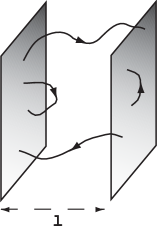
Figure 2: Open (oriented) strings can attach themselves in four different ways to two parallel D-branes. The mass of the gauge field associated to each of these open strings is proportional to the shortest distance between the branes they connect. Whenever $l\neq 0$, one has two massless gauge fields, with a corresponding unbroken $U(1)\times U(1)$ symmetry, and two additional massive $W$-like fields. On the other hand, when $l\rightarrow 0$ the two $W$-like fields become massless as well, and the gauge symmetry is enhanced to $U(2)$. This yields a geometric setting for the Brout-Englert-Higgs mechanism. The Higgs scalar describes the fluctuations of the branes relative to one another with its vacuum expectation value corresponding to the relative distance, $l$, between the branes.

Once more D-branes are present, the situation becomes interesting. The mass of an open string is proportional to the shortest distance between the two branes it connects. As explained in figure 2, when several, say $n$ branes coincide, additional massles gauge fields appear and the gauge symmetry grows from $(U(1))^{n}$ to $U(n)$.

3 Applications

3.1 (Non-)abelian gauge theories and their solutions

The effective field theory describing $n$ D-branes is in leading order a supersymmetric gauge theory with gauge group $U(n)$. In this way, D-branes provide an excellent laboratory to study various aspects and solutions of gauge theories in a very geometric setting. The Brout-Englert-Higgs mechanism, discussed in the previous section, provided a first example.

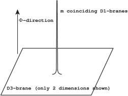
Figure 3: The Dirac magnetic monopole with flux $m$ is realized in string theory as a D3-brane with $m$ D1-branes perpendicular to it.

Another simple and instructive example is Dirac’s magnetic monopole.$\!{}^{{\bf?}}$ Consider (in 3 dimensions) an electro-magnetic potential of the form,

$$A_{x}^{(\pm)}=-\frac{m}{2}\frac{y}{r(z\pm r)},\quad A_{y}^{(\pm)}=+\frac{m}{2}\frac{x}{r(z\pm r)},\quad A_{z}^{(\pm)}=0,$$ (1)

where $r\equiv\sqrt{x^{2}+y^{2}+z^{2}}$ and $A^{(+)}$ ($A^{(-)}$ resp.) is defined for $\theta>-\varepsilon$ ($\theta<\varepsilon$ resp.), with $\theta$ the azimuthal angle and $\varepsilon>0$ and small. If one requires that on the overlap of the two patches ($-\varepsilon<\theta<\varepsilon$), $A^{(+)}$ and $A^{(-)}$ are related by a single valued gauge transformation, one obtains the celebrated Dirac quantization condition: $m\in\mathbb{Z}$. The magnetic field $\vec{B}=\nabla\times\vec{A}$, satisfies,

$$\nabla\cdot\vec{B}=2\pi m\,\delta(\vec{x}),$$ (2)

thus signalling the presence of a magnetic monopole at the origin.

In the language of D-branes, one realizes this as follows. One starts with a single D3-brane stretched in the $x-y-z$ directions, together with a scalar field $\Phi$ which has the background value, $\Phi=m/2r$. The field equations are satisfied if the magnetic field is given by $\vec{B}=-\nabla\Phi$ which is precisely Dirac’s monopole field. As explained before, a scalar field corresponds to a direction perpendicular to the D3-brane. A careful analysis of the various charges shows that this is a stable D-brane configuration consisting of a single D3-brane with $m$ D1-branes perpendicular to it thereby giving yet another interpretation/derivation of Dirac’s quantization condition. The system is illustrated in figure 3.

In fact, to the authors knowledge, almost all monopole and instanton configurations find a natural realization in terms of D-branes. This setting provides not only a classification of such solutions but elucidates many of their properties (e.g. the ADHM construction of instanton solutions) as well. In fact, only one class of gauge configurations escaped a D-brane interpretation: the octonionic monopoles in 7 and the octonionic instantons in 8 dimensions. However, even these solutions might very well find their place in a D-brane context.$\!{}^{{\bf?}}$

3.2 Black Holes

A spectacular application of strings and branes occurs in the study of black holes.$\!{}^{{\bf?}}$ A static, isotropic object of mass $M$ with a radius $R$, smaller than the Schwarzschild radius $R_{s}=2G_{N}Mc^{-2}$ ($G_{N}$ is Newton’s constant) is a (Schwarzschild) black hole. The (imaginary) sphere with radius $R_{S}$ around the black hole is called the event horizon. Physics inside the event horizon is completely disconnected from physics outside it. Taking quantum mechanics into account, Hawking showed that black holes are not really black but that they radiate thermally with temperature,

$$T_{H}\ =\ \frac{c^{3}\,\hbar}{8\pi k_{B}G_{N}M}\ ,$$ (3)

where $k_{B}$ denotes Boltzmann’s constant. Using the second law of thermodynamics, one finds the entropy $S_{H}$,

$$\frac{1}{k_{B}}\;S_{H}\ =\ \frac{4\pi G_{N}M^{2}}{c\hbar}\ =\ \frac{1}{4}A_{H}\,\ell_{Pl}^{-2}\ ,$$ (4)

where $A_{H}$ is the area of the horizon in Planck units and $\ell_{Pl}$ is the Planck length $\ell_{Pl}=\sqrt{G_{N}\hbar/c^{3}}\approx\ 10^{-33}\,cm$. The fact that the entropy is 1/4 of the surface of the horizon in Planck units is a universal behavior of all black holes. Furthermore, as was shown by ’t Hooft, a black hole is the physical system which maximizes the entropy in a given volume. These simple observations raise three profound questions.

1. The entropy of a black hole is characterized by a few macroscopic quantities. In our example there is only the mass $M$, the more general case can have some charges, angular momentum, … Since Boltzmann, we know that entropy measures the degeneracy of microstates in some underlying microscopic description of the system. Since the entropy (4) of a black hole is an unusually large number, how can one realize such a wealth of microstates?

2. Any object coming from outside and crossing the horizon is trapped inside it forever, leaving only thermal radiation behind. A black hole is a very simple object: no matter how diversified the objects absorbed by it, the result is characterized by a few macroscopic quantities. This seems to imply that the S-matrix of a system containing a black hole seems not unitary anymore, thus violating one of the basic axioms of quantum mechanics (the information paradox).

3. As a black hole maximizes the entropy within a given volume, it is highly unusual that the entropy is proportional to the surface of the horizon rather than to its volume. This led ’t Hooft and Susskind to the holographic principle: any theory with gravity (and as a consequence with black holes) in a given volume should somehow be equivalent to a theory without gravity (hence without black holes) living on the boundary of the volume. While both attractive and spectacular, one would like to have concrete realizations of the holographic principle.

For a certain class of black holes, the extremal and near-extremal black holes, the first two questions were solved. Starting from the effective field theory describing the infra-red regime of a certain string theory (a specific supersymmetric extension of general relativity) one looks for black hole solutions characterized by their energy and some charges. Performing Hawking’s program yields then an expression for the entropy. Subsequently one constructs within the corresponding string theory stable D-brane configurations wrapped around the compact dimensions with open strings ending on them which give rise to the same energy and charges. Usually their are numerous configurations giving rise to the same macroscopic numbers and it is quite spectacular that the resulting degeneracy exactly reproduces the macroscopically calculated entropy.

For a near-extremal black hole the radiation of the system can be studied as well. Hawking radiation turns out, as shown in figure 4, to arise from the annihilation of open strings resulting in an open string remaining on the brane and a closed string leaving the brane. This radiation is exactly thermal with both temperature and radiation in perfect agreement with Hawking’s calculation. By construction this approach is unitary and the apparently lost information appears to reside in the D-branes.

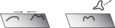
Figure 4: The D-brane picture of Hawking radiation. A pair of open strings collide, giving rise to a closed string that leaves the brane. As a result, Hawking radiation reaches the bulk via the emission of closed strings.

3.3 Holography and the AdS/CFT correspondence

The third problem cited in the previous section – holography – can as well be addressed in the context of D-branes.$\!{}^{{\bf?}}$ Maldacena considered a stack of $m$ D3-branes in IIB string theory in flat space. Taking the low energy limit in a specific way one finds that the bulk physics (containing a non-interacting version of gravity) decouples from the brane physics (a $U(m)$ $N=4$ supersymmetric Yang-Mills theory in $3+1$ dimensions ). Alternatively, looking at IIB supergravity (the effective field theory describing the infra-red regime of IIB superstrings) one constructs a solution having the same quantum numbers as the stack of D3-branes. The decoupling limit turns out in this case to be the near-horizon limit which has the topology of $AdS_{5}\times S^{5}$, with $S^{5}$ the 5-dimensional sphere and $AdS_{5}$ 5-dimensional anti-de Sitter space. For our purposes, it is sufficient to know that the latter is a manifold with a negative cosmological constant which has 4-dimensional Minkowski space as its boundary. The previous observations led Maldacena to the conjecture that string theory on $AdS_{5}\times S^{5}$ is equivalent or dual to $U(m)$ $N=4$ supersymmetric Yang-Mills theory living on the boundary, i.e. $3+1$ dimensional Minkowski space. The concrete mapping between observables at both sides of this duality were found thereby providing a first concrete example of holography. While this is still a conjecture, it passed numerous tests and checks. The map between both theories is quite remarkable as the supergravity description of string theory (a purely classical limit) corresponds to the strongly coupled limit of the corresponding $U(m)$ gauge theory. In other words, classical calculations in supergravity yield non-perturbative information on a gauge theory. Since this seminal examples, many other instances of holography were found and the gravity/gauge map has become a powerful tool to study previously inaccessible features of gauge theories (e.g. Dijkgraaf and Vafa mapped the full non-perturbative holomorphic sector of $N=1$ supersymmetric gauge theories to a classical matrix model).

3.4 Cosmology

Observational evidence strongly points to the fact that the expansion of our universe is presently in an accelerating phase.$\!{}^{{\bf?}}$ Let us first look at some elementary issues.$\!{}^{{\bf?}}$ Approximating the universe by a perfect fluid (characterized by an energy density $\rho$ and a pressure $p$), one finds that it is described by the Robertson-Walker line element,

$$d\tau^{2}=dt^{2}-R(t)^{2}\left(dr^{2}+r^{2}d\theta^{2}+r^{2}\sin^{2}\theta d\phi^{2}\right),$$ (5)

where we assumed a flat topology for space (as is favored by the data). The scale factor $R(t)$ is determined by the Einstein equations which reduce to,

$$\dot{R}^{2}=\frac{8\pi G_{N}}{3}R^{2}\left(\rho+\frac{\lambda}{8\pi G_{N}}\right),$$

$$\dot{\rho}+(\rho+p)\frac{3\dot{R}}{R}=0.$$ (6)

with $\lambda$ the cosmological constant. In order to solve these equations, one needs an equation of state, i.e. a relation between the pressure $p$ and the energy density $\rho$. The simplest ansatz is a constant linear relation,

$$p(t)=\alpha\,\rho(t) \Rightarrow \rho=\rho_{0}\frac{R_{0}^{3(\alpha+1)}}{R^{3(\alpha+1)}},$$ (7)

with $\alpha\in\mathbb{R}$. The subindex $0$ denotes the present value of the corresponding quantities. For non-relativistic dust one has $\alpha=0$, radiation gives $\alpha=1/3$ and a positive cosmological constant corresponds to $\alpha=-1$. Using eq. (7) in eq. (6) yields,

$$\alpha\neq-1 R(t)\propto t^{2/3(\alpha+1)},$$

$$\alpha=-1 R(t)\propto e^{\sqrt{\lambda}t/\sqrt{3}}.$$ (8)

Note that a positive cosmological constant ($\alpha=-1$) gives rise to an exponentially growing expansion, also known as inflation. From eq. (6) we immediately derive an expression for the change in the expansion rate,

$$\frac{\ddot{R}}{R}=-\frac{4\pi G}{3}(1+3\alpha)\rho+\frac{\lambda}{3}.$$ (9)

One notices that a positive cosmological constant ($\lambda>0$) results in acceleration. So does any “matter” (meaning that $\rho>0$) which satisfies the equation of state, eq. (7) with $\alpha<-1/3$. Present data favors $-1.62<\alpha<-0.74$. Models with $\alpha<-1$ describe so-called phantom matter which will not further be discussed here . If the acceleration is caused by a positive cosmological constant ($\alpha=-1$), one has to face the cosmological constant problem. Indeed, the observed vacuum energy density associated to it is of the order $\rho_{vac}\sim\left(10^{-3}\,eV\right)^{4}$. If one compares this to the Planck scale, $(10^{19}GeV)^{4}$, one finds an ${\cal O}(10^{124})$ mismatch! Comparison with the supersymmetry breaking breaking scale, $(10^{3}GeV)^{4}$, improves the situation but still leaves an ${\cal O}(10^{60})$ discrepancy! In fact it turns out to be very hard to accommodate for a very small but non-zero cosmological constant. Because of this, the anthropic principle currently undergoes a revival…

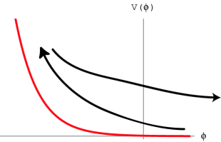
Figure 5: A typical potential of the form $V\propto e^{-2a\phi}$. Initially the field starts from the right with a large negative velocity. It rolls up the hill, looses kinetic energy and enters a transitional accelerating epoch. During this period the constants of nature vary extremely slowly.

Turning to string theory, the situation even worsens. In 10- or 11-dimensional supergravity (the supersymmetric extensions of general relativity which describe the infra-red regime of string theory), the second derivative of the scale factor is directly related to the Ricci tensor, $\ddot{R}(t)=-R_{00}=-4\pi(T_{00}+g^{ij}T_{ij})$ with $T$ the energy-momentum tensor and $g$ the metric. Both 10- and 11-dimensional supergravity satisfy the strong energy condition, $R_{00}>0$, and as a consequence can never accommodate an accelerating universe. Gibbons and later Nuñez and Maldacena studied 11- and 10-dimensional supergravity compactified to four dimensions on a static 7- or 6-dimensional space with metric,

$$ds^{2}_{11,10}=\omega^{2}(y)ds_{4}^{2}(x)+ds_{7,6}^{2}(y),$$ (10)

where $y$ collectively denote the compact coordinates. A straightforward calculation shows then that $R^{(11,10)}_{00}\geq 0\Rightarrow R_{00}^{(4)}\geq 0$. In other words, this looks as if string theory can never accommodate for an accelerating universe. There are two ways out. Ultra-violet effects might modify the behavior of the theory in such a way that acceleration does become possible. As the full ultra-violet behavior of string theory is not known yet, we leave this possibility for what it is. The other way is to reassess the premises of the no-go theorem. Doing so one immediately notices the word static.

Before delving deeper, let me mention that the shape, volume, … of the compact space in string theory is steered by scalar fields (which generically are ubiquitous in string theory). Consider the simple case of a single, uniform scalar field $\phi$ with a potential $V(\phi)$, living in a Robertson-Walker background. Its equation of motion is given by,

$$\ddot{\phi}=-V(\phi)^{\prime}-3H\dot{\phi},\qquad H\equiv\dot{R}/R,$$ (11)

where the dot denotes a time derivative and a prime a derivative with respect to $\phi$. The Robertson-Walker background provides a time-dependent friction term. The energy density and pressure for this system are given by,

$$\rho=\frac{1}{2}\dot{\phi}{}^{2}+V(\phi),\qquad p=\frac{1}{2}\dot{\phi}{}^{2}-V(\phi).$$ (12)

One notices that if both the kinetic energy is sufficiently small and the potential $V(\phi)$ is positive, acceleration occurs. The previously stated no-go theorem required a static compactification, in other words $\phi$ is time independent. So from the equation of motion (11) one sees that the no-go theorem implies that the potential has no stationary points with $V>0$. Allowing non-static compactifications yields a way around the no-go theorem.

A typical situation in string theory $\!{}^{{\bf?}}$ – arising both in flux and in hyperbolic compactifications – is a potential $V(\phi)=b\,e^{-2\,a\,\phi},$ with $b>0$. For hyperbolic compactifications one has $1\,<\,a\,<\,\sqrt{3}$, while for flux compactifications $a>\sqrt{3}$ holds. At a far past, $\dot{\phi}\ll 0$ and $\phi\gg 0$. As shown in figure 5, when time evolves, the field rolls up the hill while $\dot{\phi}$ approaches zero. Around the turning point we get a transient accelerating phase (during which the constants of nature, determined by the moduli fields are nearly constant). While this might be an explanation for the current acceleration, one could wonder whether this scenario might also explain the initial inflation in the early universe. A detailed investigation shows that it cannot as the number of e-foldings is far less than what is required to solve the horizon and flatness problems. More subtle models which include orientifold planes and branes and which cannot so easily be captured in a supergravity language can actually reproduce intitial inflation.$\!{}^{{\bf?}}$ $\!{}^{{\bf?}}$

3.5 Particle physics

From the very beginning of string theory as a quantum theory of gravity, serious efforts were invested in the study of its consequences for particle physics phenomenology. Before the advent of D-branes, the efforts were concentrated on model building starting from the heterotic string string. Now that we have D-branes, new possibilities open up, some of which are reviewed elsewhere in this volume.

We already mentioned the flux compactifications.$\!{}^{{\bf?}}$ In these models the moduli are fixed by turning on fluxes for certain generalized gauge configurations (essentially for the so-called Ramond-Ramond fieldstrengths). This approach which has many interesting applications (see e.g. the previous subsection) has the drawback that the generation of chiral fermions is very hard. More involved model building along these lines is in full development.

Another intriguing development are the so-called intersecting brane worlds.$\!{}^{{\bf?}}$ In these, various stacks of branes are considered (the strong, the weak and the electro-magnetic) which have a 3-dimensional intersection - our world - where all three forces are simultaneously present. It turns out that it is easy to generate the Standard Model gauge group, 3 families of quarks and leptons, … Unfortunately, there are many ways to achieve this. Generic features of these models are the presence of right-handed neutrinos and two or more Higgs scalars. An important difficulty is the issue of stability. (In order for this to work the branes have to intersect in a very specific way, however the branes tend to recombine.) Furthermore, the status of the hierarchy problem – at least for toroidal and orbifold compactifications – is unclear. Finally – and related to the stability issue – the construction of an intersecting brane world which yields the MSSM was till recently an open problem. However, very recently there was serious progress towards solving this problem.$\!{}^{{\bf?}}$ At present a lot of effort is dedicated towards the construction of the low-energy effective action and the identification of the generic “beyond-the-Standard-Model” features of these models.

4 Conclusions

From the previous, it is clear that string theory accounts for several successes. Indeed, both the microscopic understanding of (a class of) black holes and the realization of holography are highlights. The close relation of D-branes with gauge theories provides a novel way of studying various aspects of gauge theories from a geometric perspective. However, from a purely particle physicists point of view, one has to admit that concrete qualitative, let alone quantitative post- or predictions are not yet in sight. While both flux compactifications and intersecting brane worlds are very valuable ideas which are thoroughly being explored, a mechanism for selecting the “right” vacuum is not yet available.

In the absence of this, one has recently started to explore an alternative way to arrive at predictions, which is the study of the so-called string theory landscape.$\!{}^{{\bf?}}$ In this statistical approach one counts the number of vacua having more or less the same physical properties, i.e. having the same values for certain fundamental parameters. (Because of e.g. hidden sectors, there might be a very large number of different vacua yielding all similar four dimensional physics.) One would expect that the most probable value for these parameters are those which are realized by the largest number of vacua. While this approach is still in its infancy – only relatively simple classes of models have already been investigated – the first results are not really encouraging: neither low energy supersymmetry breaking nor large extra dimensions are favored. But then again, it will take another year or two of research along these lines before hard statements can be made.

Finally, very recent ideas where the possibility of very large relic strings in the cosmos might lead to concrete predictions testable in gravitational wave detectors such as LIGO. $\!{}^{{\bf?}}$

References

References

- [1] A. Sagnotti and A. Sevrin, in the proceedings of the XXXVIII Rencontres de Moriond on Electroweak Interactions and Unified Theories, (2002), hep-ex/0209011
- [2] A popular book on string theory was written by B.R. Greene, The Elegant Universe, W.W. Norton & Co, 1999. Two interesting and easily accessible texts are, J. Polchinski, String duality: A colloquium, Rev. Mod. Phys. 68 (1996) 1245, hep-th/9607050 and M. J. Duff, M theory (the theory formerly known as strings), Int. J. Mod. Phys. A 11, 5623 (1996), hep-th/9608117. The two “standard” books on string theory are, M. B. Green, J. H. Schwarz and E. Witten, Superstring Theory, 2 vols., Cambridge Univ. Pr., 1987 and J. Polchinski, String Theory, 2 vols., Cambridge Univ. Pr., 1998. A more technical and very extensive review on D-branes is, C. V. Johnson, D-brane primer, hep-th/0007170.
- [3] G. W. Gibbons, Branes as BIons, Class. Quant. Grav. 16 (1999) 1471, hep-th/9803203.
- [4] A. Keurentjes, P. Koerber, A. Sevrin and A. Wijns, in preparation.
- [5] C. Callan, Black holes in string theories: some surprising new developments, in “Les Arcs 1997, Electroweak interactions and unified theories”, 185; T. Damour, The entropy of black holes: A primer, hep-th/0401160.
- [6] E. Witten, New perspectives in the quest for unification, hep-ph/9812208; O. Aharony, S. S. Gubser, J. M. Maldacena, H. Ooguri and Y. Oz, Large N field theories, string theory and gravity, Phys. Rept. 323 (2000) 183 hep-th/9905111; R. Bousso, The holographic principle, arXiv:hep-th/0203101; L. Thorlacius, Black holes and the holographic principle, hep-th/0404098.
- [7] D. N. Spergel et al., First Year Wilkinson Microwave Anisotropy Probe (WMAP) Observations: Determination of Cosmological Parameters, Astrophys. J. Suppl. 148 (2003) 175, astro-ph/0302209, S. M. Carroll, Why is the universe accelerating?, eConf C0307282 (2003) TTH09, astro-ph/0310342.
- [8] M. Trodden and S. M. Carroll, TASI lectures: Introduction to cosmology, astro-ph/0401547.
- [9] S. M. Carroll, M. Hoffman and M. Trodden, Can the dark energy equation-of-state parameter w be less than -1?, Phys. Rev. D 68 (2003) 023509, astro-ph/0301273; G. W. Gibbons, Phantom matter and the cosmological constant, hep-th/0302199.
- [10] P. K. Townsend and M. N. R. Wohlfarth, Accelerating cosmologies from compactification, Phys. Rev. Lett. 91 (2003) 061302 hep-th/0303097; R. Emparan and J. Garriga, A note on accelerating cosmologies from compactifications and S-branes, JHEP 0305 (2003) 028 hep-th/0304124; P. K. Townsend, Cosmic acceleration and M-theory, hep-th/0308149.
- [11] S. Kachru, R. Kallosh, A. Linde and S. P. Trivedi, De Sitter vacua in string theory, Phys. Rev. D 68 (2003) 046005, hep-th/0301240; S. Kachru, R. Kallosh, A. Linde, J. Maldacena, L. McAllister and S. P. Trivedi, Towards inflation in string theory, JCAP 0310 (2003) 013, hep-th/0308055.
- [12] E. Silverstein, TASI / PiTP / ISS lectures on moduli and microphysics, hep-th/0405068.
- [13] D. Lüst, Intersecting brane worlds: A path to the standard model?, Class. Quant. Grav. 21 (2004) S1399, hep-th/0401156.
- [14] G. Honecker and T. Ott, Getting just the supersymmetric standard model at intersecting branes on the Z(6)-orientifold, hep-th/0404055; C. Kokorelis, N=1 Supersymmetric Standard Models with No Massless Exotics from Intersecting Branes, hep-th/0406258.
- [15] F. Denef and M. R. Douglas, Distributions of flux vacua, JHEP 0405 (2004) 072, arXiv:hep-th/0404116.
- [16] E. J. Copeland, R. C. Myers and J. Polchinski, Cosmic F- and D-strings, JHEP 0406 (2004) 013, hep-th/0312067.