Collision of Domain Walls and Reheating of the Brane Universe

Abstract

We study a particle production at the collision of two domain walls in 5-dimensional Minkowski spacetime. This may provide the reheating mechanism of an ekpyrotic (or cyclic) brane universe, in which two BPS branes collide and evolve into a hot big bang universe. We evaluate a production rate of particles confined to the domain wall. The energy density of created particles is given as $\rho\approx 20\bar{g}^{4}N_{b}~{}m_{\eta}^{4}$ where $\bar{g}$ is a coupling constant of particles to a domain-wall scalar field, $N_{b}$ is the number of bounces at the collision and $m_{\eta}$ is a fundamental mass scale of the domain wall. It does not depend on the width $d$ of the domain wall, although the typical energy scale of created particles is given by $\omega\sim 1/d$. The reheating temperature is evaluated as $T_{\rm R}\approx 0.88~{}\bar{g}~{}N_{b}^{1/4}$. In order to have the baryogenesis at the electro-weak energy scale, the fundamental mass scale is constrained as $m_{\eta}\mbox{\raisebox{-4.30554pt}{$\stackrel{{\scriptstyle\textstyle>}}{{\textstyle\sim}}$}}1.1\times 10^{7}$ GeV for $\bar{g}\sim 10^{-5}$.

I introduction

The big bang theory is very successful because it naturally explains the evolution of our universe from the nucleosynthesis to the present time with many observational data. However, it contains some theoretical key problems such as the flatness and the horizon problems22 ; 21 . So far, only the idea of inflation provides a resolution of those problems. Not only it gives some picture of the earlier stage of the universe before a big bang but also it seems to be supported by some of recent observational data on CMB. While, it is still unclear what is the origin of inflaton. So far, there is no convincing link with fundamental unified theories such as a string/M theory.

Recently a new paradigm on the early universe has been proposed, which is so-called a brane world1 ; 3 . Such speculation has been inspired by recent developments in string/M-theoryWitten ; String ; Polchinski . There has been tremendous works in this scheme of dimensional reduction where ordinary matter fields are confined to a lower-dimensional hypersurface, while only gravitational fields propagate throughout all of spacetime. In particular, it was shown that the 10-dimensional $E_{8}\times E_{8}$ heterotic string theory, which is a strong candidate to describe our real world, is equivalent to an 11-dimensional M theory compactified to ${\bf M}^{10}\times{\bf S}^{1}/Z_{2}$ Witten . Then the 10-dimensional spacetime is expected to be compactified into ${\bf M}^{4}\times{\bf CY}^{6}$, where ${\bf M}^{4}$ and ${\bf CY}^{6}$ are 4-dimensional Minkowski spacetime and 6-dimensional Calabi-Yau space, respectively. Randall and Sundrum 4 also proposed a new model where four-dimensional Newtonian gravity is recovered at low energies even without compact extra dimensions. Based on such a new world picture, many cosmological scenario have been studied brane_cosmology ; brane_cosmo2 ; Lukas . See also recent reviewsMaeda ; Maartens ; Langlois ; Brax . We have found some deviations from standard cosmology by modifications of 4-dimensional Einstein equations on the braneshiromizu , even for the case there is a scalar field in bulkMaeda_Wands .

In such a brane world scenario, for resolving the above-mentioned theoretical key problems in the big bang theory, new idea of the early universe has been proposed, which is called the ekpyrotic scenario or a cyclic universe scenario Khoury ; Khoury_cyclic . It is based on a collision of two cold branes. The universe starts with a cold, empty and nearly BPS ground state of M theory, which contains two parallel branes at rest. Two branes approach each other and then collide. The energy is dissipated on the brane and the big bang universe will start. The BPS state is required in order to remain a supersymmetry in a low-energy 4-dimensional effective action. The visible and hidden branes are flat, which are described by a Minkowski spacetime, but the bulk is warped along the fifth dimension. Since this scenario is not only motivated by the fundamental unified theory but also it may resolve the theoretical key problems such as the flatness and horizon problems, it would be very attractive. There are also many discussions about density perturbations to see whether this scenario is really a reliable model for the early universedensity_ekpyrotic ; density_ekpyrotic2 ; density_ekpyrotic3 ; density_ekpyrotic4 .

On the other hand, even though there are some works bykofman , the reheating process itself in this scenario has not been so far investigated in detail. Hence, in this paper, we study how we can recover the hot big bang universe after the collision of the branes. Here we investigate quantum creation of particles, which are confined to the brane, at the collision of two branes. It may be difficult to deal properly with the collision of two branes in a basic string theory. Hence, in this paper, we adopt a domain wall which is constructed by some scalar field as a brane, and analyze the collision of two domain walls in a 5-dimensional bulk spacetime. Some works also adopt such a picture Copeland ; Dvali . It is worth noting that there is a thick domain wall model for a brane worldsakai .

In order to analyze particle creation at the brane collision, in this paper we consider the simplest situation. We discuss that two domain walls collide in a 5D Minkowski spacetime. In Sec. II, we analyze the collision of two domain walls. Then, in Sec. III, we investigate particle creation on the wall at the collision. Applying the particle production to the energy dissipation of the brane, we discuss the reheating mechanism of a brane universe. We use the unit of $c=\hbar=1$.

II collision of two domain walls

II.1 Basic equations and initial setting

We study the collision of two flat domain walls in 5-dimensional (5D) Minkowski spacetime. To construct a domain wall structure, we adopt a real scalar field $\Phi$ with a double-well potential,

$$V(\Phi)=\frac{\lambda}{4}(\Phi^{2}-\eta^{2})^{2}\,,$$ (1)

where the potential minima are located at $\Phi=\pm\eta$.

We discuss the collision of two parallel domain walls. The scalar field is assumed to depend only on a time coordinate $t$ and one spatial coordinate $y$. The rest three spatial coordinates are denoted by $x$. We rescale the parameters and variables by $\eta$ (or its mass scale $m_{\eta}=\eta^{2/3}$) as

$$\ \tilde{t}=m_{\eta}t\ ,\ \tilde{y}=m_{\eta}y\ ,\tilde{\Phi}=\frac{\Phi}{\eta}\ ,\ \tilde{\lambda}=m_{\eta}\lambda\ .$$ (2)

In what follows, we omit the tilde in dimensionless variables for brevity.

The equation of motion for $\Phi$ in 5D is given by

$$\ddot{\Phi}-\Phi^{\prime\prime}+\lambda\,\Phi\,(\Phi^{2}-1)=0\,,$$ (3)

where $\dot{}$ and ^′ denote ${\partial}/{\partial t}$ and ${\partial}/{\partial y}$, respectively.

Eq. (3) has not only two stable vacuum solutions $\Phi_{\pm}=\pm 1$ but also a static kink solution (${K}$), which is topologically stable. The latter one is called a domain wall, which is described by

$$\Phi_{K}(y)=\tanh\left[\ \frac{y}{d}\ \right]\quad,\$$ (4)

where $d=\sqrt{{2}/{\lambda}}$ is the thickness of the wall 11 . The antikink solution ($\bar{K}$) is obtained from Eq. (4) by reflecting the spatial coordinate $y$ as $\Phi_{\bar{K}}(y)=\Phi_{K}(-y)=-\Phi_{K}(y)$. A single domain wall solution moving with a constant speed $\upsilon$ in the $y$ direction is given by boosting the solution (4). We find a moving domain wall solution, whose initial position is located at $y=0$, as

$$\Phi_{\upsilon}(y,t)=\tanh\left[\ \frac{\gamma}{d}\left(y-\upsilon t\right)\ \right]\ ,$$ (5)

where $\gamma=1/\sqrt{1-\upsilon^{2}}$ is the Lorentz factor.

In order to discuss the collision of two domain walls, we first have to set up the initial data. We put a kink and an antikink solution, which are separated at large distance, and are moving toward each other with velocities $\upsilon$ and $-\upsilon$. The explicit initial configuration is given by

$$\Phi(y,0)=\Phi_{\upsilon}(y+y_{0},0)-\Phi_{-\upsilon}(y-y_{0},0)-1\ ,$$ (6)

where $y=\pm y_{0}$ is the initial position of the walls. The spatial separation of two walls is given by $2y_{0}$, and as long as the separation distance is much larger than the thickness of a wall ($y_{0}\gg d$), the initial profile (6) gives a good approximate solution for two moving domain walls. The initial value of $\dot{\Phi}$ is also given by

$$\dot{\Phi}(y,0)=\dot{\Phi}_{\upsilon}(y+y_{0},0)-\dot{\Phi}_{-\upsilon}(y-y_{0},0)\ .$$ (7)

Using this initial values, we solve the dynamical equation (3) numerically, whose results will be shown in the next subsection.

II.2 Time Evolution of Domain Walls

We use a numerical approach to solve the equations for the colliding domain walls. The numerical method is shown in Appendix A. We have two free parameters in our simulation of the two-wall collision, i.e. a thickness of the wall ${d}=\sqrt{2/{\lambda}}$ and an initial velocity of the walls ${\upsilon}$. The collision of two walls was discussed by fractal in 4-dimensional Minkowski space. Although we discuss the domain wall collision in 5-dimensional Minkowski space, our basic equations are exactly the same as their case, and then we find the same results as theirs. In particular, the results are very sensitive to the initial velocity $\upsilon$.

First we show the numerical results for two typical initial velocities, i.e. $\upsilon=0.2$ and 0.4 in Figs. 1, 2. The evolution of the energy density of $\Phi$ is shown in Figs. 1 and 2. The energy density of the scalar field is given by

$$\rho_{\Phi}=\frac{1}{2}\left[\dot{\Phi}^{2}+{\Phi^{\prime}}^{2}+\frac{\lambda}{2}(\Phi^{2}-1)^{2}\right]\,.$$ (8)

From Figs. 1 and 2, we find some peaks of the energy density, by which we can define the positions of moving walls ($y=\pm y_{\rm W}(t)$).

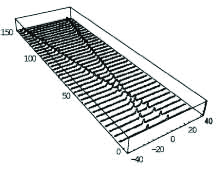
Figure 1: Collision of two domain walls for the case of the initial velocity $\upsilon=0.4$. The time evolution of the energy density of scalar field $\Phi$ is shown from $t=0$ to 150. The maximum point of $\rho_{\Phi}$ defines the position of a wall ($y=y_{\rm W}(t)$).

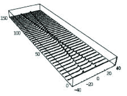
Figure 2: Collision of two domain walls for the case of the initial velocity $\upsilon=0.2$. The time evolution of the energy density of the scalar field $\Phi$ is shown from $t=0$ to 150. We find that collision occurs twice at $t\approx 58$ and 77. We set ${\lambda}=1.0$. From this figure, we find clearly that collision occurs twice.

From Figs. 1 and 2, we see the detail of the collision as follows. For the case of initial velocity $\upsilon=0.4$, we find that, the collision occurs once, while it does twice for the case of $\upsilon=0.2$. To be precise, in the latter case, after two walls collide first, they bounce, recede to a finite distance, and then return to collide again.

As shown by several authors fractal ; 13 ; 14 ; 15 , however, the result highly depends on the incident velocity $\upsilon$ . In Appendix B, we show our detail analysis, which confirms the previous works. For a sufficiently large velocity, it is expected that a kink and antikink will just bounce off once because there is no time to exchange the energy during the collisional process. In fact, it was shown in fractal that two walls just bounce off once for $\upsilon\mbox{\raisebox{-4.30554pt}{$\stackrel{{\scriptstyle\textstyle>}}{{\textstyle\sim}}$}}0.25$. For smaller velocity, we find multiple bounces when they collide. The number of bounce during the collision depends complicatedly on the incident velocity. For example, the bounce occurs once for $\upsilon=0.4$, while twice for $\upsilon=0.2$. We also find many bounce solutions for other incident velocities as shown in Appendix B (see also fractal ). We find that the number of bounce is not monotonic function of $\upsilon$, but is much more complicated. If we change the incident velocity slightly, the number of bounce changes. The existence of a fractal structure in the parameter space is shown in Fig. 6 of fractal .

III Particle production on a moving domain wall

III.1 Quantization of a particle on the domain wall and its production rate

Once we find the solution of colliding domain walls, we can evaluate the time evolution of a scalar field on the domain wall. Since we assume that we are living on one domain wall, we are interested in production of a particle confined to the domain wall. We assume that there is some coupling between a 5D scalar field $\Phi$ which is responsible for the domain wall and a particle on the domain wall. Because the value of the scalar field changes with time, we expect quantum particle production occurs. This may be important for a reheating mechanism of the colliding domain walls.

Hence we have to know the value of the scalar filed $\Phi$ on the domain wall, i.e. $\Phi_{\rm W}(\tau)=\Phi(t,y_{\rm W}(t))$. Since the wall is moving in a 5D Minkowski space, we have to use the proper time $\tau$ of the wall, which is given by

$$\tau=\int^{t}_{0}dt\sqrt{1-\dot{y}_{\rm W}^{~{}2}(t)}\,\,,$$ (9)

when we estimate the particle production in our 4-dimensional domain wall.

We consider a particle on the domain wall which is described by a scalar field $\psi$. We assume that it is confined to the domain wall and couples to the scalar field $\Phi$ as

$$g^{2}\,\phi^{2}(\tau)\psi^{2}\,,$$ (10)

where $g$ is a coupling constant. Here $\phi(\tau)$ is the 4-dimensional scalar field, which is induced from the 5-dimensional $\Phi$ as

$$\phi(\tau)\approx\sqrt{2d}~{}\Phi_{\rm W}(\tau)\ .$$ (11)

We have also assumed that the effective width of the domain wall when it collides is about $2d$, which is confirmed by numerical simulation. In Fig. 3, we depict the spatial distribution of the scalar field $\Phi$ when the domain walls collide. Note that $\Phi_{\rm w}(\tau)$ is the maximum amplitude in this distribution.

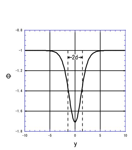
Figure 3: The spatial distribution of the scalar field $\Phi$ when the domain walls collide. $d$ is the thickness of the wall. The scalar field has non-vanishing value for the effective width of $2d$ at the collision.

The basic equation for $\psi$ is then

$$\frac{\partial^{2}\psi}{\partial\tau^{2}}-\nabla^{2}\psi+\bar{g}^{2}\,\Phi_{\rm W}^{2}(\tau)\,\psi=0\ ,$$ (12)

where

$$\bar{g}^{2}=2dg^{2}={2\sqrt{2}\over\lambda^{1/2}}\,g^{2}\ .$$ (13)

Since our background spacetime is the 4-dimensional Minkowski space, it is easy to quantize the scalar field $\psi$. In a canonical quantization scheme quantum , we expand $\psi$ as

$$\psi(\tau,\mbox{\boldmath$x$})=\sum_{k}[a_{k}\,\psi_{k}(\tau)\,u_{k}(\mbox{\boldmath$x$})+a_{k}^{{\dagger}}\psi_{k}^{*}(\tau)u_{k}^{*}(\mbox{\boldmath$x$})]\ ,$$ (14)

where $u_{k}(\mbox{\boldmath$x$})=(2\pi)^{-\frac{3}{2}}e^{i\mbox{\boldmath$k$}\cdot\mbox{\boldmath$x$}}$. The wave equation (12) for each mode is now

$$\ddot{\psi_{k}}+[k^{2}+\bar{g}^{2}\Phi_{\rm W}^{2}(\tau)]\psi_{k}=0\ ,$$ (15)

where $k=|\mbox{\boldmath$k$}|$. Since two domain walls are initially far away each other, the value of $\Phi_{\rm W}$ is almost zero. We can quantize $\psi$ as a usual quantization scheme. The eigen function with a positive frequency is given by

$$\psi_{k}^{({\rm in})}={1\over\sqrt{2\omega_{k}}}e^{-i\omega_{k}\tau}\ ,$$ (16)

where $\omega_{k}=\sqrt{k^{2}+\bar{g}^{2}\Phi_{\rm W}^{2}(0)}\approx k$. We impose the equal time commutation relation for the operators $a_{k}$ and $a_{k}^{{\dagger}}$

$$[a_{k},a_{k^{\prime}}]=0\ ,$$ (17)

$$[a_{k}^{{\dagger}},a_{k^{\prime}}^{{\dagger}}]=0\ ,$$ (18)

$$[a_{k},a_{k^{\prime}}^{{\dagger}}]=\delta_{kk^{\prime}}\ ,$$ (19)

where $a_{k}$ and $a_{k}^{{\dagger}}$ are an annihilation and a creation operators. We then define a vacuum $|0>_{\rm in}$ at $\tau=0$ by $a_{k}$ as

$$a_{k}|0>_{\rm in}=0\quad\ ,\ \forall k\ .$$ (20)

After the collision of domain walls, we expect that the value of $\Phi_{\rm W}$ again approaches zero (see the detail in the next subsection). We can also define the vacuum state $|0>_{\rm out}$, which is different from the initial vacuum state $|0>_{\rm in}$. The eigen function of $\psi_{k}$ for $\tau\rightarrow\infty$ is then given by a linear combination of $\psi_{k}^{({\rm in})}$ and $\psi_{k}^{({\rm in})*}$ as

$$\psi_{k}^{({\rm out})}=\alpha_{k}\,\psi_{k}^{({\rm in})}+\beta_{k}\,\psi_{k}^{({\rm in})*}\ ,$$ (21)

and the annihilation and creation operators as

$$\bar{a}_{k}=\alpha_{k}a_{k}+\beta_{k}^{*}a_{k}^{{\dagger}}\ ,$$ (22)

where $\alpha_{k},\ \beta_{k}$ are the Bogolubov coefficients, which satisfy the normalization condition

$$|\alpha_{k}|^{2}-|\beta_{k}|^{2}=1\ .$$ (23)

The Hamiltonian of this system is given by

$$:H: = -\int_{\tau={\rm const}}:T^{0}_{~{}~{}0}:\,d^{3}\mbox{\boldmath$x$}$$ (24)

$$= \sum_{k}a_{k}^{{\dagger}}a_{k}\omega_{k}\ ,$$

where : : is the normal ordering operation. The creation of the particles with mode $k$ is evaluated as

$$<0|_{\rm in}:H_{k}:|0>_{\rm in}=|\beta_{k}|^{2}\omega_{k}\ {\rm as}\ \tau\rightarrow\infty\ .$$ (25)

As a result, the number density and energy density of produced particles are given by

$$n = \int|\beta_{k}|^{2}d^{3}\mbox{\boldmath$k$}\ ,$$ (26)

$$\rho = \int|\beta_{k}|^{2}\omega_{k}d^{3}\mbox{\boldmath$k$}\ .$$ (27)

III.2 Time evolution of a scalar field on the domain wall and particle production

Now we estimate the particle production by the domain wall collision. In Figs. 4 and 5, we depict the time evolution of $\Phi_{\rm W}$ on one moving wall with respect to $\tau$. In Fig. 1, we find one collision point, which corresponds to a spike in Fig. 4, and two-bounce in Fig. 2 gives two spikes in Fig. 5.

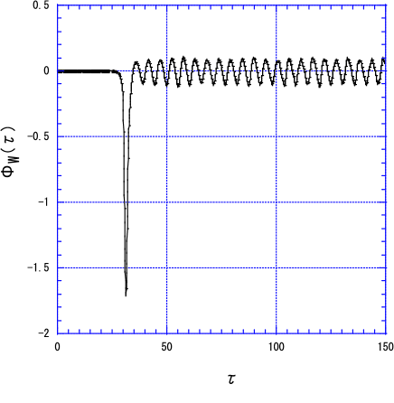
Figure 4: Time evolution of a scalar field on one moving wall for $\upsilon=0.4,\ {\lambda}=1.0$. The value of the scalar field is given by $\Phi_{\rm W}(\tau)=\Phi(t,y_{\rm W}(t))$, where $y_{\rm W}(t)$ is the position of the wall and $\tau$ is the proper time on the wall.

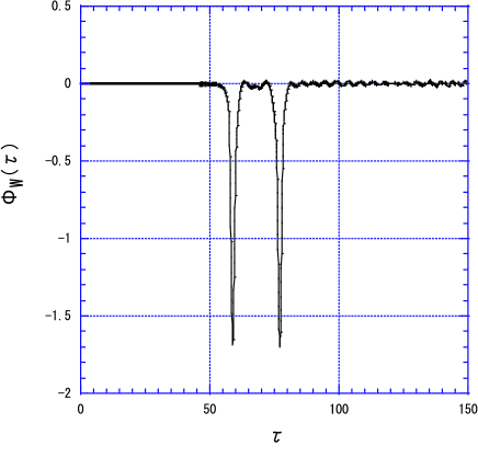
Figure 5: Time evolution of a scalar field $\Phi_{\rm W}(\tau)$ on one moving wall for $\upsilon=0.2,\ {\lambda}=1.0$.

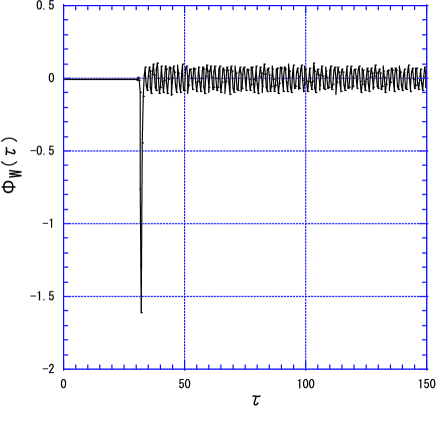
Figure 6: Time evolution of a scalar field $\Phi_{\rm W}(\tau)$ on one moving wall for $\upsilon=0.4,\ {\lambda}=10$.

We also show the results for different values of the coupling constant $\lambda$ in Figs. 6 and 7 ($\lambda=10$). If Fig. 6 we find that when $\lambda$ gets larger as $\lambda=10$, the spike of $\Phi_{\rm W}$ becomes sharp. The same thing happens in the case of two bounce (see Fig. 7).

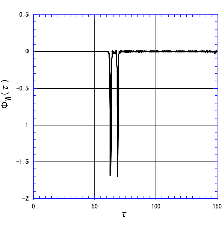
Figure 7: Time evolution of a scalar field $\Phi_{\rm W}(\tau)$ on one moving wall for $\upsilon=0.2,\ {\lambda}=10$.

In Figs. 4-7, we find that $\Phi_{\rm W}$ begins to oscillate after the collision. We also find that the period of these oscillations in Figs. 6 and 7 is shorter that those in Figs. 4 and 5. One may wonder whether this oscillation is realistic or not. This oscillation, however, turns out not to be a numerical error but a real oscillation of the domain wall. In Appendix C, using perturbation analysis we show there is one stable oscillation around the kink solution $\Phi_{K}(y)$. We expect that the oscillation is excited by the collision. In fact, the amplitude of the oscillation increases as the incident velocity $\upsilon$ increases. In large velocity limit ($\upsilon\mbox{\raisebox{-4.30554pt}{$\stackrel{{\scriptstyle\textstyle>}}{{\textstyle\sim}}$}}0.6$), we find $\Phi_{\infty}^{2}\approx 0.18(\gamma-1)$, where $\Phi_{\infty}$ is the amplitude of the post-oscillation.

Since the scalar field on the domain wall oscillates as $\Phi_{\rm W}\approx\Phi_{\infty}\cos\sigma\tau$ after the collision, our wave equation (15) would be rewritten as

$$\ddot{\psi_{k}}+\left[k^{2}+{1\over 2}\bar{g}^{2}\Phi_{\infty}^{2}\left(1+\cos 2\sigma\tau\right)\right]\psi_{k}=0\ ,$$ (28)

where $\sigma=\sqrt{3/2}\lambda^{1/2}$ is the eigenvalue of the perturbation eigen function, it is so-called Methieu equation.

From this equation, we may wonder whether we can ignore this oscillation when we evaluate particle production rate. In fact, when we discuss a preheating mechanism via a parametric resonance with a similar oscillating behaviorpreheating , in conventional cosmology22 as well as brane world cosmology tujikawa . It is known that for Methieu equation, there is an exponential instability ${\psi_{k}}\propto\exp(\mu_{k}t)$ within a set of resonance bands, where $\mu_{k}=\bar{g}\Phi^{2}_{\infty}/8$. This instability corresponds to an exponential growth of created particles, which is essential in the preheating mechanism. In order to get a successful particle production by this resonance instability, however, we have to require large value of $\bar{g}^{2}\Phi_{\infty}^{2}$. However, in the present simulation, it is rather small, e.g. $\Phi_{\infty}\sim 0.1$ for the case of $\upsilon=0.4$. Hence, we may ignore such a particle production by a parametric resonance in the present calculation. However, if the incident velocity is very fast such as a speed of light, we may find a large oscillation. Then we could have an instant preheating process by the domain wall collision. We also wonder whether or not the standard reheating mechanism due to the decay of oscillating scalar field is effective. In this case, we have to evaluate the decay rate $\Gamma_{\phi}$ to other particles. Since $\Gamma_{\phi}\propto\bar{g}^{4}$, we expect that the reheating temperature is proportional to $\bar{g}^{2}$, which is enough small to be ignored. Note that there is another factor which reduces the decay rate in the case that the potential is not a spontaneous symmetry breaking typepreheating .

In what follows, we ignore the creation due to post-oscillation stage. Hence, we just follow the procedure shown in the previous subsection. Using the evolution of the scalar field $\Phi_{\rm W}$, we calculate the Bogolubov coefficients $\alpha_{k}$ and $\beta_{k}$. In Table 1, we show the results for three different parameters; $\upsilon$ (the incident velocity), $\lambda$ (the self-coupling constant of the scalar field), and $\bar{g}$ (the coupling constant to a particle $\psi$).

$\bar{g}$	$\upsilon$	${\lambda}$	$d$	$N_{b}$	$n$	$\rho$
	0.4	1.0	1.414	1	3.69$\times 10^{-7}$	2.05$\times 10^{-7}$
$0.01$		10	0.447		1.16$\times 10^{-7}$	2.05$\times 10^{-7}$
	0.2	1.0	1.414	2	7.19$\times 10^{-7}$	3.90$\times 10^{-7}$
		10	0.447		2.26$\times 10^{-7}$	3.91$\times 10^{-7}$
	0.4	1.0	1.414	1	3.57$\times 10^{-3}$	2.01$\times 10^{-3}$
0.1		10	0.447		1.16$\times 10^{-3}$	2.05$\times 10^{-3}$
	0.2	1.0	1.414	2	6.65$\times 10^{-3}$	3.81$\times 10^{-3}$
		10	0.447		2.24$\times 10^{-3}$	3.88$\times 10^{-3}$

Table 1: The number and energy densities ($n$ and $\rho$) of created particles for the typical values of the coupling $\bar{g}$, the incident velocity $\upsilon$ and the self-coupling $\lambda$. $d=\sqrt{2/\lambda}$ and $N_{b}$ denote the width of the wall and the number of bounces at the collision, respectively.

From this Table, we find the following three features:
(1) The produced energy density $\rho$ depends very much on $\bar{g}$. We study two cases with $\bar{g}=0.01$ and $0.1$. The energy density for $\bar{g}=0.1$ is $10^{4}$ times larger than that for $\bar{g}=0.1$, which means that $\rho$ is proportional to $\bar{g}^{4}$.
(2) The energy density $\rho$ for $\upsilon=0.2$ is twice larger than that for $\upsilon=0.4$. It may be so because the bounce occurs twice for $\upsilon=0.2$, while once for $\upsilon=0.4$.
(3) The energy density is less sensitive to $\lambda$.

We also investigate for several different initial velocities because the collisional process is very sensitive to its incident velocity. We analyze many cases with two bounces, with three bounces, with four bounces, $\cdots$ in the range $\upsilon=0.2$-$0.25$ as shown in Appendix B. Using those numerical data, we also evaluate the number and energy densities of the particles created at the collision. The results are summarized in Table 2.

From this Table, we confirm the above three features (1)-(3). In particular, it becomes more clear that the energy density is proportional to the number of bounce $N_{b}$.

We can summarize our results by the following empirical formula

$$n \approx 25d\bar{g}^{4}N_{b}\ ,$$ (29)

$$\rho \approx 20\bar{g}^{4}N_{b}\ .$$ (30)

If this energy of the particles is thermalized by interaction and thermal equilibrium state is realized, we can estimate the reheating temperature by

$$\rho={\pi^{2}\over 30}g_{\rm eff}T_{\rm R}^{4}\,,$$ (31)

where $g_{\rm eff}$ is the effective number of degrees of freedom of particles. Hence we find the reheating temperature by the domain wall collision as

$$T_{\rm R} = \left({\pi^{2}\over 30}\right)^{-1/4}g_{\rm eff}^{-1/4}\rho^{1/4}$$ (32)

$$\approx 0.88\times\left({g_{\rm eff}\over 100}\right)^{-1/4}~{}\bar{g}~{}N_{b}^{1/4}\,.$$

$N_{b}$	$\upsilon$	${\lambda}$	$d$	$n$	$\rho$
	0.225	1.0	1.414	7.03$\times 10^{-7}$	3.72$\times 10^{-7}$
2		10	0.447	2.21$\times 10^{-7}$	3.71$\times 10^{-7}$
	0.238	1.0	1.414	7.08$\times 10^{-7}$	3.78$\times 10^{-7}$
		10	0.447	2.23$\times 10^{-7}$	3.78$\times 10^{-7}$
	0.2062	1.0	1.414	1.10$\times 10^{-6}$	6.07$\times 10^{-7}$
		10	0.447	3.45$\times 10^{-7}$	6.06$\times 10^{-7}$
	0.2049	1.0	1.414	1.09$\times 10^{-6}$	6.01$\times 10^{-7}$
3		10	0.447	3.43$\times 10^{-7}$	6.01$\times 10^{-7}$
	0.2298	1.0	1.414	1.10$\times 10^{-6}$	6.04$\times 10^{-7}$
		10	0.447	3.43$\times 10^{-7}$	6.02$\times 10^{-7}$
	0.22933	1.0	1.414	1.09$\times 10^{-6}$	6.03$\times 10^{-7}$
		10	0.447	3.44$\times 10^{-7}$	6.01$\times 10^{-7}$
	0.229283	1.0	1.414	1.47$\times 10^{-6}$	8.10$\times 10^{-7}$
4		10	0.447	4.61$\times 10^{-7}$	8.09$\times 10^{-7}$
	0.2292928	1.0	1.414	1.47$\times 10^{-6}$	8.16$\times 10^{-7}$
		10	0.447	4.62$\times 10^{-7}$	8.17$\times 10^{-7}$

Table 2: The number and energy densities ($n$ and $\rho$) of created particles with respect to the number of bounces $N_{b}$. $\upsilon$ and $d$ are the incident velocity and the width of the wall, respectively. We set $\bar{g}=0.01$.

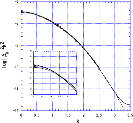
Figure 8: Spectrum of the created particles at the collision. We plot $\log|\beta_{k}|^{2}k^{2}$ with respect to $k$ for $\upsilon=0.4,\ {\lambda}=1.0,{\bar{g}}=10^{-2}$. The gaussian distribution is plotted by a dotted line, which gives a good approximation for $k\leq 3$. In the small box, we enlarge the low frequency region ($k\leq 1$) to see the deviation from the gaussian distribution.

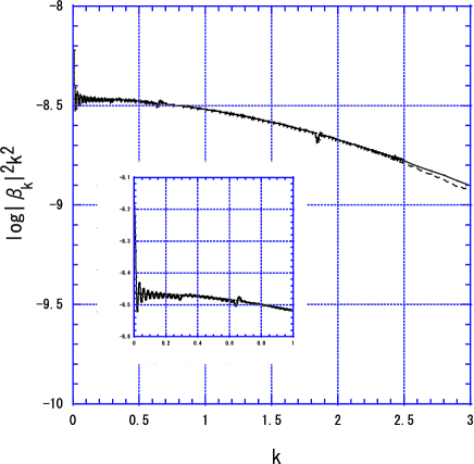
Figure 9: Spectrum of the created particles at the collision. We plot $\log|\beta_{k}|^{2}k^{2}$ with respect to $k$ for $\upsilon=0.4,\ {\lambda}=10,{\bar{g}}=10^{-2}$. The gaussian distribution is plotted by a dotted line, which gives a good approximation for $k\leq 2.5$. In the small box, we enlarge the low frequency region ($k\leq 1$) to see the deviation from the gaussian distribution.

In order to see more details, in Figs. 8 and 9, we show a spectrum of the produced particles of number density $n$, i.e.

$$n=\int_{0}^{\infty}dk~{}n_{k}~{}~{}{\rm with}~{}~{}n_{k}=4\pi|\beta_{k}|^{2}k^{2}\ .$$ (33)

The spectrum $n_{k}$ is well fitted as a gaussian distribution as

$$n_{k}\approx 4\pi Ae^{-{k^{2}\over 2k_{0}^{2}}}\,,$$ (34)

where $k_{0}=0.73$ and $A=3.12\times 10^{-8}$ for Fig. 10 and $k_{0}=2.04$ and $A=3.43\times 10^{-9}$ for Fig. 11, although there is small deviation partially. These parameters can be described by physical quantities as $k_{0}\approx 1/d$ and $A\approx\Phi_{0}d^{2}\bar{g}^{4}$. The reason is well understood. $k_{0}\approx 1/d$ means that the typical wave number is given by the width of the scalar field when domain walls collide (see Fig. 3). As for $\beta$, it corresponds to the ”reflection” coefficient of the ”potential” given by Figs. 4-7 and then it will be proportional to the coupling constant $\bar{g}^{2}$, and the reflection rate ($|\beta|^{2}$) will be related to the potential depth $\Phi_{0}$ and the square of the width $d^{2}$.

Integrating the fitting spectrum (34), we obtain

$$n = \int_{0}^{\infty}n_{k}dk=(2\pi)^{3/2}\Phi_{0}d\bar{g}^{4}\approx 25d\bar{g}^{4}\ ,$$ (35)

$$\rho = \int_{0}^{\infty}n_{k}\omega_{k}dk=4\pi\Phi_{0}\bar{g}^{4}\approx 20\bar{g}^{4}\ ,$$ (36)

which values are exactly the same as those obtained by numerical integration in the case with one bounce (see Eqs. (29) and (30)). We expect that they are enhanced by the factor $N_{b}$ when we find $N_{b}$ bounces at the collision.

Therefore, although we obtain the particle creation numerically, the result is easily understood and summarized by a simple formula.

IV summary and discussion

We study the particle production at the collision of two domain walls in 5D Minkowski spacetime. This may provide the reheating mechanism of an ekpyrotic (or cyclic) brane universe, in which two BPS branes collide and evolve into a hot big bang universe. We evaluate a production rate of particles confined to the domain wall. The energy density of created particles is approximate as $\rho\approx 4\pi\Phi_{0}\bar{g}^{4}N_{b}$ where $\Phi_{0}$ is the maximum amplitude of $\Phi_{\rm W}$, $N_{b}$ is the number of bounce at the collision and $\bar{g}$ is a coupling constant of a particle to the scalar field of a domain wall. If this energy is converted into standard matter fields, we find the reheating temperature as $T_{\rm R}\approx 0.88\times\bar{g}~{}N_{b}^{1/4}\left({g_{\rm eff}/100}\right)^{-1/4}$. We find that the particle creation is affected more greatly by a coupling constant $\bar{g}$ than the other two parameters $\upsilon$ and $\lambda$. The initial velocity changes the collision process, that is the number of bounce at the collision, but this is less sensitive to the temperature. The thickness of a domain wall $d$ (or a self-coupling constant $\lambda$) changes the width of potential $\Phi_{\rm w}^{2}(\tau)$ of a particle field ($\psi$), and it changes a typical energy scale of created particles, which is estimated as $\omega\sim 1/d$.

In order to find a successful reheating, a reheating temperature must be higher than $10^{2}$ GeV, because we wish to explain the baryon number generation at the electro-weak energy scale21 . Since Eq. (32) is written in the following form;

$$m_{\eta} \approx 1.1N_{b}^{-1/4}\bar{g}^{-1}{T_{\rm R}}$$

$$\approx 1.1\times 10^{7}[{\rm GeV}]\ N_{b}^{-1/4}\left({\bar{g}\over 10^{-5}}\right)^{-1}\left({T_{\rm R}\over 10^{2}{\rm GeV}}\right)\ ,$$ (37)

we find a constraint on a fundamental energy scale $m_{\eta}$ as $m_{\eta}\mbox{\raisebox{-4.30554pt}{$\stackrel{{\scriptstyle\textstyle>}}{{\textstyle\sim}}$}}1.1\times 10^{7}~{}{\rm GeV}$ for $\bar{g}=10^{-5}$ and $m_{\eta}\mbox{\raisebox{-4.30554pt}{$\stackrel{{\scriptstyle\textstyle>}}{{\textstyle\sim}}$}}1.1\times 10^{4}~{}{\rm GeV}$ for $\bar{g}=10^{-2}$, which are slightly larger than TeV scale. Here we assume ${g_{\rm eff}}=100$

In the present work, we consider the 3-dimensional domain walls in the 5-dimensional Minkowski space and show that the particle production at the two-wall collision may provide a successful mechanism for reheating in the ekpyrotic universe. In a string/M theory, however, we expect higher dimensions, e.g. 10 or 11. If we compactify it to the effective 5-dimensional spacetime, our work can be applicable to such a mode. Moreover, if we discuss a collision of a $p$-dimensional walls (branes) in $(p+2)$-dimensional spacetime, our approach can also be extended.

In this paper, we have not taken account of effects from a background spacetime. We are planning to study how such a generalization affects the present results about particle creation at the collision.

Appendix A Numerical method

For our numerical analysis of the domain wall collision, we solve the partial differential equation (3) on discrete spatial grids with a periodic boundary condition. The scalar field on the grid points is defined by ${\Phi}_{n}(t)={\Phi}({y}_{n},t)$, where ${y}_{n}=n\triangle y$, for $n=1,2,\ldots,N$. We use the fourth-order center difference scheme to approximate the second spatial derivative 12 as

$$\frac{\partial^{2}{\Phi}_{n}}{\partial{y}^{2}}= \frac{1}{12(\triangle{y})^{2}}\left[-{\Phi}_{n-2}+16{\Phi}_{n-1}-30{\Phi}_{n}\right.$$

$$\left.~{}~{}~{}~{}~{}+16{\Phi}_{n+1}-{\Phi}_{n+2}\right]+O((\triangle{y})^{4})\ .$$ (38)

This leads to a set of $N$ coupled second-order ordinary differential equation (ODE’s) for the ${\Phi}_{n}$, i.e.

$$\frac{d^{2}{\Phi}_{n}}{d{t}^{2}}= \frac{1}{12(\triangle{y})^{2}}\left[-{\Phi}_{n-2}+16{\Phi}_{n-1}-30{\Phi}_{n}\right.$$

$$\left.+16{\Phi}_{n+1}-{\Phi}_{n+2}\right]-{\lambda}{\Phi}_{n}({\Phi}^{2}_{n}-1)\ .$$ (39)

The ODE’s (39) are solved using a forth-order Runge-Kutta scheme, and so our numerical algorithm is accurate to fourth order both in time and in space, with error of $O((\triangle{y})^{4})$ and $O((\triangle{t})^{4})$. For the boundaries, we set the left and right grid boundaries at ${y}_{L}=-40$ and ${y}_{R}=+40$, and impose the condition as ${\Phi}({y}={y}_{L},t)={\Phi}({y}={y}_{R},t)=-1$ . The grid number is $N=8000$ with the grid size of $\triangle{y}=1.0\times 10^{-2}$. The initial position of a wall $y_{0}$ is set by ${y}_{0}=|{y}_{L}+({y}_{R}-{y}_{L}+1)/3|=13$, equivalently, one-third of the numerical range. For time steps, we set $\triangle{t}=0.7\times\triangle{y}$.

As for the particle production process, we have to solve the second-order ordinary differential equations (15) for each wave number ${k}$. By using the fourth-order Runge-Kutta scheme, we solve them for the wave number $k$ of $0<k<100$ with the width $\triangle{k}=1.0\times 10^{-3}$. We estimate $|\beta_{k}|^{2}$ in the equation (21). Defining the functions like these

$$W_{1} \equiv \psi_{k}\dot{\psi}^{*}_{k}-\psi^{*}_{k}\dot{\psi}_{k}\ ,$$ (40)

$$W_{2} \equiv \psi_{k}\dot{\psi}^{*}_{k}+\psi^{*}_{k}\dot{\psi}_{k}\ ,$$ (41)

$$W_{3} \equiv \psi_{k}\psi_{k}^{*}\ ,$$ (42)

we use the formula

$$|\beta_{k}|^{2}=\frac{(W_{3}-W_{1}/2i\omega)^{2}+(W_{2}/2\omega)^{2}}{4W_{3}}\ ,$$ (43)

to evaluate $|\beta_{k}|$.

Appendix B Numerical examples of several bounces at the collision

We depict some numerical examples which show several bounces at the collision. First we show two typical examples in Fig. 10.

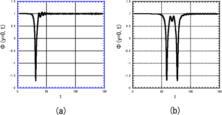
Figure 10: Time evolution of $\Phi$ field at $y=0$ are depicted for (a) $\upsilon=0.4\ {\lambda}=1.0$ and (b) $\upsilon=0.2,\ {\lambda}=1.0$. The bounce occurs once for a large velocity (a), while Two bounces are found for the slower velocity.

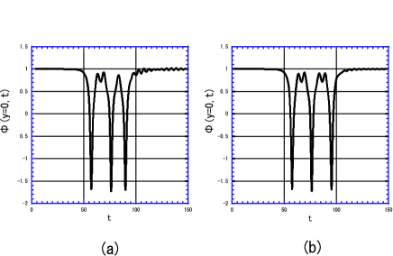
Figure 11: Time evolution of $\Phi$ field at $y=0$ are depicted for (a) $\upsilon=0.2062\ {\lambda}=1.0$ and (b) $\upsilon=0.2049,\ {\lambda}=1.0$. Three bounces are found.

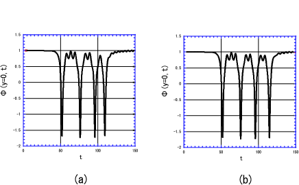
Figure 12: Time evolution of $\Phi$ field at $y=0$ are depicted for (a) $\upsilon=0.229283\ {\lambda}=1.0$ and (b) $\upsilon=0.2292928,\ {\lambda}=1.0$. Four bounces are found.

The figures show the behaviors of the scalar field $\Phi$ at $y=0$ with respect to $t$. Initially, when two domain walls locate at large distance, the value of the scalar field at $y=0$ is $1$. Then two walls approach and collide. At this point the value of $|\Phi-1|$ increases. After the collision, it again decreases to an initial value. We find some small oscillation around a domain wall structure which is excited by the collision.

From Fig. 10, we find there is one bounce for $\upsilon=0.4$, while a bounce occurs twice for $\upsilon=0.2$. In fact, the results are very much sensitive to the incident velocities as shown in fractal .

Here we present several examples to show how the behaviors of the scalar field depend on $\upsilon$, which confirm the previous works.

In Figs. 11 (a) and (b), we show the case for $\upsilon=0.2062$ and $\upsilon=0.2049$, respectively. We find three bounces at the collision. Four-bounce solutions are depicted in Figs. 12 (a) ($\upsilon=0.229283$) and (b) ($\upsilon=0.2292928$). These calculation shows that the detail collisional process is very sensitive to the incident velocity.

Appendix C perturbations of a domain wall

We show that the oscillation we find in Sec III.2, is a proper oscillation around a static stable domain wall. To show it, we perturb the static domain wall solution (4) as

$$\Phi=\Phi_{K}(y)+\delta\Phi(t,y)\ .$$ (44)

In this appendix, we use the dimensionless variables rescaled by $\eta$. Substituting this into Eq. (3) and linearizing it, we obtain

$$\delta\ddot{\Phi}-\delta\Phi^{\prime\prime}+\lambda(3\Phi_{K}^{2}-1)\delta\Phi=0\ .$$ (45)

Setting

$$\delta\Phi=e^{-i\sigma t}F(y)\ ,$$ (46)

and introducing new variable $\bar{y}=\tanh(y/d)$, we rewrite Eq. (45) as

$$(1-\bar{y}^{2}){d^{2}F\over d\bar{y}^{2}}-2\bar{y}{dF\over d\bar{y}}+2\left[3-\frac{2-\sigma^{2}/\lambda}{1-\bar{y}^{2}}\right]F=0\ .$$ (47)

The solution is given by the associated Legendre function. Imposing the boundary condition ($F\to 0$ as $\bar{y}\to\infty$), we have two regular solutions; $F(\bar{y})=P_{2}^{\,2}(\bar{y})$ with $\sigma=0$ and $P_{2}^{\,1}(\bar{y})$ with $\sigma=\sqrt{3/2}\lambda^{1/2}$.

For the former mode, it just corresponds to a boost of a kink solution in the $y$ direction, because we find $F(y)\approx\Phi_{K}(y)-\Phi_{K}(y-dy)$. The latter one is the oscillation mode which we find in Sec II.2. In fact, taking the average over 10 cycles in the oscillation after the collision in Fig. 4, we obtain the mean angular frequency is about $1.17$, which is very close to $\sigma=\sqrt{3/2}\sim 1.22$. The ratio is about 0.96. We also evaluate the angular frequency for other cases. We find $1.33=1.09\sigma$ for Fig. 5, $3.67=0.95\sigma$ for Fig. 6, and $4.18=1.08\sigma$ for Fig. 7. From the figures, we also find that the amplitude of oscillation gets larger as the incident velocity is faster. This is because the excitation energy of a wall at the collision will be large for a large velocity.

We then conclude that the oscillations after the collision of two domain walls is the proper oscillations around a stable domain wall.

References

- (1) A. Linde, Particle Physics and Inflationary Cosmology (Harwood, 1990).
- (2) E. W. Kolb and M. S. Turner, The Early Universe (Westview Press, Chicago, United States of America, 1990).
-
(3)
K. Akama, Lect. Notes Phys. 176, 267 (1982);
V. A. Rubakov and M. E. Shaposhnikov, Phys. Lett. 125B, 136 (1983);
M. Visser, ibid. 159B, 22 (1985). -
(4)
I. Antoniadis, Phys. Lett. 246B, 377 (1990);
N. Arkani-Hamed, S. Dimopoulos, and G. Dvali, ibid. 429B, 263 (1998);
I. Antoniadis, N. Arkani-Hamed, S. Dimopoulos, and G. Dvali, ibid. 436B, 257 (1998). -
(5)
P. Hoava and E. Witten, Nucl. Phys. B460, 506 (1996);
ibid. B475, 94 (1996). - (6) J. Polchinski, String Theory I & II (Cambridge Univ. Press, Cambridge, 1998).
- (7) J. Polchinski, Phys. Rev. Lett. 75, 4724 (1995).
- (8) L. Randall and R. Sundrum, Phys. Rev. Lett. 83, 4690 (1999).
-
(9)
P. Bintruy, C. Deffayet and D. Langlois, Nucl. Phys. B 565, 269 (2000);
P. Bintruy, C. Deffayet, U. Ellwanger and D. Langlois, Phys. Lett. B 477, 285 (2000). -
(10)
C. Csaki, M. Graesser, C. Kolda and J. Terning Phys. Lett. B 462,
34 (1999);
N. Kaloper, Phys. Rev. D 60, 123506 (1999);
T. Nihei, Phys. Lett. B 465, 81 (1999);
H. S. Reall, ibid. 103506 (1999). -
(11)
A. Lukas, B. A. Ovrut, K. S. Stelle,
and D. Waldram, Phys. Rev. D
59, 086001 (1999);
A. Lukas, B. A. Ovrut, and D. Waldram, ibid. D 60 086001 (1999). -
(12)
K. Maeda,
Prog. Theor. Phys. Suppl. 148, 59 (2003);
K. Maeda, Lect. Notes Phys. 646, 323 (2004). -
(13)
R. Maartens,
arXiv:gr-qc/0101059;
R. Maartens, Prog. Theor. Phys. Suppl. 148, 213 (2003);
R. Maartens, arXiv:gr-qc/0312059. -
(14)
D. Langlois,
arXiv:gr-qc/0207047;
D. Langlois, Prog. Theor. Phys. Suppl. 148, 181 (2003). -
(15)
P. Brax and C. van de Bruck,
Class. Quant. Grav. 20, R201 (2003);
P. Brax, C. van de Bruck and A. C. Davis, arXiv:hep-th/0404011. -
(16)
T. Shiromizu, K. Maeda, and M. Sasaki, Phys. Rev.
D 62, 0244012 (2000);
S. Mukohyama, T. Shiromizu and K. Maeda, ibid. D 62, 024028 (2000). - (17) K. Maeda and D. Wands, Phys. Rev. D 62, 124009 (2000).
-
(18)
J. Khoury, B. A. Ovrut, P. J. Steinhardt and N. Turok,
Phys. Rev. D 64, 123522 (2001);
J. Khoury, B. A. Ovrut, N. Seiberg, P. J. Steinhardt and N. Turok, ibid. D 65, 086007 (2002);
J. Khoury, B. A. Ovrut, P. J. Steinhardt and N. Turok, ibid. D 66, 046005 (2002);
A. J. Tolley and N. Turok, ibid. D 66, 106005 (2002). -
(19)
P. J. Steinhardt and N. Turok,
Phys. Rev. D 65, 126003 (2002);
J. Khoury, P. J. Steinhardt and N. Turok, Phys. Rev. Lett. 92, 031302 (2004). - (20) D. H. Lyth, Phys. Lett. B 524, 1 (2002).
-
(21)
R. Brandenberger and F. Finelli,
JHEP 0111, 056 (2001);
F. Finelli and R. Brandenberger, Phys. Rev. D 65, 103522 (2002). -
(22)
J. Martin, P. Peter, N. Pinto Neto and D. J. Schwarz,
Phys. Rev. D 65, 123513 (2002);
P. Peter and N. Pinto-Neto, ibid. D 66, 063509 (2002);
J. Martin, P. Peter, N. Pinto-Neto and D. J. Schwarz, ibid. D 67, 028301 (2003). -
(23)
S. Tsujikawa,
Phys. Lett. B 526, 179 (2002);
S. Tsujikawa, R. Brandenberger and F. Finelli, Phys. Rev. D 66, 083513 (2002);
L. E. Allen and D. Wands, arXiv:astro-ph/0404441. -
(24)
J. Martin, G. N. Felder, A. V. Frolov, M. Peloso and L. Kofman,
Phys. Rev. D 69, 084017 (2004);
J. Martin, G. N. Felder, A. V. Frolov, L. Kofman and M. Peloso, arXiv:hep-ph/0404141. - (25) G. Dvali and A. Vilenkin, Phys. Rev. D 67, 046002 (2003).
-
(26)
N. D. Antunes, E. J. Copeland, M. Hindmarsh and A. Lukas,
Phys. Rev. D 68, 066005 (2003);
N. D. Antunes, E. J. Copeland, M. Hindmarsh and A. Lukas, ibid. D 69, 065016 (2004). -
(27)
M. Eto and N. Sakai,
Phys. Rev. D 68, 125001 (2003);
M. Eto, S. Fujita, M. Naganuma and N. Sakai, ibid. D 69, 025007 (2004). - (28) L. Windrow, Phys. Rev. D 40, 1002 (1989).
- (29) P. Anninos, S. Oliveira and R. A. Matzner, Phys. Rev. D 44, 1147 (1991).
- (30) D. K. Campbell, J. F. Schonfeld and C. A. Wingate, Physica 9D, 1 (1983).
- (31) V. Silveira, Phys. Rev. D 38, 3823 (1988).
- (32) T. I. Belova and A. E. Kudryavtsev, Physica D 32, 18 (1988).
- (33) N. D. Birrell and P. C. W. Davies, Quantum Fields In Curved Space (Cambridge University Press, Cambridge, England, 1982).
-
(34)
L. Kofman, A. D. Linde and A. A. Starobinsky,
Phys. Rev. Lett. 73, 3195 (1994);
L. Kofman, A. D. Linde and A. A. Starobinsky, Phys. Rev. D 56, 3258 (1997). - (35) S. Tsujikawa, K. Maeda and S. Mizuno, Phys. Rev. D 63, 123511 (2001).
- (36) R. W. Hornbeck, Numerical Methods (Prentice-Hall, Englewood Cliffs, NJ, 1975).