Abstract

Spherically symmetric solutions of the $SU(5)$ Einstein-Yang-Mills-Higgs system are constructed using the harmonic map ansatz [1]. This way the problem reduces to solving a set of ordinary differential equations for the appropriate profile functions.

1 Introduction

Magnetic monopoles are of diverse interest since they are predicted from grant unified theories (GUT) and embody a rich mathematical structure. Also, they appear in non-perturbative field theories and provide a new perspective on particle physics phenomenology. In particular, the $SU(5)$ gauge group plays a central role in GUT and thus it is natural to classify the magnetic monopoles related to this model [2]. A few years ago, the effects of gravitation on monopoles were (also) considered [3] and revealed a rich pattern of solutions (including the occurrence of black holes) related to the gravitational parameter: $\alpha^{2}\equiv Gv$ where $G$ denotes Newton constant and $v\in\hbox{\upright\hbox to0.0pt{I\hss}\kern 1.7ptR}$ is the vacuum expectation value of the Higgs field. More recently, a new interest for $SU(5)$ monopoles was stimulated by the discovery of a deep analogy between their magnetic charges and the electric charges in one generation of elementary particles [4]. This originated several new papers on the topic, see e.g. [5, 6] and references therein. Here we use the harmonic map ansatz [1], recently applied to $SU(3)$ gravitating monopole [7], in order to construct their $SU(5)$ counterparts. A similar analysis has been applied for deriving $SU(5)$ solutions (including black holes) which are embeddings of the $SU(2)$ ones [8] . However, the solutions constructed here are non-embedded of the $SU(2)$ ones and correspond to monopole-antimonopole configurations.

The $SU(5)$ Einstein-Yang-Mills-Higgs action is given by:

$$S=\int\left[\frac{R}{16\pi G}-\frac{1}{2}\mbox{tr}\left(F_{\mu\nu}\,F^{\mu\nu}\right)-\mbox{tr}\left(D_{\mu}\Phi\,D^{\mu}\Phi\right)-V(\Phi)\right]\sqrt{-g}\,d^{4}x$$ (1)

where the potential is of the form [4]:

$$V(\Phi)=-\lambda_{1}\mbox{tr}(\Phi^{2})+\lambda_{2}\left(\mbox{tr}(\Phi^{2})\right)^{2}+\lambda_{3}\mbox{tr}(\Phi^{4})-V_{min}.$$ (2)

Here $g$ denotes the determinant of the metric while the field strength tensor is defined by: $F_{\mu\nu}=\partial_{\mu}A_{\nu}-\partial_{\nu}A_{\mu}+[A_{\mu},A_{\nu}]$ and the covariant derivative of the Higgs field reads: $D_{\mu}\Phi=\partial_{\mu}\Phi+[A_{\mu},\Phi].$ The matrix $\eta$ represents a constant matrix of the form: $\eta=iv{\bf 1}_{N}$, where ${\bf 1}_{N}$ denotes the unit matrix in $N$ dimensions. Finally, $V_{min}=-15\lambda_{1}^{2}/(60\lambda_{2}+14\lambda_{3})$ has been subtracted due to the finiteness of the energy.

The boundary conditions are such that the energy is finite and the Higgs field at infinity is a given constant matrix $\Phi(0,0,\infty)=i\Phi_{0}$

$$\Phi_{0}=\mbox{diag}\left(\kappa_{1},\kappa_{2},\kappa_{3},\kappa_{4},\kappa_{5}\right)$$ (3)

in a chosen direction (while since $\Phi\in su(5)$: $\sum_{i}^{5}\kappa_{i}=0$). In addition, the asymptotic values $G_{0}$ of the magnetic charge $G=(1+|z|^{2})^{2}F_{z\bar{z}}$ is given by

$$G_{0}=G(0,0,1)=\mbox{diag}\left(n_{1},n_{2}-n_{1},n_{3}-n_{2},n_{4}-n_{3},-n_{4}\right).$$ (4)

Variation of (1) with respect to the metric $g^{\mu\nu}$ leads to the Einstein equations

$$R_{\mu\nu}-\frac{1}{2}g_{\mu\nu}R=8\pi G\,T_{\mu\nu}$$ (5)

with the stress-energy tensor $T_{\mu\nu}=g_{\mu\nu}{\cal L}-2\frac{\partial{\cal L}}{\partial g^{\mu\nu}}$ given by

$$T_{\mu\nu}\!\!\! = \!\!\!\mbox{tr}\left(2D_{\mu}\Phi\,D_{\nu}\Phi-g_{\mu\nu}D_{\alpha}\Phi\,D^{\alpha}\Phi\right)\!+\!2\mbox{tr}\left(g^{\alpha\beta}\,F_{\mu\alpha}F_{\nu\beta}-\frac{1}{4}g_{\mu\nu}\,F_{\alpha\beta}F^{\alpha\beta}\right)-g_{\mu\nu}V(\Phi).\hskip 14.22636pt\hskip 14.22636pt$$ (6)

In what follows we consider the static Einstein-Yang-Mills-Higgs equations in order to construct their $SU(5)$ spherically symmetric and purely magnetic (ie $A_{0}=0$) solutions based on the harmonic map ansatz first introduced in [1].

2 Spherical Symmetry

The starting point of our investigation is the introduction of the coordinates $r,z,{\bar{z}}$ on $\hbox{\upright\hbox to0.0pt{I\hss}\kern 1.7ptR}^{3}$. In terms of the usual spherical coordinates $r,\theta,\phi$ the Riemann sphere variable $z$ is given by $z=e^{i\phi}\tan(\theta/2)$. In this system of coordinates the Schwarzschild-like metric reads:

$$ds^{2}=-A^{2}(r)B(r)dt^{2}+\frac{1}{B(r)}dr^{2}+\frac{4r^{2}}{(1+|z|^{2})^{2}}\,dzd\bar{z},\hskip 14.22636ptB(r)=1-\frac{2m(r)}{r},$$ (7)

where $A$ and $B$ are the metric functions which are real and depend only on the radial coordinate $r$, and $m(r)$ is the mass function. The (dimensionfull) mass of the solution is given by $m_{\infty}\equiv m(\infty)$. For this metric the square-root of the determinant takes the simple form:

$$\sqrt{-g}=iA(r)\,\frac{2r^{2}}{(1+|z|^{2})^{2}}.$$ (8)

Then, the action (1) simplifies to

$$S\!\!\! = \!\!\!\!\!\int\bigg{\{}\frac{B(1+|z|^{2})^{2}}{r^{2}}\mbox{tr}\left(|F_{rz}|^{2}\right)+\frac{(1+|z|^{2})^{4}}{4r^{4}}\mbox{tr}\left(F_{z\bar{z}}^{2}\right)-B\,\mbox{tr}\left((D_{r}\Phi)^{2}\right)-\frac{(1+|z|^{2})^{2}}{r^{2}}\mbox{tr}\left(|D_{z}\Phi|^{2}\right)$$ (9)

$$\,\,\,\,\,\,-V(\Phi)\bigg{\}}\sqrt{-g}\,r^{2}\,drdt$$

and the matter equations can be obtained by its variation with respect to the matter fields.

In addition, the Einstein equations (5) take the form:

$$\frac{2}{r^{2}}\,m^{\prime}=8\pi G\,T^{0}_{0},\hskip 14.22636pt\hskip 14.22636pt\frac{2}{r}\frac{A^{\prime}}{A}\,B=8\pi G\,\left(T^{0}_{0}-T^{r}_{r}\right)$$ (10)

where prime denotes the derivative with respect to $r$, and

$$\!\!\!\!\!\!\!\!\!T_{0}^{0}=\frac{(1+|z|^{2})^{4}}{4r^{4}}\mbox{tr}\left(F_{z\bar{z}}^{2}\right)-\frac{B(1+|z|^{2})^{2}}{r^{2}}\mbox{tr}\left(|F_{rz}|^{2}\right)-B\,\mbox{tr}\left((D_{r}\Phi)^{2}\right)-\frac{(1+|z|^{2})^{2}}{r^{2}}\mbox{tr}\left(|D_{z}\Phi|^{2}\right)-V(\Phi)\hskip 14.22636pt\hskip 14.22636pt\hskip 14.22636pt\hskip 14.22636pt$$

$$\!\!\!\!\!\!\!\!\!T^{0}_{0}-T^{r}_{r}=-\frac{2B(1+|z|^{2})^{2}}{r^{2}}\mbox{tr}\left(|F_{rz}|^{2}\right)-2B\,\mbox{tr}\left((D_{r}\Phi)^{2}\right).\hskip 14.22636pt\hskip 14.22636pt$$ (11)

Next we introduce the harmonic map ansatz for the Higgs and gauge fields [1]

$$\Phi=i\sum_{j=0}^{3}h_{j}\left(P_{j}-\frac{1}{N}\right),\hskip 14.22636pt\hskip 14.22636ptA_{z}=\sum_{j=0}^{3}g_{j}\left[P_{j},\partial_{z}P_{j}\right],\hskip 14.22636ptA_{r}=0$$ (12)

where $h_{j}(r)$, $g_{j}(r)$ are the radial depended matter profile functions and $P(z,{\bar{z}})$ are $N\times N$ Hermitian projectors: $P_{j}=P_{j}^{\dagger}=P_{j}^{2}$, which are independent of the radius $r$. Note that all $N-1$ projectors $P_{i}$ are orthogonal to each other since $P_{i}P_{j}=0$ for $i\neq j$ and that we are working in a real gauge, since $A_{{\bar{z}}}=-A_{z}^{\dagger}$. As shown in [1], the projectors $P_{k}$ defined as

$$P_{k}=\frac{(\Delta^{k}f)^{\dagger}\Delta^{k}f}{|\Delta^{k}f|^{2}},\hskip 14.22636pt\hskip 14.22636ptk=0,..,N-1$$ (13)

where $\Delta f=\partial_{z}f-\frac{f\,(f^{\dagger}\,\partial_{z}f)}{|f|^{2}}$ give the required set of orthogonal harmonic maps (for details see [9]). Moreover, the spherically symmetric harmonic maps can be constructed by applying the orthogonalization procedure to the initial holomorphic vector

$$f=(1,2z,\sqrt{6}z^{2},2z^{3},z^{4})^{\dagger}.$$ (14)

Then, under the transformation: $h_{j}=\sum_{k=j}^{3}b_{k}$ and $c_{j}=1-g_{j}-g_{j+1}$ for $j=0,\dots,3$ and $g_{4}=0$, the equations of the profile functions $b_{0},b_{1},b_{2},b_{3}$ and $c_{0},c_{1},c_{2},c_{3}$ can be obtained from variation of (9). In fact, the energy-momentum tensor $T_{0}^{0}$ can be evaluated explicitly:

$$T_{0}^{0}\!\!\! = \!\!\!\frac{4B}{r^{2}}\left[c_{0}^{\prime 2}+\frac{3}{2}\left(c_{1}^{\prime 2}+c_{2}^{\prime 2}\right)+c_{3}^{\prime 2}\right]+\frac{4}{r^{2}}\left[c_{0}^{2}b_{0}^{2}+\frac{3}{2}\left(c_{1}^{2}b_{1}^{2}+c_{2}^{2}b_{2}^{2}\right)+c_{3}^{2}b_{3}^{2}\right]$$ (15)

$$+ \!\!\!\frac{4B}{5}\left[b_{0}^{\prime 2}+\frac{3}{2}\left(b_{1}^{\prime 2}+b_{2}^{\prime 2}\right)+b_{3}^{\prime 2}+b_{0}^{\prime}\left(b_{2}^{\prime}+\frac{3b_{1}^{\prime}}{2}+\frac{b_{3}^{\prime}}{2}\right)+b_{3}^{\prime}\left(b_{1}^{\prime}+\frac{3}{2}b_{2}^{\prime}\right)+2b_{1}^{\prime}b_{2}^{\prime}\right]$$

$$+ \!\!\!\frac{1}{r^{4}}\left[8c_{0}^{4}+18\left(c_{1}^{4}+c_{2}^{4}\right)+8c_{3}^{4}-4c_{0}^{2}-6\left(c_{1}^{2}+c_{2}^{2}\right)-4c_{3}^{2}-12\left(c_{1}^{2}c_{0}^{2}+c_{2}^{2}c_{3}^{2}\right)-18c_{1}^{2}c_{2}^{2}+10\right]$$

$$- \!\!\!V(\Phi)$$

where

$$V(\Phi)\!\!\!\! = \!\!\!\!\frac{4\lambda_{1}}{5}\left[b_{0}^{2}+\frac{3}{2}\left(b_{1}^{2}+b_{2}^{2}\right)+b_{3}^{2}+b_{0}\left(b_{2}+\frac{3b_{1}}{2}+\frac{b_{3}}{2}\right)+b_{3}\left(b_{1}+\frac{3b_{2}}{2}\right)+2b_{1}b_{2}\right]$$ (16)

$$+ \!\!\!\!\frac{16\lambda_{2}}{25}\left[b_{0}^{2}+\frac{3}{2}\left(b_{1}^{2}+b_{2}^{2}\right)+b_{3}^{2}+b_{0}\left(b_{2}+\frac{3b_{1}}{2}+\frac{b_{3}}{2}\right)+b_{3}\left(b_{1}+\frac{3b_{2}}{2}\right)+2b_{1}b_{2}\right]^{2}$$

$$+ \!\!\!\!\frac{\lambda_{3}}{125}\Bigg{\{}52\left[b_{0}^{3}\left(b_{3}\!+\!3b_{1}\!+\!2b_{2}\right)\!+\!b_{3}^{3}\left(b_{0}\!+\!3b_{2}\!+\!2b_{1}\right)\right]\!+\!56\left[b_{1}^{3}\left(b_{3}\!+\!\frac{3b_{0}}{2}\!+\!2b_{2}\right)\!+\!b_{2}^{3}\left(b_{0}\!+\!\frac{3b_{3}}{2}\!+\!2b_{1}\right)\right]$$

$$\hskip 14.22636pt+42\left(b_{2}^{4}+b_{1}^{4}\right)\!+\!52\left(b_{0}^{4}+b_{3}^{4}\right)\!+\!12\left[b_{0}b_{1}\left(11b_{0}+7b_{1}\right)\left(b_{3}+2b_{2}\right)\!+\!b_{2}b_{3}\left(11b_{3}+7b_{2}\right)\left(b_{0}+2b_{1}\right)\right]$$

$$\hskip 14.22636pt+192b_{2}b_{1}\left(b_{2}+b_{3}\right)\left(b_{0}+b_{1}\right)+108\left[b_{0}^{2}b_{2}\left(b_{2}+b_{3}\right)+b_{3}^{2}b_{1}\left(b_{1}+b_{0}\right)\right]+198\left(b_{2}^{2}b_{3}^{2}+b_{0}^{2}b_{1}^{2}\right)$$

$$\hskip 14.22636pt+42b_{0}^{2}b_{3}^{2}\Bigg{\}}-V_{min}.$$

It can be seen that the energy is finite providing the functions approach their asymptotic values at least as fast as $1/r$, and if (in addition) the constraints: $c_{j}(\infty)b_{j}(\infty)=0$ are imposed, for all $j$.

In order to read off the properties of a given solution we need to compute the Higgs field and magnetic charge at $z=0$. Explicitly, these are given by

$$\Phi_{0}\!\!\!\! = \!\!\!\!\frac{1}{5}\,\mbox{diag}\bigg{(}\!b_{3}\!+\!3b_{1}\!+\!2b_{2}\!+\!4b_{0},b_{3}\!+\!3b_{1}\!+\!2b_{2}\!-\!b_{0},b_{3}\!-\!b_{0}\!-\!2b_{1}\!+\!2b_{2},$$ (17)

$$\hskip 14.22636pt\hskip 14.22636pt\hskip 14.22636ptb_{3}\!-\!2b_{1}\!-\!3b_{2}\!-\!b_{0},-4b_{3}\!-\!2b_{1}\!-\!3b_{2}\!-\!b_{0}\bigg{)}$$

$$G_{0}\!\!\!\! = \!\!\!\!\mbox{diag}\left(4\left(1-c_{0}^{2}\right),2\left(1+2c_{0}^{2}-3c_{1}^{2}\right),6\left(c_{1}^{2}-c_{2}^{2}\right),-2(1+2c_{3}^{2}-3c_{2}^{2}),-4\left(1-c_{3}^{2}\right)\right)\hskip 14.22636pt$$ (18)

which (also) determine the boundary conditions of the matter profile functions.

After some algebra, it can be shown that the Higgs profile functions satisfy the following ordinary differential equations:

$$\frac{1}{A}\left(AB\,c_{0}^{\prime}\right)^{\prime} = b_{0}^{2}\,c_{0}+\frac{1}{r^{2}}\,c_{0}\left(4c_{0}^{2}-3c_{1}^{2}-1\right),$$

$$\frac{1}{A}\left(AB\,c_{1}^{\prime}\right)^{\prime} = b_{1}^{2}\,c_{1}+\frac{1}{r^{2}}\,c_{1}\left(6c_{1}^{2}-2c_{0}^{2}-3c_{2}^{2}-1\right),$$

$$\frac{1}{A}\left(AB\,c_{2}^{\prime}\right)^{\prime} = b_{2}^{2}\,c_{2}+\frac{1}{r^{2}}\,c_{2}\left(6c_{2}^{2}-2c_{3}^{2}-3c_{1}^{2}-1\right),$$

$$\frac{1}{A}\left(AB\,c_{3}^{\prime}\right)^{\prime} = b_{3}^{2}\,c_{3}+\frac{1}{r^{2}}\,c_{3}\left(4c_{3}^{2}-3c_{2}^{2}-1\right)$$ (19)

while the profile functions of the the gauge fields satisfy:

$$\frac{\left(r^{2}\,AB\,b_{0}^{\prime}\right)^{\prime}}{2Ar^{2}}\!\!\!\! = \!\!\!\frac{1}{r^{2}}\left(4b_{0}c_{0}^{2}-3b_{1}c_{1}^{2}\right)-\frac{1}{2}\lambda_{1}b_{0}\hskip 14.22636pt$$

$$- \!\!\!\frac{4\lambda_{2}}{5}\,b_{0}\left[b_{0}^{2}+\frac{3}{2}\left(b_{1}^{2}+b_{2}^{2}\right)+b_{3}^{2}+b_{0}\left(b_{2}+\frac{3b_{1}}{2}+\frac{b_{3}}{2}\right)+b_{3}\left(b_{1}+\frac{3b_{2}}{2}\right)+2b_{1}b_{2}\right]$$

$$- \!\!\!\frac{\lambda_{3}}{25}\,b_{0}\left[13b_{0}^{2}+27b_{1}^{2}+12b_{2}^{2}+3b_{3}^{2}+18b_{0}\left(b_{2}-\frac{3b_{1}}{2}+\frac{b_{3}}{2}\right)+18b_{1}\left(b_{3}+2b_{2}\right)+12b_{2}b_{3}\right],$$

$$\frac{\left(r^{2}\,AB\,b_{1}^{\prime}\right)^{\prime}}{2Ar^{2}}\!\!\!\! = \!\!\!\!\frac{1}{r^{2}}\left(6b_{1}c_{1}^{2}-3b_{2}c_{2}^{2}-2b_{0}c_{0}^{2}\right)-\frac{1}{2}\lambda_{1}b_{1}$$

$$- \!\!\!\frac{4\lambda_{2}}{5}\,b_{1}\left[b_{0}^{2}+\frac{3}{2}\left(b_{1}^{2}+b_{2}^{2}\right)+b_{3}^{2}+b_{3}\left(b_{1}+\frac{3b_{2}}{2}+\frac{b_{0}}{2}\right)+b_{0}\left(b_{2}+\frac{3b_{1}}{2}\right)+2b_{1}b_{2}\right]$$

$$- \!\!\!\frac{\lambda_{3}}{25}\,b_{1}\left[3b_{3}^{2}+12b_{2}^{2}+7b_{1}^{2}+3b_{0}^{2}+6b_{3}\left(2b_{2}+\frac{b_{1}}{2}-b_{0}\right)-3b_{0}\left(4b_{2}+b_{1}\right)+6b_{1}b_{2}\right],$$

$$\frac{\left(r^{2}\,AB\,b_{2}^{\prime}\right)^{\prime}}{2Ar^{2}}\!\!\!\! = \!\!\!\!\frac{1}{r^{2}}\left(6b_{2}c_{2}^{2}-3b_{1}c_{1}^{2}-2b_{3}c_{3}^{2}\right)-\frac{1}{2}\lambda_{1}b_{2}$$

$$- \!\!\!\frac{4\lambda_{2}}{5}\,b_{2}\left[b_{0}^{2}+\frac{3}{2}\left(b_{1}^{2}+b_{2}^{2}\right)+b_{3}^{2}+b_{0}\left(b_{2}+\frac{3b_{1}}{2}+\frac{b_{3}}{2}\right)+b_{3}\left(b_{1}+\frac{3b_{2}}{2}\right)+2b_{1}b_{2}\right]$$

$$- \!\!\!\frac{\lambda_{3}}{25}\,b_{2}\left[3b_{0}^{2}+12b_{1}^{2}+7b_{2}^{2}+3b_{3}^{2}+6b_{0}\left(2b_{1}+\frac{b_{2}}{2}-b_{3}\right)-3b_{3}\left(4b_{1}+b_{2}\right)+6b_{1}b_{2}\right],$$

$$\frac{\left(r^{2}\,AB\,b_{3}^{\prime}\right)^{\prime}}{2Ar^{2}}\!\!\!\! = \!\!\!\!\frac{1}{r^{2}}\left(4b_{3}c_{3}^{2}-3b_{2}c_{2}^{2}\right)-\frac{1}{2}\lambda_{1}b_{3}$$

$$- \!\!\!\frac{4\lambda_{2}}{5}\,b_{3}\left[b_{0}^{2}+\frac{3}{2}\left(b_{1}^{2}+b_{2}^{2}\right)+b_{3}^{2}+b_{3}\left(b_{1}+\frac{3b_{2}}{2}+\frac{b_{0}}{2}\right)+b_{0}\left(b_{2}+\frac{3b_{1}}{2}\right)+2b_{1}b_{2}\right]$$

$$- \!\!\!\frac{\lambda_{3}}{25}\,b_{3}\left[13b_{3}^{2}+27b_{2}^{2}+12b_{1}^{2}+3b_{0}^{2}+18b_{3}\left(b_{1}+\frac{3b_{2}}{2}+\frac{b_{0}}{2}\right)+18b_{2}\left(b_{0}+2b_{1}\right)+12b_{1}b_{0}\right].$$

Finally, the Einstein equations (10) take the form:

$$\frac{2}{r^{2}}\,m^{\prime}\!\!\! = \!\!\!8\pi G\,T_{0}^{0},$$ (21)

$$\frac{1}{r}\frac{A^{\prime}}{A}\!\!\! = \!\!\!8\pi G\Bigg{\{}\frac{4}{r^{2}}\left[c_{0}^{\prime 2}+\frac{3}{2}\left(c_{1}^{\prime 2}+c_{2}^{\prime 2}\right)+c_{3}^{\prime 2}\right]$$

$$+\frac{4}{5}\left[b_{0}^{\prime 2}+\frac{3}{2}(b_{1}^{\prime 2}+b_{2}^{\prime 2})+b_{3}^{\prime 2}+b_{0}^{\prime}\left(b_{2}^{\prime}+\frac{3b_{1}^{\prime}}{2}+\frac{b_{3}^{\prime}}{2}\right)+b_{3}^{\prime}\left(b_{1}^{\prime}+\frac{3}{2}b_{2}^{\prime}\right)+2b_{1}^{\prime}b_{2}^{\prime}\right]\Bigg{\}}$$

where $m(r)$ and $T_{0}^{0}$ are given by (7) and (15-16), respectively.

The above system of equations has to be solved with specific boundary conditions which ensure the regularity of the solutions and the finiteness of the ADM mass defined as: $M_{ADM}=m(\infty)/\alpha^{2}$. The Einstein equations imposes the following boundary conditions for the metric functions: $m(0)=0$ and $A(\infty)=1$. The latter condition fixes the invariance of the equations under the arbitrary scale $A(r)\rightarrow k\,A(r)$ (for $k$ constant) and implies that space-time is asymptotically flat. On the other hand, the regularity of the matter fields at the origin requires $c_{j}(0)=1$ and $b_{j}(0)=0$ while the finiteness of the ADM mass implies $b_{j}(\infty)c_{j}(\infty)=0$. However, the specific choice of the boundary conditions on $b_{j}(\infty)$ and $c_{j}(\infty)$ is determined by the type of solution (e.g. maximal or minimal symmetry breaking) we are interested in.

It is worth mentioning that, in absence of potential, the “length” of the Higgs fields is not fixed since when $\Phi\rightarrow\lambda\Phi$ and $r\rightarrow r/\lambda$ the ADM mass scales according to

$$M_{ADM}(\lambda\Phi)=\lambda\,M_{ADM}(\Phi).$$ (23)

This is true also in the flat limit (i.e. for $\alpha=0$) where the ADM mass is interpreted as the classical energy of the solution.

3 Numerical Results

3.1 Maximal Symmetry Breaking Solutions

First, we discuss solutions with maximal $SU(5)$ symmetry breaking that is when all the eigenvalues of $\Phi_{0}$ (or any permutation) are different. Since there are many possibilities (in fact, 120 possible permutations exists) we limit ourselves to few generic cases.

The simplest case corresponds to the self-dual (SD) solution (i.e. solution of the Bogomolny equations) where $\Phi_{0}={\rm diag}(2,1,0,-1,-2)$ implying that the monopole masses are equal to unity since $b_{0}(\infty)=b_{1}(\infty)=b_{2}(\infty)=b_{3}(\infty)=1$ while the gauge functions $c_{j}(r)$ vanish asymptotically. Then, the magnetic charge is $G_{0}={\rm diag}(4,2,0,-2,-4)$ i.e. $(n_{1},n_{2},n_{3},n_{4})=(4,6,6,4)$ and the corresponding mass is equal to $M_{max}^{SD}=\sum_{j=1}^{4}b_{j}n_{j}=20$.

Another choice would be: $b_{0}(\infty)=b_{3}(\infty)=3$, $b_{1}(\infty)=b_{2}(\infty)=-2$, which corresponds to the non self-dual solution (NSD) where $G_{0}={\rm diag}(2,-4,0,4,-2)$ implying that $(n_{1},n_{2},n_{3},n_{4})=(2,-2,-2,2)$. As expected, the solution cannot be constructed analytically since the corresponding equations are not integrable. However, it can be obtained numerically and its mass is evaluated to be equal to $M_{max}^{NSD}=27$.

When these solutions are coupled to gravity (i.e. $\alpha\neq 0$), numerical simulations indicate that they deformed to “gravitating” $SU(5)$ monopoles while their presence progressively deforms space-time. For instance, the function $B(r)$ develops a minimum $B=B_{m}$ at some intermediate value of $r=r_{h}$, as $\alpha$ increases. At the same time, $A(r)$ takes its minimum value at the origin while at infinity tends to the value $A(\infty)=1$. The metric functions $A(0$) and $B_{m}$ decrease as $\alpha$ increases for the self-dual (line SD, MAX) and non self-dual (line NSD, MAX) solutions, as indicated in Figure 1. Similarly, in Figure 2 the $\alpha$ dependence of the product $\alpha M_{ADM}$ is plotted (using the same conventions for the various lines) and shows that the ADM mass and the product $\alpha M_{ADM}$ decreases and increases (respectively) as $\alpha$ increases. It should be stressed out that, due to the peculiar normalisation of the Higgs field, the energies are not directly comparable; therefore, the ratio $\alpha M_{ADM}/|\Phi_{0}|$ should be considered instead. Both branches stop at some maximal value of $\alpha$ ; i.e. the self-dual solution can be deformed by gravity up to $\alpha_{m}\approx 0.63$; while the non self-dual one exists up to $\alpha_{m}\approx 0.45$. As in the $SU(3)$ case [7], the region of $\alpha$ in order gravitating monopoles to exist decreases as the mass of the flat solution increases. However this is not the end of the story. The main branches of gravitating solutions (i.e. the non-gravtitating ones) are completed by secondary branches which exist on a rather small interval of $\alpha$, as seen in the $SU(2)$ [3] and $SU(3)$ [7] models. Indeed, the secondary branch exists in the following intervals:

$$\mbox{SD},\mbox{MAX}:\ \ \alpha_{cr}\approx 0.621,\ \ \alpha_{m}\approx 0.627$$ (24)

$$\mbox{NSD},\mbox{MAX}:\ \ \alpha_{cr}\approx 0.424,\ \ \alpha_{m}\approx 0.448$$

and as $\alpha\rightarrow\alpha_{cr}$ the minimum of $B(r)$ tends to zero which means (in this limit) the solution develops a horizon (shown in Figure 1). In fact, $B_{m}\rightarrow 0$ faster than $A(0)$ in terms of the critical value of $\alpha$ which means that the $SU(5)$ gravitating monopole bifurcates into an extremal Reissner-Nordstrom black hole. This configuration corresponds to solutions of the abelian Einstein-Maxwell equations and can be embedded into the non-abelian ones. Its mass is equal to

$$m_{RN}=m_{\infty,RN}-\frac{\alpha^{2}Q^{2}}{2r}$$ (25)

where $Q$ is the charge of the black hole and can be read off from the energy-momentum tensor, i.e.

$$\frac{Q^{2}}{2}\!\!=\!\!\left[8(c_{0}^{4}+c_{3}^{4})+18\left(c_{1}^{4}+c_{2}^{4}\right)-4(c_{0}^{2}+c_{3}^{2})-6\left(c_{1}^{2}+c_{2}^{2}\right)-12\left(c_{1}^{2}c_{0}^{2}+c_{2}^{2}c_{3}^{2}\right)-18c_{1}^{2}c_{2}^{2}+10\right]\bigg{|}_{r=\infty}.$$ (26)

Both our solutions have charge equal to $Q=\sqrt{20}$ in consistence with the numerical simulations (see Figure 2).

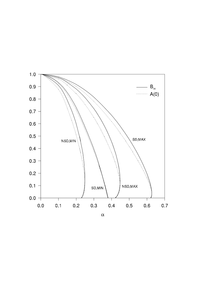
Figure 1: The metric functions $A(0)$ and $B_{m}=\mbox{min}[B(r)]$ in terms of $\alpha$.

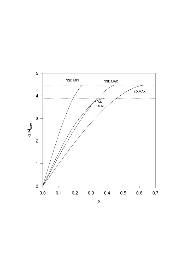
Figure 2: The ADM mass in terms of the coupling constant $\alpha$.

3.2 Minimal Symmetry Breaking Solutions

The $SU(5)$ symmetry can be broken into many minimal breaking patterns producing solutions with non-abelian stability group. In what follows, we present two types of such solutions which are invariant under the $SU(3)\times SU(2)/U(1)$ group.

First, we investigate the self-dual solution where $\Phi_{0}={\rm diag}(3,3,-2,-2,-2)$ i.e. for $b_{0}(\infty)=b_{2}(\infty)=b_{3}(\infty)=0$ and $b_{1}(\infty)=5$ while the $c_{j}$ fields satisfy the following asymptotic values $c_{0}=\frac{1}{2}$, $c_{1}=0$, $c_{2}=\frac{1}{\sqrt{3}}$ and $c_{3}=\frac{1}{\sqrt{2}}$. The corresponding solution has energy equal to $E=30$ with mass (or classical energy in the flat limit) lower compare to all types of solutions we investigated - when normalized appropriately. When it is coupled with gravity it exists up to $\alpha_{m}\approx 0.38$. Contrary to the other cases, this solution (on the main branch) bifurcates into a Reissner-Nordstrom solution with charge $Q=\sqrt{15}$ as confirmed by our numerical analysis which does not indicate the existence of a second branch. Figure 3 illustrates the way the matter functions approach their (constant) values outside the horizon (at $r=\alpha_{cr}$) of the approached Reissner-Nordstrom solution when $\alpha=0.1$ (i.e. close to the flat limit) and $\alpha=0.3797$ (i.e. close to the critical limit).

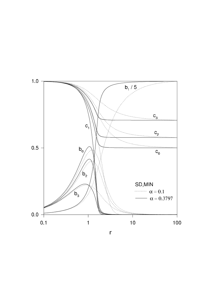
Figure 3: The matter profile functions of the self-dual minimal symmetry breaking solution for two different values of $\alpha$.

Finally, another non self-dual solution with the same unbroken group can be constructed when $\Phi_{0}$ is of the form $\Phi_{0}={\rm diag}(2,-3,2,-3,2)$ i.e. for $b_{0}(\infty)=b_{2}(\infty)=1$, $b_{1}(\infty)=b_{3}(\infty)=-1$ and $c_{j}(\infty)=0$. The corresponding mass of the configuration is equal to $M=48$.

Once more, the aforementioned solutions can be considered in the presence of gravitating fields and our numerical routines indicate that their gravitating analogues exist up to a maximal value of the coupling constant equal to $\alpha_{m}\approx 0.249$. In addition, a secondary branch exists which terminates at $\alpha\approx 0.229$ into an extremal Reissner-Nordstrom black hole of charge $Q=\sqrt{20}$. The corresponding results are presented in Figure 1 and Figure 2 (line SD, MIN) and (line NSD, MIN).

4 Conclusions

In this paper, four types of $SU(5)$ monopoles have been constructed which can be deformed by gravity forming branches of solutions labelled by the gravitational coupling constant $\alpha$. Numerical investigation of the $SU(5)$ Einstein-Yang-Mills-Higgs equations reveals that for each branch, a second one exists on the interval $\alpha\in[\alpha_{cr},\alpha_{m}$] (depending on its type) in consistence with the results obtained in smaller gauge groups like $SU(2)$ and $SU(3)$. In fact, the solution on the second branch has a higher mass than the one with the same $\alpha$ on the first (or main) branch; while, in the limit $\alpha\rightarrow\alpha_{cr}$, the minimum of the function $B(r)$ becomes deeper and deeper and approaches zero at some intermediate value $r_{h}$. Accordingly, the regular solution does not exist for $\alpha=\alpha_{cr}$ and the metric fields approach that of an extremal Reissner-Nordstrom black hole on the interval $[r_{h},\infty]$ while all matter fields tend to their asymptotic values.

Acknowledgements We gratefully acknowledge Betti Hartmann for numerous interesting discussions which turn out to be at the basis of the present work. Y.B. acknowledges the Belgian F.N.R.S. for financial support.

References

• [1] T. Ioannidou and P. M. Sutcliffe, Phys. Rev. D 60 (1999), 105009
• [2] C. P. Dokos and T. N. Tomaras, Phys. Rev. D 21 (1980), 2940
• [3] P. Breitenlohner, P. Forgacs and D. Maison, Nucl. Phys. B 383 (1992), 357; B 442 (1995), 126
• [4] T. Vachaspati, Phys. Rev. Lett. 76, 188 (1996)
• [5] N. Lepora, Monopoles and dyons in $SU(5)$ gauge unification, hep-th/0008322
• [6] L. Pogosian, D. A. Steer and T. Vachaspati, Phys. Rev. Lett. 90 (2003), 061801
• [7] Y. Brihaye, B. Hartmann, T. Ioannidou and W. Zakrzewski, Class. Quantum. Grav. 21 (2004), 517
• [8] Y. Brihaye and B. Hartmann, Phys. Rev. D 67 (2003), 044001
• [9] W. J. Zakrzewski, Low dimensional sigma models (IOP, 1989)