Heterotic Brane World

Stefan Förste, Hans Peter Nilles, Patrick Vaudrevange, Akın Wingerter

Physikalisches Institut, Universität Bonn

Nussallee 12, D-53115 Bonn, Germany

Abstract

Orbifold compactification of heterotic $\text{E}_{8}\times\text{E}_{8}^{\prime}$ string theory is a source for promising grand unified model building. It can accommodate the successful aspects of grand unification while avoiding problems like doublet-triplet splitting in the Higgs sector. Many of the phenomenological properties of the 4-dimensional effective theory find an explanation through the geometry of compact space and the location of matter and Higgs fields. These geometrical properties can be used as a guideline for realistic model building.

1 Introduction

Superstring theories are candidates for a grand unified description of all fundamental interactions. The complexity of these theories as well as our limited mathematical tools, however, makes it difficult to construct explicit models for the generalization of the (supersymmetric) standard model of particle physics. One of the major problems is a consistent and exact description of the process of compactification of six spatial dimensions from $d=10$ to $d=4$. The simplest scheme of torus compactification [1] does not allow for chiral fermions in $d=4$. More elaborate schemes such as the compactification on 6-dimensional Calabi-Yau manifolds [2] allow explicit calculations only in a limited number of cases and the road to (semi) realistic model building is still very difficult. The concept of orbifold compactification of the heterotic string [3, 4] is more successful, as it combines the simplicity of torus compactification with the presence of realistic gauge groups and particle spectra in $d=4$. The simplest orbifolds obtained by just twisting the $d=6$ torus, however, lead only to a limited number of models with usually too large gauge groups and too many families of quarks and leptons. A breakthrough towards realistic model building was achieved by the inclusion of background fields such as Wilson lines [5]. This scheme provides a mechanism for (further) gauge symmetry breakdown and, more importantly and surprisingly, an efficient way to control the number of families of quarks and leptons. It is no longer difficult to arrive at models with a 3 family structure [5] and gauge group like $\text{SU}(3)\times\text{SU}(2)\times\text{U}(1)$ [6].

In these constructions the unification of gauge coupling constants originates from the presence of a higher dimensional grand unified (GUT) gauge group (e.g. $\text{E}_{8}$ or $\text{SO}(32)$) and does not necessarily include a GUT group in $d=4$; instead only $\text{SU}(3)\times\text{SU}(2)\times\text{U}(1)$ is realized as the unbroken gauge group in four space-time dimensions. This scheme has the advantage of the appearance of incomplete representations (so-called split multiplets) with respect to the higher dimensional gauge group. Among other things this allowed an elegant solution of the notorious doublet-triplet splitting problem [6] of $\text{SU}(5)$ GUTs, where at low energy the Higgs-multiplet as a doublet of $\text{SU}(2)$ could be realized in the absence of its $\text{SU}(5)$ partner (a triplet of $\text{SU}(3)$). Recently, this mechanism has been revived [7, 8, 9, 10, 11, 12, 13] in a pure field theory language in $d=5$ and 6. This construction of so-called orbifold GUTs, however, requires a careful discussion of the consistency of the field theory description and needs a number of ad hoc assumptions. To avoid such problems, it would therefore be advisable to embed these models in the framework of consistent higher dimensional string theories.

Orbifold compactifications of the heterotic string theory are simple enough to allow for a number of explicit calculations relevant for the phenomenological properties of the scheme. This includes:

• the determination of Yukawa couplings with world sheet instanton techniques [14, 15, 16, 17, 18, 19, 20] that incorporates a new mechanism for a suppression of some of the couplings depending on the localization properties of the fields,

• the computation of threshold corrections for gauge coupling constants in view of a grand unified picture [21, 22, 23, 24],

• determination of selection rules for terms of the superpotential [25, 26] necessary for the identification of the potential flat directions and associated moduli fields.

Many of the properties of heterotic orbifolds find a nice and compelling explanation in terms of the geometrical structure of compactified space. The matter fields can either propagate in the full $d=10$ space (bulk fields in untwisted sectors) or be localized at fixed “points” of space-time dimension $d=4$ or $d=6$ (brane fields in twisted sectors). Values of Yukawa couplings, for example, depend strongly on the relative location of quark, lepton and Higgs fields. The number of generations of quarks and leptons reflects the number of compactified space dimensions [5] and/or the number of twisted sectors [27]. With these intuitive rules for model building and the potential for many explicit calculations a thorough analysis of heterotic orbifolds seems to be a promising enterprise. Early work in this direction has concentrated on the properties of the $\mathbb{Z}_{3}$ orbifold which was used as a toy model to exhibit the properties of the scheme. Some model constructions have used more general ${\mathbb{Z}}_{N}$ as well as ${\mathbb{Z}}_{N}\times{\mathbb{Z}}_{M}$ orbifolds [28], but a detailed classification of realistic models has not been reported so far [29, 30, 31, 32, 33, 34, 35, 36, 37, 38]. A pretty complete survey of these attempts can be found in [39], including a comprehensive list of references. For more recent attempts at model building see [40, 41, 42, 43, 44, 45, 46, 47, 48].

In the present paper we shall explain that a general analysis of heterotic orbifolds leads to many new results beyond those known in the framework of the ${\mathbb{Z}}_{3}$ case. It reveals a web of models with matter fields in the bulk ($d=10$), brane fields in $d=4$ (3-brane) or $d=6$ (5-brane in the usual notation) as well as intersecting 5-branes in $d=4$. This results in a multitude of models with realistic gauge groups, three families of quarks and leptons, doublet-triplet splitting and unified coupling constants. The picture of intersecting branes allows a connection with the recently much discussed field theoretic orbifold GUTs [49] and puts them in a consistent framework, in case that this is possible. In this way promising models of the bottom-up approach of field theoretic orbifold GUTs in $d=5$ or 6 could appear as lower dimensional shadows of the heterotic brane world in $d=10$. With this we also hope for a better understanding of some field theoretic results on the localization properties of bulk fields in $d=5$ and 6 [51, 52, 53] with respect to the appearance of localized tadpoles at fixed points and fixed tori along the lines of [54, 55, 56].

The present paper is devoted to an explanation of the qualitative properties of the heterotic brane world. To do this in a transparent way we shall use simple toy models and relegate the attempts at realistic model building to a future publication [58]. In section 2 we shall review the rules for constructing orbifolds with Wilson lines (the relevant technology can be found in detail in [59]). Section 3 will explain the properties of ${\mathbb{Z}}_{N}$ orbifolds (with $N$ a prime number). The toy model is based on ${\mathbb{Z}}_{3}$ and we illustrate the mechanism of gauge symmetry breakdown, and the origin of the number of families along the lines of [5, 6]. Section 4 is devoted to the analysis of ${\mathbb{Z}}_{N}\times{\mathbb{Z}}_{M}$ models. As our toy example we consider ${\mathbb{Z}}_{2}\times{\mathbb{Z}}_{2}$ . It allows the discussion of the picture of intersecting branes and offers a multitude of nontrivial patterns for the positions of matter and Higgs fields. For simplicity we restrict our discussion to a model with $\text{SO}(10)$ gauge group and 3 families of quarks and leptons. In section 5 we shall first, equipped with the brane world picture in $d=10$, zoom in on a particular pair of extra dimensions and interpret the model as an orbifold in $d=6$. This allows us to exhibit the localization of matter fields at various fixed points ($d=4$) and fixed tori (to be interpreted as bulk in the $d=6$ model). In fact, the models allow three different ways of a six dimensional interpretation which are interrelated by the consistency conditions of modular invariance of the underlying string theory. The properties of a given $d=6$ model are, of course, strongly dependent on the details of the other four compactified dimensions. Secondly, we shall analyze the breakdown of the unified gauge group in detail. In the heterotic theory in $d=10$ we start with the large gauge group $\text{E}_{8}\times\text{E}_{8}^{\prime}$. Twists and Wilson lines reduce this to a realistic gauge group $H$ in $d=4$ like $\text{SO}(10)$, $\text{SU}(5)$ or directly $\text{SU}(3)\times\text{SU}(2)\times\text{U}(1)$. Again one finds an illuminating geometrical picture of gauge symmetry breakdown. On the branes typically the unbroken gauge group is enhanced with respect to $H$, and the interplay of the various branes determines the group $H$ as the common subgroup. We exhibit this picture in detail with toy models based on the gauge group $\text{SU}(5)$ and $\text{SU}(4)\times\text{SU}(2)\times\text{SU}(2)$. Section 6 will be devoted to a discussion of the potential phenomenological properties of the heterotic brane world, including qualitative properties of gauge coupling unification, textures for Yukawa couplings, candidates for the appearance of an R-symmetry and the question of proton decay. In section 7 we shall conclude with a discussion of the strategies for explicit model building in the heterotic brane world.

2 Review of Orbifolds

We will briefly review orbifold constructions, closely following [59]. In the bosonic construction, the heterotic string is described by a 10 dimensional right moving superstring, and a 26 dimensional left moving bosonic string. We will denote the 8 right moving bosonic and fermionic coordinates of the superstring in the light-cone gauge by $X_{R}^{i}$ and $\Psi_{R}^{i}$, $i=1,\ldots,8$, respectively. The left movers include 8 bosons $X_{L}^{i}$, $i=1,\ldots,8$, and another 16 bosons $X_{L}^{I}$, $I=1,\ldots,16$, which are compactified on the torus $T_{\text{E}_{8}\times\text{E}_{8}^{\prime}}$ corresponding to the root lattice of $\text{E}_{8}\times\text{E}_{8}^{\prime}$. (The root lattice of $\text{SO}(32)$ is also an admissible choice.)

To construct a 4 dimensional string theory, 6 dimensions are compactified on a torus $T^{6}$. The resulting spectrum has $\mathcal{N}=4$ supersymmetry, and is thus non-chiral. To obtain a chiral theory with $\mathcal{N}=1$ supersymmetry, one compactifies on an orbifold [3, 4]:

$$\mathcal{O}=T^{6}\big{/}P\otimes T_{\text{E}_{8}\times\text{E}_{8}^{\prime}}\big{/}G$$ (1)

An orbifold is defined to be the quotient of a torus over a discrete set of isometries of the torus, called the point group $P$. Modular invariance requires the action of the point group to be embedded into the gauge degrees of freedom, $P\hookrightarrow G$. $G$ is in general a subgroup of the automorphisms of the $\text{E}_{8}\times\text{E}_{8}^{\prime}$ Lie algebra, and is called the gauge twisting group. In the absence of outer automorphisms, the Lie algebra automorphism can be realized as a shift $X_{L}\mapsto X_{L}+V$ in the $\text{E}_{8}\times\text{E}_{8}^{\prime}$ root lattice:

$$P\hookrightarrow G,\qquad\theta\mapsto V$$ (2)

An alternative description is to define an orbifold as

$$\mathcal{O}=\mathbb{R}^{6}\big{/}S\otimes T_{\text{E}_{8}\times\text{E}_{8}^{\prime}}\big{/}G,$$ (3)

where the lattice vectors $e_{\alpha}$, $\alpha=1,\ldots,6$, defining the 6-torus $T^{6}$ have been added to the point group to form the space group $S=\left\{\left(\theta,n_{\alpha}e_{\alpha}\right)\,\big{|}\,\,\theta\in P,\,\,\,n_{\alpha}\in\mathbb{Z}\right\}$. As before, modular invariance requires the action of the space group to be embedded into the gauge degrees of freedom,

$$S\hookrightarrow G,\qquad\left(\theta,n_{\alpha}e_{\alpha}\right)\mapsto\left(V,n_{\alpha}A_{\alpha}\right),$$ (4)

where the lattice vectors $e_{\alpha}$ are mapped to shifts $A_{\alpha}$ in the gauge lattice. The shifts $A_{\alpha}$ correspond to gauge transformations associated with the non-contractible loops given by $e_{\alpha}$, and are thus Wilson lines. The action of the orbifold group on all degrees of freedom is then given by

$$X^{i}\mapsto(\theta X)^{i}+n_{\alpha}e_{\alpha}^{i},\qquad X_{L}^{I}\mapsto X_{L}^{I}+V^{I}+n_{\alpha}A_{\alpha}^{I},$$ (5)

where $i=3,\ldots,8,$   $I=1,\ldots,16.$ Choosing complex coordinates on the torus,

$$Z^{1}=X^{3}+iX^{4},\quad Z^{2}=X^{5}+iX^{6},\quad Z^{3}=X^{7}+iX^{8},$$ (6)

the action of the point group on the space-time degrees of freedom can be neatly summarized as

$$Z^{a}\mapsto\exp\left(2\pi iv^{a}\right)Z^{a},\quad a=1,2,3,$$ (7)

where $v$ is called the twist vector.

2.1 Consistency Conditions

Different 4 dimensional models can be constructed depending on the choice of the compactification torus $T^{6}$, the point group $P$, and the embedding into the gauge degrees of freedom $P\hookrightarrow G$. There are several constraints which must be fulfilled.

The twist $\boldsymbol{\theta}$ is well-defined. To be well-defined on the compactification torus $T^{6}$, $\theta$ must be an automorphism of the torus lattice, and preserve the scalar products. In other words, $\theta$ is an isometry of the torus lattice.

$\boldsymbol{\mathcal{N}}\boldsymbol{=}\boldsymbol{1}$ supersymmetry. Acting with $\theta\in\mathbb{Z}_{N}$ on a spinor representation of SO(8), one immediately verifies that requiring $\mathcal{N}=1$ supersymmetry amounts to demanding $\pm v^{1}\pm v^{2}\pm v^{3}=0$ for one combination of signs ($v^{i}\neq 0$). In this case, one can always choose

$$v^{1}+v^{2}+v^{3}=0.$$ (8)

The generalization of these results to $\mathbb{Z}_{N}\times\mathbb{Z}_{M}$ orbifolds is given in [28]. Requiring the twist to be well-defined on the torus, and demanding $\mathcal{N}=1$ supersymmetry, it follows that $P$ must either be $\mathbb{Z}_{N}$ with $N=3,4,6,7,8,12,$ or $\mathbb{Z}_{N}\times\mathbb{Z}_{M}$ with $M,N=2,3,4,6,$ and $N$ a multiple of $M$ [3, 28]. For $N=6,8,12,$ there are 2 different choices for the point group $P$. The lattices on which $P$ acts as an isometry are the root lattices of semi-simple Lie algebras of rank 6. In some cases, there is more than one choice of lattice for a given set of symmetries $P$. (In the $\mathbb{Z}_{2}\times\mathbb{Z}_{2}$ case, the choice of the lattice in each complex dimension is arbitrary, and the complex directions are orthogonal.)

The Embedding $\boldsymbol{P}\boldsymbol{\hookrightarrow}\boldsymbol{G}$ is a group homomorphism. $\theta\in\mathbb{Z}_{N}$ implies $\theta^{N}=1\!\!1,$ which in turn implies that its embedding into the gauge degrees of freedom as a shift is the identity, i.e.

$$N\,V\in T_{\text{E}_{8}\times\text{E}_{8}^{\prime}},\quad N\,A_{\alpha}\in T_{\text{E}_{8}\times\text{E}_{8}^{\prime}}.$$ (9)

Modular invariance. For the orbifold partition function to be modular invariant, following conditions on the twist, gauge shift, and Wilson lines need to be fulfilled [59]:

$$N\left(V^{2}-v^{2}\right)=0\text{ mod }2$$

$$N\,V\cdot A_{\alpha}=0\text{ mod }1$$

$$N\,A_{\alpha}\cdot A_{\beta}=0\text{ mod }1,\quad\alpha\neq\beta$$

$$N\,A_{\alpha}^{2}=0\text{ mod }2$$ (10)

These conditions can be rewritten in a more concise form as

$$N\left[\left(mV+n_{\alpha}A_{\alpha}\right)^{2}-m^{2}v^{2}\right]=0\text{ mod }2,\quad m=0,1.$$ (11)

Modular invariance automatically guarantees the anomaly freedom of orbifold models.

For $\mathbb{Z}_{N}\times\mathbb{Z}_{M}$ orbifolds, the above conditions for modular invariance are generalized in a straightforward way. Let $v_{1}$, $v_{2}$ denote the twist vectors of $\mathbb{Z}_{N}\times\mathbb{Z}_{M}$, and $V_{1}$, $V_{2}$ the corresponding gauge shifts. Then, the first equation in eq. (10) generalizes to

$$N^{\prime}\left[\left(kV_{1}+\ell V_{2}\right)^{2}-\left(kv_{1}+\ell v_{2}\right)^{2}\right]=0\text{ mod }2,$$

$$N^{\prime}\text{ order of }kv_{1}+\ell v_{2},$$

$$k=0,\ldots,N-1,\quad\ell=0,\ldots,M-1.$$ (12)

For the Wilson lines, the conditions in eq. (10) are the same, except that they need to be fulfilled for both $V_{1}$, and $V_{2}$.

2.2 The Spectrum

On an orbifold, there are 2 types of strings, twisted and untwisted closed strings. An untwisted string is closed on the torus even before identifying points by the action of the twist:

$$X^{i}(\sigma+2\pi)=X^{i}(\sigma)+n_{\alpha}e_{\alpha}^{i},\quad i=3,\ldots,8$$ (13)

A twisted string is closed on the torus only upon imposing the point group symmetry:

$$X^{i}(\sigma+2\pi)=\left(\theta X(\sigma)\right)^{i}+n_{\alpha}e_{\alpha}^{i},\quad i=3,\ldots,8$$ (14)

From the boundary conditions, it follows that the twisted strings are localized at the points which are left fixed under the action of some element $(\theta_{i},n_{\alpha}e_{\alpha})$ of the space group $S$. These points are called the fixed points of the orbifold. We will call the element $g\equiv(\theta_{i},n_{\alpha}e_{\alpha})$ which corresponds to some given fixed point the constructing element, and denote the states which are localized at this fixed point by $\mathcal{H}_{g}$.

Since the strings propagate on the orbifold, we must project onto $S\otimes G$ invariant states. We will consider the twisted and untwisted sectors separately.

Untwisted sector. The states in the untwisted sector are those of the heterotic string compactified on a torus, where states which are not invariant under $S\otimes G$ have been projected out. The level matching condition for the massless states is given by

$$\frac{1}{2}q^{2}-\frac{1}{2}=\frac{1}{4}m_{R}^{2}=\frac{1}{4}m_{L}^{2}=\frac{1}{2}p^{2}+\tilde{N}-1=0,$$ (15)

where $q$ denotes the $\text{SO}(8)$ weight vector of the right mover ground state, e.g. $|\frac{1}{2}\,\,\frac{1}{2}\,\,\frac{1}{2}\,\,\frac{1}{2}\rangle$ or $|1\,\,0\,\,0\,\,0\rangle$. Under the action of the point group, the right and left mover states will transform as $\exp(2\pi iq\cdot v)|q\rangle_{R}$, and $\exp(2\pi ip\cdot V)|p\rangle_{L}$, respectively. Only states for which the product of these eigenvalues is 1 will survive the projection. The gauge bosons are formed by combining right movers which do not transform under the action of the point group with left movers satisfying

$$p\cdot V=0\text{ mod }1,\qquad p\cdot A_{\alpha}=0\text{ mod }1,$$ (16)

giving the unbroken gauge group. Right movers which transform non-trivially combine with left movers for which

$$p\cdot V=k/N\text{ mod }1,\quad k=1\ldots,N-1,\qquad p\cdot A_{\alpha}=0\text{ mod }1,$$ (17)

to give the charged matter. The states which include excitations for the left movers give uncharged gauge bosons (Cartan generators), the supergravity multiplet, and some number of singlets.

Twisted sectors. Without loss of generality, let us focus on the states corresponding to the constructing element $g\equiv(\theta_{i},n_{\alpha}e_{\alpha})$. The twist acts as a shift $p\mapsto p+V_{i}+n_{\alpha}A_{\alpha}$ on the momentum lattice, and as $q\mapsto q+v_{i}$ on the right mover ground state. In addition, the number operator $\tilde{N}$ is moded. The zero point energy of the right and left movers is changed by [4]

$$\delta c=\frac{1}{2}\sum_{k}\eta^{k}(1-\eta^{k}),$$ (18)

where $\eta^{k}=v_{i}^{k}\text{ mod }1$ so that $0\leq\eta^{k}<1$. The level matching condition for the massless states then reads

$$\frac{1}{2}(q+v_{i})^{2}-\frac{1}{2}+\delta c=\frac{1}{4}m_{R}^{2}=\frac{1}{4}m_{L}^{2}=\frac{1}{2}(p+V_{i}+n_{\alpha}A_{\alpha})^{2}+\tilde{N}-1+\delta c=0.$$ (19)

As compared to the untwisted sector, the projection conditions in the twisted sectors are slightly more complicated. Consider the subset $Z_{g}$ of the space group $S$ which commutes with the constructing element $g$. Acting with $Z_{g}$ on the orbifold, the Hilbert space $\mathcal{H}_{g}$ is mapped into itself. $Z_{g}$ should act as the identity on $\mathcal{H}_{g}$, thus all elements which are not invariant under $h\in Z_{g}$ are projected out.

If $h\in S$ does not commute with $g$, the action of $h$ changes the boundary conditions of the states in $\mathcal{H}_{g}$, and states in $\mathcal{H}_{g}$ will be mapped to states in $\mathcal{H}_{hgh^{-1}}$. To form invariant states, one starts with some state in $\mathcal{H}_{g}$ and considers its image in $\mathcal{H}_{hgh^{-1}}$ for all $h\in S$. In each Hilbert space, we project onto its $Z_{hgh^{-1}}$ invariant subspace. The sum of these states is then invariant under the action of the space group $S$.

3 ${\mathbb{Z}}_{N}$ Orbifolds for Prime $N$

We illustrate the discussion of the previous section by considering $\mathbb{Z}_{N}$ orbifolds with prime $N$, taking the $\mathbb{Z}_{3}$ orbifold as the paradigm.

The lattice defining the 6-torus is the $\text{SU}(3)^{3}$ root lattice as shown in figure 1. The point group $\mathbb{Z}_{3}$ is generated by $\theta$ which acts as a simultaneous rotation of 120^∘ in the three 2-tori, and in the notation of eq. (7), this corresponds to the twist vector

$$v=\frac{1}{3}\left(1,\,\,\,1,\,\,-2\right).$$ (20)

The action of $\theta$ leaves $27$ fixed points. The twisted sector corresponding to the action of $\theta^{2}$ gives the anti-particles of the aforementioned sector, so we will not consider it separately.

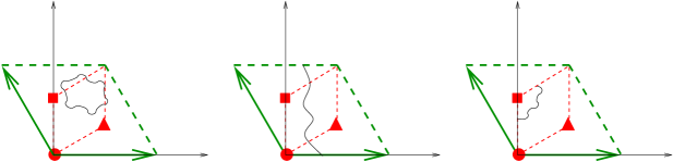
Figure 1: ${\mathbb{Z}}_{3}$ orbifold. The circle, triangle, and square denote the fixed points.

In figure 1, the strings in the first and the second torus are already closed on the torus (untwisted sector states), whereas in the third torus, the state only closes upon imposing the symmetry generated by the 120^∘ rotations (twisted sector state).

Let us first consider the untwisted sector. The action of the orbifold twist is accompanied by an action in the gauge degrees of freedom realized as a shift. We choose the standard embedding

$$V=\frac{1}{3}\left(1,\,\,\,1,\,\,-2,\,\,\,\,0^{5}\right)\left(0^{8}\right),$$ (21)

where the first 3 components of the gauge shift are equal to the components of the twist vector $v$. With this choice, the modular invariance condition eq. (10) is automatically satisfied, and the anomaly freedom of our model is guaranteed. From the 240 states in the first $\text{E}_{8}$, only 78 = 72 + 6 survive the projection condition eq. (16), and yield the charged gauge bosons of $\text{E}_{6}\times\text{SU}(3)$, whereas the second $\text{E}_{8}^{\prime}$ is left untouched.

The right mover ground state will decompose as $\boldsymbol{8}\rightarrow\boldsymbol{3}+\bar{\boldsymbol{3}}+\boldsymbol{1}+\boldsymbol{1}$ under $\text{SU}(3)\subset\text{SO}(8)$, i.e. there are 3 right mover states transforming as $|q\rangle_{R}\mapsto\exp\left(2\pi i\cdot\frac{1}{3}\right)|q\rangle_{R}$ which will combine with left movers satisfying

$$p\cdot V=\frac{2}{3}\text{ mod }1$$ (22)

to give the charged matter representations $3\times(\boldsymbol{27},\boldsymbol{3})$. From the untwisted sector, we thus get 9 families of quarks and leptons.

Let us now discuss the twisted sector, and focus on the fixed point $(\bullet,\bullet,\bullet)$ in figure 1. The shift in the zero point energy as given by eq. (18) is $\delta c=1/3$, and the level matching condition for the massless states reads

$$\frac{1}{2}(q+v)-\frac{1}{6}=\frac{1}{4}m_{R}^{2}=\frac{1}{4}m_{L}^{2}=\frac{1}{2}(p+V)^{2}+\tilde{N}-\frac{2}{3}=0.$$ (23)

The twisted right moving ground state $|q+v\rangle_{R}$ is a singlet under $\theta$. (Note that $q+v$ must be shifted by a $\text{SO}(8)$ root vector to fulfill the level matching condition). For $\tilde{N}=0$, there are 27 elements $p+V$ satisfying $(p+V)^{2}=4/3$. These left movers transform as

$$|p+V\rangle_{L}\mapsto\exp\left(2\pi i(p+V)\cdot V\right)|p+V\rangle_{L}=\exp\left(2\pi i\cdot 1\right)|p+V\rangle_{L},$$ (24)

and are invariant. They combine with the right mover to give the representation $(\boldsymbol{27},\boldsymbol{1})$. For $\tilde{N}=1/3$, there are 3 elements $p+V$ satisfying $(p+V)^{2}=2/3$. These left movers transform as

$$|p+V\rangle_{L}\mapsto\exp\left(2\pi i(p+V)\cdot V\right)|p+V\rangle_{L}=\exp\left(2\pi i\cdot\frac{2}{3}\right)|p+V\rangle_{L},$$ (25)

whereas the oscillators (one for each complex dimension) transform as

$$\tilde{\alpha}^{i}\mapsto\exp\left(2\pi i\cdot\frac{1}{3}\right)\tilde{\alpha}^{i},\quad i=1,2,3,$$ (26)

so that the states $|q\rangle_{R}\otimes\tilde{\alpha}^{i}|p\rangle_{L}$ are invariant, and give three copies of the representation $(\boldsymbol{1},\bar{\boldsymbol{3}})$. Taking into account that there are 27 fixed points, the matter content of our orbifold model is

$$3\times(\boldsymbol{27},\boldsymbol{3}),\quad 27\times(\boldsymbol{27},\boldsymbol{1}),\quad 27\times 3\times(\boldsymbol{1},\bar{\boldsymbol{3}}).$$ (27)

Thus, in the case of the standard embedding, we have 36 generations of quarks and leptons. All non-trivial embeddings of the point group into the gauge degrees of freedom have been classified [4]. For each model, we have listed the shift vector $V$, the resulting unbroken gauge group, and the number of generations in table 1.

Case	Shift $V$	Gauge Group	Gen.
1	$\left(\frac{1}{3},\frac{1}{3},\frac{2}{3},0^{5}\right)\left(0^{8}\right)$	$\text{E}_{6}\times\text{SU}(3)\times\text{E}_{8}^{\prime}$	36
2	$\left(\frac{1}{3},\frac{1}{3},\frac{2}{3},0^{5}\right)\left(\frac{1}{3},\frac{1}{3},\frac{2}{3},0^{5}\right)$	$\text{E}_{6}\times\text{SU}(3)\times\text{E}_{6}^{\prime}\times\text{SU}(3)^{\prime}$	9
3	$\left(\frac{1}{3},\frac{1}{3},0^{6}\right)\left(\frac{2}{3},0^{7}\right)$	$\text{E}_{7}\times\text{U}(1)\times\text{SO}(14)^{\prime}\times\text{U}(1)^{\prime}$	0
4	$\left(\frac{1}{3},\frac{1}{3},\frac{1}{3},\frac{1}{3},\frac{2}{3},0^{3}\right)\left(\frac{2}{3},0^{7}\right)$	$\text{SU}(9)\times\text{SO}(14)^{\prime}\times\text{U}(1)^{\prime}$	9

Table 1: Inequivalent $\mathbb{Z}_{3}$ orbifold models without Wilson lines.

Note that the proliferation of the number of generations is due to the fact that the physics at each fixed point is the same. This dramatically changes in the presence of Wilson lines [5]. We will illustrate the lifting of the degeneracy at the fixed points using a specific example. Choose the standard embedding, and the Wilson lines

$$A_{1}=A_{2}=\left(0^{6},\,\,\frac{1}{3},\,\,\frac{1}{3}\right)\left(\frac{2}{3},\,\,0^{7}\right).$$ (28)

Applying the projection conditions eq. (16), we find that the surviving gauge symmetry is

$$\text{SU}(6)\times\text{SU}(3)\times\text{U}(1)\times\text{SO}(14)^{\prime}\times\text{U}(1)^{\prime}.$$ (29)

From the untwisted sector, we obtain the charged matter representations $3\times(\boldsymbol{15},\boldsymbol{3})$. (We will only indicate the representations under the first 2 factors of the symmetry group.) Let us discuss the twisted sector in greater detail.

Consider the fixed points $(\bullet,\bullet,\bullet)$, $(\blacktriangle,\bullet,\bullet)$, and $({\scriptstyle\blacksquare},\bullet,\bullet)$ as depicted in figure 2. The fixed point $(\bullet,\bullet,\bullet)$ is left invariant under the action of $\theta$ alone, i.e. the constructing element is $(\theta,0)$. The level matching condition for massless states living at this fixed point will be the same as eq. (23). The states do not feel the presence of the Wilson lines.

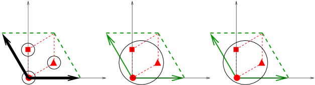
Figure 2: ${\mathbb{Z}}_{3}$ orbifold with non-vanishing Wilson lines $A_{1},A_{2}$. The circles around the fixed points indicate that the degeneracy in the first torus is lifted.

The fixed point $(\blacktriangle,\bullet,\bullet)$, however, is only invariant under the action of $\theta$ accompanied by the lattice shift $e_{1}$, and the constructing element is $(\theta,e_{1})$. The immediate consequence is that the level matching condition for the massless states changes to

$$\frac{1}{2}(q+v)-\frac{1}{6}=\frac{1}{4}m_{R}^{2}=\frac{1}{4}m_{L}^{2}=\frac{1}{2}(p+V+A_{1})^{2}+\tilde{N}-\frac{2}{3}=0.$$ (30)

Clearly, it is more difficult to fulfill the new relation, and the $\boldsymbol{27}$ of $\text{E}_{6}$ will preferentially decompose into small representations under the new gauge group. The level matching condition can only be satisfied for $\tilde{N}=0$, and these states also survive the projection condition analogous to eq. (24) (where we have to substitute $V\rightarrow V+A_{1}$) to form the representations $(\boldsymbol{1},\bar{\boldsymbol{3}})+(\bar{\boldsymbol{6}},\boldsymbol{1})$. As there are no Wilson lines in the second and third torus, the spectrum at the fixed point $(\blacktriangle,\bullet,\bullet)$ will still be 9-fold degenerate. All fixed points with $\blacktriangle$ as the first entry and an arbitrary one in the last two entries will have the same matter content. Analogous considerations also apply in the case of the fixed point $({\scriptstyle\blacksquare},\bullet,\bullet)$.

To summarize, the matter content of the model is (omitting the antiparticles)

Untwisted	$3\times(\boldsymbol{15},\boldsymbol{3})$,
$(\bullet,\cdot,\cdot)$	$9\times(\boldsymbol{15},\boldsymbol{1})$, $18\times(\bar{\boldsymbol{6}},\boldsymbol{1})$, $27\times(\boldsymbol{1},\bar{\boldsymbol{3}})$,
$(\blacktriangle,\cdot,\cdot)$	$9\times(\boldsymbol{1},\bar{\boldsymbol{3}})$, $9\times(\bar{\boldsymbol{6}},\boldsymbol{1})$,
$({\scriptstyle\blacksquare},\cdot,\cdot)$	$9\times(\boldsymbol{1},\bar{\boldsymbol{3}})$, $9\times(\bar{\boldsymbol{6}},\boldsymbol{1})$.

From the untwisted sector, we obtain 9 families, which also have $\text{SU}(3)$ quantum numbers, and from $(\bullet,\cdot,\cdot)$, we have another 9 families which are $\text{SU}(3)$ singlets. The total number of 18 families is to be compared to the 36 families in the case of no Wilson lines. Using more Wilson lines, models with 3 families of quarks and leptons [5] and with standard model gauge group $\text{SU}(3)\times\text{SU}(2)\times\text{U}(1)^{n}$ can be constructed [6].

4 ${\mathbb{Z}}_{N}\times{\mathbb{Z}}_{M}$ Orbifolds

In the previous section, we discussed ${\mathbb{Z}}_{N}$ orbifolds with $N$ being a prime number. Some additional structure arises when $N$ is not prime, or for ${\mathbb{Z}}_{N}\times{\mathbb{Z}}_{M}$ orbifolds. These theories have ${\cal N}=2$ subsectors, because the point group contains elements for which one entry of the corresponding twist vector $v$ vanishes. Actually, the fixed points under these elements are fixed tori. As the simplest example, we discuss a ${\mathbb{Z}}_{2}\times{\mathbb{Z}}_{2}$ orbifold.

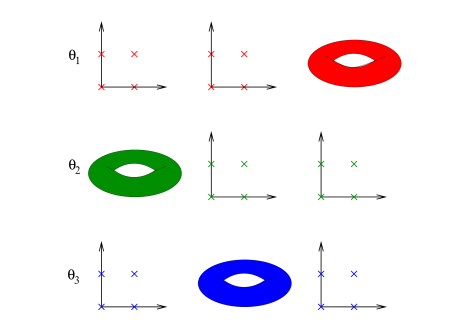
Figure 3: Action of the twists in the case of the ${\mathbb{Z}}_{2}\times{\mathbb{Z}}_{2}$ orbifold. The crosses indicate the fixed points.

4.1 ${\mathbb{Z}}_{2}\times{\mathbb{Z}}_{2}$ Orbifolds

The ${\mathbb{Z}}_{2}\times{\mathbb{Z}}_{2}$ point group consists of four elements: $1\!\!1$, $\theta_{1}$, $\theta_{2}$, and $\theta_{3}=\theta_{1}\theta_{2}$. Their action is given by rotations in three complex planes (see figure 3): $v_{1}=\left(\frac{1}{2},-\frac{1}{2},0\right)$, $v_{2}=\left(0,\frac{1}{2},-\frac{1}{2}\right)$ and $v_{3}=v_{1}+v_{2}$. Each of these twists acts only in two of the three complex planes, creating $4\cdot 4=16$ fixed points. Therefore, the strings of the twisted sectors are only fixed in four of the six compact dimensions, still free to move in two of them. Thus, the 16 fixed points of every twisted sector are in fact 16 fixed tori. Altogether, the ${\mathbb{Z}}_{2}\times{\mathbb{Z}}_{2}$ orbifold has 48 fixed tori. Counting also the $3+1$ non-compact dimensions, these are actually $5+1$ dimensional fixed planes, i.e. 5-branes. Branes belonging to different twists are mutually orthogonal, and intersect in $4d$ Minkowski space. A picture showing one brane from each twisted sector is given in figure 4. The 16 5-branes from the same twisted sector are parallel to each other.

\begin{picture}(9216.0,8658.0)(507.0,-8371.0)\end{picture}

Figure 4: Intersecting brane picture: The picture shows one brane of each twisted sector. The intersection is $4d$ Minkowski space. The branes are mutually orthogonal in the six compact dimensions.

Any of the twists break $\mathcal{N}=4$ to $\mathcal{N}=2$ supersymmetry. The combination of all twists leaves $\mathcal{N}=1$ supersymmetry unbroken.

The twists must be embedded into the gauge degrees of freedom such that

$$2\left[(kV_{1}+lV_{2})^{2}-(kv_{1}+lv_{2})^{2}\right] = 0\textmd{ mod }2,\qquad k,l=1,2$$ (31)

holds, in order to ensure modular invariance (eq. (12)). The easiest way to fulfill this condition is the standard embedding

$$V_{1} = \left(\frac{1}{2},-\frac{1}{2},0^{6}\right)\left(0^{8}\right),$$

$$V_{2} = \left(0,\frac{1}{2},-\frac{1}{2},0^{5}\right)\left(0^{8}\right),$$

$$V_{3} = V_{1}+V_{2}.$$

The untwisted sector is given by the spectrum of the heterotic string, projected onto $S\otimes G$ invariant states. These states are now sorted with respect to their eigenvalues. The eigenvalues for right and left movers are given by

$$\exp(2\pi iq\cdot v_{i})|q\rangle_{R} \exp(2\pi ip\cdot V_{i})|p\rangle_{L},$$ and (32)

for $i=1,2,3$, and only invariant combinations of right and left movers survive. The $\text{E}_{8}\times\text{E}_{8}^{\prime}$ gauge group of the heterotic string breaks to $\text{E}_{6}\times\text{U}(1)^{2}\times\text{E}_{8}^{\prime}$. The remaining 168 roots of the broken $\text{E}_{8}\times\text{E}_{8}^{\prime}$ become matter states

$3\times\boldsymbol{27}$, $3\times\boldsymbol{\overline{27}}$ and $6\times\boldsymbol{1}$.

In the twisted sector the mass formula for the left movers changes (see eq. (19)), because of the change in the zero point energy and because of the shifted root lattice $p_{\textmd{sh}}=p+V_{i}$

$$\frac{(p+V_{i})^{2}}{2}+\tilde{N}-\frac{3}{4} = 0.$$ (33)

Each constructing element of the space group corresponds to two different mass formulas: one with (moded) excitations for the left movers and one without excitations. We give an example

$$(\theta_{2},e_{3})\Rightarrow\begin{cases}(p+V_{2})^{2}=\frac{3}{2}&\quad\text{for }\tilde{N}=0\\ (p+V_{2})^{2}=\frac{1}{2}&\quad\text{for }\tilde{N}=\frac{1}{2},\end{cases}$$ (34)

where $p$ is an element of the $\text{E}_{8}\times\text{E}_{8}^{\prime}$ lattice. Here, the torus shift $e_{3}$ of the constructing element does not play a role for the mass formulas. In the presence of Wilson lines this will change.

Taking a closer look at the mass formulas, one can see that the equation for $\tilde{N}=0$ allows a wide range of choices for the root vector $p$, leading to quite large representations. Compared to this the equation for $\tilde{N}=\frac{1}{2}$ is much more restrictive and will mostly lead to singlets.

Case	Shifts	Gauge Group	Gen.
1	$\left(\frac{1}{2},-\frac{1}{2},0^{6}\right)\left(0^{8}\right)$ $\left(0,\frac{1}{2},-\frac{1}{2},0^{5}\right)\left(0^{8}\right)$	$\text{E}_{6}\times\text{U}(1)^{2}\times\text{E}_{8}^{\prime}$	48
2	$\left(\frac{1}{2},-\frac{1}{2},0^{6}\right)\left(0^{8}\right)$ $\left(0,\frac{1}{2},-\frac{1}{2},0^{4},1\right)\left(1,0^{7}\right)$	$\text{E}_{6}\times\text{U}(1)^{2}\times\text{SO}(16)^{\prime}$	16
3	$\left(\frac{1}{2}^{2},0^{6}\right)\left(0^{8}\right)$ $\left(\frac{5}{4},\frac{1}{4}^{7}\right)\left(\frac{1}{2},\frac{1}{2},0^{6}\right)$	$\text{SU}(8)\times\text{U}(1)\times\text{E}_{7}^{\prime}\times\text{SU}(2)^{\prime}$	16
4	$\left(\frac{1}{2}^{2},0^{5},1\right)\left(1,0^{7}\right)$ $\left(0,\frac{1}{2},-\frac{1}{2},0^{5}\right)\left(-\frac{1}{2},\frac{1}{2}^{3},1,0^{3}\right)$	$\text{E}_{6}\times\text{U}(1)^{2}\times\text{SO}(8)^{\prime 2}$	0
5	$\left(\frac{1}{2},-\frac{1}{2},-1,0^{5}\right)\left(1,0^{7}\right)$ $\left(\frac{5}{4},\frac{1}{4}^{7}\right)\left(\frac{1}{2},\frac{1}{2},0^{6}\right)$	$\text{SU}(8)\times\text{U}(1)\times\text{SO}(12)^{\prime}\times\text{SU}(2)^{\prime 2}$	0

Table 2: Classification of ${\mathbb{Z}}_{2}\times{\mathbb{Z}}_{2}$ orbifolds without background fields.

As described in section 2.2 the right movers also become twisted. As in the untwisted case, right and left movers now have to be sorted with respect to their eigenvalues under all shifts. It is important to notice that all left movers (of the untwisted sector and of the twisted sectors) find a right moving partner to form invariant states. Since the states of the twisted sectors are half-hypermultiplets of $\mathcal{N}=2$ supersymmetry, CP conjugation is needed to form complete $\mathcal{N}=1$ chiral multiplets. The eigenvalue of the chirality is defined as the first entry of the right moving $\text{SO}(8)$ spinor (Ramond state). We choose to count states with negative chirality and combine them with their CP partners to get complete multiplets. A CP partner is equal to the original state except for a multiplication with $-1$ in the $\text{E}_{8}\times\text{E}_{8}^{\prime}$ root lattice of the left mover and in the $\textmd{SO}(8)$ lattice of the right mover. Therefore also the eigenvalues of the left and right mover are the same except for a multiplication with $-1$. Using this in case of the standard embedding the matter content of the twisted sector is

$48\times\boldsymbol{27}$ and $240\times\boldsymbol{1}$,

where five singlets and one $\boldsymbol{27}$ live on every fixed torus. Since the untwisted sector has a net number of zero families, the standard embedding leads to a chiral spectrum with a net number of 48 families.

We have classified all ${\mathbb{Z}}_{2}\times{\mathbb{Z}}_{2}$ orbifold models without background fields. It turns out that there are only five inequivalent combinations of shifts. We present the result in table 2. The first model (standard embedding) has already been presented in [28].

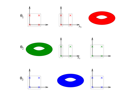
Figure 5: Wilson line in $e_{3}$ direction lifts the degeneracy of the fixed points as indicated by the boxes.

4.2 Adding Wilson Lines

Wilson lines are needed to get interesting gauge groups and to reduce the number of families. As explained in section 2, Wilson lines are the embedding of the torus shifts into the gauge degrees of freedom. In the untwisted sector, states with left movers that are invariant under their action survive, i.e.

$$p\cdot A_{i} \in {\mathbb{Z}},$$

and the other states are projected out. Therefore, they break the gauge group. Additionally, Wilson lines control the number of families in the twisted sectors. This is due to the fact that Wilson lines can distinguish between different fixed points by changing the mass formulas. For example, without Wilson lines the constructing elements $(\theta_{2},0)$ and $(\theta_{2},e_{3})$ lead to the same mass formulas. This changes now:

$$(\theta_{2},0) \Rightarrow \begin{cases}(p+V_{2})^{2}=\frac{3}{2}&\quad\text{for }\tilde{N}=0\\ (p+V_{2})^{2}=\frac{1}{2}&\quad\text{for }\tilde{N}=\frac{1}{2}\end{cases}$$ (35)

$$(\theta_{2},e_{3}) \Rightarrow \begin{cases}(p+V_{2}+A_{3})^{2}=\frac{3}{2}&\quad\text{for }\tilde{N}=0\\ (p+V_{2}+A_{3})^{2}=\frac{1}{2}&\quad\text{for }\tilde{N}=\frac{1}{2}\end{cases}$$ (36)

We illustrate the lifting of the degeneracy of the fixed points in figure 5.

The $\tilde{N}=\frac{1}{2}$ mass equation in the $(\theta_{2},e_{3})$ case is too restrictive to give any other representations but singlets. But by a clever choice of Wilson lines, the $\tilde{N}=0$ mass equation for the same fixed point still allows both: either to have a representation of a family or several smaller ones. Hence, Wilson lines reduce the number of families.

A second way in which Wilson lines control the number of families appears only in presence of fixed tori. A Wilson line that corresponds to a direction in a fixed torus acts like an additional projector. This is due to the fact that one has to project onto all elements of $Z_{g}$, which is the set of space group elements that commute with the constructing element $g$ (section 2.2). We give an example. Suppose that $g=(\theta_{3},e_{1})$ is the constructing element. Then the set of commuting space group elements $Z_{g}$ consists of several elements, e.g. the constructing element $g$ itself and $(\theta_{2},e_{3})$

$$\left[(\theta_{3},e_{1}),(\theta_{2},e_{3})\right]=0\text{ .}$$ (37)

Thus one has to calculate the eigenvalues with respect to all elements of $Z_{g}$ for the left and right movers. We show how to calculate the eigenvalues for the commuting element $(\theta_{2},e_{3})$

$$\exp\left(2\pi ip_{\textmd{sh}}\cdot(V_{2}+A_{3})\right)|p_{\textmd{sh}}\rangle_{L}\quad \quad\exp\left(2\pi iq_{\textmd{tw}}\cdot v_{2}\right)|q_{\textmd{tw}}\rangle_{R}$$ and (38)

where $p_{\textmd{sh}}=p+V_{3}+A_{1}$ and $q_{\textmd{tw}}=q+v_{3}$ correspond to the constructing element $(\theta_{3},e_{1})$. Only invariant combinations of right and left movers survive the projection. It is important to notice that due to these additional projections in the presence of Wilson lines, not all left movers find a right moving partner to form invariant states.

4.3 SO(10) Model with Three Families

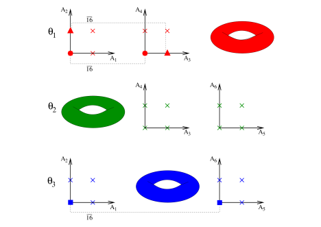
Figure 6: Localization of the families for the toy $\text{SO}(10)$ model.

Wilson lines are therefore a promising tool to construct interesting models. As a toy model, we present an $\text{SO}(10)$ model with three families. We use standard embedding together with the six Wilson lines

$A_{1}=(0^{7},1)(1,0^{7})$,	$A_{4}=(0^{8})(1,0^{3},\frac{1}{2},-\frac{1}{2},\frac{1}{2},\frac{1}{2})$,
$A_{2}=(0^{8})(0,1,\left(\frac{1}{2}\right)^{4},0^{2})$,	$A_{5}=(0^{8})(0,\frac{1}{2},-1,\frac{1}{2},-\frac{1}{2},0,\frac{1}{2},0)$,
$A_{3}=(0^{8})(0^{2},\frac{1}{2},-\frac{1}{2},-\frac{1}{2},\frac{1}{2},-1,0)$,	$A_{6}=(0^{8})(1,0^{3},\frac{1}{2},-\frac{1}{2},\frac{1}{2},\frac{1}{2})$.

The first half of $A_{1}$ breaks $\text{E}_{6}\times\text{U}(1)^{2}$ to $\text{SO}(10)\times\text{U}(1)^{3}$. The other Wilson lines do not break this any further. The hidden $\text{E}_{8}^{\prime}$ breaks to $\text{U}(1)^{\prime 8}$. The matter content is

untwisted sector:	$12\times\boldsymbol{1}$ and $6\times\boldsymbol{10}$
twisted sector:	$174\times\boldsymbol{1}$, $3\times\boldsymbol{\overline{16}}$ and $5\times\boldsymbol{10}$.

The $\boldsymbol{\overline{16}}$ of $\text{SO}(10)$ counts as a family, thus we have a three family toy model of $\text{SO}(10)$. Their localization is illustrated in figure 6. The two families of the $\theta_{1}$ sector live on parallel 5-branes and the third family of the $\theta_{3}$ sector lives on an orthogonal brane. Interestingly, not every twisted sector leads to a family. Matter in non-trivial representations under $\text{SO}(10)$ is listed in table 3.

sector	# of $\boldsymbol{10}$s	# of $\boldsymbol{\overline{16}}$s
untwisted	6	0
$(\theta_{1},0)$	1	1
$(\theta_{1},e_{2}+e_{3})$	1	1
$(\theta_{2},0)$	1	0
$(\theta_{2},e_{4}+e_{6})$	1	0
$(\theta_{3},0)$	1	1
sum	11	3

Table 3: $\text{SO}(10)$ model. Matter states in non-trivial representations.

5 Exploiting the Geometric Picture

One advantage of orbifold compactifications is that they provide a clear geometric picture. String theory predicts whether certain fields are constrained to live on a lower dimensional brane or can propagate through the bulk in a very simple way: Twisted sector states are constrained to the corresponding fixed plane, whereas untwisted fields propagate in ten space-time dimensions. In particular, the gauge fields are always bulk fields in heterotic models. Matter fields can come from untwisted as well as twisted sectors and hence can be bulk as well as brane fields. In the following we are going to exploit the geometric picture for our ${\mathbb{Z}}_{2}\times{\mathbb{Z}}_{2}$ example further.

5.1 Localization of Charged Matter

Here, we discuss the localization of charged matter in a setting where we zoom in on one of the compact two-tori. Physically this would correspond to a situation in which two of the extra dimensions are larger than the other four. We should stress, however, that we will not discuss the size of the extra dimensions here but merely want to give a detailed geometric picture of our example.

To this end let us zoom in on the first torus. First, we restrict our discussion to the three families transforming in the $\boldsymbol{\overline{16}}$ of SO(10). The families appear in the $\theta_{1}$ and $\theta_{3}$ twisted sector and are localized at fixed points in the first torus: There is one family at the $\left(\theta_{1},0\right)$ fixed point and one at the $\left(\theta_{3},0\right)$ fixed point. In the zoomed in picture these families are both localized at the origin in the first torus lattice. A third family lives at the $\left(\theta_{1},e_{2}+e_{3}\right)$ fixed point which corresponds to the point $e_{2}/2$ in the first torus. The distribution of the families within the first torus is shown in figure 7.

For the discussion of Yukawa couplings (see next section) it is also important where Higgs fields appear in the compact geometry. In our toy model we do have several fields transforming in the $\boldsymbol{10}$ of SO(10), i.e. many candidates for a standard model Higgs field. The localization of these $\boldsymbol{10}$s within the first torus is as follows: In the bulk there are eight fields, six from the untwisted sector and two from the $\theta_{2}$ twisted sector, since the first torus is invariant under $\theta_{2}$. Further, there are two $\boldsymbol{10}$s at the origin: one from the $\theta_{1}$ twisted sector and one from the $\theta_{3}$ twisted sector. Another $\boldsymbol{10}$ from the $\theta_{1}$ twisted sector sits at the point $e_{2}/2$.

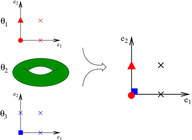
Figure 7: In this picture we focus on the localization of families within the first torus. The left hand side shows the three twisted sectors separately, whereas on the right hand side they are merged into one representation. For the sake of clarity we do not show the 11 Higgs candidates. Their localization is given in the text.

If we zoom in on the second torus, the family from the $\theta_{3}$ twisted sector lives in the bulk. Out of the families from the $\theta_{1}$ twisted sector, one lives at the origin of the second torus and one at the fixed point $e_{3}/2$. The family localization is summarized in figure 8. Furthermore, there are seven $\boldsymbol{10}$s in the bulk (six from the untwisted and one from the $\theta_{3}$ twisted sector). From the $\theta_{1}$ twisted sector one gets one $\boldsymbol{10}$ at the origin and one $\boldsymbol{10}$ at $e_{3}/2$. One $\boldsymbol{10}$ from the $\theta_{2}$ twisted sector is localized at the origin and one at $e_{4}/2$.

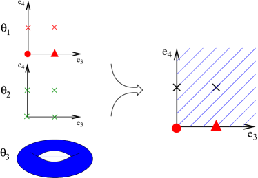
Figure 8: The family localization within the second torus is shown. The diagonal lines symbolize one family living in the bulk. (For more explanations, see figure 7.)

Finally, zooming in on the third torus provides a setup where two families (from the $\theta_{1}$ twisted sector) live in the bulk of the third torus, whereas the family from the $\theta_{3}$ twisted sector is localized at the origin. The $\boldsymbol{10}$s are distributed as follows: eight in the bulk (from untwisted and $\theta_{1}$ twisted sectors), two at the origin (from the $\theta_{2}$ and $\theta_{3}$ twisted sector), and one at $e_{6}/2$ (from the $\theta_{2}$ twisted sector). Figure 9 shows how the families are localized within the third torus.

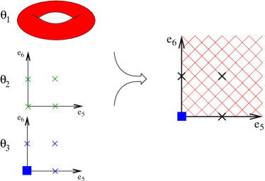
Figure 9: The family localization within the third torus is shown. The diagonal lines symbolize two families living in the bulk. (For more explanations, see figure 7.)

5.2 Gauge Group Geography

In this subsection we are going to provide a picture of the local physics at the fixed points. Such a description was used in [54] to develop the concept of fixed point equivalent models. Fixed point equivalent models yield the same spectrum at a given fixed point. Since they are usually chosen to have a simpler structure (no Wilson lines), they are very helpful for answering questions concerning the local physics at a fixed point. The picture we will present is also useful in order to make contact with the so called orbifold GUTs. Orbifold GUTs are field theoretic descriptions where one compactifies a higher dimensional field theory on an orbifold. The transformation properties of the fields under the orbifold group are usually given by assigning parities to the fields by hand. In addition, localized matter is also added by hand. (For a review see [49].) In string theory, all these data are dictated e.g. by modular invariance which automatically ensures anomaly free theories in the higher dimensions as well as in four space-time dimensions.

Since the orbifold fixed planes in our model are five-branes, it is natural to discuss a six dimensional orbifold GUT picture. If we choose for example the first torus to represent the extra dimensions of a 6d orbifold GUT, we would first compactify the heterotic string on a $T^{4}/{\mathbb{Z}}_{2}$ where the ${\mathbb{Z}}_{2}$ twist is given by $\theta_{2}$. The resulting spectrum is the bulk spectrum of the orbifold GUT. In a second step, this six dimensional theory is compactified on a $T^{2}/{\mathbb{Z}}_{2}$ where the ${\mathbb{Z}}_{2}$ is generated by $\theta_{1}$. Due to the presence of Wilson lines we have different projection conditions on different fixed points. In [13, 62] such a situation is viewed as a $T^{2}/{\mathbb{Z}}_{2}\times{\mathbb{Z}}_{2}\times{\mathbb{Z}}_{2}$ orbifold. Since we know how the space group elements containing $\theta_{1}$ act on the string states, all the parities are given by our initial choice of the heterotic orbifold. In addition, we also know which fields to localize on the fixed points from our analysis of the twisted sectors.

Just in order to show, that it is not so difficult to find more three generation models in ${\mathbb{Z}}_{2}\times{\mathbb{Z}}_{2}$ orbifolds we are going to illustrate the above discussion at the example of a three generation $\text{SU}(5)$ model. Let us first briefly present this model leaving out many details (which will be given elsewhere). The orbifold shift is again standard embedded, and there are five Wilson lines along the first five directions in $T^{2}\times T^{2}\times T^{2}$:

$A_{1}=$ $\left(0^{6},\frac{1}{2},\frac{1}{2}\right)$ $\left(1,\frac{1}{2},\frac{1}{2},0^{5}\right)$,	$A_{2}=$ $\left(\frac{1}{2},\frac{1}{2},\frac{1}{2},0^{3},\frac{1}{2},0\right)$ $\left(1,-\frac{1}{2},0,\frac{3}{2},\frac{1}{2},\frac{1}{2},1,0\right)$,
$A_{3}=$ $\left(0^{8}\right)$ $\left(1,1,-1,0,\frac{1}{2},-\frac{1}{2},\frac{1}{2},-\frac{3}{2}\right)$,	$A_{4}=$ $\left(0^{6},\frac{1}{2},\frac{1}{2}\right)$ $\left(\frac{1}{2},0^{2},-\frac{1}{2},0^{3},1\right)$,
$A_{5}=$ $\left(0^{8}\right)$ $\left(1,1,-1,0,\frac{1}{2},-\frac{1}{2},\frac{1}{2},-\frac{3}{2}\right)$.

The four dimensional gauge group is $\text{SU}(5)$ times $\text{U}(1)$ factors. One family contains a $\boldsymbol{5}$ and a $\boldsymbol{\overline{10}}$. In the untwisted spectrum there are three $\boldsymbol{5}$s and three $\boldsymbol{\overline{5}}$s giving a net number of zero families. The three families arise from various twisted sectors. The relevant matter is listed in table 4.

twist sector	# of 5s	# of $\boldsymbol{\overline{5}}$s	# of 10s	# of $\boldsymbol{\overline{10}}$s
$(\theta_{1},0)$	2	1	0	1
$(\theta_{1},e_{1})$	2	0	0	0
$(\theta_{1},e_{3}+e_{4})$	2	0	0	0
$(\theta_{2},0)$	0	1	0	0
$(\theta_{2},e_{3}+e_{5})$	0	1	0	0
$(\theta_{2},e_{6})$	0	1	0	0
$(\theta_{2},e_{3}+e_{5}+e_{6})$	0	1	0	0
$(\theta_{3},0)$	0	1	0	1
$(\theta_{3},e_{1})$	2	0	0	0
$(\theta_{3},e_{6})$	0	1	0	1
$(\theta_{3},e_{1}+e_{6})$	2	0	0	0
sum	10	7	0	3

Table 4: $\text{SU}(5)$ model. Twisted sector states in non-trivial representations.

Further details of this model will be discussed in a forthcoming publication.

Here, we restrict our attention to the interpretation as a six dimensional field theory orbifold. We choose the first torus to be the one playing the role of the extra dimensions in the field theory orbifold. Let us first focus on the pattern of gauge symmetry breaking. In the bulk of that orbifold we have the gauge group SO(12)$\times$SU(2)$\times$SU(2). This comes from applying the projection conditions arising from $\theta_{2}$ and the Wilson lines $A_{3},A_{4},A_{5}$ on the E${}_{8}\times$E₈ gauge group. The remaining orbifold elements relate the value of the gauge field at a point of the first torus to its value at the image point. For a fixed point it imposes a projection condition reducing the size of the gauge group. For example imposing invariance under $(\theta_{1},0)$ reduces SO(12)$\times$SU(2)$\times$SU(2) to SU(6)$\times$SU(2). At the fixed point $e_{1}/2$ we have to impose invariance under $(\theta_{1},e_{1})$. In the first E₈, the first Wilson line and the fourth Wilson line are the same. Hence on the bulk gauge group, $(\theta_{1},e_{1})$ acts in the same way as $(\theta_{1},0)$, and the bulk symmetry is broken to the same SU(6)$\times$SU(2). At the fixed point $e_{2}/2$, however, the bulk symmetry is reduced to SO(10) (by imposing invariance under $(\theta_{1},e_{2})$). The same happens at $(e_{1}+e_{2})/2$. The situation is illustrated in figure 10.

Figure 10: 6d field theory orbifold picture of gauge symmetry breaking pattern in the SU(5) model. In the bulk there is an SO(12)$\times$SU(2)$\times$SU(2) gauge group. Gauge groups written at lines connecting two fixed points are the ones surviving both of the corresponding projection conditions.

Massless gauge fields in four dimensions arise from 6d gauge field configurations not depending on the extra coordinates. This is possible only if the gauge field lies in the overlap of the gauge groups surviving all projection conditions. In our case this leads to an SU(5) symmetry in four dimensions. The matter from the $\theta_{2}$ twisted sectors lives in the bulk of the torus, whereas the matter from the other twisted sectors is localized at the corresponding fixed points.

As a second example we want to discuss a model with Pati–Salam gauge group $\text{SU}(4)\times\text{SU}(2)\times\text{SU}(2)$. (We suppress the hidden sector gauge group and U(1) factors. The rank of the gauge group is never reduced in our models.) Again, this is obtained from the standard embedding and five additional Wilson lines:

$A_{1}=$ $(0^{4},\frac{1}{2},\frac{1}{2},0^{2})$ $(\frac{1}{2},\frac{1}{2},1,0^{5})$,	$A_{2}=$ $(0^{6},\frac{1}{2},\frac{1}{2})$ $(0^{3},\frac{1}{2},\frac{1}{2},1,0^{2})$,
$A_{3}=$ $(0^{8})$ $(\frac{1}{2},-\frac{1}{2},1,0^{3},\frac{1}{2},\frac{1}{2})$,	$A_{4}=$ $(0^{8})$ $(0^{2},-1,\frac{1}{2},-\frac{1}{2},0,\frac{1}{2},-\frac{1}{2})$,
$A_{5}=$ $(0^{8})$ $(\frac{1}{2},-\frac{1}{2},1,0^{3},\frac{1}{2},\frac{1}{2})$.

As generations we count the $(\boldsymbol{4},\boldsymbol{2},\boldsymbol{1})$ representation of the Pati–Salam group. We focus our discussion only on this representation, leaving out matter transforming differently. (Equivalently we could count $(\boldsymbol{\overline{4}},\boldsymbol{1},\boldsymbol{2})$ since these representations come always together in the considered model.) There is one generation at the $(\theta_{1},0)$ fixed point, one generation at the $(\theta_{3},0)$ fixed point and one generation at the $(\theta_{3},e_{6})$ fixed point.

For the interpretation as a 6d orbifold we take again the first torus as the one with the extra field theory dimensions. The Wilson lines in the second and third tori have entries only in the (hidden sector) second E₈. So, the gauge group in the bulk is E${}_{7}\times$SU(2) in the observable sector. Here, it appears that the reduced gauge group at different fixed points is the same (e.g. E₆), which however can be embedded differently into the bulk gauge group. Therefore, in figure 11 gauge groups written at lines connecting the fixed points can be smaller than the gauge groups at the fixed points. In this model all three generations are located at the origin of the torus.

Figure 11: 6d field theory orbifold picture of gauge symmetry breaking pattern in the model with Pati–Salam gauge group. In the bulk there is an E${}_{7}\times$SU(2). The groups written at the lines are the common overlap of the reduced gauge groups appearing at the fixed points connected by the line.

We have seen that orbifold GUTs are incorporated into heterotic orbifolds in a very natural way. Consistency is guaranteed due to the underlying consistent string theory. A similar discussion can be found in [50] where a ${\mathbb{Z}}_{6}={\mathbb{Z}}_{3}\times{\mathbb{Z}}_{2}$ model with unbroken Pati-Salam group is presented. These authors derived a five dimensional field theory orbifold from a heterotic model. This, of course, can also be done in a straightforward way in our model. Indeed, in the ${\mathbb{Z}}_{2}\times{\mathbb{Z}}_{2}$ model one has the maximal freedom in choosing the radii. Finally, we would like to point out that knowledge about the gauge group geography is also relevant for conceptual questions like local anomaly cancellation [51, 52, 53, 54, 55, 56].

6 Towards Realistic Models

So far we have discussed just a few simple models to illustrate properties of the heterotic brane world. The conditions outlined in section 2 have been meanwhile incorporated in computer programs that allow the efficient and fast construction of many new models, in fact, many more as we are able to classify. Of course, we are primarily interested in the construction of realistic models that contain the standard model of particle physics and we have to develop a strategy to select interesting models guided by phenomenological requirements.

Especially in the framework of the ${\mathbb{Z}}_{N}\times{\mathbb{Z}}_{M}$ picture we expect a multitude of promising models. In this paper, however, we shall not focus on explicit discussion of such models and refer the reader to an upcoming publication [58]. Instead we shall discuss the properties of the heterotic brane world models at the qualitative level to point out which phenomenological questions can be addressed successfully within this picture.

6.1 Phenomenological Restrictions

The questions we hope to answer in this scheme will be concerned with

Gauge coupling unification. With this we mean an explanation of the values of the gauge couplings of $\text{SU}(3)\times\text{SU}(2)\times\text{U}(1)$ from the string coupling constant. Note that this does not necessarily require the notion of a grand unified group in $d=4$. Still we would like to understand the correct value of $\sin^{2}\Theta_{W}$ as well as possible threshold corrections. For an earlier discussion see [63].

Yukawa coupling unification. As in the case of the gauge couplings we would like to link the values of Yukawa couplings to the unified string coupling. We should try to see whether a given model allows for a parameterization of the correct pattern of quark and lepton masses as well as mixing angles. In particular, we would like to identify the explanation of a suppression mechanism for some of the couplings as the origin for the hierarchy of quark and lepton masses. This analysis will include a calculation of world sheet instanton contribution to the effective superpotential. In the past such a discussion has been given in [64, 65, 66, 67]. For more recent discussion see [68, 69, 70]. We expect a geometrical explanation of such a pattern in the heterotic brane world picture.

Baryon- and lepton-number violation. Typically we have to worry about the stability of the proton. Can we hope for a (discrete) symmetry like R-parity to avoid problems with proton decay?

Gauge hierarchy problem. Why is the weak scale so small compared to the string scale? We will assume the presence of ${\cal N}=1$ supersymmetry in $d=4$. But even then we have to solve the doublet-triplet splitting problem (hopefully through split multiplets as in [6]) and the so-called $\mu$ problem, with $\mu$ being the mass parameter in the Higgs superpotential. Is there a connection with axions as a solution to the strong CP-problem [71]? Supersymmetry has to be broken at a scale small compared to the string scale. Can we create a hidden sector responsible for that breakdown [72, 73, 74, 75], as e.g. the $\text{E}_{8}^{\prime}$ sector of the heterotic $\text{E}_{8}\times\text{E}_{8}^{\prime}$ theory?

Gauge symmetry breakdown. This question might be relevant at several stages; e.g. the breakdown of a grand unified group, or the breakdown of weak interaction $\text{SU}(2)\times\text{U}(1)$. Often, the rank reduction of the underlying gauge group needs a specific mechanism [76, 25], which very often boils down to the breakdown of additional $\text{U}(1)$ gauge bosons.

There are, of course, more detailed questions to be asked for realistic model building (absence of flavour changing neutral currents, origin of CP-violation just to name a few) that acquire the knowledge of very specific properties of the models under consideration. In our discussion here we shall, however, first concentrate on the more qualitative issues quoted above in the framework of a geometrical picture.

6.2 Properties of Heterotic Orbifolds

So let us now inspect key properties of heterotic brane world models in view of the phenomenological applications.

Gauge group. It is a subgroup of $\text{E}_{8}\times\text{E}_{8}^{\prime}$ or $\text{SO}(32)$. We concentrate here on $\text{E}_{8}\times\text{E}_{8}^{\prime}$ as this theory is phenomenologically preferable. These groups lead to chiral fermions in $d=10$ but not in $d=4$. Thus we need a subgroup that allows for parity violation in $d=4$. This could be a grand unified theory like the $\text{SO}(10)$ and $\text{SU}(5)$ toy examples given in the earlier sections, smaller groups like $\text{SU}(4)\times\text{SU}(2)\,{\mbox{and}}\,\text{SU}(3)^{3}$ or just the standard model gauge group $\text{SU}(3)\times\text{SU}(2)\times\text{U}(1)$. The latter would be preferable since it allows the presence of split multiplets [6] and in addition we do not need to incorporate the Higgs multiplets for the spontaneous breakdown of the grand unified gauge group. In fact, it turns out to be practically impossible to obtain the necessary representations in the framework of realistic $\text{SO}(10)$ and $\text{SU}(5)$ models [77]. In the intermediate cases (like Pati-Salam group or $\text{SU}(3)^{3}$ trinification [43]) such Higgs fields could be present as they originate from a (split) 27-dimensional representation of an underlying $\text{E}_{6}$. At this point we should mention a weakness of the construction explained in this paper. It does not allow the reduction of the rank of the gauge group. This is the price we have to pay for the simplicity of the construction. Thus if we start with $\text{E}_{8}\supset\text{SU}(3)\times\text{SU}(2)\times\text{U}(1)$ we will have four additional $\text{U}(1)$ factors. Rank reduction needs more input, as e.g. the implementation of continuous Wilson lines [76] or the consideration of so-called degenerate orbifolds [25]. We shall not discuss this here in detail. So let us now consider a theory with standard model gauge group in $d=4$. Although this is not a bona fide GUT model in $d=4$ it might inherit a lot of the successful properties of e.g. the $\text{SO}(10)$ or $\text{E}_{6}$ theory. A family of quarks and leptons is in the 16-dimensional representation of $\text{SO}(10)$ which also contains an R-symmetry that forbids fast proton decay by dimension 4 operators in the supersymmetric framework. These are remnants of the underlying grand unified group in $d>4$ such as $\text{SU}(5)\subset\text{SO}(10)\subset\text{E}_{6}\subset\text{E}_{7}\subset\text{E}_{8}$. Even better, some of the problems of GUTs (such as the doublet-triplet splitting problem) are solved because Higgs bosons (as well as gauge bosons) appear in incomplete (split) multiplets. Many of the phenomenological properties of the $d=4$ theory will depend on the degree to which it remembers its grand unified origin in $d>5$. This includes the value of $\sin^{2}\Theta_{W}$, the question of proton stability and the unification of Yukawa couplings. To understand these remnants of higher dimensional grand unification it is extremely useful to examine the geography of gauge group realizations like those shown in figure 10 and 11 for the example under consideration. In connection with the knowledge of the localization of matter and Higgs fields we can read off allowed and forbidden couplings, as Yukawa interactions and B, L violating operators. At the various locations, gauge groups are typically enhanced with respect to $\text{SU}(3)\times\text{SU}(2)\times\text{U}(1)$ and this might forbid unwanted operators and couplings. As we shall see in [58] these properties will prove to be useful for realistic model building.

Spectrum of matter and Higgs fields. One would aim at the constructions of models with 3 net families of quarks and leptons. This is certainly true for models with standard model gauge group. At an intermediate step, however, one might also consider models with a grand unified group and a different number of matter families. The reason for this comes from the fact that in our approach with quantized Wilson lines a gauge symmetry breakdown is usually accompanied by a change in the number of families. If we consider, for example, our $\text{SO}(10)$ model from section 4 (with 3 families) and consider another Wilson line to break the gauge symmetry we would then obtain the wrong number of families. In that sense some other $\text{SO}(10)$ model with a different number of families would represent the underlying grand unified picture of a 3 family standard model. Another point to stress is the possible presence of anti-generations. In fact, models with just 3 generations usually give only limited flexibility to accommodate a realistic pattern of Yukawa couplings. Therefore, it might be advisable to search for models with $n>3$ families and $n-3$ anti-families as well. Very often, the number of families is connected to the geometrical properties of the model. In the early construction of the $\mathbb{Z}_{3}$ orbifold families could be obtained in the untwisted sector and the number 3 found its explanation in the number of complex compactified dimensions [5]. In other cases a factor 3 appeared because of the appearance of 3 twisted sectors [27]. Our $\text{SO}(10)$ model in section 4.3 has 3 twisted sectors with 2, 1, 0 families respectively (${\mathbb{Z}}_{2}\times{\mathbb{Z}}_{2}$ models always have a zero net number of families in the untwisted sector). The locations of the families are important for a detailed discussion of the pattern of Yukawa couplings. For this we also need the location of the candidate Higgs fields to break $\text{SU}(2)\times\text{U}(1)$: i.e. Higgs doublets. In our $\text{SO}(10)$ toy model we have several 10-dimensional representations that could provide such doublets, but in addition they contain the partner $\text{SU}(3)$-triplets and we will eventually have a doublet-triplet splitting problem. Therefore, we should aim for models where only a smaller non-abelian gauge group like $\text{SU}(3)\times\text{SU}(2)$ is realized in $d=4$ which allows for split multiplets. Very often, the models contain other exotic representations. One should carefully investigate in what sense such exotic states could be a signal of string theory in the low-energy spectrum. Such fields, charged under $\text{SU}(3)\times\text{SU}(2)\times\text{U}(1)$ might be highly relevant for the evolution of the gauge coupling constants. The tree-level gauge coupling constant (in particular $\sin^{2}\Theta_{W}$) are strongly dependent on the way how $\text{U}(1)$-hypercharge is embedded in the (usually) several $\text{U}(1)$’s other than hypercharge. The appearance of the $\text{U}(1)$’s and the singlets is an artifact of the simplicity of our construction and we have to rely on other methods to reduce the rank of the gauge group, e.g. continuous Wilson lines [76]. From the low-energy point of view, such a mechanism corresponds to singlet fields receiving non-vanishing vacuum expectation values that break the gauge group [25]. Many of the singlets have flat directions in the effective potential and are therefore genuine string moduli [26].

Supersymmetry. Throughout this discussion we assume ${\cal N}=1$ supersymmetry in $d=4$. This should help in solving the hierarchy problem. But, as we know, ${\cal N}=1$ supersymmetry is not enough. We have to deal with the doublet-triplet splitting problem as well (here the possible appearance of Higgs triplets). In fact, the orbifold picture presented here constitutes the only known working mechanism to achieve doublet-triplet splitting consistently. But even this is not enough, as we have to deal with potential Higgs mass terms in the superpotential: the so-called $\mu$-problem. Very often, models contain more than 2 doublets. One has then to understand why the additional doublets become heavy and 2 remain light. In a given model such mass terms are typically connected to the vacuum expectation values of the (singlet) moduli fields. In that sense the value of $\mu$ might be coming from a mechanism as discussed in [71] or [78] in the field theory case. This might be connected with the axion solution of the strong CP-problem. Apart from this we have eventually to set up schemes for a breakdown of supersymmetry, most probably in the framework of hidden sector gaugino condensation which naturally might be connected to the properties of the descendants of the $\text{E}_{8}^{\prime}$ (for a review see [75]).

Global (discrete) symmetries. Apart from the gauge symmetries we usually find a large number of global (discrete) symmetries that might be relevant for low energy phenomenology. Very often they come from the symmetries of the orbifold ${\mathbb{Z}}_{N}$ or ${\mathbb{Z}}_{N}\times{\mathbb{Z}}_{M}$. They might also originate as discrete subgroups of underlying gauge symmetries. Such symmetries might be important for the flavour structure of the model, patterns of quark mass matrices and potential appearance of rare processes. In particular this concerns the stability of the proton. The string models generically do violate Baryon- and Lepton-number and we need additional symmetries to avoid too fast proton decay. The usual R-parity of the minimal supersymmetric standard model (or a variant thereof) needs to be present in realistic models. A way to incorporate this symmetry might be to profit from the underlying $\text{SO}(10)$ structure of the specific model under considerations. It allows the standard Yukawa couplings and assures the stability of the proton. Many of the successful models incorporate the robust $\text{SO}(10)$ relic and sufficient proton stability could be achieved in a way that is not strongly dependent on the specific geometrical structure of the orbifold.

7 Outlook

It is now straightforward to search for realistic models of particle physics. The conditions outlined in section 2 can be implemented in computer programs that allow the construction of many 3 family models, in fact so many that we have to apply further selection criteria. We find it appropriate here to restrict the search for models with standard model gauge group $\text{SU}(3)\times\text{SU}(2)\times\text{U}(1)$ in $d=4$ to avoid further problems with spontaneous gauge symmetry breakdown and to obtain doublet-triplet splitting. We require three quark-lepton families but stress that models with a non-vanishing number of anti-families could be preferable in view of the Yukawa coupling structure. A further selection criterion should be the presence of an underlying GUT structure, as e.g. $\text{SO}(10)$ or $\text{E}_{6}$, at some level in the higher dimensional picture. This should ensure that a family of quarks and leptons transforms effectively as a 16-dimensional spinor of $\text{SO}(10)$, although only $\text{SU}(3)\times\text{SU}(2)\times\text{U}(1)$ is realized in $d=4$: gauge bosons and Higgs bosons come in split multiplets of the GUT group but the matter families do not.

Such an underlying $\text{SO}(10)$ structure is useful for realistic model building. It will

• give the correct value of $\sin^{2}\Theta_{w}$ at the large scale,

• allow for a satisfactory implementation of (Majorana) neutrino masses,

• provide the R-symmetry needed to forbid proton decay via dimension 4 operators.

Implementing this successful properties of grand unification in models with only $\text{SU}(3)\times\text{SU}(2)\times\text{U}(1)$ gauge group should be the key to realistic model building. In this respect, the consideration of ${\mathbb{Z}}_{N}\times{\mathbb{Z}}_{M}$ orbifolds seems to be most promising.

Unfortunately, the mechanism of quantized Wilson lines does not allow rank reduction of the gauge group. We therefore have to face the presence of various $\text{U}(1)$ gauge groups. Usually, the identification of the hypercharge $\text{U}(1)$ can be quite cumbersome, but an underlying GUT structure will simplify this task. In any case the charges of all the representations with respect to all of these $\text{U}(1)$’s have to be determined. This will then allow the determination of allowed couplings in the superpotential as well as the determination of the (singlet) moduli fields. Rank reduction could occur through the vacuum expectation values of such fields [25]. It might also give an explicit realization of the blowing-up procedure in orbifold compactification in a low-energy effective field theory approximation. Within a full string theory mechanism, rank reduction can be achieved through continuous Wilson lines [76]. The inclusion of this mechanism within the context of realistic model building should be pursued [58].

As we said, a key geometrical property of the heterotic orbifold scheme is the potential appearance of fixed tori or fixed points. In this paper we have illustrated the geometrical picture with the help of some toy models. New realistic models have been identified and will be presented in detail in a future publication. Related work has recently appeared in [50] in the framework of a ${\mathbb{Z}}_{6}$-model with $\text{SU}(4)\times\text{SU}(2)\times\text{SU}(2)$ gauge group. In the framework of the fermionic formulation of the heterotic string theory a $\mathbb{Z}_{2}\times\mathbb{Z}_{2}$ twist has been discussed in [61].

Ultimately, one would like to incorporate the M-theory picture of Hořava and Witten [79] into our framework, as it provides a geometrical interpretation of the supersymmetry breakdown in the hidden sector [80, 81] as well. The theory, however, is not yet well enough understood. More work along the lines of [83, 82] is needed.

Acknowledgments

It is a pleasure to thank Mark Hillenbach and Martin Walter for discussions. Especially, we would like to thank David Grellscheid for his assistance. This work is supported by the European Commission RTN programs HPRN-CT-2000-00131, 00148 and 00152.

References

- [1] K. S. Narain, Phys. Lett. B 169 (1986) 41.
- [2] P. Candelas, G. T. Horowitz, A. Strominger and E. Witten, Nucl. Phys. B 258 (1985) 46.
- [3] L. J. Dixon, J. A. Harvey, C. Vafa and E. Witten, Nucl. Phys. B 261 (1985) 678.
- [4] L. J. Dixon, J. A. Harvey, C. Vafa and E. Witten, Nucl. Phys. B 274 (1986) 285.
- [5] L. E. Ibáñez, H. P. Nilles and F. Quevedo, Phys. Lett. B 187 (1987) 25.
- [6] L. E. Ibáñez, J. E. Kim, H. P. Nilles and F. Quevedo, Phys. Lett. B 191 (1987) 282.
- [7] Y. Kawamura, Prog. Theor. Phys. 105 (2001) 691 [arXiv:hep-ph/0012352].
- [8] Y. Kawamura, Prog. Theor. Phys. 105 (2001) 999 [arXiv:hep-ph/0012125].
- [9] G. Altarelli and F. Feruglio, Phys. Lett. B 511 (2001) 257 [arXiv:hep-ph/0102301].
- [10] L. J. Hall and Y. Nomura, Phys. Rev. D 64 (2001) 055003 [arXiv:hep-ph/0103125].
- [11] T. Kawamoto and Y. Kawamura, arXiv:hep-ph/0106163.
- [12] A. Hebecker and J. March-Russell, Nucl. Phys. B 613 (2001) 3 [arXiv:hep-ph/0106166].
- [13] T. Asaka, W. Buchmüller and L. Covi, Phys. Lett. B 523 (2001) 199 [arXiv:hep-ph/0108021].
- [14] S. Hamidi and C. Vafa, Nucl. Phys. B 279 (1987) 465.
- [15] L. J. Dixon, D. Friedan, E. J. Martinec and S. H. Shenker, Nucl. Phys. B 282 (1987) 13.
- [16] J. Lauer, J. Mas and H. P. Nilles, Phys. Lett. B 226 (1989) 251.
- [17] J. Lauer, J. Mas and H. P. Nilles, Nucl. Phys. B 351 (1991) 353.
- [18] T. T. Burwick, R. K. Kaiser and H. F. Müller, Nucl. Phys. B 355 (1991) 689.
- [19] S. Stieberger, D. Jungnickel, J. Lauer and M. Spalinski, Mod. Phys. Lett. A 7 (1992) 3059 [arXiv:hep-th/9204037].
- [20] J. Erler, D. Jungnickel, M. Spalinski and S. Stieberger, Nucl. Phys. B 397 (1993) 379 [arXiv:hep-th/9207049].
- [21] V. S. Kaplunovsky, Nucl. Phys. B 307 (1988) 145 [Erratum-ibid. B 382 (1992) 436] [arXiv:hep-th/9205068].
- [22] L. J. Dixon, V. Kaplunovsky and J. Louis, Nucl. Phys. B 355 (1991) 649.
- [23] P. Mayr, H. P. Nilles and S. Stieberger, Phys. Lett. B 317 (1993) 53 [arXiv:hep-th/9307171].
- [24] P. Mayr and S. Stieberger, Phys. Lett. B 355 (1995) 107 [arXiv:hep-th/9504129].
- [25] A. Font, L. E. Ibáñez, H. P. Nilles and F. Quevedo, Nucl. Phys. B 307 (1988) 109 [Erratum-ibid. B 310 (1988) 764].
- [26] A. Font, L. E. Ibáñez, H. P. Nilles and F. Quevedo, Phys. Lett. 210B (1988) 101 [Erratum-ibid. B 213 (1988) 564].
- [27] H. B. Kim and J. E. Kim, Phys. Lett. B 300 (1993) 343 [arXiv:hep-ph/9212311].
- [28] A. Font, L. E. Ibáñez and F. Quevedo, Phys. Lett. B 217 (1989) 272.
- [29] D. Bailin, A. Love and S. Thomas, Nucl. Phys. B 288 (1987) 431.
- [30] D. Bailin, A. Love and S. Thomas, Phys. Lett. B 188 (1987) 193.
- [31] D. Bailin, A. Love and S. Thomas, Phys. Lett. B 194 (1987) 385.
- [32] D. Bailin, A. Love and S. Thomas, Mod. Phys. Lett. A 3 (1988) 167.
- [33] J. A. Casas, E. K. Katehou and C. Muñoz, Nucl. Phys. B 317 (1989) 171.
- [34] J. A. Casas and C. Muñoz, Phys. Lett. B 209 (1988) 214.
- [35] J. A. Casas and C. Muñoz, Phys. Lett. B 214 (1988) 63.
- [36] Y. Katsuki, Y. Kawamura, T. Kobayashi and N. Ohtsubo, Phys. Lett. B 212 (1988) 339.
- [37] Y. Katsuki, Y. Kawamura, T. Kobayashi, N. Ohtsubo and K. Tanioka, Prog. Theor. Phys. 82 (1989) 171.
- [38] Y. Katsuki, Y. Kawamura, T. Kobayashi, N. Ohtsubo, Y. Ono and K. Tanioka, Phys. Lett. B 227 (1989) 381.
- [39] F. Quevedo, arXiv:hep-th/9603074.
- [40] K. w. Hwang and J. E. Kim, Phys. Lett. B 540 (2002) 289 [arXiv:hep-ph/0205093].
- [41] J. E. Kim, Phys. Lett. B 564 (2003) 35 [arXiv:hep-th/0301177].
- [42] K. S. Choi, K. Hwang and J. E. Kim, Nucl. Phys. B 662 (2003) 476 [arXiv:hep-th/0304243].
- [43] K. S. Choi and J. E. Kim, Phys. Lett. B 567 (2003) 87 [arXiv:hep-ph/0305002].
- [44] J. E. Kim, JHEP 0308 (2003) 010 [arXiv:hep-ph/0308064].
- [45] J. E. Kim, Phys. Lett. B 591 (2004) 119 [arXiv:hep-ph/0403196].
- [46] J. Giedt, Nucl. Phys. B 671 (2003) 133 [arXiv:hep-th/0301232].
- [47] J. Giedt, arXiv:hep-ph/0402201.
- [48] K. S. Choi, arXiv:hep-th/0405195.
- [49] L. J. Hall and Y. Nomura, Annals Phys. 306 (2003) 132 [arXiv:hep-ph/0212134].
- [50] T. Kobayashi, S. Raby and R. J. Zhang, arXiv:hep-ph/0403065.
- [51] S. Groot Nibbelink, H. P. Nilles and M. Olechowski, Phys. Lett. B 536 (2002) 270 [arXiv:hep-th/0203055].
- [52] S. Groot Nibbelink, H. P. Nilles and M. Olechowski, Nucl. Phys. B 640 (2002) 171 [arXiv:hep-th/0205012].
- [53] H. M. Lee, H. P. Nilles and M. Zucker, Nucl. Phys. B 680 (2004) 177 [arXiv:hep-th/0309195].
- [54] F. Gmeiner, S. Groot Nibbelink, H. P. Nilles, M. Olechowski and M. G. A. Walter, Nucl. Phys. B 648 (2003) 35 [arXiv:hep-th/0208146].
- [55] S. Groot Nibbelink, H. P. Nilles, M. Olechowski and M. G. A. Walter, Nucl. Phys. B 665 (2003) 236 [arXiv:hep-th/0303101].
- [56] S. G. Nibbelink, M. Hillenbach, T. Kobayashi and M. G. A. Walter, Phys. Rev. D 69 (2004) 046001 [arXiv:hep-th/0308076].
- [57] A. M. Uranga, Fortsch. Phys. 51 (2003) 879.
- [58] S. Förste, H. P. Nilles, P. K. S. Vaudrevange, A. Wingerter, to appear
- [59] L. E. Ibáñez, J. Mas, H. P. Nilles and F. Quevedo, Nucl. Phys. B 301 (1988) 157.
- [60] R. Donagi and A. E. Faraggi, arXiv:hep-th/0403272.
- [61] A. E. Faraggi, C. Kounnas, S. E. M. Nooij and J. Rizos, arXiv:hep-th/0403058.
- [62] T. Asaka, W. Buchmüller and L. Covi, Nucl. Phys. B 648 (2003) 231 [arXiv:hep-ph/0209144].
- [63] H. P. Nilles and S. Stieberger, Phys. Lett. B 367 (1996) 126 [arXiv:hep-th/9510009].
- [64] J. A. Casas and C. Muñoz, Phys. Lett. B 212 (1988) 343.
- [65] T. Kobayashi and N. Ohtsubo, Phys. Lett. B 245 (1990) 441.
- [66] J. A. Casas, F. Gomez and C. Muñoz, Phys. Lett. B 251 (1990) 99.
- [67] J. A. Casas, F. Gomez and C. Muñoz, Int. J. Mod. Phys. A 8 (1993) 455 [arXiv:hep-th/9110060].
- [68] O. Lebedev, Phys. Lett. B 521 (2001) 71 [arXiv:hep-th/0108218].
- [69] T. Kobayashi and O. Lebedev, Phys. Lett. B 566 (2003) 164 [arXiv:hep-th/0303009].
- [70] P. w. Ko, T. Kobayashi and J. h. Park, arXiv:hep-ph/0406041.
- [71] J. E. Kim and H. P. Nilles, Phys. Lett. B 138 (1984) 150.
- [72] J. P. Derendinger, L. E. Ibáñez and H. P. Nilles, Phys. Lett. B 155 (1985) 65.
- [73] M. Dine, R. Rohm, N. Seiberg and E. Witten, Phys. Lett. B 156 (1985) 55.
- [74] J. P. Derendinger, L. E. Ibáñez and H. P. Nilles, Nucl. Phys. B 267 (1986) 365.
- [75] H. P. Nilles, arXiv:hep-th/0402022.
- [76] L. E. Ibáñez, H. P. Nilles and F. Quevedo, Phys. Lett. B 192 (1987) 332.
- [77] D. C. Lewellen, Nucl. Phys. B 337 (1990) 61.
- [78] G. F. Giudice and A. Masiero, Phys. Lett. B 206 (1988) 480.
- [79] P. Hořava and E. Witten, Nucl. Phys. B 460 (1996) 506 [arXiv:hep-th/9510209].
- [80] P. Hořava, Phys. Rev. D 54 (1996) 7561 [arXiv:hep-th/9608019].
- [81] H. P. Nilles, M. Olechowski and M. Yamaguchi, Phys. Lett. B 415 (1997) 24 [arXiv:hep-th/9707143].
- [82] J. O. Conrad, JHEP 0011 (2000) 022 [arXiv:hep-th/0009251].
- [83] E. Gorbatov, V. S. Kaplunovsky, J. Sonnenschein, S. Theisen and S. Yankielowicz, JHEP 0205 (2002) 015 [arXiv:hep-th/0108135].