Duke-CGTP-04-02

NSF-KITP-04-72

hep-th/0406039

Localized tachyons in ${\mathbb{C}}^{3}/{\mathbb{Z}}_{N}$

David R. Morrison, K. Narayan and M. Ronen Plesser

Center for Geometry and Theoretical Physics,
Duke University,
Durham, NC 27708.
Email : drm, narayan, plesser@cgtp.duke.edu

We study the condensation of localized closed string tachyons in ${\mathbb{C}}^{3}/{\mathbb{Z}}_{N}$ nonsupersymmetric noncompact orbifold singularities via renormalization group flows that preserve supersymmetry in the worldsheet conformal field theory and their interrelations with the toric geometry of these orbifolds. We show that for worldsheet supersymmetric tachyons, the endpoint of tachyon condensation generically includes “geometric” terminal singularities (orbifolds that do not have any marginal or relevant Kähler blowup modes) as well as singularities in codimension two. Some of the various possible distinct geometric resolutions are related by flip transitions. For Type II theories, we show that the residual singularities that arise under tachyon condensation in various classes of Type II theories also admit a Type II GSO projection. We further show that Type II orbifolds entirely devoid of marginal or relevant blowup modes (Kähler or otherwise) cannot exist, which thus implies that the endpoints of tachyon condensation in Type II theories are always smooth spaces.

1 Introduction

Following the seminal insights of Sen [1], the last few years have seen the emergence of an understanding of tachyon dynamics in string theory. This development is important both as a foothold on time evolution in string theory, which has until now been difficult to study, and because it allows us to study some properties of string vacua by considering them as the endpoint of tachyon condensation starting from simpler solutions. Open string tachyons, being localized to D-brane worldvolumes, have relatively controlled descriptions, obtained by taking limits such that the open string dynamics decouples from the more complicated dynamics of the bulk closed-string theory. In particular, this approach eliminates the complications of gravitational backreaction.

Closed string tachyons can also exist in configurations in which they decouple from most of the string modes, and in particular from gravity. Consider strings propagating on a space with singularities. In an appropriate large radius limit, string modes localized at the singularity decouple from the bulk theory (a clear general review of this approach is [2]). In particular, one can engineer models in which no tachyons propagate in the bulk while localized tachyons exist at the singular locus, and study the condensation of these localized tachyons. A particularly simple class of singularities are orbifolds (quotient singularities), analyzed in [3, 4, 5] (considerable work has been done on closed string tachyon condensation: a recent review with a relatively complete list of references is [6]). In the decoupling limit, the local dynamics near an orbifold point can be well approximated by the dynamics of string propagation on the tangent cone ${\mathbb{C}}^{n}/\Gamma$, i.e. as an orbifold of a free conformal field theory, and is hence amenable to explicit calculations.

In fact, what we study is not directly the time evolution of the system. Instead, we note that a static tachyon condensate of course breaks the conformal symmetry. It corresponds to a relevant deformation of the worldsheet theory, and we can study the worldsheet renormalization group flows generated by such deformations. In particular, we can consider the endpoints of such flows: as conformal field theories these correspond to string vacua, and the RG flow thus realizes a path from one vacuum to another, more stable one. While the details of the path are almost certain to differ from the dynamical time evolution, the endpoints of the flow agree in known examples with the asymptotic future of the time-dependent solutions.

The free field description of the orbifold theory allows a simple and direct calculation of the spectrum. Localized states arise in twisted sectors, and in appropriate models all tachyons are twisted states. Unfortunately, this means that in general the free field description does not lead to simple descriptions of the deformed theories after condensation. If the worldsheet theory with which we start has an ${\cal N}=(2,2)$ superconformal symmetry, there is a class of deformations for which powerful constraints can be used to control the RG flow [5]. These are chiral primary deformations. While breaking the conformal symmetry they preserve the full supersymmetry, simplifying the description of the deformed models. This simplification is related to the existence of a twisted topological version of the theory, retaining only the chiral primary fields.

These decays are also distinguished in that they can be given a clear geometric interpretation. They correspond to Kähler deformations (partially) resolving the orbifold singularity, in the sense that the (non-conformal) supersymmetric field theory obtained by deforming the action is a nonlinear sigma model on the Kähler space obtained by deforming the quotient. The geometric interpretation provides a global setting for the renormalization group flows, and our understanding of Kähler deformation can be used to study global aspects of the flow. The description of the resolved space as a toric variety has proved particularly useful in these investigations [5, 7] and will again be useful here. It turns out that we can associate operators directly to particular toric deformations. Taking the extreme limit of these - when the sizes of all exceptional sets are taken to infinity - we find in general several Abelian quotient singularities in an otherwise smooth space. In general, there will still be localized tachyons associated to these, and their condensation will continue the process of resolving the singularity. The geometric description, and in particular the description of the resolved orbifold as a toric variety, was used in [5] to find the endpoints of the decay for cyclic quotient singularities ($\Gamma={\mathbb{Z}}_{n}$) in complex codimension one and two. In this paper, we extend this to cyclic quotient singularities in codimension three.

Some new features of this case are noteworthy. A sequence of resolutions in the case of codimension two quotients ends either with a smooth space or with quotients by discrete groups contained in $SU(2)$. We will call the latter supersymmetric quotients, because a type-II string compactification on such a space leads to spacetime supersymmetry. A supersymmetric quotient has no relevant operators, but we can still move out along marginal directions to resolve the singularity completely. On the other hand, tachyons induce RG flows: under such a flow to the IR induced by a given tachyon, the anomalous dimensions of the remaining chiral operators in general increase, as we show using toric methods. In particular in codimension three, some operators relevant in the UV become irrelevant in the IR: the blowup modes corresponding to these modes are no longer tachyonic after the condensation. In fact, we find situations in which we are left after condensation with residual quotient singularities for which all of the chiral blowup modes correspond to irrelevant operators. As geometric spaces, these are terminal singularities with no marginal or relevant Kähler blowups, well known in algebraic geometry, and correspond to non-supersymmetric string vacua with no chiral tachyons: they represent nontrivial endpoints of the renormalization group flows. Unlike the case in codimension one or two, the order in which tachyonic modes condense – the order in which we blow up – in general changes the resulting theory. Thus in general there is no canonical resolution of a given singularity. Some of the various possible distinct resolutions are related by flip transitions, similar to the familiar flop transitions in Calabi–Yau spaces (see figure 1).

Figure 1: A heuristic picture of an unstable (UV) orbifold with several relevant directions: two distinct tachyons in ${\mathbb{C}}^{3}/{\mathbb{Z}}_{N(p,q)}$ condense to distinct endpoints, with a possible flip transition between them. Endpoint I stemming from condensation of a more relevant tachyon is less singular than Endpoint II (see sec. 4).

Thinking of renormalization flows provides a natural partial ordering of the deformation modes of a given quotient: consider a generic perturbation of the initial theory. Under RG flow, the most relevant tachyon – from the point of view of the spacetime theory, this is the state with the most negative mass squared – will condense most rapidly. For some range of initial values, we can obtain an approximate picture of the actual RG trajectory (our surrogate for the time evolution) by imagining that we first follow the most relevant tachyon to a fixed point: in general under the RG flow the original singularity splits into several singular points, which in the conformal limit, and given the noncompact (large-radius) analysis we perform here are decoupled. Under this flow the conformal weights of other operators shift, and the most relevant operators remaining will again be the first to condense in each of the residual singularities. The natural prescription is thus to perform the blowup corresponding to the most relevant tachyon, then repeat the process. This is a partial ordering because the most relevant field need not be unique, and two flows corresponding to condensing fields of the same lowest dimension may lead to different endpoints. It is also worth pointing out that different decay modes (other than the most-relevant-tachyon sequence) of the original unstable orbifold are of course possible, giving rise in principle to distinct geometric endpoints.

Another subtlety in this case is the generic appearance of quotient singularities in codimension two. These occur along curves contained within the exceptional sets from the blowups, and the subsequent twisted sector states that arise are thus in some sense intermediate between localized and bulk modes. At specific points along the singular curve the singularity type changes; these quotient singularities are thus not decoupled even in the extreme infrared limit, coupled through the twisted modes propagating on the singular curve.

Following [5] we will use a toric description of the resolved quotient singularities. One of the remarkable results of that paper was the way in which the toric description encodes the algebraic structure of the chiral ring at the orbifold point. We find a similar correspondence in the cases studied here. Toric descriptions of chiral rings are known in the case of large-radius limits, but these are qualitatively different. The gauged linear sigma model allows us to interpolate smoothly between the two limits, and the relation between the two representations is an interesting question, left for future work.

Of course, localized tachyons are most interesting in the absence of bulk tachyons. As discussed in [11, 12, 3, 4, 5, 13] we can, in some cases, impose a consistent GSO projection on the ${\cal N}=(2,2)$ theory to obtain a modular invariant model from which the bulk tachyon has been removed, though spacetime supersymmetry is broken. In these models our goal is to approximate the generic decay. This, in general, breaks the worldsheet supersymmetry completely and is thus not accessible to our methods. Our approximation consists of a modification of the procedure mentioned above, of following the most relevant operator.

The orbifold theory is in fact invariant under three copies of the ${\cal N}=(2,2)$ supersymmetry algebra, and the most relevant operator is always chiral under some combination of these. We select this supersymmetry (this choice is closely linked to choosing the target space complex structure), and use it to follow the renormalization group trajectory after adding this operator to the action. At each of the singularities that remain in the extreme infrared limit, we once more follow the most relevant operator chiral under the same supersymmetry. As a consistency check on the procedure, we show that the flow does not generate bulk tachyons in various classes of Type II theories: in other words, all the residual orbifold theories arising at the ends of our flows are GSO-projected.

As above, this process ends when all of the singularities remaining have no relevant chiral operators. In fact, since the GSO projection removes some of the localized tachyons, one finds in general quotients that are not necessarily terminal singularities in the geometric sense, but appear string-terminal, all relevant chiral operators having been projected out. At this point, though, we once more have, in each of the decoupled theories, an enhanced supersymmetry: thus there exist generic metric blowup modes (chiral with respect to some supersymmetry) that potentially smooth out the singularities. Indeed, we find a clean combinatoric proof which shows the non-existence of Type II orbifold singularities completely devoid of $any$ relevant or marginal blowup modes (Kähler or not) preserved by the GSO projection. Thus not only are there no string-terminal quotient singularities, there are in fact, for a Type II string, no terminal singularities at all. This shows that the endpoints of closed string tachyon condensation for Type II orbifold string theories in four or more noncompact dimensions are always smooth spaces.

We study the structure of the residual singularities after condensation of a single tachyon using toric methods – in particular, we use the “Smith normal form” of the toric data for the residual geometries to glean insight into their structure.

Organization: we describe the worldsheet conformal field theory of ${\mathbb{C}}^{3}/{\mathbb{Z}}_{N}$ orbifolds in sec. 2. Sec. 3 describes the representation via toric geometry of these orbifolds. Sec. 4 follows the renormalization group trajectories corresponding to chiral tachyon condensation in Type 0 string theory: in particular we describe how this dovetails with the toric structure of ${\mathbb{C}}^{3}/{\mathbb{Z}}_{N}$ singularities, the analogs of “canonical minimal resolutions” and flip transitions therein, as well as the structure of the residual geometries obtained using the Smith normal form of the toric data thereof. Sec. 5 describes the situation for Type II theories and in particular discusses all-ring terminality. Two appendices provide some technical details.

2 Free field theory at the orbifold point

The spectrum of states localized near a quotient singularity is tractable because, in the limit in which the localized states decouple from the bulk theory, we are effectively studying the space ${\mathbb{C}}^{3}/\Gamma$. As a conformal field theory, this is an orbifold of a free field theory, obtained by gauging the discrete symmetry group $\Gamma$. The high degree of symmetry of the free theory leads to many simplifications in the treatment of the quotient.

We will work in the RNS formulation, and study the local dynamics near a singularity of the form ${\mathbb{R}}^{1,3}\times\left({\mathbb{R}}^{6}/{\mathbb{Z}}_{N}\right)$. We will choose a complex basis for the “internal” coordinates such that $\Gamma$ acts holomorphically. The generator is thus

$$g:(X_{1},X_{2},X_{3})\to(\omega^{k_{1}}X_{1},\omega^{k_{2}}X_{2},\omega^{k_{3}}X_{3})\ ,$$ (1)

where $X_{i}$ are complex coordinates on the internal space and $\omega=e^{2\pi i/N}$.

The free field theory before orbifolding enjoys an ${\cal N}=(8,8)$ worldsheet supersymmetry, which will be broken by the quotient (which acts as an $R$-symmetry). The quotient will preserve three copies of the ${\cal N}=(2,2)$ superconformal algebra, with supercurrents and $U(1)_{R}$ currents

$$G^{+}_{i} = \psi_{i}^{*}\partial X_{i}$$

$$G^{-}_{i} = \psi_{i}\partial X^{*}_{i}$$ (2)

$$J_{i} = \psi_{i}\psi^{*}_{i}=i\,\partial H_{i}\ ,$$

and their antiholomorphic counterparts, where we have formed complex linear combinations of the worldsheet fermions as superpartners to the $X_{i}$. We have bosonized the $U(1)$ current so that $\psi_{i}=e^{iH_{i}}$. With respect to this subalgebra, $(X_{i},\psi_{i})$ form a chiral superfield, and $g$ acts as a non-$R$ symmetry with $\psi_{i}\to\omega^{k_{i}}\psi_{i}$.

Because of the product structure of the free theory, the spectrum of the quotient theory can be understood by working with one chiral superfield at a time. Thus, we consider the theory of one chiral superfield, and perform a ${\mathbb{Z}}_{N}$ quotient, with the action $X\to\omega^{k}X$ (of course, $k$ can be set to one here, but we will want this peculiar notation later). Of particular importance to us will be the ground states in the twisted sectors: twisted-sector states are the ones that will be localized at the singular locus. The orbifold theory will have $N$ twisted sectors and a “quantum” ${\mathbb{Z}}_{N}$ symmetry. In the $j$-th twisted sector, the field $X$ satisfies

$$X(\sigma+2\pi,\tau)=\omega^{jk}X(\sigma,\tau)\ .$$ (3)

The ground state in this sector can be shown (see [13] for a clear exposition) to be a chiral primary state (annihilated by $G^{+}_{-1/2}$ in addition to all positive modes) with $U(1)_{R}$ charge $y=\{{jk\over N}\}$ (the fractional part of ${jk\over N}$) and conformal weight $h={y\over 2}$, when $y<{1\over 2}$. The first excited state is antichiral, with charge $y-1$ and weight $h={(1-y)\over 2}$. When $y>{1\over 2}$, the ground state is an antichiral state with charge $y-1$ and weight $h={(1-y)\over 2}$, while the first excited state is chiral, with charge $y$ and weight $h={y\over 2}$. These exhaust the (anti)-chiral states in the theory, and the results are simply summarized by the statement that for each $j$ we have a chiral state of charge $y/2$ and an antichiral state of charge $(1-y)/2$.

The mass-shell condition gives the mass in spacetime (i.e. the unorbifolded dimensions) of a state with R-charge $q$ and conformal weight $h={|q|\over 2}$ as

$$-{\alpha^{\prime}\over 4}M^{2}+h-{1\over 2}=0.$$ (4)

Thus the most relevant tachyon, i.e. smallest R-charge, corresponds to the leading spacetime instability, i.e. with the most negative mass-squared.

Chiral operators are of interest for several reasons. Since they saturate the inequality $h\geq{|q|\over 2}$ between conformal weight and $U(1)_{R}$ charge, their operator products are nonsingular, and by taking the coincident limit produce the structure of a ring of (anti-) chiral operators. (Keeping track of both in this case is of course a bit redundant, since a chiral field in the $j$-th sector has a conjugate field in the $(N{-}j)$-th sector.) Constrained by conservation of $U(1)_{R}$ as well as by the “quantum” ${\mathbb{Z}}_{N}$ symmetry of the orbifold theory, the structure of the ring is here particularly simple. The operator [15] creating the chiral state in the $j$-th sector, $T_{j}$, can be written as

$$T_{j}=\sigma_{y}e^{iy(H-\overline{H})}\ ,$$ (5)

where $\sigma_{y}$ is the bosonic twist operator (with conformal weight $h={1\over 2}y(1-y)$), and $\partial H$ the bosonized current as above. The ring is generated by

$$T=\sigma_{1/N}e^{(i/N)(H-\overline{H})}\ ,$$ (6)

with

$$T_{j}=T^{Ny}\ .$$ (7)

There is, in addition to the identity, one chiral primary operator in the untwisted sector,

$$Y={1\over V}\psi\overline{\psi}\ ,$$ (8)

the volume form of the internal space, normalized by its total volume. The two generators satisfy the relation [5]

$$T^{N}=Y\ .$$ (9)

The antichiral ring has a similarly simple structure. It is helpful in the sequel to note that chiral and antichiral fields under the algebra (2) are exchanged if we exchange $G^{\pm}$, or equivalently ($X$, $\psi$) and ($X^{*}$, $\psi^{*}$).

A chiral (or antichiral) field is the lowest component of an ${\cal N}{=}2$ chiral superfield whose top component can be added to the action without breaking supersymmetry. This means we can use the powerful constraints imposed by $(2,2)$ worldsheet supersymmetry to study the deformed theory, i.e. the RG flow and its endpoints. In the string theory, the most relevant operator in any sector is chiral (or antichiral), so the tractable sector includes the dominant decay modes of these unstable vacua. At any point along the renormalization group trajectory corresponding to the condensation of a chiral field, one can perform a topological twist [16] so that the flow corresponds to a family of topological theories (see [17] for the generalization to toric varieties). These, in turn, may be amenable to study using a twisted gauged linear sigma model (see e.g. [7]). In this case, one can follow the condensation of the tachyon all along the flow and not simply study its endpoints.

${\mathbb{C}}^{3}/{\mathbb{Z}}_{N(p,q)}$ : chiral rings
Returning to the case of interest (1) and recalling that the quotient theory is in fact invariant under the three copies of the ${\cal N}=2$ superconformal symmetry (2), we find eight rings of operators (anti-) chiral under each of these, in four conjugate pairs. In this section, we will focus on one of these, the $(c_{X},c_{Y},c_{Z})$ or the chiral ring. Furthermore we will focus largely on orbifolds that can be expressed in canonical form, i.e. $(k_{1},k_{2},k_{3})\equiv(1,p,q)$. This includes all isolated orbifolds.

We denote noncompact ${\mathbb{C}}^{3}/{\mathbb{Z}}_{N}$ orbifolds with the geometric action on the $(X=z^{4}+iz^{5},Y=z^{6}+iz^{7},Z=z^{8}+iz^{9})$ target space coordinates

$$(X,Y,Z)\rightarrow(\omega X,\omega^{p}Y,\omega^{q}Z),\qquad\qquad\qquad|p|,|q|<N,\ \ \ p,q\in{\mathbb{Z}},\ \ \omega=e^{2\pi i/N}$$ (10)

by ${\mathbb{C}}^{3}/{\mathbb{Z}}_{N(p,q)}$. String theory on such orbifolds retains no supersymmetry if $1+p+q\neq 0({\rm mod}N)$ since the orbifold action does not lie within $SU(3)$ – these orbifolds cannot be embedded as local singularities in a Calabi-Yau 3-fold. These are isolated singularities if $p,q$ are coprime with respect to $N$. The twisted sector operators in the chiral ring of ${\mathbb{C}}^{3}/{\mathbb{Z}}_{N(p,q)}$

$$X_{j}\ =\ \prod_{i=1}^{3}\ X^{(i)}_{\{jk_{i}/N\}}\ =\ X^{(1)}_{j/N}\ X^{(2)}_{\{jp/N\}}X^{(3)}_{\{jq/N\}},\qquad\qquad j=1,2,\ldots N-1$$ (11)

are constructed out of the twist fields (5) for each of the three complex planes parametrized by $X,Y,Z$. $\{x\}=x-[x]$ denotes the fractional part of $x$, with $[x]$ the integer part of $x$ (the greatest integer $\leq x$). By definition, $0\leq\{x\}<1$. This constitutes the $(c_{X},c_{Y},c_{Z})$ ring of twist operators, that are chiral with respect to each of the three complex planes. In the $j$-th twisted sector, the boundary conditions for the operators $X_{j}$ are

$$X^{i}(\sigma+2\pi,\tau)=\omega^{jk_{i}}X(\sigma,\tau)\ .$$ (12)

Based on our discussion above in the case of one chiral superfield, the chiral operators (11) are either the ground states or the first excited states in the various twist sectors.

In this notation, we note that the orbifolds ${\mathbb{C}}^{3}/{\mathbb{Z}}_{N(p,q)}$, ${\mathbb{C}}^{3}/{\mathbb{Z}}_{N(-p,q)}$, ${\mathbb{C}}^{3}/{\mathbb{Z}}_{N(p,-q)}$ and ${\mathbb{C}}^{3}/{\mathbb{Z}}_{N(-p,-q)}$ are related by changes of complex structure implemented by the field redefinitions $Y\rightarrow Y^{*}$, $Z\rightarrow Z^{*}$ and $Y,Z\rightarrow Y^{*},Z^{*}$ respectively. As we have seen, besides the $(c_{X},c_{Y},c_{Z})$ ring of operators (11), there are various other sets of “BPS protected” operators which comprise the other rings. It is noteworthy that e.g. the field redefinition $Z\rightarrow Z^{*}$ exchanges the $(c_{X},c_{Y},c_{Z})$ and $(c_{X},c_{Y},a_{Z})$ rings. One can check that the $(c_{X},c_{Y},c_{Z})$ ring of the ${\mathbb{C}}^{3}/{\mathbb{Z}}_{N(p,q)}$ orbifold is the $(c_{X},c_{Y},a_{Z})$ ring of the ${\mathbb{C}}^{3}/{\mathbb{Z}}_{N(p,-q)}$ orbifold, i.e. ${\mathbb{C}}^{3}/{\mathbb{Z}}_{N(p,N-q)}$ orbifold and similarly for the other rings.

As a geometric space, by convention the $(c_{X},c_{Y},c_{Z})$ ring of the singularity alone respects the asymptotic complex structure and geometry. In fact, twist operators in the other rings do not appear as lattice points representing blowup modes of the singularity in the toric geometric representation of the $(c_{X},c_{Y},c_{Z})$ ring: i.e. there is in general a different toric diagram for each of the rings so that these other rings for a given orbifold do not have an obvious interpretation in terms of its algebraic geometry. Physically, once a tachyonic chiral operator condenses, it breaks the full ${\cal N}=(2,2)$ worldsheet supersymmetry down to the subgroup it preserves, and the ring it belongs to. Thus if we so wish, we could, for noncompact singularities, $define$ the $(c_{X},c_{Y},c_{Z})$ ring to contain the most relevant tachyon. We will have occasion to describe the structure of the twist fields in all the various rings later when we discuss Type II theories and all-ring terminality.

Vertex operators belonging to the untwisted sector of these ${\mathbb{C}}^{d}/{\mathbb{Z}}_{N}$ orbifolds describe excitations propagating in the full ten dimensional spacetime while twisted sector states are localized to the singular subspace of the orbifold. The structure of the OPEs of general untwisted and twisted sector Virasoro primaries in a regulated (noncompact large volume) $V_{10-d}\rightarrow\infty$ limit shows that the bulk untwisted sector tachyon of Type 0 decouples and thus can remain unexcited along RG flows associated with condensing only the localized twisted sector tachyons [5]. Thus it is sensible to study the condensation of localized tachyons.

For the nonchiral Type 0 string theory, one performs a diagonal GSO projection which projects out spacetime fermions and retains the bulk tachyon. Thus all twisted sector tachyons are present (along with the untwisted tachyon). The twist operators $X_{j}$ have R-charges and conformal dimensions

$$R_{j}\equiv\biggl{(}{j\over N},\biggl{\{}{jp\over N}\biggr{\}},\biggl{\{}{jq\over N}\biggr{\}}\biggr{)}={j\over N}+\biggl{\{}{jp\over N}\biggr{\}}+\biggl{\{}{jq\over N}\biggr{\}},\qquad h_{j}={1\over 2}R_{j}.$$ (13)

The operators with $R_{j}<1$ and $R_{j}=1$ are relevant (tachyonic) and marginal respectively while those with $R_{j}>1$ are irrelevant on the worldsheet. In addition to the $X_{j}$, there are of course the chiral primaries, $Y_{i}={1\over V}\psi_{i}{\bar{\psi}_{i}}$, i.e. the three volume forms of the internal space, normalized by its total volume. There exist relations amongst the operators $X_{j}$, $Y_{i}$.

The subset of the twisted states $X_{j}$ that generates the chiral ring of ${\mathbb{C}}^{3}/{\mathbb{Z}}_{N(p,q)}$ in general contains more than one element (as in the case ${\mathbb{C}}^{2}/{\mathbb{Z}}_{N(p)}$ studied in [5]). Schematically then a given operator in the chiral ring can be decomposed into products of the generators via the ring relation $X_{a}\sim X_{g_{1}}^{m_{1}}X_{g_{2}}^{m_{2}}\ldots$, the $m_{i}$ being integers. The R-charge of the generic twisted state $X_{a}$ is given by $R_{a}=\sum_{i}m_{i}R_{g_{i}}$, where $R_{g_{i}}$ is the R-charge of the generator $X_{g_{i}}$. A given operator in ${\mathbb{C}}^{3}/{\mathbb{Z}}_{N(p,q)}$ can be decomposed in various distinct ways so that the generator decomposition for a given operator is not unique (as in ${\mathbb{C}}^{2}/{\mathbb{Z}}_{N(p)}$). This non-uniqueness is fairly obvious from the toric representation of these orbifolds, which is 3-dimensional. As we will see, there is an intimate relationship between operators in the chiral ring of the orbifold and the relations amongst them and the geometry of lattice vectors in the toric representation thereof. A noteworthy fact is that the set of generators of the ${\mathbb{C}}^{3}/{\mathbb{Z}}_{N(p,q)}$ chiral ring in general includes irrelevant operators as well as tachyons and marginal operators. Indeed as we shall see, there exist classes of ${\mathbb{C}}^{3}/{\mathbb{Z}}_{N(p,q)}$ orbifolds where the entire chiral ring is generated purely by irrelevant operators, i.e. $R_{g_{i}}>1$ for all the generators $X_{g_{i}}$. In such cases, there is no relevant or marginal deformation of the chiral ring and of the corresponding orbifold singularity via Kähler blowup modes.

We will now exhibit some examples elucidating the twisted states $X_{j}$ with their R-charges and the generator decompositions thereof.
Example ${\mathbb{C}}^{3}/{\mathbb{Z}}_{11}\ (1,2,7)$: The Type 0 theory has tachyons $T_{1}=({1\over 11},{2\over 11},{7\over 11}),\ T_{2}=({2\over 11},{4\over 11},{3\over 11})$ with R-charges $\ R_{1}={10\over 11},\ R_{2}={9\over 11}\$ respectively, of which $T_{2}$ survives the chiral GSO projection to Type II. The set of generators of the Type 0 chiral ring consists of the tachyonic twist field operators $\ X_{1}=({1\over 11},{2\over 11},{7\over 11}),\ X_{2}=({2\over 11},{4\over 11},{3\over 11})\$ and the irrelevant operators $\ X_{5}=({5\over 11},{10\over 11},{2\over 11}),\ X_{6}=({6\over 11},{1\over 11},{9\over 11}),\ X_{7}=({7\over 11},{3\over 11},{5\over 11}),\ X_{8}=({8\over 11},{5\over 11},{1\over 11})$. The remainder of the twist fields are $\ X_{3}=({3\over 11},{6\over 11},{10\over 11}),\ X_{4}=({4\over 11},{8\over 11},{6\over 11}),\ X_{9}=({9\over 11},{7\over 11},{8\over 11}),\ X_{10}=({10\over 11},{9\over 11},{4\over 11})$. Then it is easy to see by comparing R-charges that the relations between various twist operators and these generators include

$$X_{3}\sim X_{1}X_{2},\qquad X_{4}\sim X_{2}^{2},\qquad X_{9}\sim X_{7}X_{2}\sim X_{8}X_{1},\qquad X_{10}\sim X_{8}X_{2}$$ (14)

and other similar expressions. The relation involving $X_{9}$ illustrates the non-uniqueness of the generator decomposition.
Example ${\mathbb{C}}^{3}/{\mathbb{Z}}_{2}\ (1,1,1)$:  The only twisted sector $j=1$ of the $(c_{X},c_{Y},c_{Z})$ ring has the irrelevant operator $X_{1}=({1\over 2},{1\over 2},{1\over 2})$ with R-charge $R_{j}={3\over 2}$. Thus the generator of the chiral ring consists of the single irrelevant operator $X_{1}$. It is straightforward to check that the twist fields $X_{j}$ in all rings are irrelevant (as we will see in detail later when we discuss Type II theories): This is an isolated $all-ring$ terminal singularity.
Example ${\mathbb{C}}^{3}/{\mathbb{Z}}_{N}\ (1,p,-p)$:  ($p,N$ coprime) The $(c_{X},c_{Y},c_{Z})$ ring twist field $X_{j}$ has R-charge $R_{j}={j\over N}+\{{jp\over N}\}+1-\{{jp\over N}\}=1+{j\over N}>1$ so that these twisted sector states are irrelevant in conformal field theory. Thus there are no relevant or marginal operators in the $(c_{X},c_{Y},c_{Z})$ ring of the worldsheet string theory describing this class of singularities which thus cannot be resolved geometrically (see e.g. [18]). In general however, there are tachyonic or marginal twisted states arising from other rings (as we will see in detail later when we discuss Type II theories) so that the singularity in general is indeed resolved metrically via the nonchiral deformations.

3 ${\mathbb{C}}^{3}/{\mathbb{Z}}_{N(p,q)}$ : toric geometry

In this section, we will sketch the toric geometry description of ${\mathbb{C}}^{3}/{\mathbb{Z}}_{N(p,q)}$, uniformizing our notation with the description in [5, 2] reviewed in Appendix B. The description here is based on [19, 20, 17, 21, 22] (see e.g. [23] for a detailed exposition of toric geometry).

Let $(x,y,z)$ and $(u,v,w)$ be coordinates on ${\mathbb{C}}^{3}$ and ${\mathbb{C}}^{3}/{\mathbb{Z}}_{N(p,q)}$ respectively. A basis for the monomials invariant under the orbifold action is

$$u=x^{N},\ \ v=x^{-p}y,\ \ w=x^{-q}z.$$ (15)

The ring of holomorphic functions on a neighbourhood of the noncompact ${\mathbb{C}}^{3}/{\mathbb{Z}}_{N(p,q)}$ orbifold singularity is generated by the monomials

$$u^{m_{1}}v^{m_{2}}w^{m_{3}}=x^{Nm_{1}-pm_{2}-qm_{3}}\ y^{m_{2}}\ z^{m_{3}}$$ (16)

for integer $m_{1},m_{2},m_{3}$. This ring is well-defined if the basis functions have positive exponents, i.e. $\ Nm_{1}-pm_{2}-qm_{3}\geq 0,m_{2}\geq 0,m_{3}\geq 0$. The space of possible such vectors ${\vec{m}}=\sum_{i}m_{i}e_{i}$ is the cone in the ${\mathbb{M}}$ lattice, bounded by the vectors $\ e_{1}=(1,0,0),\ e_{2}=(p,N,0),\ e_{3}=(q,0,N)$. Thus each point in the ${\mathbb{M}}$ lattice defines a monomial on the orbifold. The $e_{i}$ form a basis for the ${\mathbb{M}}$ lattice.

Eqn. (15) essentially specializes the general relation $\ x_{i}=\prod_{j}z_{j}^{\ a_{ji}},\ i,j=1,2,3\$ between the coordinates $x_{i}\equiv(u,v,w)\in{\mathbb{C}}^{3}$ and $z_{i}\equiv(x,y,z)\in{\mathbb{C}}^{3}/{\mathbb{Z}}_{N(p,q)}$  (see eqns.(2.1) and (2.2) of [20]),  from which we can therefore read off the $\ a_{ij}\$ as

$$a_{1j}\equiv\alpha_{1}=(N,-p,-q),\qquad a_{2j}\equiv\alpha_{2}=(0,1,0),\qquad a_{3j}\equiv\alpha_{3}=(0,0,1),\qquad j=1,2,3,$$ (17)

i.e. the matrix $a_{ij}$ is formed by juxtaposing the rows $\alpha_{1},\alpha_{2},\alpha_{3}$. Since the orbifold acts as $\ g:z_{j}\mapsto\omega^{g_{j}}z_{j}\$ with rational $g_{j}$, we have $\sum_{j}g_{j}a_{ji}\in{\mathbb{Z}},\ i=1,2,3$.

The vectors $\alpha_{i}$ are constructed orthogonal to the basis $e_{i}\in{\mathbb{M}}$: specifically  $\alpha_{1}\perp e_{2},e_{3},\ \alpha_{2}\perp e_{1},e_{3},\ \alpha_{3}\perp e_{1},e_{2}$. They form an integral basis for the ${\mathbb{N}}$ lattice dual to ${\mathbb{M}}$. (17) gives the vertices of the simplex $\Delta$ defining the fan of cones subtended with the origin $0=(0,0,0)$ as the apex in ${\mathbb{N}}$. Alternatively one may of course choose to begin with a cone in the ${\mathbb{N}}$ lattice and construct from it the dual lattice ${\mathbb{M}}$ as the space of monomials.

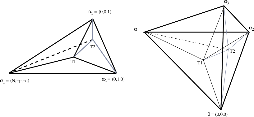
Figure 2: The fan of cones for the ${\mathbb{N}}$ lattice of ${\mathbb{C}}^{3}/{\mathbb{Z}}_{N(p,q)}$, with the vertices of the simplex $\Delta$, as well as tachyons $T_{1},T_{2}$ in the interior of the cone and the corresponding subdivisions thereof. (The figure on the left shows the simplex and its subdivision; the figure on the right shows the actual cones in the fan.)

Subcones of the cone $C(0;\alpha_{1},\alpha_{2},\alpha_{3})$ which have (real) dimension $p$ determine “toric” codimension-$p$ algebraic subspaces of ${\mathbb{C}}^{3}/{\mathbb{Z}}_{N(p,q)}$ with (complex) codimension $p$. Thus toric divisors (which are algebraically embedded codimension one subspaces) are determined by 1-dimensional cones, i.e. rays in $C(0;\alpha_{1},\alpha_{2},\alpha_{3})$.

Note that the cone $C(0;\alpha_{1},\alpha_{2},\alpha_{3})$ has volume $N$ in terms of the units defined by the lattice ${\mathbb{N}}$. The relationship between the group action and the lattice ${\mathbb{N}}$ in our case is visible in the basis in eqn. (17). In general, a cone with volume $k>1$ corresponds to an orbifold singularity by a discrete group $\Gamma$ whose order is $k$. (If cyclic, this is automatically a ${\mathbb{Z}}_{k}$ singularity.) To determine the group $\Gamma$, one needs a basis for the lattice ${\mathbb{N}}$ which is nicely adapted to the group action, in a manner analagous to eqn. (17). In fact, ${\mathbb{N}}$ is a lattice of rank 3 contained in the standard lattice ${\mathbb{Z}}^{3}$, and the group $\Gamma$ is the quotient ${\mathbb{Z}}^{3}/{\mathbb{N}}$, which is a finite group. The fact that a finitely generated abelian group is a direct sum of cyclic groups is a standard theorem in algebra (see, for example, [24]), and a specific algorithm to calculate the sum of cyclic groups – the “Smith normal form” – will be presented in section 4.

The simplex $\Delta$ is the intersection of the fan with an affine hyperplane passing through the three vertices $\alpha_{i}$. The equation describing the affine hyperplane containing the simplex $\Delta$ takes the form $\ell_{\Delta}(x,y,z)=1$, where

$$\ell_{\Delta}(x,y,z)=\biggl{(}{1+p+q\over N}\biggr{)}x+y+z.$$ (18)

We will refer to this affine hyperplane also as $\Delta$. The normal to the hyperplane $\Delta$ is the vector $v_{\bot}=(1+p+q,N,N)$, which satisfies $\alpha_{i}\cdot v_{\bot}=N>0$. The left side of figure 2 shows the affine hyperplane and the simplex $\Delta$ within it.

There is a remarkable correspondence between operators in the orbifold conformal field theory and subspaces in the ${\mathbb{N}}$ lattice. A given orbifold conformal field theory has relevant/marginal/irrelevant operators that correspond to specific lattice points in ${\mathbb{N}}$. In our normalization, the linear function $\ell_{\Delta}$ evaluated on a specific lattice point $j$ yields a value $\Delta_{j}=\ell_{\Delta}(x_{j},y_{j},z_{j})$ which is $equal$ to the R-charge $R_{j}$ of the corresponding operator. A given lattice point $P_{j}=(x_{j},y_{j},z_{j})$ can then be translated to an twisted sector operator as follows: realize that this vector can be expressed in the $\{\alpha_{1},\alpha_{2},\alpha_{3}\}$ basis as

$$(x_{j},y_{j},z_{j})=a\alpha_{1}+b\alpha_{2}+c\alpha_{3}.$$ (19)

This then corresponds to an operator $O_{j}$ with R-charge

$$R_{j}\equiv(a,b,c)=\biggl{(}{x_{j}\over N},\ y_{j}+x_{j}{p\over N},\ z_{j}+x_{j}{q\over N}\biggr{)}.$$ (20)

Conversely, an operator $O_{j}$ with R-charge $R_{j}=({j\over N},\{{jp\over N}\},\{{jq\over N}\})$ corresponds to a lattice point $P_{j}=(j,-[{jp\over N}],-[{jq\over N}])$. In general, there are lattice points lying “above” the affine hyperplane $\Delta$ that correspond to irrelevant deformations. These have $R_{j}=\Delta_{j}>1$.

Conformal field theories corresponding to supersymmetric ${\mathbb{C}}^{3}/{\mathbb{Z}}_{N}$ orbifolds always have marginal deformations that are represented by points $\beta_{k}$ that lie $on$ the affine hyperplane $\Delta$. Thus $R_{j}=\Delta_{j}=1$ for the $\beta_{k}$ and we will refer to the affine hyperplane $\Delta$ as the plane of marginal operators. The toric picture of blowing up a supersymmetric orbifold by a marginal operator then consists of adding to the cone an irreducible divisor (i.e. a ray) corresponding to the marginal operator $\beta_{k}$ and triangulating $\Delta$ into smaller sub-simplices that each have $\beta_{k}$ as a vertex. Such a subdivision of $\Delta$ by one or more of the $\beta_{k}$ gives a subdivision of the cone into subcones, corresponding to a blowup that gives a (partial) resolution of the orbifold singularity. Subdividing maximally using all the marginal operators (i.e. all the blowup modes) present resolves the orbifold completely so that the resulting space is smooth. See e.g. figure 5 of [20] for a picture of the supersymmetric ${\mathbb{C}}^{3}/{\mathbb{Z}}_{11}\ (1,3,-4)$ orbifold. In general, there are multiple distinct ways to subdivide using the $\beta_{k}$ in codimension three, which give resolved spaces of different topologies: these are related by flop transitions. Since the $\beta_{k}$ lie on $\Delta$, the maximal subdivision always yields $N$ minimal subcones each of volume one, making up the volume $N$ of the original cone.

In the nonsupersymmetric cases we study here, in addition to possible $\beta_{k}$ that lie $on$ $\Delta$ corresponding to marginal deformations, there are points $T_{k}$ in the interior of the cone (i.e. “below” the affine hyperplane $\Delta$) that correspond to relevant (tachyonic) deformations. These have $R_{j}=\Delta_{j}<1$.

As we have seen in the previous section, the chiral ring of twist field operators is generated by a subset comprising relevant, marginal and irrelevant operators. From the point of view of the toric representation we have described here, the relations $X_{a}\sim X_{g_{1}}^{m_{1}}X_{g_{2}}^{m_{2}}\ldots$ between various twist operators and the generators (see e.g. (14)) are precisely equivalent to the different possible ways to generate a given lattice vector by adding lattice vectors corresponding to generators.

The cone corresponding to a nonsupersymmetric singularity can be subdivided by the points $T_{k}$ as well as the $\beta_{k}$. Figure 2 shows tachyons $T_{1}$ and $T_{2}$ and their corresponding subdivisions. Such a tachyonic subdivision by a $T_{k}$ results in a partially-resolved space with total subcone-volume less than $N$, the volume of the original cone: in other words, the resulting space is less singular than the original orbifold. In general, if there are multiple tachyonic points $T_{k}$ in the interior, there are multiple distinct ways to subdivide which correspond to distinct resolutions of the original singularity, typically with distinct total volumes of the subcones. In other words, there is in general no canonical resolution. Some of these distinct resolutions are related by what are known as flip transitions. On the other hand, distinct subdivisions which give identical total volumes of their corresponding subcones are potentially related by flop transitions. In general the subcones obtained after all the subdivisions have been executed need not have volume $V_{subcone}=1$ each: the endpoint of maximal subdivisions corresponding to a generic collection of tachyons in ${\mathbb{C}}^{3}/{\mathbb{Z}}_{N(p,q)}$ includes subcones of volume $V_{subcone}>1$. Such a subcone corresponds to a $geometric$ terminal singularity, with no further lattice points on its affine hyperplane $\Delta_{subcone}$ or in the interior thereof: thus there are no further relevant or marginal chiral deformations of the corresponding conformal field theory by which it can be resolved via Kähler blowups. In the next section, we will elaborate more on these phenomena.

4 Geometric terminal singularities, flip transitions and all that

Unlike complex codimension one and two orbifold singularities, nonsupersymmetric (codimension three) ${\mathbb{C}}^{3}/{\mathbb{Z}}_{N(p,q)}$ orbifolds generically include “geometric” terminal singularities, containing no marginal or relevant Kähler blowup modes – a phenomenon well-known in algebraic geometry [25]. In physical terms, the corresponding worldsheet string conformal field theories do not contain any chiral relevant or marginal twisted sector operator by which the singularities can be resolved. A simple example is ${\mathbb{C}}^{3}/{\mathbb{Z}}_{2}\ (1,1,1)$: the twisted state from the only sector $j=1$ has R-charge $R_{j}={3\over 2}>1$, corresponding to an irrelevant operator in conformal field theory. More generally, it is easy to see that ${\mathbb{C}}^{3}/{\mathbb{Z}}_{N(p,-p)}$ is a geometric terminal singularity for $p,N$ coprime: the R-charge of the $j$-th twisted state is $R_{j}=1+{j\over N}>1$, so that the $(c_{X},c_{Y},c_{Z})$ (chiral) twist fields in each twisted sector correspond to irrelevant operators in the conformal field theory.

This result is further strengthened by the fact that toric ${\mathbb{C}}^{3}/{\mathbb{Z}}_{N}$ orbifold singularities have no complex structure deformations [26], unlike ${\mathbb{C}}^{2}/{\mathbb{Z}}_{N}$: resolutions must be by Kähler blowup modes.

On the other hand, sometimes the singularities can indeed be resolved. A simple example that is devoid of the intricacies to follow later is:

Figure 3: ${\mathbb{C}}^{3}/{\mathbb{Z}}_{N}\ (1,1,1)$ : The three points defining the affine hyperplane $\Delta$ are shown, along with the sole tachyon $T_{1}$ and its corresponding subdivision.

Example ${\mathbb{C}}^{3}/{\mathbb{Z}}_{N}\ (1,1,1)$:  Figure 3 shows the vertices $(N,-1,-1),(0,1,0),(0,0,1)$ of the cone in the toric diagram. For $N=3$, this can be recast as the familiar supersymmetric ${\mathbb{Z}}_{3}$ orbifold, while for $N>3$ there is a single tachyonic operator $T_{1}=(1,0,0)$ with R-charge $R_{j}={3\over N}$ that generates the chiral ring (shown in the figure). The operators $T_{j}=(j,0,0)$ with R-charges $R_{j}={j\over N}$ are tachyonic for $j<N$ and are generated by $T_{1}$: the $T_{j}$ are collinear with the generator $T_{1}$ and the origin. As can be seen from figure 3, the three subcones arising from the subdivision by $T_{1}$ have volumes $V(0;\alpha_{1},\alpha_{2},T_{1})=V(0;\alpha_{2},\alpha_{3},T_{1})=V(0;\alpha_{3},\alpha_{1},T_{1})=1\$ for any $N$, so that condensation of the most relevant tachyon $T_{1}$ here leads to a resolution of the orbifold to flat space.

Minimal resolutions, terminal singularities, and flips
The traditional mathematical approach to studying resolutions of singularities (orbifold or otherwise) proceeds in two steps. First, thanks to a famous theorem of Hironaka [8], it is known that there is a sequence of (Kähler) blowups which yields a smooth space. However, this resolution is far from unique, because it is possible to perform arbitrary additional blowups along smooth subvarieties of the smooth space, yielding other resolutions. The question thus arises: can we find some kind of “minimal” resolution of a singularity?

In complex dimension one, further blowups do not change the space and the question does not arise. In complex dimension two, the existence of a unique minimal resolution of singularities follows from the results of the classical Italian school of algebraic geometry (from the first half of the twentieth century). The analogous question in complex dimension three was the subject of intense efforts by mathematicians in the 1980’s.

When studying nonlinear sigma models, the possibility of arbitrary blowups along smooth subvarieties is not an issue for the physical theory, because such blowups correspond to irrelevant operators in the sigma model [9]. In fact, the classification of sigma model operators into relevant, marginal, and irrelevant exactly parallels the criterion introduced by Mori [28] to attack the minimal resolution question: Mori studied the sign of the intersection numbers $K_{X}\cdot C$, where $K_{X}$ is the algebraic divisor class measuring the zeros and poles of a holomorphic $n$-form, and $C$ is an arbitrary algebraic curve on $X$. When $K_{X}\cdot C<0$, the sigma model operator which creates $C$ via a blowup is irrelevant; when $K_{X}\cdot C=0$ the operator is marginal; and when $K_{X}\cdot C>0$ the operator is relevant.

Mori showed that starting from a smooth complex threefold, if there are any $C$’s with $K_{X}\cdot C<0$, then there is always a blowdown map which shrinks some of those $C$’s to zero size. (This is precisely what we would expect from analyzing the sigma model, since such $C$’s correspond to irrelevant operators.) In complex dimension two, the blowdown yields a smooth surface, but in complex dimension three, the blowdown can introduce singularities, the so-called terminal singularities. By definition (see, e.g., [25]), these are singularities for which some tensor power $(\Omega^{n})^{\otimes r}$ of the sheaf of holomorphic $n$-forms has local sections, with the property that for every blowup, the pullback of any local section of $(\Omega^{n})^{\otimes r}$ vanishes along each divisor created by the blowup. In the case of orbifold singularities, this rather technical condition can be replaced by a simpler condition (which is equivalent to checking for relevant or marginal tachyons), and the terminal orbifold singularities in complex dimension three can be completely classified [29].

Later study revealed that a minimal resolution could not be reached by simply following a sequence of blowdowns from the starting resolution: in addition, one needs to consider “flips,” in which (locally) a single curve $C$ on $X$ shrinks to zero size, but then a different blowup is done which causes a new curve $C^{+}$ to grow, creating the space $X^{+}$. We have $K_{X}\cdot C<0$ but $K_{X^{+}}\cdot C^{+}>0$. (Both spaces $X$ and $X^{+}$ have terminal singularities—there are no flips which just involve smooth spaces.) Work by Reid, Kawamata and others culminated in the final result by Mori [30] which showed that minimal resolutions exist and can be obtained from arbitrary resolutions by a sequence of blowdowns and flips.

In fact, the theorem had earlier been proven in the case of toric blowups, blowdowns, and flips by Danilov [31]. The combinatorics of this process on toric varieties is the tool we are using here.

Relevance of tachyons, volume minimization and flips
In general, for the orbifolds being studied in this paper, there are multiple tachyons not collinear with the origin in the interior of the cone with distinct R-charges i.e. order of relevance, thus giving rise to distinct subdivisions and potential flip (or flop) transitions between the distinct subdivisions. As we have mentioned before, the most relevant tachyon (smallest R-charge) is the dominant perturbation of the worldsheet theory, and correspondingly the dominant unstable direction from the point of view of the target spacetime (most negative $M^{2}$). Thus the most relevant tachyon is most likely to condense, followed by the next most relevant tachyon and so on. In the ${\mathbb{C}}^{2}/{\mathbb{Z}}_{N(p)}$ cases, the Hirzebruch-Jung minimal resolution theory ensures that the final endpoint of this sequence of most relevant tachyons is a set of decoupled flat space regions (see Appendix B). ${\mathbb{C}}^{3}/{\mathbb{Z}}_{N(p,q)}$ however has richer structure: the generic sequence of tachyonic perturbations leads to geometric terminal singularities as we have mentioned above. Furthermore, tachyons with different degrees of “tachyonity”, i.e. relevance of R-charge, give rise with different degrees of likelihood to resolutions which generically have distinct topologies. There is an interesting calculation that shows the relation between the relevance (R-charges) of distinct tachyons and the ${\mathbb{N}}$ lattice volumes of the subcones resulting from the subdivisions corresponding to those tachyons, i.e. the degree of singularity of the residual geometry. Let us begin with the cone $C(0;\alpha_{1},\alpha_{2},\alpha_{3})$ corresponding to the unresolved ${\mathbb{C}}^{3}/{\mathbb{Z}}_{N(p,q)}$ singularity. Now add a lattice point $T_{j}=(j,-[{jp\over N}],-[{jq\over N}])$ corresponding to a tachyon $T_{j}$. Then the total volume of the three residual subcones after subdivision with the tachyon $T_{j}$ is easily calculated: let $V(e_{0};e_{1},e_{2},e_{3})$ denote the volume of a cone subtended by the vectors $e_{1},e_{2},e_{3}$ with the vector $e_{0}$ being the apex. Then (see e.g. figure 2) we have

$$V_{subcones}(T_{j}) = V(0;\alpha_{1},\alpha_{2},\alpha_{3})-V(T_{j};\alpha_{1},\alpha_{2},\alpha_{3})$$ (21)

$$= \alpha_{1}\cdot(\alpha_{2}\times\alpha_{3})-\biggl{[}(\alpha_{1}-T_{j})\cdot(\alpha_{2}-T_{j})\times(\alpha_{3}-T_{j})\biggr{]}=N-N(1-R_{j})$$

$$= NR_{j}<N.$$

Now if we consider two tachyons $T_{1}$ and $T_{2}$ (as in figure 2), such that $T_{1}$ is more relevant than $T_{2}$, i.e.

$$R_{1}<R_{2},\qquad\qquad R_{i}={j_{i}\over N}+\biggl{\{}{j_{i}p\over N}\biggr{\}}+\biggl{\{}{j_{i}q\over N}\biggr{\}}.$$ (22)

This implies

$$V_{subcones}(T_{1})<V_{subcones}(T_{2}).$$ (23)

This shows that given a singularity, condensation of a more relevant tachyon locally leads to a less singular partial resolution. For instance, imagine that the less relevant tachyon $T_{2}$ begins to condense (figure 1): if left unperturbed, the singularity will decay and settle down to the resolution with three decoupled sub-singularities with total volume $V_{subcones}(T_{2})$ of the three corresponding subcones. However, in the process of decay, if a small fluctuation causes condensation of the more relevant $T_{1}$, this will dominate over the earlier blowup causing a $flip$ transition that dynamically forces the singularity to settle down to the less singular resolution with volume $V_{subcones}(T_{1})<V_{subcones}(T_{2})$. From the point of view of the toric diagram, condensing the tachyon $T_{j}$ by blowing up the corresponding divisor is associated with adding the corresponding lattice point (and the ray thereof) and subdividing thereby. Likewise blowing down a divisor corresponds to removing its associated ray and the subdivision thereof. In this language, a flip transition can be thought of in a manner similar to a flop: as a blowdown combined with a blowup, except that in this case there is an associated potential hill owing to the fact that relevant operators are at work here (we remind the reader that a flop consists of truly marginal deformations lying on the moduli space of supersymmetric string vacua). For instance in figure 1, endpoint 1 is less singular than endpoint 2: thus there is a potential hill for the flip transition $2\rightarrow 1$.

For either partial resolution, the residual subcones generically have further tachyons themselves, i.e. the resulting system is itself unstable to tachyon condensation. Thus iterating the above argument sequentially suggests that sequential condensation of the most relevant tachyons (instead of condensation of generic tachyons) is what leads to a decoupled set of residual singularities that is as flat as possible, i.e. with minimal total volume $V_{subcones}$ for the entire set of subcones. However the local argument for the inequality above does not shed light on the global question of whether sequentially condensing the most relevant tachyon indeed leads to the least singular endpoint, i.e. whether the resulting stable singularity (with no further tachyons) has minimum total ${\mathbb{N}}$ lattice volume $V_{subcones}$.

The Smith normal form
Let us now ask what the structure of the residual singularities is. For instance (see figure 2) we obtain the three decoupled subcones $C(0;T_{1},\alpha_{1},\alpha_{2}),C(0;T_{1},\alpha_{2},\alpha_{3}),C(0;T_{1},\alpha_{3},\alpha_{1})$ as the endpoint of the condensation of the first tachyon, say, $T_{1}$. Each of these residual subcones represents a new orbifold conformal field theory (decoupled from the other theories corresponding to the other subcones) which itself generically contains further tachyons. In general, such a residual subcone, defined by three lattice points, is an orbifold singularity whose associated group is determined by the lattice points. Abstractly, it is easy to say what the group is: the three lattice points generate a subgroup ${\mathbb{M}}$ of the standard lattice ${\mathbb{Z}}^{3}$, and the quotient group ${\mathbb{Z}}^{3}/{\mathbb{M}}$ coincides with the orbifold group $\Gamma$. By a standard theorem in abstract algebra [24], such a quotient group can always be written as a direct sum of cyclic groups.

Concretely, the group $\Gamma$ associated with such a singularity can be calculated efficiently by an algorithm which puts an integer matrix into the so-called Smith normal form. The integer matrix in question describes the inclusion of ${\mathbb{M}}$ into ${\mathbb{Z}}^{3}$ (via a choice of generators), and the Smith normal form algorithm produces a new choice of generators which makes the structure as a direct sum of cyclic groups manifest (as well as indicating the group action for each of the summands). This is best illustrated by an example. For a given subcone, say $C(0;T_{1},\alpha_{2},\alpha_{3})$, consider the matrix formed by juxtaposing the column vectors $T_{1},\alpha_{2},\alpha_{3}$ representing the subcone vertices and performing the following set of elementary row and column operations on it to eventually obtain a diagonal matrix

$$\left(\begin{array}[]{ccc}j_{1}&0&0\\ -[{j_{1}p\over N}]&1&0\\ -[{j_{1}q\over N}]&0&1\\ \end{array}\right)\ \rightarrow\ \left(\begin{array}[]{ccc}j_{1}&0&0\\ -[{j_{1}p\over N}]&1&0\\ 0&0&1\\ \end{array}\right)\ \rightarrow\ \left(\begin{array}[]{ccc}j_{1}&0&0\\ 0&1&0\\ 0&0&1\\ \end{array}\right).$$ (33)

We have performed the operations $\ T_{1}+[{j_{1}p\over N}]\alpha_{2}\$ and $\ T_{1}+[{j_{1}p\over N}]\alpha_{2}+[{j_{1}q\over N}]\alpha_{3}\$ on the first column, in the first and second step here. This then corresponds to the singularity ${\mathbb{Z}}_{j_{1}}$, with action $(1,[{j_{1}p\over N}],[{j_{1}q\over N}])$ on the three coordinates represented by the vertices $T_{1},\alpha_{2},\alpha_{3}$.

More generally, begin with the matrix formed by juxtaposing the column vectors $v_{1},v_{2},v_{3}\in{\mathbb{Z}}^{3}$ representing the vertices of a given subcone $C(0;v_{1},v_{2},v_{3})$ and perform elementary row and column operations to obtain a diagonal matrix $\ {\rm diag}[d_{1},d_{2},d_{3}]$, with $\ d_{3}|d_{2}|d_{1}$, as the Smith normal form of the original matrix: this corresponds to a ${\mathbb{Z}}_{d_{1}}\times{\mathbb{Z}}_{d_{2}}\times{\mathbb{Z}}_{d_{3}}$ singularity. The Smith normal form algorithm essentially executes $GL(3,{\mathbb{Z}})$ transformations on the lattice vectors as well as on the lattice basis itself: column operations change the lattice vectors while row operations are simply a change of basis of the lattice which thus do not affect the relations between the lattice vectors (and therefore the structure of the orbifold action). Note that generically both column and row operations are required to obtain the Smith normal form, putting the lattice vectors describing the orbifold into canonical form. As another example, consider the following matrix which appears for the subcone $C(0;T_{2},\alpha_{1},\alpha_{2})$ in ${\mathbb{C}}^{3}/{\mathbb{Z}}_{11}\ (1,2,7)$

$$\left(\begin{array}[]{ccc}11&0&2\\ -2&1&0\\ -7&0&-1\\ \end{array}\right)\ \rightarrow\ \left(\begin{array}[]{ccc}11&0&2\\ 0&1&0\\ -7&0&-1\\ \end{array}\right)\ \rightarrow\ \left(\begin{array}[]{ccc}-3&0&2\\ 0&1&0\\ 0&0&-1\\ \end{array}\right)\ \rightarrow\ \left(\begin{array}[]{ccc}-3&0&0\\ 0&1&0\\ 0&0&-1\\ \end{array}\right).$$ (46)

We have performed the column operations $\ \alpha_{1}+2\alpha_{2}\$ and $\ \alpha_{1}+2\alpha_{2}-7T_{2}\$ on the first column, in the first and second step here, followed by a row operation $r_{1}+2r_{3}$ in the third step. This thus corresponds to a ${\mathbb{Z}}_{3}\ (-7,1,2)$ singularity (the orbifold actions are on $T_{2},\alpha_{1},\alpha_{2}$ respectively), which is the same as ${\mathbb{Z}}_{3}\ (-1,1,2)$. We will find more intricate use for this algorithm in what follows.

There is an alternate equivalent way of realizing the orbifold action, which is to find a linear combination of the vertices in question that is itself a vector in the lattice generated by the vertices. As an example, it is clear from our first example above that the vector $\ {1\over j_{1}}(T_{1}+[{j_{1}p\over N}]\alpha_{2}+[{j_{1}q\over N}]\alpha_{3})=(1,0,0)\$ is clearly a lattice point itself: from this we read off the orbifold action to be ${\mathbb{Z}}_{j_{1}}\ (1,[{j_{1}p\over N}],[{j_{1}q\over N}])$ as above. In the second example above, we have $\ -{1\over 3}(-7T_{2}+\alpha_{1}+2\alpha_{2})=(1,0,0)\$ as a lattice vector, giving ${\mathbb{Z}}_{3}\ (-7,1,2)\equiv{\mathbb{Z}}_{3}\ (-1,1,2)$ as above.

It is important to note that the vector that arises as the linear combination in the Smith normal form is only defined up to linear combinations of integral multiples of the original lattice vectors.

Renormalization of subsequent tachyons within subcones
As mentioned previously, a tachyonic chiral operator that condenses breaks the full ${\cal N}=(2,2)$ worldsheet supersymmetry down to the subgroup preserved by the ring it belongs to (say $(c_{X},c_{Y},c_{Z})$). Furthermore, the residual theories arising at the endpoint of condensation of a given tachyon have different R-symmetries from the original conformal field theory. Thus the R-charges of the subsequent tachyons remaining in the residual geometries get “renormalized” after a given tachyon has condensed, the specific renormalization of a particular subsequent tachyon depending on which of the three decoupled subcones it lies within. A subsequent tachyon in a residual subcone is a chiral operator with respect to the R-symmetries preserved by that subcone. In figure 2 for instance, the subsequent tachyon $T_{2}$ lies in the subcone $C(0;\alpha_{2},\alpha_{3},T_{1})$. It is then easy to see that the R-charge of $T_{2}$ is in general different, since its geometry relative to the affine hyperplane $\Delta_{subcone}$ (the plane passing through the subcone vertices $T_{1},\alpha_{2},\alpha_{3}$) is different from before. Since $\Delta_{subcone}$ dips inwards, in other words away from the original $\Delta_{cone}$, a subsequent tachyon is always closer to $\Delta_{subcone}$ (corresponding to the subcone it lies within). Thus the renormalized R-charges of subsequent tachyons are always greater than their prior values.

This renormalization of the R-charge can be calculated by studying the geometry of the subsequent tachyon in question relative to the subcone it lies within (the expressions appearing below can be checked for agreement with $R_{k}^{\prime}=a+b+c$ calculated for $T_{k}$ lying in a subcone in the next section on Type II theories). The equation describing an affine hyperplane $\Delta_{subcone}$ passing through three lattice points $v_{1}=(x_{1},y_{1},z_{1}),v_{2}=(x_{2},y_{2},z_{2}),v_{3}=(x_{3},y_{3},z_{3})$ can be written as

$$\ell_{\Delta_{subcone}}(x,y,z)\equiv{D(x,y,z)\over D(x_{1},y_{1},z_{1})}=1,\quad D(x,y,z)=\det\left(\begin{array}[]{ccc}x&y&z\\ x_{2}-x_{1}&y_{2}-y_{1}&z_{2}-z_{1}\\ x_{3}-x_{1}&y_{3}-y_{1}&z_{3}-z_{1}\\ \end{array}\right).$$ (50)

This has been normalized so that a lattice point lying on $\Delta_{subcone}$ corresponds to a marginal operator with R-charge $R_{j}=\ell_{\Delta_{subcone}}(x_{j},y_{j},z_{j})={D(x_{j},y_{j},z_{j})\over D(x_{1},y_{1},z_{1})}=1$. To illustrate this expression, consider the subsequent tachyon $T_{2}$ in the residual subcone $C(0;T_{1},\alpha_{2},\alpha_{3})$ in figure 2. Then the renormalized R-charge of $T_{2}$ after $T_{1}$ has condensed can be read off from the equation describing $\Delta_{subcone}$ through $T_{1},\alpha_{2},\alpha_{3}$ (simplifying the above expression using (13) for the R-charge) as

$$R_{2}^{\prime}=\ell_{\Delta^{23T}}(T_{2})\equiv{D^{23T}(T_{2})\over D^{23T}(T_{1})}=R_{2}+{j_{2}\over j_{1}}\biggl{(}1-R_{1}\biggr{)}=R_{2}\ \biggl{[}1+{j_{2}\over j_{1}}\ {(1-R_{1})\over R_{2}}\biggr{]}.$$ (51)

Similarly, the corresponding expressions for the renormalized R-charge if the subsequent tachyon $T_{2}$ lies within the residual subcones $C(0;T_{1},\alpha_{1},\alpha_{2})$ or $C(0;T_{1},\alpha_{3},\alpha_{1})$ in figure 2 are

$$R_{2}^{\prime}=\ell_{\Delta^{12T}}(T_{2})\equiv{D^{12T}(T_{2})\over D^{12T}(T_{1})}=R_{2}\ \biggl{[}1+{\{{j_{2}q\over N}\}\over\{{j_{1}q\over N}\}}\ {(1-R_{1})\over R_{2}}\biggr{]},\qquad\qquad T_{2}\in(0;T_{1},\alpha_{1},\alpha_{2}),\ \$$

$$R_{2}^{\prime}=\ell_{\Delta^{31T}}(T_{2})\equiv{D^{31T}(T_{2})\over D^{31T}(T_{1})}=R_{2}\ \biggl{[}1+{\{{j_{2}p\over N}\}\over\{{j_{1}p\over N}\}}\ {(1-R_{1})\over R_{2}}\biggr{]},\qquad\qquad T_{2}\in(0;T_{1},\alpha_{3},\alpha_{1}).$$

It is easy to see that since we are considering tachyons, we have $R_{1}<1$ so that $R_{2}^{\prime}>R_{2}$ always. In the examples below, we will illustrate this fact with several subsequent tachyons that become marginal or near-marginal or irrelevant.

We now present a Type 0 example describing the tachyons therein and the toric blowups thereof. It is useful to keep in mind the supersymmetric ${\mathbb{C}}^{3}/{\mathbb{Z}}_{11}\ (1,3,-4)$ orbifold that is studied in some detail in [20].

Example ${\mathbb{C}}^{3}/{\mathbb{Z}}_{13}\ (1,2,5)$:  See figure 4. The most relevant tachyon in the Type 0 theory in this example lies in the $(c_{X},c_{Y},c_{Z})$ ring and is $T_{1}=({1\over 13},{2\over 13},{5\over 13})$ with R-charge $R_{1}={8\over 13}$. This ring also has the tachyons $T_{3}=({3\over 13},{6\over 13},{2\over 13})$ and $T_{8}=({8\over 13},{3\over 13},{1\over 13})$ with R-charges  $R_{3}={11\over 13}$ and $R_{8}={12\over 13}\$ respectively. In the toric fan (with vertices $\alpha_{1}=(13,-2,-5),\ \alpha_{2}=(0,1,0),\ \alpha_{3}=(0,0,1)$), these tachyons correspond to the lattice vectors $T_{1}=(1,0,0),\ T_{3}=(3,0,-1),\ T_{8}=(8,-1,-3)$. As can be seen from the volumes below (or otherwise), $T_{1}$ and $T_{3}$ are coplanar with $\alpha_{3}$ while $T_{3}$ and $T_{8}$ are coplanar with $\alpha_{1}$. For convenience, we note down here the volumes of some subcones that arise in the subdivisions we will describe below

$${}V(\alpha_{1},T_{3},T_{8})=V(\alpha_{3},T_{1},T_{3})=0,\ \ \ V(\alpha_{2},\alpha_{3},T_{1})=V(T_{3},T_{1},T_{8})=V(\alpha_{1},T_{1},T_{8})=1,\ \$$

$${}V(\alpha_{1},\alpha_{2},T_{3})=V(\alpha_{1},\alpha_{3},T_{1})=2,\ \ V(\alpha_{1},\alpha_{3},T_{8})=3,\ \ V(\alpha_{1},\alpha_{2},T_{1})=5,\ \$$

$${}V(\alpha_{3},T_{1},T_{8})=V(\alpha_{1},\alpha_{2},T_{8})=V(\alpha_{2},T_{3},T_{8})=V(\alpha_{2},T_{1},T_{3})=1\ \$$ (53)

Figure 4: ${\mathbb{C}}^{3}/{\mathbb{Z}}_{13}\ (1,2,5)$ : The three points defining the affine hyperplane $\Delta$ are shown, along with the three tachyons $T_{1},T_{3},T_{8}$ and two distinct sequences of subdivisions. The solid lines correspond to the sequence of most relevant tachyons.

Let us first consider the subdivisions shown by the solid lines which correspond to sequentially blowing up the most relevant tachyon, i.e. the sequence $T_{1},\ T_{3},\ T_{8}$: this gives the total volume of the subcones to be $6(1)+2$, which is smaller and thus will dynamically give rise to a flip transition. Let us consider this sequence in more detail: the first subdivision by $T_{1}$ gives the three subcones $C(0;\alpha_{3},T_{1},\alpha_{2}),\ C(0;\alpha_{1},T_{1},\alpha_{3}),\ C(0;\alpha_{1},\alpha_{2},T_{1})$, which by the Smith normal form are respectively flat space, ${\mathbb{Z}}_{2}$ and ${\mathbb{Z}}_{5}\ (1,2,-3)$ singularities. Alternatively it is straightforward to realize the combinations  ${1\over 5}(-\alpha_{1}-2\alpha_{2}+13T_{1})=(0,1,0)$ and  ${1\over 2}(-\alpha_{1}-5\alpha_{3}+13T_{1})=(0,1,0)$ as vectors in the lattice: these imply that the subcones $C(0;\alpha_{1},\alpha_{2},T_{1})$ and $C(0;\alpha_{1},T_{1},\alpha_{3})$ are respectively ${\mathbb{Z}}_{5}\ (1,2,-13)\equiv{\mathbb{Z}}_{5}\ (1,2,-3)$ and ${\mathbb{Z}}_{2}\ (1,5,-13)\equiv{\mathbb{Z}}_{2}\ (1,1,-1)$ singularities (shifting by multiples of the corresponding lattice vectors). Thus the three decoupled residual geometries after this subdivision by the most relevant tachyon $T_{1}$ include a terminal singularity along with a supersymmetric orbifold with only marginal blowup modes (i.e. no relevant blowup modes). Using (51) and (4), we can calculate the renormalized R-charges of the subsequent twisted states as

$$R_{3}^{\prime}=\ell_{\Delta^{12T}}(T_{3})={D^{12T}(T_{3})\over D^{12T}(T_{1})}=1,\qquad R_{8}^{\prime}=\ell_{\Delta^{12T}}(T_{8})={D^{12T}(T_{8})\over D^{12T}(T_{1})}=1.$$ (54)

The R-charges can also equivalently be calculated directly by realizing that the corresponding plane is described by $\ x+y+2z=1$ and using this to see that the erstwhile tachyons now lie $on$ this plane.

On the other hand, choosing a different sequence of tachyons by which to fully subdivide the cone gives rise to different fans of subcones. For instance, the dotted line in figure 4 shows a subdivision corresponding to the sequence $T_{3},\ T_{8},\ T_{1}$. From the combinations ${1\over 3}(\alpha_{3}+T_{3})=(1,0,0)$,  ${1\over 6}(13T_{3}-2\alpha_{3}-3\alpha_{1})=(0,1,0)$ and  ${1\over 2}(-3\alpha_{1}-6\alpha_{2}+13T_{3})=(0,0,1)$ of the lattice vectors, we see that the subdivision by $T_{3}$ gives the subcones $C(0;\alpha_{2},\alpha_{3},T_{3}),\ C(0;T_{3},\alpha_{3},\alpha_{1}),\ C(0;\alpha_{1},\alpha_{2},T_{3})$, to be ${\mathbb{Z}}_{3}\ (0,1,1),\ {\mathbb{Z}}_{6}\ (13,-2,-3)\equiv{\mathbb{Z}}_{6}\ (1,-2,-3)$ and ${\mathbb{Z}}_{2}\ (-3,-6,13)\equiv{\mathbb{Z}}_{2}\ (1,0,1)$ singularities respectively. Further it is easy to see that $T_{1}={1\over 3}(T_{3}+\alpha_{3})$ and $T_{8}={1\over 2}(T_{3}+\alpha_{1})$ : thus $T_{8}$ becomes marginal after the blowup by $T_{3}$ while $T_{1}$ acquires the R-charge $R_{1}^{\prime}={2\over 3}>{8\over 13}$. One can now subdivide by the remaining relevant tachyons to obtain the total volume of the subcones to be $6(1)+3$ (from the list of volumes above): this is greater than the corresponding total volume in the most-relevant-tachyon subdivision, as we saw in general earlier.

5 Type II theories and all-ring terminality

As in the Type 0 theory (see Sec. 2), there are eight rings of operators (anti-)chiral under each of the three copies of the ${\cal N}{=}2$ superconformal algebra, in four conjugate pairs. The chiral GSO projection for Type II ${\mathbb{C}}^{d}/{\mathbb{Z}}_{N}$ theories preserves spacetime fermions and eliminates the bulk tachyon of the untwisted sector: further it acts nontrivially on these twist fields representing tachyons localized to the singular orbifold subspace, projecting out some of them. We will now describe the structure of the various rings in Type II theories in more detail. Unlike the supersymmetric ${\mathbb{C}}^{3}/{\mathbb{Z}}_{N(p,-p-1)}$ orbifolds where all the $R_{j}=1$ twisted states in the $(c_{X},c_{Y},c_{Z})$ ring, which comprise all the blowup modes of the singularity, are preserved and operators in the other rings are projected out, the chiral GSO projection for nonsupersymmetric orbifolds retains some localized tachyons in each ring, as we describe in greater detail below.

We recall (Appendix A) that for an orbifold ${\mathbb{C}}^{3}/{\mathbb{Z}}_{N}\ (k_{1},k_{2},k_{3})$ to allow a Type II chiral GSO projection admitting spacetime fermions, we must have $\sum_{i}k_{i}=even$. Localized closed string tachyons arise in those twisted sectors for which the action on the twist field operators is given by

$$X_{j}^{r}\rightarrow X_{j}^{r}\ (-1)^{E_{j}^{r}},$$ (55)

where the GSO exponent $E_{j}^{r}$ depends nontrivially on the twist sector $j$ as well as the specific (anti-)chiral ring $r$ that the twist field belongs to. From Appendix A.2 (see e.g. eqns. (189) (190)), the GSO exponents in Type II theories for twist field operators in the various rings of a ${\mathbb{C}}^{3}/{\mathbb{Z}}_{N}\ (k_{1},k_{2},k_{3})$ orbifold are

$$E_{j} = \sum_{i}\biggl{[}{jk_{i}\over N}\biggr{]},\qquad\qquad\qquad j=1,\ldots,N-1$$ (56)

$$= {\rm odd},\qquad\qquad X_{j}\ \in\ (c_{X},c_{Y},c_{Z}),(c_{X},a_{Y},a_{Z}),(a_{X},c_{Y},a_{Z}),(a_{X},a_{Y},c_{Z})$$

$$= {\rm even},\qquad\qquad X_{j}\ \in\ (c_{X},c_{Y},a_{Z}),(c_{X},a_{Y},c_{Z}),(a_{X},c_{Y},c_{Z}),(a_{X},a_{Y},a_{Z})$$

For example, a $(c_{X},c_{Y},c_{Z})$-ring twist field operator (in the $(-1,-1)$ picture)

$$X_{j}=\prod_{i=1}^{3}\ X^{i}_{\{jk_{i}/N\}}=\prod_{i=1}^{3}\ \sigma_{\{jk_{i}/N\}}\ e^{i\{jk_{i}/N\}(H_{i}-{\bar{H}}_{i})},$$ (57)

has its conjugate field

$$X_{j}^{*}=\prod_{i=1}^{3}\ (X^{i}_{\{jk_{i}/N\}})^{*}=\prod_{i=1}^{3}\ (X^{i}_{\{-(N-j)k_{i}/N\}})^{*}=\prod_{i=1}^{3}\ (X^{i}_{1-\{(N-j)k_{i}/N\}})^{*},$$ (58)

which clearly lies in the $(N-j)$-th twist sector in the conjugate ring $(a_{X},a_{Y},a_{Z})$. Now it is straightforward to see that if $X_{j}$ is preserved, so is its conjugate field in the conjugate ring:

$$E_{j} = \sum_{i}\biggl{[}{jk_{i}\over N}\biggr{]}={\rm odd}\Rightarrow$$

$$E_{N-j} = \sum_{i}\biggl{[}{(N-j)k_{i}\over N}\biggr{]}=\sum_{i}k_{i}+\sum_{i}\biggl{[}{-jk_{i}\over N}\biggr{]}=-E_{j}-3={\rm even}.$$ (59)

Similarly for the other rings and their conjugates.

As we have briefly mentioned in Sec. 2, there is a convenient notation that can be used to study and label twist operators in the various rings. To illustrate this, note that twist operators in the $(c_{X},c_{Y},a_{Z})$-ring can be rewritten as

$$X_{j}^{cca}=X^{1}_{\{jk_{1}/N\}}\ X^{2}_{\{jk_{2}/N\}}\ (X^{3}_{1-\{jk_{3}/N\}})^{*}=X^{1}_{\{jk_{1}/N\}}\ X^{2}_{\{jk_{2}/N\}}\ (X^{3}_{\{-jk_{3}/N\}})^{*},$$ (60)

which resemble twist operators in the $(c_{X},c_{Y},c_{Z})$ ring of the orbifold ${\mathbb{C}}^{3}/{\mathbb{Z}}_{N}\ (k_{1},k_{2},-k_{3})$ with $X^{3}\rightarrow(X^{3})^{*}$ : indeed the R-charges of the operators are identical while the condition on their GSO exponents

$$E_{j}=\sum_{i}\biggl{[}{jk_{i}\over N}\biggr{]}=even$$ (61)

can be re-expressed as

$$E_{j}^{cca} = \biggl{[}{jk_{1}\over N}\biggr{]}+\biggl{[}{jk_{2}\over N}\biggr{]}+\biggl{[}-{jk_{3}\over N}\biggr{]}$$ (62)

$$= E_{j}+1+{\rm even}={\rm odd},$$

so that as expected for a $(c_{X},c_{Y},c_{Z})$ ring operator, the corresponding GSO exponent $E_{j}^{cca}$ is odd. As another example, the $(a_{X},a_{Y},c_{Z})$ ring of ${\mathbb{C}}^{3}/{\mathbb{Z}}_{N}\ (k_{1},k_{2},k_{3})$ can be expressed as the $(c_{X},c_{Y},c_{Z})$ ring of the orbifold ${\mathbb{C}}^{3}/{\mathbb{Z}}_{N}\ (-k_{1},-k_{2},k_{3})$ with $X^{1}\rightarrow(X^{1})^{*},X^{2}\rightarrow(X^{2})^{*}$ . Generalizing, we see that operators in non-$(c_{X},c_{Y},c_{Z})$ rings of the ${\mathbb{C}}^{3}/{\mathbb{Z}}_{N}\ (k_{1},k_{2},k_{3})$ orbifold can be expressed as $(c_{X},c_{Y},c_{Z})$ ring operators of a corresponding orbifold with related weights. This interrelation between the structure of the various rings can be exploited to rewrite the GSO exponents for preserved twist operators in the various rings more conveniently, so that they are uniformly $odd$ as expected for the re-expressed $(c_{X},c_{Y},c_{Z})$ ring operators. We will find this rewriting of the GSO exponents particularly convenient to use when we discuss all-ring terminality (see e.g. eqn. (5)).

The GSO projection for subcones and residual tachyons within
We now come to the question of studying the geometry of subcones in greater detail, in particular in the light of the chiral GSO projection for Type II theories. Consider condensing a GSO-preserved twisted state $T_{j}=(j,-[{jp\over N}],-[{jq\over N}])\equiv({j\over N},\{{jp\over N}\},\{{jq\over N}\})$ in a Type II ${\mathbb{C}}^{3}/{\mathbb{Z}}_{N(p,q)}$ orbifold. Then the chiral GSO projection requires that $p+q=odd$ and $[{jp\over N}]+[{jq\over N}]=odd$. This gives three subcones $C(0;T_{j},\alpha_{2},\alpha_{3}),C(0;T_{j},\alpha_{1},\alpha_{2}),C(0;T_{j},\alpha_{3},\alpha_{1})$, which are orbifolds of the general form ${\mathbb{C}}^{3}/{\mathbb{Z}}_{n}\ (r^{\prime},p^{\prime},q^{\prime})$. In general these are not isolated. As we have seen from (33), $C(0;T_{j},\alpha_{2},\alpha_{3})$ is equivalent to the orbifold ${\mathbb{C}}^{3}/{\mathbb{Z}}_{j}\ (1,[{jp\over N}],[{jq\over N}])$, the orbifold action being on the coordinates represented by $T_{j},\alpha_{2},\alpha_{3}$ respectively. This clearly admits a Type II GSO projection since $r^{\prime}+p^{\prime}+q^{\prime}=1+[{jp\over N}]+[{jq\over N}]=even$. The other subcones are somewhat harder to nail down in general but in large classes of cases it is possible to glean insight using the toric data.

Consider the subcone $C(0;T_{j},\alpha_{3},\alpha_{1})$: using the Smith normal form or otherwise, we see that the vector

$$(1,0,0) = {1\over N\{{jp\over N}\}}\biggl{(}p(T_{j}+\biggl{[}{jq\over N}\biggr{]}\alpha_{3})-\biggl{[}{jp\over N}\biggr{]}(\alpha_{1}+q\alpha_{3})\biggr{)}$$ (63)

$$= {1\over N\{{jp\over N}\}}\biggl{(}pT_{j}-\biggl{[}{jp\over N}\biggr{]}\alpha_{1}+(p\biggl{[}{jq\over N}\biggr{]}-q\biggl{[}{jp\over N}\biggr{]})\alpha_{3})\biggr{)}$$

is in the original lattice, showing that the subcone $C(0;T_{j},\alpha_{3},\alpha_{1})$ is equivalent to the orbifold

$${\mathbb{C}}^{3}/{\mathbb{Z}}_{N\{{jp\over N}\}}\ (p,-[{jp\over N}],p[{jq\over N}]-q[{jp\over N}]),$$

the orbifold action being on the coordinates represented by $T_{j},\alpha_{1},\alpha_{3}$ respectively. It is important to note that such a linear combination of lattice vectors $T_{j},\alpha_{1},\alpha_{3}$ giving a vector in the original lattice is only defined up to adding integer multiples of the lattice vectors. Furthermore this vector is degenerate when any of the coefficients of $T_{j},\alpha_{1},\alpha_{3}$ vanishes: in this case, the subcone is non-isolated. Similarly, the existence and non-degeneracy of the vector

$$(1,0,0)={1\over N\{{jq\over N}\}}\biggl{(}qT_{j}-\biggl{[}{jq\over N}\biggr{]}\alpha_{1}+(q\biggl{[}{jp\over N}\biggr{]}-p\biggl{[}{jq\over N}\biggr{]})\alpha_{2})\biggr{)}$$ (64)

in the lattice shows that the subcone $C(0;T_{j},\alpha_{1},\alpha_{2})$ is equivalent to the orbifold

$${\mathbb{C}}^{3}/{\mathbb{Z}}_{N\{{jq\over N}\}}\ (q,-[{jq\over N}],q[{jp\over N}]-p[{jq\over N}]),$$

the orbifold action being on the coordinates represented by $T_{j},\alpha_{1},\alpha_{2}$ respectively.

It is interesting to note, assuming validity of the Smith vectors (63) (64), that these residual orbifold singularities admit a Type II GSO projection: e.g. using the linear combination (63) for the subcone $C(0;T_{j},\alpha_{3},\alpha_{1})$, we have

$$r^{\prime}+p^{\prime}+q^{\prime}=p-\biggl{[}{jp\over N}\biggr{]}+p\biggl{[}{jq\over N}\biggr{]}-q\biggl{[}{jp\over N}\biggr{]} = p\biggl{(}1+odd-\biggl{[}{jp\over N}\biggr{]}\biggr{)}-\biggl{[}{jp\over N}\biggr{]}-q\biggl{[}{jp\over N}\biggr{]}$$ (65)

$$= -\biggl{[}{jp\over N}\biggr{]}\ (1+p+q)+even=even.$$

It is important to note that if the order  $N\{{jp\over N}\}$  of the discrete group of the subcone is odd, then a unit multiple of each of the lattice vectors $T_{j},\alpha_{3},\alpha_{1}$ can be added to the vector (63): in effect, this has shifted the orbifold weights by  $N\{{jp\over N}\}$, which changes the GSO projection to Type 0 if  $N\{{jp\over N}\}=odd$. Similarly, we can use the linear combination (64) for the subcone $C(0;T_{j},\alpha_{1},\alpha_{2})$) to show that this subcone also admits a Type II projection.

Now let us study subsequent twisted states lying in these subcones and the GSO projection for them. Consider a sub-twisted state $T_{k}=(k,-[{kp\over N}],-[{kq\over N}])\equiv({k\over N},\{{kp\over N}\},\{{kq\over N}\})$ that was preserved by the original chiral GSO projection that was performed, i.e. $[{kp\over N}]+[{kq\over N}]=odd$. We can find the renormalized R-charge of $T_{k}$ w.r.t. the R-symmetries of the subcone that it now lies in, as follows (see also the corresponding subsection in the previous section). If e.g.  $T_{k}\in C(0;T_{j},\alpha_{2},\alpha_{3})$, we can write $T_{k}$ as a linear combination of the new lattice basis vectors

$$T_{k} = aT_{j}+b\alpha_{2}+c\alpha_{3},$$

$${}{\rm{\it i.e.}}\qquad\biggl{(}k,-\biggl{[}{kp\over N}\biggr{]},-\biggl{[}{kq\over N}\biggr{]}\biggr{)} = a\biggl{(}j,-\biggl{[}{jp\over N}\biggr{]},-\biggl{[}{jq\over N}\biggr{]}\biggr{)}+b(0,1,0)+c(0,0,1),$$ (66)

which can be solved to give

$$R_{k}^{\prime}\equiv(a,b,c)=\biggl{(}{k\over j},\ \ {k\over j}\biggl{[}{jp\over N}\biggr{]}-\biggl{[}{kp\over N}\biggr{]},\ \ {k\over j}\biggl{[}{jq\over N}\biggr{]}-\biggl{[}{kq\over N}\biggr{]}\biggr{)}.$$ (67)

Similarly, if $T_{k}\in C(0;T_{j},\alpha_{3},\alpha_{1})$, we can write

$$T_{k} = aT_{j}+b\alpha_{1}+c\alpha_{3},$$

$${}{\rm{\it i.e.}}\qquad\biggl{(}k,-\biggl{[}{kp\over N}\biggr{]},-\biggl{[}{kq\over N}\biggr{]}\biggr{)} = a\biggl{(}j,-\biggl{[}{jp\over N}\biggr{]},-\biggl{[}{jq\over N}\biggr{]}\biggr{)}+b(N,-p,-q)+c(0,0,1),$$ (68)

to get

$$R_{k}^{\prime}\equiv(a,b,c)=\biggl{(}{\{{kp\over N}\}\over\{{jp\over N}\}},\ \ {k\over N}-{j\over N}{\{{kp\over N}\}\over\{{jp\over N}\}},\ \ \biggl{\{}{kq\over N}\biggr{\}}-\biggl{\{}{jq\over N}\biggr{\}}{\{{kp\over N}\}\over\{{jp\over N}\}}\biggr{)}.$$ (69)

Likewise if $T_{k}\in C(0;T_{j},\alpha_{1},\alpha_{2})$, we can write

$$T_{k} = aT_{j}+b\alpha_{1}+c\alpha_{2},$$

$${}{\rm{\it i.e.}}\qquad\biggl{(}k,-\biggl{[}{kp\over N}\biggr{]},-\biggl{[}{kq\over N}\biggr{]}\biggr{)} = a\biggl{(}j,-\biggl{[}{jp\over N}\biggr{]},-\biggl{[}{jq\over N}\biggr{]}\biggr{)}+b(N,-p,-q)+c(0,1,0),$$ (70)

to get (essentially $p\leftrightarrow q$)

$$R_{k}^{\prime}\equiv(a,b,c)=\biggl{(}{\{{kq\over N}\}\over\{{jq\over N}\}},\ \ {k\over N}-{j\over N}{\{{kq\over N}\}\over\{{jq\over N}\}},\ \ \biggl{\{}{kp\over N}\biggr{\}}-\biggl{\{}{jp\over N}\biggr{\}}{\{{kq\over N}\}\over\{{jq\over N}\}}\biggr{)}.$$ (71)

In all of the above cases, if $0<a,b,c<1$, then $T_{k}$ is an interior lattice point in the subcone in question. Furthermore if $a+b+c<1$, then $T_{k}$ is tachyonic.

Let us now study the exponent required for the GSO w.r.t. the sub-twisted state $T_{k}$. From Appendix A we recall that for a twisted state $T_{k}$ with R-charge $R_{k}=(r_{1},r_{2},r_{3})$ in a ${\mathbb{C}}^{3}/{\mathbb{Z}}_{n}\ (k_{1},k_{2},k_{3})$ orbifold, the Type II GSO exponent (90) in question can be written in terms of the H-shifts $\ a_{i}=odd$ integers as

$$E=\sum_{i}a_{i}r_{i},\qquad{\rm with}\ \ a_{i}={\rm odd,\ satisfying}\ \sum_{i}a_{i}k_{i}=0\ ({\rm mod}2n).$$ (72)

Since the original cone is a Type II orbifold singularity, we have $p+q=odd$: furthermore, since $T_{j}$ is preserved, $[{jp\over N}]+[{jq\over N}]=odd$. Now consider $T_{k}\in C(0;T_{j},\alpha_{2},\alpha_{3})\equiv{\mathbb{C}}^{3}/{\mathbb{Z}}_{j}\ (1,[{jp\over N}],[{jq\over N}])$. Then we require $a_{i}=odd$ satisfying $a_{1}+a_{2}[{jp\over N}]+a_{3}[{jq\over N}]=0\ (mod\ 2j)$: this is solved by $a_{1}=[{jp\over N}]+[{jq\over N}],a_{2}=a_{3}=-1$, each of which is odd. Then we have

$$E=\biggl{(}\biggl{[}{jp\over N}\biggr{]}+\biggl{[}{jq\over N}\biggr{]}\biggr{)}{k\over j}-(1)\biggl{(}{k\over j}\biggl{[}{jp\over N}\biggr{]}-\biggl{[}{kp\over N}\biggr{]}\biggr{)}-(1)\biggl{(}{k\over j}\biggl{[}{jq\over N}\biggr{]}-\biggl{[}{kq\over N}\biggr{]}\biggr{)}=\biggl{[}{kp\over N}\biggr{]}+\biggl{[}{kq\over N}\biggr{]},$$ (73)

which is the same as the original GSO exponent for the state $T_{k}$. Thus a sub-twisted state that was preserved by the original GSO, i.e. $E=[{kp\over N}]+[{kq\over N}]=odd$ remains preserved after the subdivision by $T_{j}$. Similarly if $T_{k}\in C(0;T_{j},\alpha_{3},\alpha_{1})\equiv{\mathbb{C}}^{3}/{\mathbb{Z}}_{N\{{jp\over N}\}}\ (p,-[{jp\over N}],p[{jq\over N}]-q[{jp\over N}])$, we require $a_{i}=odd$ satisfying $a_{1}p-a_{2}[{jp\over N}]+a_{3}p[{jq\over N}]-a_{3}q[{jp\over N}]=0\ (mod2N\{{jp\over N}\})$: this is solved by $a_{1}=[{jp\over N}]-[{jq\over N}],a_{2}=p-q,a_{3}=1$, each of which is odd. Then we have

$$E=\biggl{(}\biggl{[}{kp\over N}\biggr{]}+\biggl{[}{kq\over N}\biggr{]}\biggr{)}+even,$$ (74)

and likewise for the case $T_{k}\in C(0;T_{j},\alpha_{1},\alpha_{2})\equiv{\mathbb{C}}^{3}/{\mathbb{Z}}_{N\{{jq\over N}\}}\ (q,-[{jq\over N}],q[{jp\over N}]-p[{jq\over N}])$.

Thus this proves that originally preserved sub-twisted states continue to be preserved after condensation of a preserved twisted state for each of the three subcones. It is important to note however that our proof really only holds for the cases where the subcone in question is in fact the orbifold determined by Smith normal form as above. Indeed as we will see in the examples to follow, condensation of a tachyon in an isolated orbifold does give rise to residual non-isolated singularities with some sub-twisted states lying on a wall of one or more of the subcones. In such cases, the above expression of the Smith normal form that we have used could potentially break down, although in specific examples, it is straightforward to analyze the singularity directly. On this note, it is important to realize that an orbifold ${\mathbb{C}}^{3}/{\mathbb{Z}}_{N}\ (k_{1},k_{2},k_{3})$ can be written in canonical form ${\mathbb{C}}^{3}/{\mathbb{Z}}_{N}\ (1,p,q)$, only if at least one of the $k_{i}$ is relatively prime to $N$, i.e. $gcd(k_{i},N)=1$ for some $k_{i}$, in which case the orbifold has a chance of being isolated. As an example, the non-isolated orbifold ${\mathbb{C}}^{3}/{\mathbb{Z}}_{6}\ (2,2,3)$, which cannot be expressed in canonical form, cannot be a Type II orbifold since $\sum_{i}k_{i}=7=odd$. Although the proof above does not shed general light on whether an orbifold such as this can arise under condensation of a localized tachyon in a Type II orbifold, this seems unlikely: in particular, we have not found any Type II example where a residual singularity does not admit any Type II GSO projection.

All-ring terminality
Given the structure of the chiral GSO for the various rings that we have described above, it is interesting to ask if the chiral GSO projection allows geometric terminal singularities to exist as physically sensible Type II theories that admit spacetime fermions projecting out the bulk tachyon. As we have seen, the orbifold ${\mathbb{C}}^{3}/{\mathbb{Z}}_{N}\ (1,p,N-p)$ with $N=odd$ and $p,N$ coprime is a geometric terminal singularity with all twisted states in the $(c_{X},c_{Y},c_{Z})$ ring being irrelevant (see the example in Sec. 2): this can also admit propagation of Type II strings, since $\sum k_{i}=1+N=even$ implies that the bulk tachyon can be GSO projected out.

However, this does not preclude the existence of GSO-preserved tachyonic twisted states in the other rings. Indeed while these will not be chiral deformations of the theory, they are nonetheless blowup modes which metrically smooth out the singularity. Thus in order to study the physical existence of terminal singularities, we must look for preserved relevant operators arising from any of the various rings.

To study all-ring terminality, it is sufficient for convenience to label distinct orbifolds of the form ${\mathbb{Z}}_{N}\ (1,p,q)$ by restricting to the case $p,q>0$. In this notation, the $(c_{X},c_{Y},c_{Z})$ ring of the familiar supersymmetric orbifold is recognized as that ring of the orbifold ${\mathbb{C}}^{3}/{\mathbb{Z}}_{N}\ (1,p,q)$ such that $1+p-q=0\ (mod\ N)$, or $1-p+q=0\ (mod\ N)$.

Then for the $j=1$ sector in some ring to be preserved, we require the corresponding GSO exponent

$$E_{ccc} = \biggl{[}{jp\over N}\biggr{]}+\biggl{[}{jq\over N}\biggr{]}=0,\qquad\qquad E_{cca}=\biggl{[}{jp\over N}\biggr{]}+\biggl{[}-{jq\over N}\biggr{]}=-1,$$

$${}E_{cac} = \biggl{[}-{jp\over N}\biggr{]}+\biggl{[}{jq\over N}\biggr{]}=-1,\qquad\qquad E_{caa}=\biggl{[}-{jp\over N}\biggr{]}+\biggl{[}-{jq\over N}\biggr{]}=-2,$$ (75)

to be odd. From the above, we see that the $j=1$ state survives in the $(c_{X},c_{Y},a_{Z})$ and $(c_{X},a_{Y},c_{Z})$ rings. These have the R-charges $({1\over N},{p\over N},1-{q\over N})$ and $({1\over N},1-{p\over N},{q\over N})$. For the orbifold to be “string-terminal”, it is necessary (but not sufficient) to have these surviving $j=1$ states be irrelevant:

$${1\over N}+{p\over N}+1-{q\over N}>1,\qquad\qquad{1\over N}+1-{p\over N}+{q\over N}>1,$$ (76)

i.e. we want $1+p>q,\ 1+q>p$. This gives $p>q-1$.

Now recall that to admit a Type II GSO projection, we require $p+q=odd$. This implies that $p\neq q$ (since, as we have mentioned above, including all rings of the theory, it suffices to consider $p,q>0$). We can assume without loss of generality that $p<q$. This gives

$$q-1<p<q,$$ (77)

which has no solution for integer $p,q>0$.

This shows that Type II all-ring terminality is not possible whenever the orbifold action is written in the canonical form $(1,p,q)$ : this includes all isolated orbifolds. However, as we have mentioned in the previous subsection, the orbifold action $(k_{1},k_{2},k_{3})$ for non-isolated singularities (as before, restrict to $k_{i}>0$, since all rings are being considered) can be cast in the form $(1,p,q)$, only if at least one of the $k_{i}$ is relatively prime to $N$, i.e. there exists some $l$ such that $\{{lk_{i}\over N}\}=1$ for some $k_{i}$. Note however that for a strongly non-isolated singularity, there is no $k_{i}$ coprime with $N$, i.e. there always exist some $l_{i}$ such that $\{{l_{i}k_{i}\over N}\}=0$, for $i=1,2,3$ : such twist sectors are likely to be the minimum R-charge sectors, i.e. the sectors where some ring is likely to have a tachyon. Therefore, without loss of generality, assume $\{{l_{1}k_{1}\over N}\}=0$. Then the R-charges for the corresponding states from the $(c_{X},c_{Y},c_{Z}),(c_{X},c_{Y},a_{Z}),(c_{X},a_{Y},c_{Z}),(c_{X},a_{Y},a_{Z})$ rings are

$$R_{l}^{ccc}=\biggl{\{}{lk_{2}\over N}\biggr{\}}+\biggl{\{}{lk_{3}\over N}\biggr{\}},$$

$$R_{l}^{cca}=\biggl{\{}{lk_{2}\over N}\biggr{\}}+1-\biggl{\{}{lk_{3}\over N}\biggr{\}},$$

$$R_{l}^{cac}=1-\biggl{\{}{lk_{2}\over N}\biggr{\}}+\biggl{\{}{lk_{3}\over N}\biggr{\}},$$ (78)

$$R_{l}^{caa}=-\biggl{\{}{lk_{2}\over N}\biggr{\}}-\biggl{\{}{lk_{3}\over N}\biggr{\}}+2,$$

with the corresponding GSO exponents being $E_{l}$ for the $(c_{X},c_{Y},c_{Z}),(c_{X},a_{Y},a_{Z})$ states and $E_{l}+1$ for the $(c_{X},c_{Y},a_{Z}),(c_{X},a_{Y},c_{Z})$ states (upto even integers, which do not affect the sign of the exponent). Notice that these look like the corresponding expressions for codimension two. Now if $E_{l}=even$, the $(c_{X},c_{Y},c_{Z}),(c_{X},a_{Y},a_{Z})$ states are projected out, and we require for string-terminality that the GSO-surviving states are irrelevant, in other words, $R_{l}^{cca},R_{l}^{cac}>1$, i.e.

$$\biggl{\{}{lk_{2}\over N}\biggr{\}}>\biggl{\{}{lk_{3}\over N}\biggr{\}},\qquad\biggl{\{}{lk_{3}\over N}\biggr{\}}>\biggl{\{}{lk_{2}\over N}\biggr{\}},$$ (79)

which strict inequality has no solution. Similarly, if $E_{l}=odd$, then we require for string-terminality that $R_{l}^{ccc},R_{l}^{caa}>1$ : again it is straightforward to show the absence of any solution. Similarly if $\{{l_{i}k_{i}\over N}\}=0$, for $i=2,3$. Equality in these expressions indicates the appearance of marginal states, which can of course resolve the singularity. This shows that there are always tachyonic or marginal operators that arise in such sectors.

This negative result for string-terminality shows that the endpoints of condensation of all tachyons in Type II nonsupersymmetric unstable ${\mathbb{C}}^{3}/{\mathbb{Z}}_{N}$ orbifolds are always smooth spaces. In other words, Type II string propagation in four noncompact dimensions always resolves potential orbifold terminal singularities.

Along these lines, it is also interesting to ask if there are all-ring terminal ${\mathbb{C}}^{3}/{\mathbb{Z}}_{N}\ (1,p,q)$ singularities in the Type 0 theory. In this case, all twisted states in all rings are preserved by the diagonal GSO projection. Then consider the $j=1$ sector as before. It is necessary that the $j=1$ states be irrelevant for terminality. We therefore require that the R-charges for the corresponding states in the various rings satisfy

$${1\over N}+{p\over N}+{q\over N}>1,\qquad\qquad{1\over N}+{p\over N}+1-{q\over N}>1,$$

$${1\over N}+1-{p\over N}+{q\over N}>1,\qquad\qquad{1\over N}+1-{p\over N}+1-{q\over N}>1.$$ (80)

These simplify to give

$$N-1<p+q<N+1,\qquad\qquad 1+p>q,\qquad 1+q>p.$$ (81)

Now if $p<q$, then as before we have $q-1<p<q$, which is not possible for integer $p,q>0$. Therefore consider $q=p$. Then we have $N-1<2p<N+1$. If $N=odd=2l+1,$ we have $2l<2p<2l+2$, which is not possible for integer $p,l>0$. If $N=even=2l$, we have $2l-1<2p<2l+1$, which gives $p=l={N\over 2}$. This is the orbifold ${\mathbb{C}}^{3}/{\mathbb{Z}}_{N}\ (1,{N\over 2},{N\over 2})$. In this case however, the $j=2$ twisted state, if it exists, has R-charges $({2\over N},0,0)$, which is irrelevant only if $N<2$ : this however does not give any nontrivial orbifold. Therefore the $j=2$ state does not exist, i.e. $N=2$. Thus the only isolated all-ring terminal singularity is ${\mathbb{C}}^{3}/{\mathbb{Z}}_{2}\ (1,1,1)$: the only twisted states, coming from the $j=1$ sector, are irrelevant in all rings since the corresponding R-charges satisfy

$$(c_{X},c_{Y},c_{Z}):\qquad{1\over 2}+{1\over 2}+{1\over 2}>1,$$

$$(c_{X},c_{Y},a_{Z}):\qquad{1\over 2}+{1\over 2}+1-{1\over 2}>1,$$

$$(c_{X},a_{Y},c_{Z}):\qquad{1\over 2}+1-{1\over 2}+{1\over 2}>1,$$ (82)

$$(c_{X},a_{Y},a_{Z}):\qquad{1\over 2}+1-{1\over 2}+1-{1\over 2}>1.$$

Note that ${\mathbb{C}}^{3}/{\mathbb{Z}}_{2}\ (1,1,1)$ does not admit a chiral GSO projection since $\sum k_{i}=odd$ : thus it does not admit propagation of Type II strings.

Given all this, we expect the following: physically in a given unstable (UV) orbifold, the most relevant tachyon(s) will belong to one (or more) of the (anti-)chiral rings. When this condenses, it creates an expanding bubble of flat space blowing up the divisor it corresponds to. Metrically we expect that this most relevant tachyon pulse will trigger condensation of all tachyons within the same ring, since they preserve the same fraction of the original ${\cal N}=(2,2)$ supersymmetry. The endpoint of condensation of all tachyons within this ring will in general include $geometric$ terminal singularities. However as the nonexistence proof above shows, these will contain further $nonchiral$ blowup modes which will metrically smooth out the corresponding singularities.

We describe some Type II examples below.
Example ${\mathbb{C}}^{3}/{\mathbb{Z}}_{13}\ (1,2,5)$:  Recall the Type 0 example we discussed earlier (figure 4): the most relevant tachyon $T_{1}^{ccc}\equiv({1\over 13},{2\over 13},{5\over 13})={8\over 13}$ belonged to the $(c_{X},c_{Y},c_{Z})$ ring. We saw there that the endpoint of the most relevant tachyon sequence included the all-ring terminal singularity ${\mathbb{C}}^{3}/{\mathbb{Z}}_{2}\ (1,1,1)$. As we have seen above, this does not admit a Type II GSO projection so that tachyon condensation in this Type 0 theory cannot result in a Type II theory.

On the other hand, ${\mathbb{C}}^{3}/{\mathbb{Z}}_{13}\ (1,2,5)$ itself admits a consistent Type II GSO projection. In this case, it is straightforward to see that $T_{1}^{ccc}$ above is in fact GSO-projected out. Of the GSO-surviving tachyons, there turn out to be $two$ distinct tachyons with the same R-charge $R={9\over 13}$ : these are  $T_{2}^{cca}\equiv({2\over 13},{4\over 13},{3\over 13})$  and  $T_{5}^{caa}\equiv({5\over 13},{3\over 13},{1\over 13})$,  belonging to the $(c_{X},c_{Y},a_{Z})$ and $(c_{X},a_{Y},a_{Z})$ rings respectively. The subdivisions thereof and the endpoints of tachyon condensation for either of them condensing alone are straightforward to work out. On the other hand, the methods we use fail if both condense simultaneously: condensation of such mixed tachyons breaks ${\cal N}=(2,2)$ worldsheet supersymmetry.
Example ${\mathbb{C}}^{3}/{\mathbb{Z}}_{23}\ (1,4,-11)$:  See figure 5. We consider the Type II theory here: the $(c_{X},c_{Y},c_{Z})$ ring tachyons $T_{1}=({1\over 23},{4\over 23},{12\over 23}),\ T_{2}=({2\over 23},{8\over 23},{1\over 23}),\ T_{8}=({8\over 23},{9\over 23},{4\over 23}),\$ with R-charges $R_{1}={17\over 23},\ R_{2}={11\over 23},\ R_{8}={21\over 23}\$ respectively survive the chiral GSO projection. While there are GSO-preserved tachyons in the other rings, the most relevant tachyon in this theory in fact is $T_{1}$ above, from the $(c_{X},c_{Y},c_{Z})$ ring.

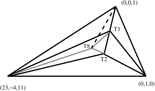
Figure 5: ${\mathbb{C}}^{3}/{\mathbb{Z}}_{23}\ (1,4,-11)$ : The three points $\alpha_{1},\alpha_{2},\alpha_{3}$ defining the affine hyperplane $\Delta$ are shown, along with the five tachyons $T_{2},T_{1},T_{8}$ in Type II. The solid lines show the subdivisions corresponding to the sequence of most relevant tachyons while the dotted lines show some possible flips.

The vertices of the affine hyperplane of marginal operators are $\alpha_{1}=(23,-4,11),\ \alpha_{2}=(0,1,0),\ \alpha_{3}=(0,0,1)$ while the tachyons correspond to the lattice vectors $T_{1}=(1,0,1),\ T_{2}=(2,0,1),\ T_{8}=(8,-1,4)$.  $T_{1}$ and $T_{2}$ are coplanar with $\alpha_{3}$. The volumes of some subcones are

$${}V(\alpha_{1},\alpha_{2},T_{8})=V(\alpha_{1},T_{2},T_{1})=V(\alpha_{3},\alpha_{1},T_{1})=4,\ \ V(\alpha_{2},\alpha_{3},T_{2})=2,\ \ V(\alpha_{1},T_{2},T_{8})=1,$$

$${}V(\alpha_{3},T_{1},T_{8})=V(\alpha_{2},\alpha_{3},T_{1})=V(\alpha_{2},T_{1},T_{2})=V(T_{1},T_{2},T_{8})=V(\alpha_{1},\alpha_{2},T_{2})=1,\$$

$${}V(\alpha_{2},T_{2},T_{8})=0,\ \ V(\alpha_{2},\alpha_{3},T_{8})=V(\alpha_{3},\alpha_{1},T_{2})=8,\ \ V(\alpha_{3},\alpha_{1},T_{8})=9.$$ (83)

As before let us analyze the sequence of most relevant tachyons, i.e. $T_{2},T_{1},T_{8}$. Condensation of $T_{2}$ gives the residual subcones $C(0;\alpha_{1},\alpha_{2},T_{2}),\ C(0;T_{2},\alpha_{2},\alpha_{3}),\ C(0;T_{2},\alpha_{3},\alpha_{1})$, which correspond to flat space, ${\mathbb{Z}}_{2}\ (1,0,-1)$ and ${\mathbb{Z}}_{8}\ (23,-1,-2)\equiv{\mathbb{Z}}_{8}\ (1,1,2)$ singularities respectively, using the Smith normal form: alternatively this can be seen by realizing the combinations  ${1\over 2}(T_{2}-\alpha_{3})=(1,0,0)$ and  ${1\over 8}(23T_{2}-\alpha_{3}-2\alpha_{1})=(0,1,0)$ of the lattice vectors (shifting by integer multiples thereof). Since $\ T_{1}={1\over 2}(T_{2}+\alpha_{3})$, it is clear that $T_{1}$ is marginal after condensation of $T_{2}$. It is straightforward to work out the twisted states of these residual orbifolds and map $T_{1}$ onto the corresponding new twisted sector (it is important however to be careful in finding the correct Type II projection for the residual orbifolds which is consistent with the original theory). On the other hand, the subsequent tachyon $T_{8}$ with renormalized R-charge

$$R_{8}^{\prime}=\ell_{\Delta^{31T}}(T_{8})={D^{31T}(T_{8})\over D^{31T}(T_{2})}={21\over 23}\ \biggl{[}\ 1+{9\over 8}\ {1-{11\over 23}\over{21\over 23}}\ \biggr{]}={3\over 2}>1$$ (84)

has become irrelevant after $T_{2}$ condenses! In fact, we have  $T_{8}={9\over 8}T_{2}+{1\over 4}\alpha_{1}+{1\over 8}\alpha_{3}$,  i.e. one of the coefficients is greater than unity. In figure 5, the solid lines correspond to the sequence of most relevant tachyons, while the lightly shaded lines correspond to the subdivision by the now irrelevant $T_{8}$. The total volume of the subcones with this sequence of subdivisions is $V_{total}=8+2+1=11$. We can now only subdivide by the remaining now-marginal operator $T_{1}$ since $T_{8}$ being irrelevant does not affect the conformal field theory. Realizing the lattice vector combinations  ${1\over 4}(23T_{1}-16\alpha_{3}-\alpha_{1})=(0,1,0)$  and  ${1\over 4}(24T_{2}-2T_{1}-2\alpha_{1})=(0,1,0)$, we see that the $T_{1}$ subdivision results in the subcones $C(0;T_{1},\alpha_{3},\alpha_{1})$ and $C(0;T_{2},T_{1},\alpha_{1})$, which are respectively ${\mathbb{Z}}_{4}\ (1,0,1)$ and ${\mathbb{Z}}_{4}\ (0,1,1)$ geometric terminal singularities (since the potential tachyons do not survive the Type II GSO projection). However we must realize that both of these are secretly supersymmetric ${\mathbb{Z}}_{4}\ (1,-1)$ singularities when twisted states in the other (anti-)chiral rings are taken into account. Thus the final endpoint of the most-relevant-tachyon sequence in this Type II theory includes only flat and supersymmetric spaces.

On the other hand, note that there are flip transitions (shown by the dotted lines) if $T_{8}$ condenses first followed by $T_{2},T_{1}$, landing up at distinct endpoints via condensation of different sequences of tachyons. Since $T_{2}={1\over 4}(T_{8}+\alpha_{2})$, $T_{2}$ remains relevant with renormalized R-charge ${1\over 2}$ after $T_{8}$ has condensed. The subsequent tachyon $T_{1}$ has renormalized R-charge

$$R_{1}^{\prime}=\ell_{\Delta^{23T}}(T_{1})={D^{23T}(T_{1})\over D^{23T}(T_{8})}={17\over 23}\ \biggl{[}\ 1+{1\over 8}\ {1-{21\over 23}\over{17\over 23}}\ \biggr{]}={3\over 4}>{17\over 23}$$ (85)

The total volume of the subcones in this case is $V_{total}=9+6(1)=15>11$, which verifies the fact that the most relevant tachyon sequence gives minimal total volume for the subcones.

6 Conclusions

We have studied condensation of localized tachyons in ${\mathbb{C}}^{3}/{\mathbb{Z}}_{N}$ nonsupersymmetric orbifolds via the worldsheet RG flows induced thereby. We have seen that this generically leads to a set of decoupled residual geometries that include $geometric$ terminal singularities, with no marginal or relevant Kähler blowups by which they can be resolved (although generic metric blowup modes generically do exist). Treated as geometric spaces, they thus admit no canonical resolution and the various possible distinct resolutions via condensation of distinct sequences of tachyons are sometimes related by flip transitions. In general, the renormalized R-charges of subsequent tachyons in the residual geometries are higher than their previous values. Thus the residual geometries in general are more prone to becoming terminal singularities after tachyon condensation. For Type II theories with no bulk tachyon, we have shown that all-ring terminal singularities cannot exist, which shows that the endpoint of tachyon condensation in Type II unstable ${\mathbb{C}}^{3}/{\mathbb{Z}}_{N}$ orbifold theories are always smooth spaces.

The calculations via toric geometry described in this paper are essentially a reflection of the physics underlying gauged linear sigma models. In particular, topological twisted GLSMs may be reliably used to study tachyon condensation not simply at the endpoints of but $all$ $along$ the worldsheet RG flow and map out the phase structure of two dimensional theories including tachyons.

The methods we have used here are of course not powerful enough to study situations where, for instance, mixed tachyons (combinations of tachyons from distinct rings) condense simultaneously. In such cases, we lose control over the system because $(2,2)$ worldsheet supersymmetry breaks down.

We now make a few brief comments on the physics seen by the worldvolume theory on a D-brane probe of a nonsupersymmetric orbifold. In general, closed string twist fields appear as Fayet-Iliopoulos D-term couplings in the D-brane probe theory [32, 3, 5]. Here, the closed string twist fields that are tachyonic condense in time and thus have a time-dependent expectation value, say of functional form $T(t)$. Via the D-term equations, these induce time-dependent Higgs expectation values for the bifundamental link fields of the quiver, which are then proportional to $\sqrt{T(t)}$. For simplicity, let us assume that closed string tachyon condensation occurs so as to monotonically increase the condensate value $T(t)$. Then the link field expectation values also increase in time. Consider a low energy observer on a D-brane probe who observes physics at energy $E$. Then the link field vevs increase monotonically in time so that the link fields are naturally integrated out in time from the point of view of the low energy observer, thereby leaving a residual quiver with fewer link fields and a less singular [3] orbifold.

It would be interesting to analyze the worldvolume D-brane gauge theories on ${\mathbb{C}}^{3}/{\mathbb{Z}}_{N}$ orbifold singularities and study their implications, in part with a view to constructing stable nonsupersymmetric string vacua.

Acknowledgments: It is a pleasure to thank P. Argyres, J. Maldacena, S. Minwalla, J. Polchinski and especially P. Aspinwall and E. Martinec for helpful discussions. KN thanks the organizers of the KITP Superstring Cosmology conference, Santa Barbara, USA and the IIT Kanpur String Workshop, Kanpur, India for hospitality during some stages of this work. This material is based upon work supported by the National Science Foundation under Grant Nos. PHY99-07949 and DMS-0074072.

Appendix A The GSO projection

Our discussion of the chiral GSO is based on and generalizes that appearing in [11, 12, 3, 4, 5, 2, 13]. We first outline a method to engineer the GSO projection based essentially on its action on the untwisted sector and consistency thereof with supersymmetric orbifolds. Then we work out the RNS partition function and, by requiring modular invariance thereof, obtain the GSO projection.

“Engineering” the GSO projection
Here we outline a method to engineer the chiral GSO projection for a Type II orbifold ${\mathbb{C}}^{3}/{\mathbb{Z}}_{N}\ (k_{1},k_{2},k_{3})$ with $k_{i}$ not necessarily equal to one. We complexify the eight transverse untwisted fermions into $\psi_{i}=e^{iH_{i}},\ i=0,1,2,3$. Consider a symmetry acting on the untwisted (complex) fermions and the twist fields via $H_{i}\rightarrow H_{i}+a_{i}\pi$, i.e.

$$\psi_{i} \rightarrow \psi_{i}\ {\rm e}^{ia_{i}\pi},$$

$${}X_{j} \rightarrow X_{j}\ \ {\rm exp}\biggl{[}i\pi\sum_{i}a_{i}\biggl{\{}{jk_{i}\over N}\biggr{\}}\biggr{]}\equiv X_{j}\ (-1)^{E_{j}}.$$ (86)

This defines a $(-1)^{F_{L}}$ ${\mathbb{Z}}_{2}$ action on the untwisted sector thus eliminating the bulk tachyon only if the $a_{i}$ are odd integers. The action on the twisted states $X_{j}$ is a well-defined ${\mathbb{Z}}_{2}$ if the exponent $E_{j}$ is an integer. This GSO exponent can be written as

$$E_{j}=\sum_{i}a_{i}\biggl{\{}{jk_{i}\over N}\biggr{\}}={j\over N}\ \sum_{i}a_{i}k_{i}-\sum_{i}a_{i}\biggl{[}{jk_{i}\over N}\biggr{]}.$$ (87)

Thus $E_{j}$ is integral if we have $a_{i}=odd$ satisfying $\ \sum_{i}a_{i}k_{i}=0\ ({\rm mod\ 2N})$. Consider the case $\sum_{i}k_{i}=odd$. Then

$$\sum a_{i}k_{i}=a_{1}k_{1}+a_{2}k_{2}+a_{3}({\rm odd}-k_{1}-k_{2})=(a_{1}-a_{3})k_{1}+(a_{2}-a_{3})k_{2}+{\rm odd}={\rm odd}$$ (88)

since the first two terms (containing differences of two odd integers) are each even. Thus this shows that no $a_{i}=odd$ exist satisfying $\ \sum_{i}a_{i}k_{i}=0\ ({\rm mod\ 2N})$: in other words, for even $N$ and $\sum_{i}k_{i}=odd$, no chiral GSO projection exists (note that for odd $N$, one can always shift say $k_{3}\rightarrow k_{3}\pm N$ to make $\sum_{i}k_{i}$ even and thereby recover a chiral GSO projection).

For $\sum_{i}k_{i}=even$, $E_{j}$ simplifies to

$$E_{j}=\sum_{i}a_{i}\biggl{[}{jk_{i}\over N}\biggr{]} = \sum_{i}\biggl{[}{jk_{i}\over N}\biggr{]}+{\rm even}$$

$$= {j\over N}\sum_{i}k_{i}-R_{j}+{\rm even},$$

where $R_{j}=\sum_{i}\{{jk_{i}\over N}\}$ is the R-charge of the twisted state. Thus for a twisted state $T$ with R-charge $R=(r_{1},r_{2},r_{3})$ in the orbifold ${\mathbb{C}}^{3}/{\mathbb{Z}}_{N}\ (k_{1},k_{2},k_{3})$, the GSO exponent is

$$E=\sum_{i}a_{i}r_{i},\qquad{\rm with}\ \ a_{i}={\rm odd\ and}\ \sum a_{i}k_{i}=0\ ({\rm mod}2N).$$ (90)

Let us examine this GSO exponent in greater detail to elucidate its properties.

For ${\mathbb{C}}/{\mathbb{Z}}_{N}$, consider the action $H\rightarrow H+a\pi$, i.e.

$$\psi\rightarrow\psi\ (-1)^{a},\qquad\qquad X_{j}\rightarrow X_{j}\ (-1)^{ja/N},$$ (91)

which defines a nontrivial $(-1)^{F_{L}}$ ${\mathbb{Z}}_{2}$ action on the untwisted sector only if $a$ is an odd integer. For odd $N=2M+1$ prime and general odd $a=2b+1$, the action on the twisted states $X_{j}$ defines a ${\mathbb{Z}}_{2}$ only if $a=N$. For other odd $N$, there are appropriate twist-$j$ subsectors with prime factors for which the argument is then the same. Indeed let us consider even $N=2^{k}$ with $a=2b+1$, so that the twisted states transform as

$$X_{j}\rightarrow X_{j}\ (-1)^{ja/N}=X_{j}\ (-1)^{j(2b+1)/(2^{k})}$$ (92)

Then for no twist-$j$ subsector is there a well-defined ${\mathbb{Z}}_{2}$. For general even N=2M, there are twist-j subsectors which are identical to the above cases. Thus we take $a=N$ with $N$ odd for Type II ${\mathbb{C}}/{\mathbb{Z}}_{N}$. Then the chiral GSO above acts as

$$\psi\rightarrow\psi\ (-1)^{N},\qquad\qquad X_{j}\rightarrow X_{j}\ (-1)^{j}.$$ (93)

Since the $(-1,-1)$ picture vertex operators are odd under chiral GSO, only the $X_{j}$ states with odd $j$ survive.

Now consider ${\mathbb{C}}^{2}/{\mathbb{Z}}_{N(p)}$ and ${\mathbb{C}}^{3}/{\mathbb{Z}}_{N(p,q)}$. In these cases, the GSO exponent $E_{j}$ is an integer if $\ a_{1}+a_{2}p+a_{3}q=0({\rm mod\ 2N})$.

From above, we have $\ 1+p+q=even$. For ${\mathbb{C}}^{2}/{\mathbb{Z}}_{N(p)}$, we have $q=0$: then $p=odd$ and $a_{1}=p,a_{2}=-1$ satisfy $\ a_{1}+a_{2}p=0\ ({\rm mod}2N)$. We have then the chiral GSO action

$$\psi_{1}\rightarrow\psi_{1}\ (-1)^{p},\ \ \psi_{2}\rightarrow\psi_{2}\ (-1),\qquad\qquad X_{j}\rightarrow X_{j}\ (-1)^{[jp/N]}$$ (94)

for the ${\mathbb{C}}^{2}/{\mathbb{Z}}_{N(p)}$ orbifold.

Note that the supersymmetric orbifold is $p=-1$ in this convention, so that $[{jp\over N}]=[-{j\over N}]=-1$. Thus the chiral GSO acts as $X_{j}\rightarrow X_{j}(-1)$ for all twisted states, which in fact are marginal with R-charge $R_{j}={j\over N}+\{-{j\over N}\}=1$. Thus the entire $(c_{X},c_{Y})$ ring is preserved by the chiral GSO in this case, while the entire $(c_{X},a_{Y})$ ring is projected out.

For ${\mathbb{C}}^{3}/{\mathbb{Z}}_{N(p,q)}$, we have $p+q=odd$: then $a_{1}=p+q,a_{2}=a_{3}=-1$ satisfy $\ a_{1}+a_{2}p+a_{3}q=0({\rm mod\ 2N})$. Then the GSO exponent $E_{j}$ is

$$E_{j}=\biggl{[}{jp\over N}\biggr{]}+\biggl{[}{jq\over N}\biggr{]}={j\over N}\ (1+p+q)-{j\over N}-\biggl{\{}{jp\over N}\biggr{\}}-\biggl{\{}{jq\over N}\biggr{\}}={j\over N}\ (1+p+q)-R_{j}.$$ (95)

and we have the chiral GSO action

$$\psi_{1}\rightarrow\psi_{1}\ (-1)^{p+q},\ \ \psi_{2}\rightarrow\psi_{2}\ (-1),\ \ \psi_{3}\rightarrow\psi_{3}\ (-1),\qquad X_{j}\rightarrow X_{j}\ (-1)^{[jp/N]+[jq/N]}.$$ (96)

For the supersymmetric case $1+p+q=0$ and we have $\ E=-R_{j}\$, so that the chiral GSO acts as $X_{j}\rightarrow X_{j}(-1)$ for all twisted states in the $(c_{X},c_{Y},c_{Z})$ ring with R-charge $R_{j}=1$. The blowup modes of the geometry are defined purely in terms of the marginal $R_{j}=1$ states for the supersymmetric case so that they are all preserved by the GSO (note that there also exist $R_{j}=2$ twisted states here, unlike in the ${\mathbb{C}}^{2}/{\mathbb{Z}}_{N(p)}$ case). Thus in general, the chiral GSO for Type II theories projects out the twist operators $X_{j}$ of the $(c_{X},c_{Y},c_{Z})$ ring with $[{jp\over N}]+[{jq\over N}]\in 2{\mathbb{Z}}$ and retains those with either $[{jp\over N}]$ or $[{jq\over N}]$ odd (but not both). Similarly in the $(c_{X},c_{Y},a_{Z})$ ring, the $X_{j}$ with $[{jp\over N}]+[{jq\over N}]$ even are retained and so on.

Note that this agrees with the Green-Schwarz GSO analysis (generalized from that in [3]), which starts with a rotation generator

$$R={\rm exp}\biggl{[}{2\pi i\over N}(J_{45}+pJ_{67}+qJ_{89})\biggr{]}$$ (97)

Then

$$R^{N}=(-1)^{2(s_{45}+ps_{67}+qs_{89})}$$ (98)

so that considering the action thereof on various spinor charge sectors $(\pm 1/2,\pm 1/2,\pm 1/2)$, and demanding $R^{N}=1$ for removing the bulk tachyon gives $p+q=odd$.

It is important to note that changing $q\rightarrow q+N$ introduces an extra factor of $(-1)^{N}$ in (96). Also $p+q=odd$ now changes to $p+q+N=even$ thus reversing the bulk tachyon projection and changing a Type II theory to Type 0. For example, the ${\mathbb{C}}^{3}/{\mathbb{Z}}_{11(2,-7)}$ orbifold is a good Type II theory with the bulk tachyon projected out, whereas the orbifold ${\mathbb{C}}^{3}/{\mathbb{Z}}_{11(2,4)}$ (which is equivalent in conformal field theory) does have a bulk tachyon and should be regarded as Type 0. Furthermore, the action on the twisted states changes since the exponent $E$ becomes $E\rightarrow j+E$, so that supersymmetric orbifolds now have $E\rightarrow{j\over N}(1+p+q+N)-R_{j}=j-R_{j}$, thus projecting down to $j=even$ twisted states among the $R_{j}=1$ blowup modes.

Modular invariance of the partition function
The partition function for ${\mathbb{C}}/{\mathbb{Z}}_{N}$ was described notably in [11, 12], using both the Green-Schwarz and the RNS formulations. We primarily use the RNS formulation here.

The Type 0 string has a diagonal GSO projection that ties together the left and right movers: it has the partition function

$$Z = {1\over 2N}\sum_{j,l=0}^{N-1}\ {1\over|\eta^{2}(\tau){\bar{\eta}}^{2}({\bar{\tau}})|}\ \prod_{i=1}^{3}\ \Biggl{|}{\eta(\tau)\over\theta[{\begin{array}[]{c}{1\over 2}+jk_{i}/N\\ {1\over 2}+lk_{i}/N\\ \end{array}}](0,\tau)}\Biggr{|}^{2}\cdot\qquad\qquad$$ (101)

$${}\Biggl{[}\ \ \biggl{|}\prod_{i=1}^{3}\theta\left[{\begin{array}[]{c}{jk_{i}\over N}\\ {lk_{i}\over N}\\ \end{array}}\right]\ \theta\left[{\begin{array}[]{c}0\\ 0\\ \end{array}}\right]\biggr{|}^{2}+\biggl{|}\prod_{i=1}^{3}\theta\left[{\begin{array}[]{c}{jk_{i}\over N}\\ {lk_{i}\over N}+{1\over 2}\\ \end{array}}\right]\ \theta\left[{\begin{array}[]{c}0\\ {1\over 2}\\ \end{array}}\right]\biggr{|}^{2}$$ (110)

$${}+\biggl{|}\prod_{i=1}^{3}\theta\left[{\begin{array}[]{c}{jk_{i}\over N}+{1\over 2}\\ {lk_{i}\over N}\\ \end{array}}\right]\ \theta\left[{\begin{array}[]{c}{1\over 2}\\ 0\\ \end{array}}\right]\biggr{|}^{2}\pm\biggl{|}\prod_{i=1}^{3}\theta\left[{\begin{array}[]{c}{jk_{i}\over N}+{1\over 2}\\ {lk_{i}\over N}+{1\over 2}\\ \end{array}}\right]\ \theta\left[{\begin{array}[]{c}{1\over 2}\\ {1\over 2}\\ \end{array}}\right]\biggr{|}^{2}\ \ \Biggr{]}$$ (119)

Clearly this partition function exists for any $k_{i},N$.

On the other hand, the 1-loop partition function on a ${\mathbb{C}}^{3}/{\mathbb{Z}}_{N}\ (k_{1},k_{2},k_{3})$ orbifold for a Type II string with separate GSO projections on the left and right movers is given by the sum over twisted sectors as

$$Z={1\over 4N}\sum_{j,l=0}^{N-1}\ {1\over|\eta^{2}(\tau){\bar{\eta}}^{2}({\bar{\tau}})|}\ \prod_{i=1}^{3}\ \Biggl{|}{\eta(\tau)\over\theta[{\begin{array}[]{c}{1\over 2}+jk_{i}/N\\ {1\over 2}+lk_{i}/N\\ \end{array}}](0,\tau)}\Biggr{|}^{2}\ \biggl{|}{\zeta^{j}_{l}\over|\eta^{4}(\tau)}\biggr{|}^{2}$$ (120)

where

$$\zeta^{j}_{l} = \prod_{i=1}^{3}\theta\left[{\begin{array}[]{c}{jk_{i}\over N}\\ {lk_{i}\over N}\\ \end{array}}\right]\ \theta\left[{\begin{array}[]{c}0\\ 0\\ \end{array}}\right]-e^{-i\pi\sum_{i}{jk_{i}\over N}}\prod_{i=1}^{3}\theta\left[{\begin{array}[]{c}{jk_{i}\over N}\\ {lk_{i}\over N}+{1\over 2}\\ \end{array}}\right]\ \theta\left[{\begin{array}[]{c}0\\ {1\over 2}\\ \end{array}}\right]$$ (129)

$${}-\prod_{i=1}^{3}\theta\left[{\begin{array}[]{c}{jk_{i}\over N}+{1\over 2}\\ {lk_{i}\over N}\\ \end{array}}\right]\ \theta\left[{\begin{array}[]{c}{1\over 2}\\ 0\\ \end{array}}\right]-e^{-i\pi\sum_{i}{jk_{i}\over N}}\prod_{i=1}^{3}\theta\left[{\begin{array}[]{c}{jk_{i}\over N}+{1\over 2}\\ {lk_{i}\over N}+{1\over 2}\\ \end{array}}\right]\ \theta\left[{\begin{array}[]{c}{1\over 2}\\ {1\over 2}\\ \end{array}}\right]$$ (138)

contains the sum over spin structures for the j-th twisted sector twisted by $g^{l}$ in the “time” direction. The terms in Z are easily recognized as the contributions from the untwisted bosons in the one complex flat dimension, multiplied by the contributions from the twisted bosons in the three orbifolded complex dimensions and the fermionic contributions.

At this point, we list some formulae involving theta functions that we use here (from [11, 35]). The boundary conditions on the worldsheet scalars and spinors in the NS sector are

$$X(w+2\pi) = e^{2\pi ia}X(w),\qquad X(w+2\pi\tau)=e^{2\pi ib}X(w),$$

$$\psi(w+2\pi) = -e^{2\pi ia}\psi(w)\equiv-e^{-i\pi\alpha}\psi(w),$$

$$\psi(w+2\pi\tau) = -e^{2\pi ib}\psi(w)\equiv-e^{-i\pi\beta}\psi(w).$$ (139)

A chiral fermion with Hamiltonian

$$H_{a}=\sum_{n=1}^{\infty}\biggl{[}(n-{1\over 2}+a)d^{{\dagger}}_{n}d_{n}+(n-{1\over 2}-a){\bar{d}}^{{\dagger}}_{n}{\bar{d}}_{n}\biggr{]}+{a^{2}\over 2}-{1\over 24}$$ (140)

has the partition function

$$Z^{\alpha}_{\beta} = Tr\ (h_{b}q^{H_{a}})={\theta[{\begin{array}[]{c}a\\ b\\ \end{array}}]\over\eta(\tau)}\equiv{\theta[{\begin{array}[]{c}-{\alpha\over 2}\\ -{\beta\over 2}\\ \end{array}}]\over\eta(\tau)}$$ (145)

$$= e^{2\pi iab}\ q^{{a^{2}\over 2}-{1\over 24}}\ \prod_{n=1}^{\infty}(1+q^{n-{1\over 2}+a}\ e^{2\pi ib})(1+q^{n-{1\over 2}-a}\ e^{-2\pi ib})$$ (146)

where the ${\mathbb{Z}}_{N}$ action on the Hilbert space is

$$h_{b}dh_{b}^{-1}=-e^{-2\pi ib}d,\qquad{\bar{h}}_{b}{\bar{d}}{\bar{h}}_{b}^{-1}=-e^{2\pi ib}{\bar{d}}$$ (147)

Some useful formulae involving theta functions are

$$\theta[{\begin{array}[]{c}a\\ b\\ \end{array}}](\nu,\tau)=e^{i\pi a^{2}\tau+2\pi ia(\nu+b)}\ \theta[{\begin{array}[]{c}0\\ 0\\ \end{array}}](\nu+a\tau+b,\tau)=\sum_{n\in{\mathbb{Z}}}q^{{1\over 2}(n+a)^{2}}\ e^{2\pi i(n+a)(\nu+b)}$$ (152)

$${}\theta[{\begin{array}[]{c}a+r\\ b+s\\ \end{array}}](\nu,\tau)=e^{i\pi isa}\theta[{\begin{array}[]{c}a\\ b\\ \end{array}}](\nu,\tau),\qquad r,s\in{\mathbb{Z}}$$ (157)

Under modular transformations generated by $S:\tau\rightarrow-{1\over\tau}$ and $T:\tau\rightarrow\tau+1$, we have

$$T:\ \theta[{\begin{array}[]{c}a\\ b\\ \end{array}}]\rightarrow e^{-i\pi a^{2}-i\pi a}\ \theta[{\begin{array}[]{c}a\\ a+b+{1\over 2}\\ \end{array}}],\qquad\eta\rightarrow e^{i\pi/12}\ \eta$$ (162)

$${}S:\ \theta[{\begin{array}[]{c}a\\ b\\ \end{array}}]\rightarrow(-i\tau)^{1\over 2}e^{2\pi iab}\ \theta[{\begin{array}[]{c}-b\\ a\\ \end{array}}],\qquad\eta\rightarrow(-i\tau)^{1\over 2}\eta$$ (167)

Thus under an S-transformation, we have

$${\zeta^{j}_{l}\over\eta^{4}} \rightarrow e^{2\pi i\sum_{i}{jlk_{i}^{2}\over N^{2}}}\Biggl{\{}\prod_{i=1}^{3}\theta\left[{\begin{array}[]{c}-{lk_{i}\over N}\\ {jk_{i}\over N}\\ \end{array}}\right]\ \theta\left[{\begin{array}[]{c}0\\ 0\\ \end{array}}\right]-e^{-i\pi\sum_{i}{jk_{i}\over N}+2\pi i\sum_{i}{1\over 2}{jk_{i}\over N}}\prod_{i=1}^{3}\theta\left[{\begin{array}[]{c}-{lk_{i}\over N}-{1\over 2}\\ {jk_{i}\over N}\\ \end{array}}\right]\theta\left[{\begin{array}[]{c}-{1\over 2}\\ 0\\ \end{array}}\right]$$ (176)

$${}-e^{2\pi i\sum_{i}{1\over 2}{lk_{i}\over N}}\prod_{i=1}^{3}\theta\left[{\begin{array}[]{c}-{lk_{i}\over N}\\ {jk_{i}\over N}+{1\over 2}\\ \end{array}}\right]\ \theta\left[{\begin{array}[]{c}0\\ {1\over 2}\\ \end{array}}\right]$$ (181)

$${}-e^{-i\pi\sum_{i}{jk_{i}\over N}+2\pi i\sum_{i}{1\over 2}({jk_{i}\over N}+{lk_{i}\over N})+2\pi i({3\over 4}+{1\over 4})}\prod_{i=1}^{3}\theta\left[{\begin{array}[]{c}-{lk_{i}\over N}-{1\over 2}\\ {jk_{i}\over N}+{1\over 2}\\ \end{array}}\right]\ \theta\left[{\begin{array}[]{c}-{1\over 2}\\ {1\over 2}\\ \end{array}}\right]\Biggr{\}}\ .$$ (186)

The sum over such terms can be rewritten as the original partition function with $j^{\prime}=N-l,\ l^{\prime}=j$ if the phase from the third term above satisfies

$$e^{i\pi\sum_{i}{lk_{i}\over N}}=e^{-i\pi\sum_{i}{j^{\prime}k_{i}\over N}}=e^{-i\pi\sum_{i}{(N-l)k_{i}\over N}}$$ (187)

In other words, we require

$$\sum_{i}{(N-l)k_{i}\over N}=-\sum_{i}{lk_{i}\over N}+{\rm even}$$ (188)

i.e. $\sum_{i}k_{i}=$ even, the condition we have seen before (this condition on the orbifold weights can also be obtained by demanding level-matching). Invariance under the T transformation does not give anything new.

We can now expand the Type II partition function we have here to realize the GSO projection on the twisted states to obtain the projector

$$1-(-1)^{-i\pi\sum_{i}[jk_{i}/N]}$$ (189)

for the ground states in the sector where $\{{jk_{i}\over N}\}<{1\over 2}$, i.e. the $(c_{X},c_{Y},c_{Z})$ ring. This is a projector onto twisted states with  $\sum_{i}[jk_{i}/N]=E_{j}=odd$, recovering the result from the previous subsection. On the other hand, consider as an example, the sector where $\{{jk_{3}\over N}\}>{1\over 2}$ with $\{{jk_{1}\over N}\},\{{jk_{2}\over N}\}<{1\over 2}$. Then we obtain the projector

$$1-(-1)^{-i\pi(\sum_{i}[jk_{i}/N]-1)}$$ (190)

for the ground states (which are in the $(c_{X},c_{Y},a_{Z})$ ring), i.e. $\sum_{i}[jk_{i}/N]=even$. The chiral operators $X_{j}$ are obtained as the excited state with one extra fermion number from $\psi_{3}$ which therefore have the GSO projection $\sum_{i}[jk_{i}/N]=E_{j}=odd$, as before. Likewise if two of $\{{jk_{i}\over N}\}>{1\over 2}$, we have $E_{j}=odd$ for the ground states so that the $X_{j}$, obtained with one extra fermion number in the two sectors, again have $E_{j}=odd$ and so on. Thus the GSO exponent for the chiral operators $X_{j}$ is $E_{j}=\sum_{i}[jk_{i}/N]=odd$.

The above partition function can be recast as the Green-Schwarz partition function using the quartic Riemann identity for theta functions [13] (see [11, 12] for the ${\mathbb{C}}/{\mathbb{Z}}_{N}$ case). It is noteworthy that the partition function of the Type II theory can be obtained by gauging a chiral $(-1)^{F_{L}}$ ${\mathbb{Z}}_{2}$ symmetry in (i.e. as a ${\mathbb{Z}}_{2}$ orbifold of) the partition function of the Type 0 theory and demanding modular invariance, along the lines of [36, 37]. In this case, this procedure effectively changes the ${\mathbb{Z}}_{N}$ orbifold to a ${\mathbb{Z}}_{N}\times{\mathbb{Z}}_{2}$. For odd $N$, this is the same as ${\mathbb{Z}}_{2N}$ and we recover the partition function above and thence the Green-Schwarz partition function. While in principle one could expect interesting generalizations involving discrete torsion in ${\mathbb{Z}}_{N}\times{\mathbb{Z}}_{2}$ for even $N$, a careful calculation shows that the possible extra phases can be absorbed via redefinitions of the orbifold weights.

Appendix B ${\mathbb{C}}^{2}/{\mathbb{Z}}_{N(p)}$ toric geometry

We outline here the toric description of ${\mathbb{C}}^{2}/{\mathbb{Z}}_{N(p)}$ discussed in [5] (see also [2]), based on the Hirzebruch-Jung theory of singularity resolution in codimension two. We have uniformized our notations and conventions with our description of ${\mathbb{C}}^{3}/{\mathbb{Z}}_{N(p,q)}$.

A basis for monomials invariant under the orbifold action is $\ u=x^{N},\ v=x^{-p}y$,  so that the ring of holomorphic functions on a neighbourhood of the noncompact ${\mathbb{C}}^{2}/{\mathbb{Z}}_{N}$ singularity is generated by the monomials $\ u^{m_{1}}v^{m_{2}}=x^{Nm_{1}-pm_{2}}\ y^{m_{2}}\$ for integer $m_{1},m_{2}$, which gives a cone in the ${\mathbb{M}}$ lattice bounded by $(1,0),\ (p,N)\$. From these, we read off the vertices of the fan in the ${\mathbb{N}}$ lattice dual to this

$$\alpha_{1}=(N,-p),\qquad\alpha_{2}=(0,1).$$ (191)

This uniformizes our notations and conventions with those of [5]: see e.g. Figure 2 therein (see also e.g. Figure 1.10 of [2]). The Hirzebruch-Jung formulation of minimal resolution in codimension two ensures that the endpoint of condensation of all tachyons in a given orbifold is always flat space. Thus the volume of any subcone arising from a subdivision by a tachyonic blowup mode is equal to one, so that unlike ${\mathbb{C}}^{3}/{\mathbb{Z}}_{N(p,q)}$, terminal singularities do not exist here.

Furthermore there is a nice continued fraction representation of ${N\over p}$ for ${\mathbb{C}}^{2}/{\mathbb{Z}}_{N(p)}$, in terms of integers $a_{k}$, following from the Hirzebruch-Jung theory of minimal resolution of these orbifolds which encodes the relations

$$a_{j}v_{j}=v_{j-1}+v_{j+1}$$ (192)

between the vectors $v_{0}=(N,-p),\ v_{r+1}=(0,1),\ v_{j},\ j=1,\ldots,r$ in the toric diagram representing the bounding vectors of the fan as well as the $r$ generators of the chiral ring. Then by iterating the relation above, we can see from the toric diagram that $v_{k}$ obeys

$$A_{k}v_{k}=B_{k}v_{0}+v_{k+1},$$ (193)

where

$$A_{k}=a_{k}-1/(a_{k-1}-...),\ \ A_{1}=a_{1},\ \qquad B_{k}=[A_{k-1}.A_{k-2}...A_{1}]^{-1}.$$ (194)

Then, realizing that (1,0) is an interior point for $p<N$, we have for $v_{r}=(1,0)$,

$$A_{r}(1,0)=B_{r}(N,-p)+(0,1)$$ (195)

so that $\ A_{r}=B_{r}N,\ 1=B_{r}p$,  giving

$${N\over p}=A_{r}=[a_{r},a_{r-1}\ldots].$$ (196)

There does not appear to be any generalization of the continued fraction fraction representation for ${\mathbb{C}}^{3}/{\mathbb{Z}}_{N(p,q)}$.

In this case also, one can study subsequent tachyons Type II theories in light of the chiral GSO projection. For a ${\mathbb{C}}^{2}/{\mathbb{Z}}_{N(p)}$ orbifold that is Type II, we have $p=odd$. A twisted state $T_{j}=(j,-[{jp\over N}])\equiv({j\over N},\{{jp\over N}\})$ is preserved by the GSO if $[{jp\over N}]=odd$. Consider blowing up the divisor corresponding to $T_{j}$. The subcone $C(0;T_{j},\alpha_{2})$ can be easily seen to be a ${\mathbb{C}}^{2}/{\mathbb{Z}}_{j}\ (1,[{jp\over N}])$ orbifold which clearly admits a Type II projection since $1+[{jp\over N}]=even$. If $T_{k}\in C(0;T_{j},\alpha_{2})$, solving $T_{k}=aT_{j}+b\alpha_{2}$ gives

$$R_{k}^{\prime}=(a,b)=\biggl{(}{k\over j},\ \ {k\over j}\biggl{[}{jp\over N}\biggr{]}-\biggl{[}{kp\over N}\biggr{]}\biggr{)}.$$ (197)

The GSO requires $a_{i}=odd$ satisfying $a_{1}+a_{2}[{jp\over N}]=0\ ({\rm mod}2j)$, which is solved by $a_{1}=[{jp\over N}],a_{2}=-1$. Thus the GSO exponent for $T_{k}$ works out to

$$E=\biggl{[}{jp\over N}\biggr{]}{k\over j}-{k\over j}\biggl{[}{jp\over N}\biggr{]}+\biggl{[}{kp\over N}\biggr{]}=\biggl{[}{kp\over N}\biggr{]}.$$ (198)

Similarly, the subcone $C(0;T_{j},\alpha_{1})$ is seen to be a ${\mathbb{C}}^{2}/{\mathbb{Z}}_{N\{{jp\over N}\}}\ (p,-[{jp\over N}])$ orbifold (assuming nondegeneracy of the Smith normal form vector). This also clearly admits a Type II projection since $p-[{jp\over N}]=even$. A sub-twisted state $T_{k}\in C(0;T_{j},\alpha_{1})$ satisfies $T_{k}=aT_{j}+b\alpha_{1}$ giving

$$R_{k}^{\prime}=(a,b)=\biggl{(}{\{{kp\over N}\}\over\{{jp\over N}\}},\ \ {k\over N}-{j\over N}{\{{kp\over N}\}\over\{{jp\over N}\}}\biggr{)}.$$ (199)

A set of $a_{i}=odd$ satisfying $a_{1}p-a_{2}[{jp\over N}]=0\ ({\rm mod}2N\{{jp\over N}\})$, is $a_{1}=[{jp\over N}],a_{2}=p$, giving for the GSO exponent for $T_{k}$

$$E=\biggl{[}{kp\over N}\biggr{]}.$$ (200)

Thus originally preserved sub-twisted states remain preserved after a preserved twisted state condenses. The R-charges of subsequent tachyons again expectedly renormalize upwards, i.e. $R_{k}^{\prime}>R_{k}$, since a sub-tachyon is closer to a sub-plane than to the original plane of marginal operators. However due to an interesting convexity property of the tachyonic generators (that appear in the Hirzebruch-Jung continued fraction) inside a given cone of a toric digram (see e.g. [7]), it is straightforward to show that $R_{k}^{\prime}\leq 1$ always! Thus there are no geometric terminal singularities in codimension two.

References

- [1] See, e.g., A. Sen, “Non-BPS states and branes in string theory”, [hep-th/9904207]; L. Rastelli, A. Sen, B. Zwiebach, “Vacuum string field theory”, [hep-th/0106010], and references therein.
- [2] E. Martinec, “Defects, decay and dissipated states”, [hep-th/0210231].
- [3] A. Adams, J. Polchinski, E. Silverstein, “Don’t panic! Closed string tachyons in ALE spacetimes”, [hep-th/0108075].
- [4] C. Vafa, “Mirror symmetry and closed string tachyon condensation”, [hep-th/0111051].
- [5] J. Harvey, D. Kutasov, E. Martinec, G. Moore, “Localized tachyons and RG flows” [hep-th/0111154] ;
- [6] M. Headrick, S. Minwalla, T. Takayanagi, “Closed string tachyon condensation: an overview”, [hep-th/0405064].
- [7] E. Martinec, G. Moore, “On decay of K-theory”, [hep-th/0212059].
- [8] H. Hironaka, “Resolution of singularities of an algebraic variety over a field of characteristic zero. I, II,” Ann. of Math. (2) 79, 109 (1964).
- [9] P. S. Aspinwall, D. R. Morrison, “Stable singularities in string theory,” [hep-th/9503208].
- [10] S.-J. Sin, “Comments on the fate of unstable orbifolds”, [hep-th/0308028].
- [11] A. Dabholkar, “Strings on a cone and black hole entropy”, [hep-th/9408098], “Quantum corrections to black hole entropy in string theory”, [hep-th/9409158].
- [12] D. Lowe, A. Strominger, “Strings near a Rindler or black hole horizon”, [hep-th/9410215].
- [13] S. Lee, S.-J. Sin, “Chiral rings and GSO projection in orbifolds”, [hep-th/0308029].
- [14] S. Lee, S.-J. Sin, “Localized tachyon condensation and G parity conservation”, [hep-th/ 0312175].
- [15] L. Dixon, D. Friedan, E. Martinec, S. Shenker, “The conformal field theory of orbifolds”, Nucl. Phys. B282, 13 (1987).
- [16] E. Witten, “Phases of theories in two dimensions”, [hep-th/9301042].
- [17] D. R. Morrison, M. R. Plesser, “Summing the instantons: quantum cohomology and mirror symmetry in toric varieties”, [hep-th/9412236].
- [18] See e.g. the Foreword of “Explicit birational geometry of 3-folds”, Edited by Alessio Corti, Miles Reid, Cambridge University Press 2000, as well as articles therein.
- [19] P. S. Aspinwall, B. R. Greene, D. R. Morrison, “Calabi–Yau moduli space, mirror manifolds and spacetime topology change in string theory” [hep-th/9309097].
- [20] P. Aspinwall, “Resolution of orbifold singularities in string theory”, [hep-th/9403123].
- [21] B. R. Greene, “String theory on Calabi-Yau manifolds”, [hep-th/9702155].
- [22] D. R. Morrison, M. R. Plesser, “Nonspherical horizons, I”, [hep-th/9810201].
- [23] W. Fulton, Introduction to Toric Varieties, Princeton University Press (1993).
- [24] S. Lang, Algebra, 3rd ed., Springer-Verlag (2002).
- [25] M. Reid, “Young person’s guide to canonical singularities,” Proc. Symp. Pure Math. 46, 345 (1987).
- [26] M. Schlessinger, “Rigidity of quotient singularities,” Invent. Math. 14, 17 (1971).
- [27] J. Fine, “On varieties isomorphic in codimension one to torus embeddings,” Duke Math. J. 58, 79 (1989).
- [28] S. Mori, “Threefolds whose canonical bundles are not numerically effective,” Ann. of Math. (2) 116, 133 (1982).
- [29] D. R. Morrison, G. Stevens, “Terminal quotient singularities in dimensions three and four,” Proc. Amer. Math. Soc. 90, 15 (1984).
- [30] S. Mori, “Flip theorem and the existence of minimal models for -folds,” J. Amer. Math. Soc. 1, 117 (1988).
- [31] V. I. Danilov, “Birational geometry of three-dimensional toric varieties,” Math. USSR Ivz. 21, 269 (1983).
- [32] M. Douglas, G. Moore, “D-branes, quivers and ALE instantons”, [hep-th/9603167].
- [33] K. Narayan, “Blocking up D-branes : Matrix renormalization?” [hep-th/0211110].
- [34] K. Narayan, M. R. Plesser, “Coarse-graining quivers”, [hep-th/0309171].
- [35] J. Polchinski, String Theory, Vol. 1,2. Cambridge University Press (1998).
- [36] N. Seiberg, E. Witten, “Spin structures in string theory”, Nucl. Phys. B276, 272 (1986).
- [37] L. Alvarez-Gaume, G. Moore, C. Vafa, “Theta functions, modular invariance and strings”, Comm. Math. Phys. 106, 1 (1986).