hep-th/0406038

KCL-MTH-04-07

SPIN-04/08

ITP-04/14

UG-04/02

Non-extremal D-instantons

E. Bergshoeff¹, A. Collinucci¹, U. Gran², D. Roest¹ and S. Vandoren³

¹ Centre for Theoretical Physics, University of Groningen

Nijenborgh 4, 9747 AG Groningen, The Netherlands

E-mail: (e.a.bergshoeff, a.collinucci, d.roest)@phys.rug.nl

² Department of Mathematics, King’s College London

Strand, London WC2R 2LS, United Kingdom

E-mail: ugran@mth.kcl.ac.uk

³ Institute for Theoretical Physics, Utrecht University

Leuvenlaan 4, 3508 TD Utrecht, The Netherlands

E-mail: s.vandoren@phys.uu.nl

ABSTRACT

We construct the most general non-extremal deformation of the D-instanton solution with maximal rotational symmetry. The general non-supersymmetric solution carries electric charges of the $SL(2,\mathbb{R})$ symmetry, which correspond to each of the three conjugacy classes of $SL(2,\mathbb{R})$. Our calculations naturally generalise to arbitrary dimensions and arbitrary dilaton couplings.

We show that for specific values of the dilaton coupling parameter, the non-extremal instanton solutions can be viewed as wormholes of non-extremal Reissner-Nordström black holes in one higher dimension. We extend this result by showing that for other values of the dilaton coupling parameter, the non-extremal instanton solutions can be uplifted to non-extremal non-dilatonic $p$-branes in $p+1$ dimensions higher.

Finally, we attempt to consider the solutions as instantons of (compactified) type IIB superstring theory. In particular, we derive an elegant formula for the instanton action. We conjecture that the non-extremal D-instantons can contribute to the $R^{8}$-terms in the type IIB string effective action.

PACS number: 04.50.+h 04.65.+e 11.25.-w

1 Introduction

Gravity coupled to the two scalars (dilaton and axion) that parameterise an $SL(2,\hbox{\mybb R})/SO(2)$ coset space is an important subsector of the low-energy limit of type IIB superstring theory. Among the different solutions of this system are seven-brane solutions that carry magnetic charges with respect to the three generators of $SL(2,\hbox{\mybb R})$. These magnetic charges combine into a traceless 2 x 2 charge matrix $Q_{M}$ which transforms in the adjoint representation of $SL(2,\hbox{\mybb R})$. The combination $\det(Q_{M})$, being invariant under these transformations, labels the three different conjugacy classes of $SL(2,\hbox{\mybb R})$. Each pair of solutions in the same conjugacy class is related via $SL(2,\hbox{\mybb R})$. On the other hand, two solutions that belong to two different conjugacy classes can not be related via $SL(2,\hbox{\mybb R})$.

The three classes of inequivalent seven-brane solutions, whose magnetic charges correspond to the three conjugacy classes of $SL(2,\hbox{\mybb R})$, have been constructed in [1]. All of these seven-brane solutions are half-supersymmetric. The conjugacy class with $\det(Q_{M})=0$ has $\mathbb{R}$ isometry in the transverse space and is represented by the so-called “circular” 1/2 BPS D7–brane [2]. The other two classes, with $\det(Q_{M})>0$ and $\det(Q_{M})<0$, describe seven-branes with $SO(2)$ and $SO(1,1)$ isometry in the transverse directions, respectively. Actually, there exist two solutions describing seven-branes with $SO(2)$ isometries [1] whose interpretation has become clear only recently [3]. The first solution describes a set of (positively and negatively charged) D7-branes which are distributed along a finite line-element in one of the two transverse directions. A special feature is that the total D7-brane charge vanishes. The second solution can be obtained by taking the first solution in the limit of a zero-size line-element. Since the total D7-brane charge vanishes, one is not left with a single D7-brane but, instead, one obtains a conical space-time with a specific deficit angle [3].

It is well-known that the electric-magnetic dual of the D7–brane is the D-instanton [4, 5]. The D-instanton is a half-supersymmetric solution of the Euclidean gravity-dilaton-axion system, where the dilaton and axion parameterise an $SL(2,\hbox{\mybb R})/SO(1,1)$ coset, and carries electric charge with respect to the Euclidean $SL(2,\hbox{\mybb R})$ symmetry. In complete analogy to the case of seven-branes, the three Euclidean $SL(2,\hbox{\mybb R})$ charges combine into a 2 x 2 charge matrix $Q_{E}$ that transforms in the adjoint representation of the Euclidean $SL(2,\mathbb{R})$. The D-instanton is represented by the same conjugacy class that represents the circular D7–brane, i.e. the one with $\det(Q_{E})=0$.

It is natural to ask, in analogy to the case of seven-branes discussed above, whether there exist “exotic” instantons with electric $SL(2,\hbox{\mybb R})$ charges corresponding to the other two conjugacy classes, i.e. the ones with $\det(Q_{E})>0$ and $\det(Q_{E})<0$. It is the aim of this paper to construct and investigate such solutions. For earlier work on generalised D-instanton solutions, see [6, 7, 8, 9, 10, 11, 12, 13, 14]. To be specific, in this paper we will construct solutions with maximal rotational symmetry for general values of the charge matrix $Q_{E}$, thus generalising the D–instanton, and for arbitrary dimension $D$ and dilaton coupling $b$, thus including compactifications of type IIB string theory. We will always refer to the instanton solutions in the $\det(Q_{E})=0$ conjugacy class as D-instantons, though we allow for the generalisation to arbitrary dimension and dilaton coupling.

In contrast to the D-instanton we find that solutions corresponding to the other two conjugacy classes, in Einstein frame, do not have a flat metric but rather a conformally flat metric (which is implied by the rotational $SO(D)$ symmetry). Moreover, the scalars can be expressed in terms of one rotationally symmetric function which is harmonic over the conformally flat space. Unlike the case of seven-branes, where all three conjugacy classes preserve half supersymmetry [1], we find that the generalised instantons of the other two conjugacy classes do not preserve any supersymmetry. It has been noted that the standard D-instanton has a manifest wormhole geometry in the string frame metric [4, 15]. Curiously, we find that this holds for all values of $b$ and $D$ for the $\det Q_{E}=0$ solution in string frame and the $\det Q_{E}>0$ solution in Einstein frame. In addition, for a particular value of the dilaton coupling parameter, the same applies to the other conjugacy class with $\det Q_{E}<0$ provided we use the so-called dual frame metric.

One can view the generalised instantons as non-extremal deformations of the half-supersymmetric instanton. This point of view is confirmed by the fact that a subclass of these solutions can be viewed as describing wormholes corresponding to non-extremal Reissner-Nordström black holes in one dimension higher. More generally, for specific values of the dilaton coupling parameter, the non-extremal instanton solutions can be uplifted to regular non-extremal non-dilatonic $p$-branes in $p+1$ dimensions higher.

Alternatively, we will describe in this paper an attempt to consider the non-extremal D-instantons as true (albeit non-supersymmetric) instantons of type IIB superstring theory. In particular, we will derive an elegant expression for the instanton action. We conjecture that, whereas the extremal D-instantons contribute to the $R^{4}$ terms in the type IIB string effective action [5], the non-extremal D-instantons may contribute to the $R^{8}$-terms in the same effective action.

This paper is organised as follows. In section 2 we discuss the realisation of the $SL(2,\mathbb{R})$-duality group for the Euclidean case. In section 3 we give the generalised instanton solutions mentioned above. At this point we only construct the bulk solutions without taking care of boundary terms and/or boundary conditions. Next, in section 4 we discuss the relation to wormholes corresponding to non-extremal Reissner-Nordström black holes in one dimension higher. In section 5 we consider generalisations that uplift to non-extremal $p$-branes in $p+1$ dimensions higher. The application as true instantons of type IIB string theory will be investigated in section 6. Finally, we discuss our results in section 7.

2 $SL(2,\mathbb{R})$-symmetry

In order to discuss the $SL(2,\hbox{\mybb R})$-duality symmetry for both Minkowskian and Euclidean signatures of space(-time), it is convenient to first consider a complexification of all fields and, next, consider the Minkowski and Euclidean cases as different real slices, see e.g. [16].

We thus consider the complexification of $D$-dimensional gravity coupled to complex scalars that parameterise the coset

$$\frac{SL(2,\hbox{\mybb C})}{SO(2)\times SO(1,1)}$$ (1)

via the scalar matrix

$${\mathcal{M}}_{C}=e^{{b\phi/2}}\left(\begin{array}[]{cc}\tfrac{1}{4}b^{2}\chi^{2}+e^{-b\phi}&{\tfrac{1}{2}b\chi}\\ {\tfrac{1}{2}b\chi}&1\end{array}\right)\,,$$ (4)

where $\phi$ is the (complex) dilaton and $\chi$ the (complex) axion. The constant $b$ parameterises the coupling of the dilaton to the axion. The corresponding (complex) Lagrangian is given by

$$\mathcal{L}_{C}=\tfrac{1}{2}\sqrt{|g|}\,[{R}+b^{-2}\text{Tr}(\partial\mathcal{M}_{C}\,\partial\mathcal{M}^{-1}_{C})]=\tfrac{1}{2}\sqrt{|g|}\,[{R}-\tfrac{1}{2}(\partial{\phi})^{2}-\tfrac{1}{2}e^{b{\phi}}(\partial{\chi})^{2}]\,,$$ (5)

where the metric $g_{\mu\nu}$ is complex and $b$ is an arbitrary dilaton coupling parameter. In this case there is an $SL(2,\hbox{\mybb C})$ symmetry which acts on the dilaton and axion in the following way :

$$\mathcal{{M}}_{C}\rightarrow\Omega_{C}\,\mathcal{{M}}_{C}\,\Omega_{C}^{T}~{}~{}~{}~{}\text{with}~{}~{}~{}\Omega_{C}=\left(\begin{array}[]{cc}a&b\\ c&d\end{array}\right)\in SL(2,\hbox{\mybb C})\,.$$ (6)

The Einstein frame metric is $SL(2,\hbox{\mybb C})$-invariant.

We now make two different truncations of this complex system leading to real fields and real Lagrangians. One choice is to take

$$g^{*}_{\mu\nu}=g_{\mu\nu}\,,\hskip 14.22636pt\chi^{*}=\chi\,,\hskip 14.22636pt\phi^{*}=\phi\,,$$ (7)

and to take the (real) metric to be Minkowskian. For the two (real) scalars this leads to the coset

$$\frac{SL(2,\hbox{\mybb R})}{SO(2)}$$ (8)

parameterised by $\mathcal{M}_{M}=\mathcal{M}_{C}$ as given in (4) with $\phi$ and $\chi$ both real. The Lagrangian $\mathcal{L}_{M}$ for this case is given by (5) where both the metric and the two scalars are real. The $SL(2,\hbox{\mybb R})$ symmetry is given by

$$\mathcal{{M}}_{M}\rightarrow\Omega_{M}\,\mathcal{{M}}_{M}\,\Omega_{M}^{T}~{}~{}~{}~{}\text{with}~{}~{}~{}\Omega_{M}=\left(\begin{array}[]{cc}a&b\\ c&d\end{array}\right)\in SL(2,\hbox{\mybb R})\,.$$ (9)

Equivalently, the $SL(2,\hbox{\mybb R})$ transformations can also be defined as modular transformations on the complex field

$$\tau=\frac{b}{2}\,\chi+i\,e^{-b\phi/2}\ .$$ (10)

The Lagrangian for the scalars can then be rewritten as

$$\mathcal{L}_{M}^{scal}=-(2/b^{2})|\partial{\tau}/{\rm Im}\,\tau|^{2}\,,$$ (11)

with symmetry

$$\tau\rightarrow\frac{a\tau+b}{c\tau+d}\ ,\qquad ad-bc=1\ .$$ (12)

This theory occurs for example as the scalar section of IIB supergravity in $D=10$ Minkowski space-time with dilaton-coupling parameter $b=2$. Other values of $b$ can arise when considering (truncations of) compactifications of IIB supergravity. For instance, in $D=3$ one has supersymmetry for $b=2,b=\sqrt{2},b=\sqrt{4/3}$ and $b=1$.

In the second case, on which we will concentrate in this paper, we first redefine $\chi\rightarrow i\chi$ and next impose the same reality conditions (7) with the only difference that we now take the (real) metric to be Euclidean. For the two (real) scalars this leads to the coset

$$\frac{SL(2,\hbox{\mybb R})}{SO(1,1)}$$ (13)

parameterised by

$${\mathcal{M}}_{E}=e^{{b\phi/2}}\left(\begin{array}[]{cc}-\tfrac{1}{4}b^{2}\chi^{2}+e^{-b\phi}&{\tfrac{1}{2}ib\chi}\\ {\tfrac{1}{2}ib\chi}&1\end{array}\right)\,,$$ (16)

where $\phi$ and $\chi$ are both real. The corresponding Euclidean Lagrangian is

$$\mathcal{L}_{E}=\tfrac{1}{2}\sqrt{g}\,[{R}+b^{-2}\text{Tr}(\partial\mathcal{M}_{E}\,\partial\mathcal{M}^{-1}_{E})]=\tfrac{1}{2}\sqrt{g}\,[{R}-\tfrac{1}{2}(\partial{\phi})^{2}+\tfrac{1}{2}e^{b{\phi}}(\partial{\chi})^{2}]\,,$$ (17)

with all fields real. For $b=2$ and $D=10$ this is the gravity-scalar part of IIB supergravity after a Wick rotation, i.e. in Euclidean space. Again, compactifications of the $D=10$ theory can give rise to other values of $b$. The $SL(2,\hbox{\mybb R})$ symmetry for the Euclidean case acts as (see also [17]):

$$\mathcal{{M}}_{E}\rightarrow\Omega_{E}\,\mathcal{{M}}_{E}\,\Omega_{E}^{T}~{}~{}~{}~{}\text{with}~{}~{}~{}\Omega_{E}=\left(\begin{array}[]{cc}a&ib\\ -ic&d\end{array}\right)\,,$$ (18)

with $a,b,c,d$ real parameters satisfying $ad-bc=1$.

Given the $SL(2,\hbox{\mybb R})$ symmetry of the field equations, there are corresponding currents. In the Euclidean case the $SL(2,\hbox{\mybb R})$ currents are given by the matrix, see e.g. [18],

$$J_{\mu}=(\partial_{\mu}\mathcal{M}_{E})\mathcal{M}_{E}^{-1}=\left(\begin{matrix}j_{\mu}^{(3)}&i\,j_{\mu}^{(+)}\\ i\,j_{\mu}^{(-)}&-j_{\mu}^{(3)}\end{matrix}\right)\,,$$ (19)

with the following components:

$$j_{\mu}^{(3)} =\tfrac{1}{2}\,e^{b\phi}\partial_{\mu}(e^{-b\phi}-\tfrac{1}{4}b^{2}\chi^{2})\,,\qquad j_{\mu}^{(-)}=\tfrac{1}{2}be^{b\phi}\partial_{\mu}\chi\,,$$

$$j_{\mu}^{(+)} =-b\chi j_{\mu}^{(3)}+(e^{-b\phi}-\tfrac{1}{4}b^{2}\chi^{2})j_{\mu}^{(-)}\,.$$ (20)

We use here a basis where $j_{0}^{(3)}$ generates a $SO(1,1)$ subgroup of $SL(2,\mathbb{R})$ while $j_{0}^{(\pm)}$ each generate a differently embedded $\mathbb{R}$ subgroup of $SL(2,\mathbb{R})$. The currents (19) satisfy the following field equations and Bianchi identities:

$$\nabla_{\mu}J^{\mu}=0\,,\qquad\partial_{[\mu}J_{\nu]}=J_{[\mu}J_{\nu]}\,.$$ (21)

The first equation corresponds to the field equations of the Lagrangian (17) and the second equation follows from the definition (19).

Using Stokes’ theorem the electric charges of a solution are obtained by integrating the currents over a $(D-1)$-sphere. We define our charge matrix as follows:

$$Q_{E}=\frac{(2\,(D-1)\,(D-2))^{-1/2}}{b\,\mathcal{V}ol(S^{D-1})}\int_{S^{D-1}}J_{\mu}n^{\mu}\,,$$ (22)

where $n^{\mu}$ is an outward directed unit vector. Under an $SL(2,\mathbb{R})$ transformation (18) the corresponding charge matrix transforms as

$$Q_{E}\rightarrow\Omega_{E}\,Q_{E}\,\Omega_{E}^{-1}\,.$$ (23)

Note that the determinant of $Q_{E}$ is invariant under $SL(2,\mathbb{R})$. Thus solutions with different values of $\det(Q_{E})$ can never be related via $SL(2,\hbox{\mybb R})$-transformations. As discussed in the introduction the cases $\det(Q_{E})=0,\det(Q_{E})>0$ and $\det(Q_{E})<0$ describe the three different conjugacy classes of $SL(2,\hbox{\mybb R})$.

3 Instanton Solutions

In this section we will consider instanton-like solutions to the bulk equations of motion. Issues like boundary terms and values of the action are postponed to section 6.

3.1 Bulk Solutions

We consider the Euclidean gravity-dilaton-axion system in $D\geq 3$ dimensions given by the Lagrangian (with arbitrary dilaton coupling parameter $b$)

$$\mathcal{L}_{E}=\tfrac{1}{2}\sqrt{g}\,[{R}-\tfrac{1}{2}\,(\partial{\phi})^{2}+\tfrac{1}{2}\,e^{b{\phi}}(\partial{\chi})^{2}]\,,$$ (24)

and search for generalised D-instanton solutions with manifest $SO(D)$ symmetry of the form

$${ds}^{2} =e^{2\,B(r)}(dr^{2}+r^{2}d\Omega_{D-1}^{2})\,,\qquad\phi=\phi(r)\,,\qquad\chi=\chi(r)\,.$$ (26)

The standard D-instanton solution [4] is obtained for the special case that $B(r)$ is constant. In order to obtain an $SO(D)$ symmetric generalised D-instanton solution, we allow for a non-constant $B(r)$ and solve the field equations following from the Euclidean action (24), which read

$$R_{\mu\nu} =\frac{1}{2}\,\partial_{\mu}\phi\partial_{\nu}\phi-\frac{1}{2}\,e^{b\phi}\partial_{\mu}\chi\partial_{\nu}\chi\,,$$

$$0 =\partial_{\mu}\left(\sqrt{g}g^{\mu\nu}e^{b\phi}\partial_{\nu}\chi\right)\,,$$

$$0 =\frac{b}{2}\,e^{b\phi}(\partial\chi)^{2}+\frac{1}{\sqrt{g}}\,\partial_{\mu}\left(\sqrt{g}g^{\mu\nu}\partial_{\nu}\phi\right)\,.$$ (27)

The expression for the Ricci tensor for the Ansatz (26) is given by

$$R_{rr} =-(D-1)\,\left(B^{\prime\prime}(r)+\frac{B^{\prime}(r)}{r}\right)\,,$$

$$R_{\theta\theta} =-e^{-2\,B(r)}\,g_{\theta\theta}\,[B^{\prime\prime}(r)+(D-2)\,B^{\prime}(r)^{2}+(2\,D-3)\,\frac{B^{\prime}(r)}{r}]\,,$$ (28)

where the prime denotes differentiation with respect to $r$ and $\theta$ denote the angular coordinates. In addition to the $SL(2,\mathbb{R})$ symmetry these field equations are invariant under a constant Weyl rescaling of the metric

$$g_{\mu\nu}\rightarrow e^{2\omega}g_{\mu\nu}\,.$$ (29)

However, this is only a symmetry of the field equations and not of the action. In our Ansatz (26), this has the effect of shifting $B$ with a constant, i.e. $B\rightarrow B+\omega$.

One can consider the angular component of the Einstein equation of (27) to solve for $B(r)$. Having solved for $B(r)$ the expressions for the dilaton and axion scalars can be obtained from the remaining two equations of (27). We thus obtain the following solution for $B(r),\phi(r)$ and $\chi(r)$, which extends the solution given in [10] to arbitrary $b$:

$$e^{(D-2)\,B(r)} =f_{+}(r)\,f_{-}(r)\,,$$

$$e^{b\phi(r)} =\left(\frac{q_{-}}{2\,\mathsf{q}}\,[e^{C_{1}}\,(f_{+}(r)/f_{-}(r))^{b\,c/2}-e^{-C_{1}}\,(f_{+}(r)/f_{-}(r))^{-b\,c/2}]\right)^{2}\,,$$

$$\chi(r) =\frac{2}{b\,q_{-}}\,[\mathsf{q}\left(\frac{e^{C_{1}}\,(f_{+}(r)/f_{-}(r))^{b\,c/2}+e^{-C_{1}}\,(f_{+}(r)/f_{-}(r))^{-b\,c/2}}{e^{C_{1}}\,(f_{+}(r)/f_{-}(r))^{b\,c/2}-e^{-C_{1}}\,(f_{+}(r)/f_{-}(r))^{-b\,c/2}}\right)-q_{3}]\,.$$ (30)

The solution is given in terms of the two flat-space harmonic functions

$$f_{\pm}(r) =1\pm\frac{\mathsf{q}}{r^{D-2}}\,$$ (31)

and the four integration constants $\mathsf{q},q_{3},q_{-}$ and $C_{1}$. The integration constant $\mathsf{q}$ is defined as the square root of ${\mathsf{q}^{2}}$, which is an integration constant that can be positive, zero or negative. Finally, the constant $c$ is given by

$$c =\sqrt{\frac{2(D-1)}{(D-2)}}\,.$$ (32)

Note that the metric, specified by $B(r)$ given in (30), only depends on the product of $f_{+}$ and $f_{-}$ whereas the scalars only depend on the quotient of $f_{+}$ and $f_{-}$. This reflects the presence of the scale symmetry (29), whose effect is to scale both $f_{\pm}$ with the same factor. The constants $\mathsf{q}^{2}$ and $q_{-}$ occur with inverse powers and have been taken non-zero in the above solution. Below, we will see that sending them to zero yields interesting limits.

The solution (30) carries electric $SL(2,\mathbb{R})$ charges given by

$$Q_{E}=\left(\begin{matrix}q_{3}&iq_{+}\\ iq_{-}&-q_{3}\end{matrix}\right)\,,$$ (33)

where we have defined the dependent integration constant $q_{+}$ via

$$\mathsf{q}^{2}=-q_{+}q_{-}+q_{3}{}^{2}=-\det(Q_{E})\,.$$ (34)

Thus, the solution (30) has general $SL(2,\mathbb{R})$ charges $(q_{+},q_{-},q_{3})$.

The appearance of the four independent integration constants, $\mathsf{q}^{2}$, $q_{-}$, $q_{3}$ and $C_{1}$, can be understood as follows. As can be inferred from the solution (30), the constant $q_{3}$ corresponds to the freedom to apply $\mathbb{R}$ transformations, which shift the axion. Similarly, the constant $q_{-}$ corresponds to $SO(1,1)$ transformations, which scale the axion and shift the dilaton. By applying such transformations one can shift $q_{3}$ with arbitrary numbers while $q_{-}$ can be rescaled with a positive number. The constant $C_{1}$ is shifted as follows

$$C_{1}\rightarrow C_{1}-2\,\lambda\,\mathsf{q}$$ (35)

under the $SL(2,\mathbb{R})$ transformation, with parameter $\lambda$, whose generator is given by the electric charge matrix:

$$\Omega_{E}=\exp(\lambda\,Q_{E})\,.$$ (36)

Since $Q_{E}$ is invariant under such transformations, see (23), while $C_{1}$ is shifted, this explains why $C_{1}$ does not appear in (33). The remaining constant, $\mathsf{q}^{2}$, is invariant under $SL(2,\mathbb{R})$ and thus does not correspond to these symmetry transformations. Rather, this constant corresponds to the freedom to perform rescalings of the metric (29). To retain a metric that asymptotically goes to $1$, this must be combined with an appropriate rescaling of $r$. The resulting effect of this transformation is a rescaling of $\mathsf{q}^{2}$ with a positive number. One therefore always stays in the same conjugacy class under such transformations.

The solution (30) can be written in a more compact form by using, instead of the two functions $f_{+}$ and $f_{-}$ which are harmonic over $D$-dimensional flat space, a function $H(r)$ which is harmonic over a conformally flat space with the conformal factor specified by the function $B(r)$ given in (30), i.e.

$$\frac{\partial}{\partial r}\left(r^{D-1}e^{(D-2)\,B(r)}\frac{\partial H(r)}{\partial r}\right)=0\,.$$ (37)

The general solution to this equation is of the following form:

$$H(r)\propto\log(f_{+}(r)/f_{-}(r))\,.$$ (38)

We can, therefore, rewrite the solutions (30) as follows:

$$\boxed{\begin{aligned} ds^{2}&=\left(1-\frac{\mathsf{q}^{2}}{r^{2\,(D-2)}}\right)^{2/(D-2)}\,(dr^{2}+r^{2}d\Omega_{D-1}^{2})\,,\\ e^{b\,\phi(r)}&=\left(\frac{q_{-}}{\mathsf{q}}\,\sinh(H(r)+C_{1})\right)^{2}\,,\\ \chi(r)&=\frac{2}{b\,q_{-}}\,(\mathsf{q}\,\coth(H(r)+C_{1})-q_{3})\,,\end{aligned}}$$ (39)

where

$$H(r)=\frac{b\,c}{2}\,\log(f_{+}(r)/f_{-}(r))\,.$$ (40)

The solutions (39) are valid both for $\mathsf{q}^{2}$ positive, negative and zero. Below we discuss the reality and validity of the solutions for each of these three cases. Note that we use the Einstein frame.

• $\bf\mathsf{q}^{2}>0$:

  In this case $\mathsf{q}$ is real and the solution is given by (39) with all constants real. However, the metric poses a problem: it becomes imaginary for

  $$r^{D-2}<r_{c}^{D-2}=\mathsf{q}\,.$$ (41)

  One can check that there is a curvature singularity at $r=r_{c}$. However, this curvature singularity happens at strong string coupling:

  $$e^{\phi(r)}\rightarrow\infty\,,\hskip 56.9055ptr\rightarrow r_{c}\,.$$ (42)

  Between $r=r_{c}$ and $r=\infty$, $H$ varies between $\infty$ and $0$, and with an appropriate choice of $C_{1}$, i.e. a positive value of $C_{1}$, the scalars have no further singularities in this domain. Thus one might hope to have a modification of this solution by higher-order contributions to the effective action of IIB string theory [11]. Alternatively, one can consider the possible resolution of this singularity upon uplifting. In the next section, we will see that this indeed happens for the special case of

  $$b=\sqrt{\frac{2(D-2)}{D-1}}\,,$$ (43)

  equivalent to $bc=2$.

  In the case with $\mathsf{q}^{2}>0$, there is an interesting limit in which $q_{-}\rightarrow 0$. For generical values of the other three constants, this yields a non-sensible solution with infinite scalars. To avoid this, one must simultaneously impose

  $$C_{1}\rightarrow-\log(\frac{q_{-}}{2\mathsf{q}})\,,\qquad q_{3}\rightarrow\mathsf{q}-\frac{q_{+}q_{-}}{2\mathsf{q}}\,,\qquad q_{-}\rightarrow 0\,.$$ (44)

  This yields a well-defined limit, in which the scalars read

  $$e^{\phi/c}=\frac{f_{+}}{f_{-}}\,,\qquad\chi=\frac{-q_{+}}{b\mathsf{q}}\,,$$ (45)

  while the metric is unaffected and given by (30). Note that in this limit the dilaton becomes independent of $b$: when the axion is constant, the dilaton coupling drops out of the field equations. In this limit, one is left with two independent integration constants, $q_{+}$ and $\mathsf{q}^{2}$. The range of validity of this solution is equal to that of the above solution with $q_{-}\neq 0$: it is well-defined for $r>r_{c}$, while at $r=r_{c}$ the metric has a singularity and the dilaton blows up. We will find that this singularity is resolved upon uplifting for all values of $bc\geq 2$.

• $\bf\mathsf{q}^{2}=0$

  We now consider the limit $\mathsf{q}^{2}\rightarrow 0$ of the general solution (39). Taking this limit for generic values of $C_{1}$, one sees that $e^{\phi(r)}\rightarrow\infty$ for all $r$. The only way to avoid this bad behaviour is to have $C_{1}\rightarrow 0$, as $\mathsf{q}^{2}\rightarrow 0$. Thus, to obtain a well-defined limit, we simultaneously take

  $$C_{1}\rightarrow g_{s}^{b/2}\,\frac{\mathsf{q}}{q_{-}}\,,\qquad\mathsf{q}^{2}\rightarrow 0\,.$$ (46)

  The constant $g_{s}$ is assumed positive and will correspond to the value of $e^{\phi(r)}$ at $r=\infty$. Taking the limit (46) of the general solution (39) yields the extremal solution:

  $$\boxed{\begin{aligned} ds^{2}=dr^{2}+r^{2}\,d\Omega_{D-1}^{2}\,,\qquad e^{b\,\phi(r)/2}=h\qquad\chi(r)=\frac{2}{b}\,(h^{-1}-\frac{q_{3}}{q_{-}})\,,\end{aligned}}$$ (47)

  where $h(r)$ is the harmonic function:

  $$h(r)=g_{s}^{b/2}+\frac{b\,c\,q_{-}}{r^{D-2}}\,,$$ (48)

  This is the extremal D-instanton solution of [4]. This solution is regular over the range $0<r<\infty$ provided one takes both $g_{s}$ and $b\,c\,q_{-}$ positive; at $r=0$ however, the harmonic function blows up and the scalars are singular.

• $\bf\mathsf{q}^{2}<0$:

  In this case $\mathsf{q}$ is imaginary. To obtain a real solution we must take $C_{1}$ to be imaginary. We therefore redefine

  $$\mathsf{q}\rightarrow i\,\mathsf{\tilde{q}}\hskip 56.9055ptC_{1}\rightarrow i\,\tilde{C_{1}}\,,$$ (49)

  such that $\mathsf{\tilde{q}}$ and $\tilde{C_{1}}$ are real. One can now rewrite the solution (39) by using the relation

  $$\log(f_{+}/f_{-})=2\,{\rm arctanh}(\mathsf{q}/r^{D-2})\,,$$ (50)

  and, next, replacing the hyperbolic trigonometric functions by trigonometric ones in such a way that no imaginary quantities appear. We thus find that, for $\mathsf{q}^{2}<0$, the general solution (39) takes the following form:

  $$\boxed{\begin{aligned} ds^{2}&=(1+\frac{\mathsf{\tilde{q}}^{2}}{r^{2\,(D-2)}})^{2/(D-2)}\,(dr^{2}+r^{2}\,d\Omega_{D-1}^{2})\,,\\ e^{b\phi(r)}&=\left(\frac{q_{-}}{\mathsf{\tilde{q}}}\,\sin(b\,c\,\arctan(\frac{\mathsf{\tilde{q}}}{r^{D-2}})+\tilde{C_{1}})\right)^{2}\,,\\ \chi(r)&=\frac{2}{b\,q_{-}}\,(\mathsf{\tilde{q}}\,\cot(b\,c\,\arctan(\frac{\mathsf{\tilde{q}}}{r^{D-2}})+\tilde{C_{1}})-q_{3})\,.\end{aligned}}$$ (51)

  The metric and curvature are well behaved over the range $0<r<\infty$. However, the scalars can only be non-singular over the same range by an appropriate choice of $\tilde{C}_{1}$ provided that $bc<2$. This can be seen as follows. The $\arctan$ varies over a range of $\pi/2$ when $r$ goes from $0$ to $\infty$. It is multiplied by $bc$ and thus the argument of the sine varies over a range of more than $\pi$ if $bc>2$. Therefore, for $bc>2$ there is always a point $r_{c}$ such that $\chi\rightarrow\infty$ as $r\rightarrow r_{c}$. Note that the breakdown of the solution occurs at weak string coupling: $e^{\phi}\rightarrow 0$ as $r\rightarrow r_{c}$. In the next section we will find that this singularity is not resolved upon uplifting and will correspond to a naked singularity. The same holds for the liming case of $bc=2$. Therefore the case $\mathsf{q}^{2}<0$ only yields regular instanton solutions for $bc<2$, together with the condition that $C_{1}$ and $C_{1}+bc\pi/2$ are on the same branch of the cotangent.

3.2 Wormhole Geometries

It is known [4] that the standard D-instanton, i.e. $D=10,b=2$, in string frame has the geometry of a wormhole, i.e. it has two asymptotically flat regions connected by a neck, see figure 1. It will therefore be interesting to investigate whether there exists frames in which the non-extremal instantons also have the geometries of wormholes.

Figure 1: The geometry of a wormhole. The two asymptotically flat regions at $r=0$ and $r=\infty$ are connected via a neck with a minimal physical radius $\rho_{\text{sd}}$ at the self-dual radius $r_{\text{sd}}$.

We consider a general wormhole metric of the form

$$ds^{2} =f(r)^{2/(D-2)}\,(dr^{2}+r^{2}d\Omega^{2})\,,\qquad f(r)=\alpha+\beta r^{2-D}+\gamma r^{4-2D}\,,$$ (52)

where $\alpha$, $\beta$ and $\gamma$ are constants. The metric has a $\mathbb{Z}_{2}$ isometry corresponding to the transformation $r^{D-2}\rightarrow\gamma\,r^{2-D}/\alpha$ which interchanges the two asymptotically flat regions. The physical radius $\rho$ is the square root of the coefficient of the angular part of the metric, given by $\rho^{D-2}=f(r)r^{D-2}$. The minimum of this physical radius of the neck occurs at the fixed point of the transformation above, i.e. at the so-called self-dual radius $r_{\text{sd}}^{D-2}=\sqrt{\gamma/\alpha}$, and is given by $\rho_{\text{sd}}^{D-2}=2\sqrt{\alpha\gamma}+\beta$. We will now study the three conjugacy classes in order to see for each case if there exists a frame in which the metric takes the form (52).

• $\bf\mathsf{q}^{2}>0$: As we will see in section 4, the appropriate frame in this case is the frame dual to the instanton, i.e. the $(D-3)$-brane frame, given by

  $$g_{\mu\nu}^{\text{dual}}=e^{b\phi/(D-2)}\,g_{\mu\nu}^{\text{E}}\,.$$ (53)

  In the special case of $b\,c=2$, the metric takes the form (52) in the dual frame with

  $$f(r)=\frac{q_{-}}{\mathsf{q}}\sinh(C_{1})+2q_{-}\cosh(C_{1})r^{2-D}+q_{-}\mathsf{q}\sinh(C_{1})r^{4-2D}\,.$$ (54)

  This gives the self-dual radius $r_{\rm sd}$ and the minimal physical radius $\rho_{\rm sd}$

  $$r_{\text{sd}}^{D-2}=\mathsf{q}\,,\qquad\rho_{\text{sd}}^{D-2}=2q_{-}e^{C_{1}}\,.$$ (55)

  Note that the self-dual radius $r_{\text{sd}}$ coincides with the critical radius $r_{c}$ of the previous section: the curvature singularity in Einstein frame becomes the center of the wormhole in the dual frame. The limit $q_{-}\rightarrow 0$, with appropriate scaling of $C_{1}$ as given in (44), yields $\rho_{\text{sd}}^{D-2}=4\mathsf{q}$. For generic values of $bc$, the instanton metrics can not be written in the form (52) in any frame.

• $\bf\mathsf{q}^{2}=0$: It turns out that for any value of $b$ the wormhole geometry is made manifest by going to the string frame

  $$g_{\mu\nu}^{\text{str}}=e^{2b\phi/(D-2)}\,g_{\mu\nu}^{\text{E}}\,.$$ (56)

  In this frame, the metric is given by (52) with

  $$f(r)=g_{s}^{b}+2bcq_{-}g_{s}^{b/2}r^{2-D}+(bcq_{-})^{2}r^{4-2D}\,.$$ (57)

  This gives the self-dual and minimal physical radii

  $$r_{\text{sd}}^{D-2}=bcq_{-}/g_{s}^{b/2}\,,\qquad\rho_{\text{sd}}^{D-2}=4bcq_{-}g_{s}^{b/2}\,.$$ (58)

• $\bf\mathsf{q}^{2}<0$: Here the metric has the appropriate form already in Einstein frame so from (51) we get, for any value of $b$,

  $$r_{\text{sd}}^{D-2}=\mathsf{\tilde{q}}\,,\qquad\rho_{\text{sd}}^{D-2}=2\mathsf{\tilde{q}}\,.$$ (59)

We thus see that for all three conjugacy classes there exists frames in which the solutions have the geometries of wormholes.

3.3 Instanton Solutions with Multiple Dilatons

We will now consider extensions of the instanton solution of the previous sections, which is carried by the $SL(2,\mathbb{R})$ scalars $\phi$ and $\chi$. We will extend this system with $n$ dilatons $\varphi_{\alpha}$ $(\alpha=1,\ldots,n)$, which are $SL(2,\mathbb{R})$ singlets and do not couple to the axion (this can always be achieved by field redefinitions provided one allows for an arbitrary dilaton coupling $b$ to the original dilaton $\phi$). We will call the corresponding solution a multi-dilaton instanton. The multi-dilaton action is given by

$$\mathcal{L}_{E}=\tfrac{1}{2}\sqrt{g}\,[{R}-\tfrac{1}{2}\,\sum_{\alpha=1}^{n}(\partial\varphi_{\alpha})^{2}-\tfrac{1}{2}\,(\partial{\phi})^{2}+\tfrac{1}{2}\,e^{b{\phi}}\,(\partial{\chi})^{2}]\,.$$ (60)

with field equations (27) plus $n$ equations, requiring $\varphi_{\alpha}$ to be harmonic in the curved space. The case of one extra dilaton was considered in [21].

The solution to this system has the same metric as given in (30), see also [21]. Then the extra dilatons $\varphi_{\alpha}$ satisfy a d’Alembertian equation in a conformally flat background specified by $B(r)$ as given in (30):

$$\frac{\partial}{\partial r}\left(r^{D-1}e^{(D-2)\,B(r)}\frac{\partial\varphi(r)}{\partial r}\right)=0\,.$$ (61)

This equation is solved by the harmonic function as given in (38), yielding dilatons given by

$$\varphi_{\alpha}=\nu_{\alpha}+\mu_{\alpha}\log\left(\frac{f_{+}(r)}{f_{-}(r)}\right)\,,$$ (62)

with $2n$ integrations constants $\nu_{\alpha}$ and $\mu_{\alpha}$.

Of course, due to the presence of the extra dilatons $\varphi_{\alpha}$, the Einstein equation in (27) is modified. It turns out that the contribution of $\varphi_{\alpha}$ to the energy-momentum tensor is cancelled by similar $\mu_{\alpha}$-dependent contributions of the dilaton $\phi$ and the axion $\chi$ to the energy-momentum tensor. Since all $\mu_{\alpha}$-dependent contributions of the dilatons and the axion to the energy-momentum tensor cancel against each other, this extension allows for a $\mu_{\alpha}$-independent metric.

4 Uplift to Black Holes

4.1 Kaluza-Klein Reduction

In this section we consider the possible higher-dimensional origin of the Euclidean system (24) as a consistent truncation of the $(D+1)$-dimensional Lagrangian, defined over Minkowski space,

$$\mathcal{L}_{D+1}=\sqrt{-\hat{g}}\,[\hat{R}-\tfrac{1}{2}\,(\partial\hat{\phi})^{2}-\tfrac{1}{4}\,e^{a\hat{\phi}}\,\hat{F}^{2}]\,,$$ (63)

with the rank-2 field strength $\hat{F}=d\hat{A}$. It consists of an Einstein-Hilbert term (for a metric of Lorentzian signature), a dilaton kinetic term and a kinetic term for a vector potential with arbitrary dilaton coupling, parameterised by $a$. The corresponding $\Delta$ value [22] is given by

$$\Delta=a^{2}+\frac{2\,(D-2)}{D-1}\,,$$ (64)

which characterises the dilaton coupling in $D+1$ dimensions.

The reduction Ansatz over the time coordinate is

$$\hat{ds}^{2}=e^{2\alpha\varphi}\,ds^{2}-e^{2\beta\varphi}\,dt^{2}\,,\qquad\hat{A}=\chi\,dt\,,\qquad\hat{\phi}=\phi\,,$$ (65)

with the constants

$$\alpha^{2}=\frac{1}{2\,(D-1)\,(D-2)}\,,\qquad\beta=-(D-2)\,\alpha\,,$$ (66)

which are chosen such as to obtain the Einstein frame in the lower dimension with appropriate normalisation of the dilaton $\varphi$. Note that the dilaton factor in front of the spatial part of the metric $\hat{g}_{\mu\nu}$ coincides, for $bc=2$, with the dual frame defined in section 3.2.

With the Ansatz as above, the Einstein-Maxwell-dilaton system reduces to the $D$-dimensional Euclidean system

$$\mathcal{L}_{D}=\sqrt{-g}\,[R-\tfrac{1}{2}\,(\partial\phi)^{2}-\tfrac{1}{2}\,(\partial\varphi)^{2}+\tfrac{1}{2}\,e^{a\,\phi-2\,\beta\,\varphi}\,(\partial\chi)^{2}]\,.$$ (67)

Next, we perform a field redefinition corresponding to a rotation in the $(\phi,\varphi)$-plane such that we obtain

$$\mathcal{L}_{D}=\sqrt{-g}\,[R-\tfrac{1}{2}\,(\partial\tilde{\phi})^{2}-\tfrac{1}{2}\,(\partial\tilde{\varphi})^{2}+\tfrac{1}{2}\,e^{b\,\tilde{\phi}}\,(\partial\chi)^{2}]\,,$$ (68)

with dilaton coupling $b$ given by

$$b=\sqrt{a^{2}+\frac{2(D-2)}{D-1}}\,.$$ (69)

The corresponding value of $\Delta$ is equal to the original value (64). This system can be truncated to the one we are considering by setting $\tilde{\varphi}=0$.

Therefore, the system that we consider in section 3 has a higher-dimensional origin if the dilaton coupling satisfies $bc\geq 2$ or

$$b\geq\sqrt{\frac{2(D-2)}{D-1}}\,.$$ (70)

The case which saturates the inequality, i.e. $a=0$, can be uplifted to an Einstein-Maxwell system without the dilaton ${\hat{\phi}}$. For $bc>2$ one needs to include an explicit dilaton $\hat{\phi}$ in the higher-dimensional system, i.e. one must consider the Einstein-Maxwell-dilaton system (63) with $a\neq 0$. Note that in string theory toroidal reductions, under which the combination $\Delta$ is preserved, only lead to values of $b$ with $bc\geq 2$.

Since the Euclidean gravity-axion-dilaton system we are considering can be obtained as a consistent truncation of the higher-dimensional Minkowskian Einstein-Maxwell-dilaton system (63), it is natural to look for a higher-dimensional origin of the non-extremal instanton solutions within this system. In the following two sections we consider the cases $bc=2$ and $bc>2$ separately. The instantons with $bc<2$ have no higher-dimensional origin from toroidal reduction.

4.2 Reissner-Nordström Black Holes: $bc=2$

It is not difficult to see that for $bc=2$ the generalised instanton solutions uplift to the $(D+1)$-dimensional Reissner-Nordström (RN) black hole solution

$$ds^{2} =-g_{+}(\rho)\,g_{-}(\rho)\,dt^{2}+\frac{d\rho^{2}}{g_{+}(\rho)\,g_{-}(\rho)}+\rho^{2}d\Omega^{2}_{D-1}\,,\quad F_{t\rho}=-\partial_{\rho}A_{t}=(D-2)\,c\,\frac{Q}{\rho^{D-1}}\,,$$ (71)

where

$$g_{\pm}(\rho) =1-\frac{\rho_{\pm}^{D-2}}{\rho^{D-2}}\,,\qquad\rho_{\pm}^{D-2}=M\pm\sqrt{M^{2}-Q^{2}}\,,$$ (72)

and $Q$ ($M$) is the charge (mass) of the black hole. The RN black hole has naked singularities for $M^{2}<Q^{2}$, while these are cloaked for $M^{2}\geq Q^{2}$, yielding a physically acceptable space-time. Note that the coordinate $\rho$ coincides with the physical radius of the previous section, for which the angular part of the metric $d\Omega^{2}_{D-1}$ is multiplied by $\rho^{2}$.

In order to establish the precise relation between the charge $Q$ and the mass $M$ of the RN black hole and the $SL(2,\mathbb{R})$ charges of the $bc=2$ instanton solutions given in (39) we must first cast the RN metric in isotropic form as follows:

$$ds^{2} =-\frac{g(r)}{\rho(r)^{2\,(D-2)}}\,dt^{2}+\frac{\rho(r)^{2}}{r^{2}}\,(dr^{2}+r^{2}\,d\Omega^{2}_{D-1})\,,$$ (73)

where

$$\rho(r) =(r^{D-2}+M+\frac{M^{2}-Q^{2}}{4\,r^{D-2}})^{1/(D-2)}\,,\qquad g(r)=(r^{D-2}-\frac{M^{2}-Q^{2}}{4\,r^{D-2}})^{2}\,.$$ (74)

To relate the instanton and black hole solutions we need to choose proper boundary conditions for the instanton solutions (39), which are implied by the boundary conditions of the RN black hole:

$$\begin{array}[]{l}\lim_{r\rightarrow\infty}g_{tt}=-1\,,\\ \lim_{r\rightarrow\infty}A_{t}=0\,,\end{array}\qquad\Longleftrightarrow\qquad\begin{array}[]{c}\lim_{r\rightarrow\infty}e^{\phi}=1\,,\\ \lim_{r\rightarrow\infty}\chi=0\,.\end{array}$$ (79)

This fixes the constants $C_{1}$ and one of the three $SL(2,\mathbb{R})$ charges $q_{3}$ in (39) as follows:

$$C_{1} ={\rm arcsinh}(\frac{\mathsf{q}}{q_{-}})\,,\qquad q_{3}=\mathsf{q}\,\coth(C_{1})=\sqrt{\mathsf{q}^{2}+q_{-}^{2}}\,.$$ (80)

The relation between the charge $Q$ and the mass $M$ of the RN black hole and the two unfixed $SL(2,\mathbb{R})$ charges $q_{-}$ and $\mathsf{q}^{2}$ is:

$$Q =-2\,q_{-}\,,\qquad M=2\,\sqrt{\mathsf{q}^{2}+q_{-}^{2}}\,,$$ (81)

such that

$$\mathsf{q}^{2}=\frac{M^{2}-Q^{2}}{4}\,.$$ (82)

From (82) we see that the physically acceptable non-extremal RN black holes with $M^{2}\geq Q^{2}$ coincide with the uplifted instanton solutions in the $\mathsf{q}^{2}=0$ and $\mathsf{q}^{2}>0$ conjugacy classes:

$$M^{2}>Q^{2}\qquad \Leftrightarrow\qquad\mathsf{q}^{2}>0\,,$$

$$M^{2}=Q^{2}\qquad \Leftrightarrow\qquad\mathsf{q}^{2}=0\,.$$ (83)

More specifically, we find that the non-extremal (extremal) RN metric in isotropic coordinates (73) reduces to the $\mathsf{q}^{2}>0$ ($\mathsf{q}^{2}=0$) instanton solution in the dual frame metric (53). Note that the $\mathsf{q}^{2}>0$ instanton has a wormhole geometry in the dual frame metric. It turns out that the minimal physical radius $\rho_{\rm sd}$ for this case is given by $\rho_{\rm sd}=\rho_{+}$, where $\rho_{+}$ is the position of the outer event horizon given in (72).

4.3 Interpretation of Instantons as BH Wormholes

In the previous section we have seen that the non-extremal D-instanton solutions (39) in the dual frame metric (53) with $b\,c=2$ and $M^{2}\geq Q^{2}$ can be viewed as a $t=constant$ space-like section of the RN black hole metric (73). In the Kruskal-Szeres-like extension of the RN black hole, the spatial part of the metric (73) has the geometry of an Einstein-Rosen bridge or wormhole, which connects two asymptotically flat regions of space (see [23] for a general introduction to black holes). Indeed, the spatial part of (73) has, for $M^{2}>Q^{2}$, the $\mathbb{Z}_{2}$ isometry

$$r^{D-2}\rightarrow\frac{M^{2}-Q^{2}}{4\,r^{D-2}}\,,$$ (84)

which relates each point on one side of the Einstein-Rosen bridge to a point on the other side.

It is instructive to consider the special case of the Schwarzschild black hole, (i.e. $Q=0$). Due to (81), this corresponds to the uplift of instantons with $q_{-}=0$, i.e. the solutions given in (44). As shown in figure 2, in the Kruskal-Szeres extension of the Schwarzschild black hole, every $t=constant$ section of space time corresponds to a straight space-like line going through the origin of this coordinate system, with slope determined by the constant value of $t$.

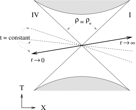
Figure 2: Schwarzschild black hole in Kruskal-Szeres coordinates. Spatial sections with $t=constant$ are space-like lines through the origin, going from region $IV$ to region $I$. $T$ and $X$ are the Kruskal-Szeres time-like and space-like directions respectively. The horizons are at $\rho=\rho_{+}$, which coincides with the minimal physical radius at the center $\rho=\rho_{\rm sd}$.

Notice that on each line, the coordinate $r$ from (73) runs from $r=0$ at the spatial infinity on the left-hand-side, to $r=\infty$ on the right-hand-side. The fixed point of the $\mathbb{Z}_{2}$-isometry (84) (now with $Q=0$) is positioned at the center of figure 2. The value of $r$ at this fixed point and the corresponding minimal physical radius is given by

$$r_{\rm sd}^{D-2}=\tfrac{1}{2}M\,,\hskip 56.9055pt\rho_{sd}^{D-2}=2M\,.$$ (85)

Note that this value of the physical radius corresponds to the horizon of the black hole, as can also be seen from figure 2. One can make the wormhole geometry visible by associating to every value of $r$ a $(D-1)-$sphere. Representing every $(D-1)-$sphere by a circle one obtains the wormhole picture of figure 1.

In the more general case (i.e. $Q\neq 0$), the $t=constant$ sections are still paths connecting two regions of the RN black hole. To see what these regions correspond to, it is helpful to draw a Carter-Penrose diagram, see figure 3. The wormhole geometry is qualitatively the same as in the Schwarzschild case. The position of the wormhole throat and the value of the minimal physical radius are given by

$$r_{\rm sd}^{D-2}=\tfrac{1}{4}(M^{2}-Q^{2})\,,\hskip 56.9055pt\rho_{sd}^{D-2}=M+\sqrt{M^{2}-Q^{2}}\,,$$ (86)

which again coincide with the horizon at $\rho=\rho_{+}$. The curvature singularity of the D-instanton solutions with $\mathsf{q}^{2}>0$ (39) at $r_{\rm c}=(\mathsf{q})^{1/D-2}$ are resolved in this uplifting and can now be understood as the usual coordinate singularity of the RN black hole outer event horizons (i.e. $\rho=\rho_{+}$, or $r^{2\,(D-2)}=(M^{2}-Q^{2})/4$).

Figure 3: Carter-Penrose diagram of RN black hole. The lines with $\rho=\rho_{+}$ are the horizons, which coincide with the minimal physical radius $\rho=\rho_{\text{sd}}$ in the center.

The extremal RN black hole (i.e. $M^{2}=Q^{2}$) is qualitatively different from the other cases. As one can see from (84), the $\mathbb{Z}_{2}$-isometry is gone. By taking the limit $M^{2}\rightarrow Q^{2}$ of a non-extremal black hole we see that the wormhole stretches to an infinitely long throat. The fixed point of the isometry goes to spatial infinity at $r=0$. This means that the extremal black hole has a ”one-sided” wormhole with a minimal physical radius $\rho_{0}^{D-2}=M$, and the full Kruskal-like extension is geodesically complete without need for a region $IV$. This situation is illustrated in figure 4.

Figure 4: The geometry of the extremal black hole as a ”one-sided” wormhole with minimal physical radius $\rho_{0}$.

4.4 Dilatonic Black Holes: $bc>2$

The instantons with $bc>2$ uplift to non-extremal dilatonic black holes, i.e. black hole solutions carried by a metric, a vector and a dilaton. In fact, the uplift is identical to a version of the black hole solution presented in [24]. To be more precise, the non-extremal dilatonic black hole solutions of [24] contain an extra parameter $\mu$. For generic values of this parameter the black hole solution is singular. One only obtains a regular solution if $\mu\sim\mathsf{q}$.

The uplift of the $bc>2$ instantons equals the $\mu\rightarrow 0$ limit of the non-extremal black hole solutions of [24]. Therefore, in contradistinction to the $bc=2$ case, we obtain a singular black hole solution. This singularity can only be avoided in two limiting cases. The singularity disappears both in the extremal limit (46) when $\mathsf{q}^{2}\rightarrow 0$ and in the Schwarzschild limit (45) when $q_{-}\rightarrow 0$, where the dilaton decouples.

5 Uplift to $p$-Branes

In section 4 we have discussed the uplift of the instantons of section 3 to higher-dimensional black hole solutions. It is therefore natural to consider the uplift to higher-dimensional $p$-branes. To this end it will be useful to first introduce the following nomenclature.

Non-extremal deformations of general $p$-branes have been considered in [26, 24]. These are solutions of the $(D+p+1)$-dimensional Lagrangian, defined over Minkowski space,

$$\mathcal{L}_{D+p+1}=\sqrt{-\hat{g}}\,[\hat{R}-\frac{1}{2}\,(\partial\hat{\phi})^{2}-\frac{1}{2\,(p+1)!}\,e^{a\hat{\phi}}\,\hat{G}_{(p+2)}^{2}]\,,$$ (87)

with the rank-$(p+2)$ field strength $\hat{G}_{(p+2)}=d\hat{C}_{(p+1)}$. For a $p$-brane in $D+p+1$ dimensions the metric (in Einstein frame) is of the form

$$ds^{2}=e^{2A}(-e^{2f}dt^{2}+dx_{p}{}^{2})+e^{2B}(e^{-2f}dr^{2}+r^{2}d\Omega_{D-1}{}^{2})\,,$$ (88)

where $A$, $B$ and $f$ are functions that depend on the radial coordinate $r$ only. It is convenient to introduce the quantity

$$X=(p+1)A+(D-3)B\,.$$ (89)

The extremal $p$-brane solutions with equal mass and charge, preserving half of the supersymmetry, are obtained by taking $X=f=0$.

Assuming that $D\geq 3$ there exist two types of non-extremal $p$-brane solutions in the literature. Following [24], we will call them type 1 and type 2 non-extremal $p$-branes:

• Type 1 non-extremal $p$-branes: $X=0$ and $f\neq 0$.

  These are the non-extremal black branes of [26, 27]. The deformation function $f$ is given by

  $$e^{2f}=1-\frac{k}{r^{D-2}}\,,$$ (90)

  where $k$ is the deformation parameter. In a different coordinate frame, with radial coordinates $\rho$, these branes can be expressed in terms of the two harmonic functions

  $$f_{\pm}(\rho)=1-\big{(}\frac{\rho_{\pm}}{\rho}\big{)}^{D-2}\,.$$ (91)

  Physical branes without a naked singularity have more mass than charge, which corresponds to $\rho_{+}>\rho_{-}$ or $k>0$. For this type of non-extremal deformation, the dilaton $\hat{\phi}$ is proportional to $A$ and $B$, which are linearly related since $X=0$.

• Type 2 non-extremal $p$-branes: $X\neq 0$ and $f=0$.

  These are the non-extremal black branes of [24]. The deformation function $X$ reads

  $$e^{X}=1-\frac{k}{r^{2(D-2)}}\,,$$ (92)

  where $k$ is the deformation parameter. The absence of naked singularities requires $k$ to be positive. In this case, the dilaton $\hat{\phi}$ is not proportional to $A$ or $B$, which are not linearly related.

  The non-extremal D-instanton solutions (39) fit exactly in this chain of non-extremal $p$-branes for $p=-1$. Although the type 2 non-extremal $p$-branes are defined in Minkowski space, we find that one can extend the formulae of [24] to $p=-1$ branes in Euclidean space, i.e. generalised D-instantons, by taking $f=0$ and $B\neq 0$.

Both types of non-extremal $p$-branes break supersymmetry. A special case is $p=0$, for which the regular type 1 and type 2 non-extremal $0$-branes are equivalent up to a coordinate transformation in $r$. From the form of the metric (88), which has different world-volume isometries for $f=0$ and $f\neq 0$, it is clear that this is not the case for $p>0$.

To relate the (multi-dilaton) instanton solutions of section 3 to the non-extremal $p$-branes, it is instructive to reduce the $p$-branes over their $(p+1)$-dimensional world-volume, including time. In complete analogy to the reduction over time of section 4.1, this will give rise to $p+1$ dilatons from the world-volume of the $p$-brane. However, these are not all unrelated: for one thing, the dilatons corresponding to the spatial world-volume will be proportional to each other, and can therefore be truncated to a single dilaton. We will denote the dilaton from the spatial metric components by $\varphi$, while the time-like component of the metric gives rise to $\tilde{\varphi}$. In general, the reduction of non-extremal $p$-branes will therefore give rise to a multi-instanton solution with three different dilatons, including the explicit dilaton $\phi$:

$$\hat{g}_{tt}\rightarrow\tilde{\varphi}\,,\qquad\hat{g}_{xx}\rightarrow\varphi\,,\qquad\hat{\phi}\rightarrow\phi\,.$$ (93)

For the two types of non-extremal deformations considered here, however, there is always a relation between the three dilatons, allowing a truncation to two dilatons. For the type 1 deformations the dilatons $\phi$ and $\varphi$ are related, as can be seen from the metric with $X=0$. Similarly, the type 2 deformations yield a relation between $\varphi$ and $\tilde{\varphi}$ since $f=0$. Therefore, these non-extremal $p$-branes reduce to multi-dilaton instanton solutions with two inequivalent dilatons. Conversely, two-dilaton instanton solutions can uplift to either types of non-extremal $p$-branes, by embedding these dilatons in different ways in the higher-dimensional metric and dilaton.

It is interesting to investigate when these two dilatons can be related or reduce to one, therefore corresponding to our explicit $SL(2,\mathbb{R})$ instanton solution (30) with only one dilaton. For the type 1 deformations, this is only possible for the special case with $p=0$ and $a=0$. For these values, the dilatons $\phi$ and $\varphi$ vanish, leaving one with only $\tilde{\varphi}$. The constraint on $a$ implies $bc=2$ which, as discussed in section 3, gives rise to the Reissner-Nordström black hole.

For the type 2 deformations there are more possibilities to eliminate the dilaton $\phi$. It can be achieved by requiring $a=0$, as we did for the uplift to black holes. For general $p$, this leads to the following constraint on $b$:

$$b=\sqrt{\frac{2(p+1)(D-2)}{D+p-1}}\,.$$ (94)

Note that this yields $bc=2$ for black holes with $p=0$. For these values of $b$, the instanton solution (30) can be uplifted to regular non-extremal non-dilatonic $p$-branes. For higher values of $b$, the instanton solution uplifts to singular non-extremal dilatonic $p$-branes. For these solutions to become regular, one must take either $\mathsf{q}^{2}\rightarrow 0$ or $q_{-}\rightarrow 0$, exactly like we found in the $bc>2$ discussion of section 4.3.

The uplift of the $SL(2,\mathbb{R})$ instanton solution (30) to $p$-branes is therefore very similar to the uplift to black holes. There is one value of $b$ (94) for which the instanton solution can be uplifted to a regular non-extremal non-dilatonic $p$-brane of type 2. For higher values of $b$ one can obtain singular non-extremal dilatonic $p$-branes of type 2, which only become regular on either of the limits $\mathsf{q}^{2}\rightarrow 0$ and $q_{-}\rightarrow 0$. By adding an extra dilaton to the instanton solution one can also connect to the regular type 1 and type 2 non-extremal dilatonic $p$-branes.

6 Instantons

In the previous section we focused on the bulk behavior of the three conjugacy classes of instanton-like solutions. In this section we will investigate which of these solutions can be interpreted as instantons. Instantons are defined to be solutions to the Euclidean equations of motion with finite, non-zero value of the action. They sometimes have a tunneling interpretation, but more generically, they contribute to certain correlation functions in the path integral, with terms that are exponentially suppressed by the instanton action. These correlation functions then induce new interactions in the effective action, and for the extremal, 1/2 BPS, D-instantons in type IIB in $D=10$, these effects are captured by certain $SL(2,\hbox{\mybb Z})$ modular functions that multiply higher derivative terms like $R^{4}$ and their superpartners [5]. Before we study correlation functions and effective interactions induced by non-extremal D-instantons, we must first discuss the properties and show the finiteness of the non-extremal instanton action. We will do this in such a way that the special case of extremal D-instantons can easily be recovered.

6.1 Instanton Action

The first thing we notice is that the action (24), evaluated on any solution of (27) vanishes. What is also bothersome about the Euclidean action (24) is that it is not bounded from below, not even in the scalar sector. Such actions cannot be used for a semiclassical approximation in the path integral, since fluctuations around the instanton will diverge. This problem can be solved by adding boundary terms that guarantee a positive definite action for the scalars, yielding at the same time a nonzero value for the instanton action. These boundary terms can be understood as coming from dualising the magnetic nine-form into the axion field $\chi$ [4, 5], subject to appropriate boundary conditions for the fields and their variations. This dual formulation has a manifestly positive definite action (apart from the usual problems with the Einstein-Hilbert term), in which it is easy to derive a Bogomol’nyi bound and therefore, the semiclassical approximation is justified. This procedure was also demonstrated in lower dimensions in [28].

The action for the dilaton and the “magnetic” $(D-1)$-form, dual to the axion $\chi$, can be written as [5]

$$\mathcal{S}_{E}=\int_{\mathcal{M}}\tfrac{1}{2}[(d\phi\wedge\ast d\phi+e^{-b\phi}F_{D-1}\wedge\ast F_{D-1})]\,,$$ (95)

supplemented by the constraint that $F_{D-1}$ is closed. Notice that in this formalism, the $SL(2,\mathbb{R})$ symmetry is not manifest.

We can dualise back to the dilaton-axion system by introducing a Lagrange multiplier $\chi$ that enforces the Bianchi-identity for $F_{D-1}$, i.e. ${\mathcal{L}}_{mult}=-\chi dF_{D-1}$. If we now algebraically eliminate $F_{D-1}$ from the action by treating it as a fundamental field (as opposed to treating it as a field strength) and using its equation of motion,

$$F_{D-1}=-e^{b\phi}\ast d\chi\ ,$$ (96)

we obtain the Euclidean action (24) in terms of the axion $\chi$ plus the boundary term mentioned above.

It is now easy to show that this action satisfies a Bogomol’nyi bound [5]. Using the fact that, in a Euclidean space, $\ast\ast A_{p}=(-)^{(D-1)p}A_{p}$, where $A_{p}$ is a $p$-form, we can rewrite the action as follows:

$$\mathcal{S}_{E}=\int_{\mathcal{M}}\tfrac{1}{2}[(d\phi\pm e^{-b\phi/2}\ast F_{D-1})\wedge\ast(d\phi\pm e^{-b\phi/2}\ast F_{D-1})\mp(-)^{D}\tfrac{4}{b}d(e^{-b\phi/2}F_{D-1})]\,,$$ (97)

where we have used the fact that $dF_{D-1}=0$. Since the first term is positive semi-definite $\mathcal{S}_{E}$ is bounded from below by a topological surface term given by the last term in (97). The bound is saturated when the Bogomol’nyi equation

$$\ast F_{D-1}=\mp e^{b\phi/2}d\phi\ ,$$ (98)

is satisfied. The $\mp$ distinguishes instantons from anti-instantons, and for simplicity, we will use the upper sign from now on. Using (96), one can write the Bogomol’nyi equation as

$$d\chi=-e^{-b\phi/2}d\phi\,,$$ (99)

and one can check explicitly that the instanton solutions with $\mathsf{q}^{2}=0$, given in (47), satisfy this bound. They are therefore rightfully called extremal. The instanton action can then easily be evaluated, and has only a contribution from the boundary at infinity,

$$\mathcal{S}^{\infty}_{{inst}}=\frac{4}{b^{2}}(D-2)\mathcal{V}ol(S^{D-1})\frac{|bcq_{-}|}{g_{s}^{b/2}}\ ,$$ (100)

while the contribution from $r=0$ vanishes.

For $D=10$ and $b=2$, this value of the instanton action precisely coincides with [4]. For other values of $b$, we notice the dependence of $g_{s}$ on $b$. In ten dimensions, the only possible value for $b$ compatible with maximal supersymmetry is $b=2$. One then finds that the instanton action depends linearly on the inverse string coupling constant. In lower dimensions this is not necessarily so, and more values for $b$ are possible, depending on whether $\chi$ comes from the RR sector or from the NS sector. This would imply different kinds of instanton effects, with instanton actions that depend on different powers of the string coupling constant. This indeed happens for instance in four dimensions, after compactifying type IIA strings on a Calabi-Yau threefold. There are D-instantons coming from wrapping (Euclidean) D2 branes around a supersymmetric three-cycle, and there are NS5-brane instantons coming from wrapping the NS5-brane around the entire Calabi-Yau. As explained in [29], such instanton effects are weighted with different powers of $g_{s}$ in the instanton action. This was also explicitly demonstrated in [28, 30, 31]. In our notation, they correspond to $b=1$ and $b=2$. Our results in (100) are consistent with these observations.

Notice also that the instanton action is proportional to $q_{-}$. For extremal instantons, this is precisely the mass of the corresponding black hole in one dimension higher, see (81). This is a generic characteristic of the instanton-soliton correspondence that we know from field theories. There, the Euclidean action in $D$ dimensions equals the Hamiltonian in $D+1$ dimensions, and the instanton action equals the soliton mass. It is interesting to see that this also happens for theories with gravity.

We now turn to the case of non-extremal instantons, and focus first on the case of $\mathsf{q}^{2}>0$. The solutions (39) for the dilaton and axion fields can be written as

$$d\phi=\frac{2}{b}\coth(H+C_{1})dH\ ,\qquad e^{-b\phi/2}F_{D-1}=\frac{2}{b}\frac{\ast dH}{\sinh(H+C_{1})}\,,$$ (101)

and do not satisfy the Bogomol’nyi equation (98). To evaluate the action on this non-extremal instanton solution, we plug in these expressions into the bulk action (95), and find

$$\mathcal{S}_{inst}=\frac{2}{b^{2}}\int\,d\Big{(}\{H-2\coth(H+C_{1})\}\ast dH\Big{)}\,,$$ (102)

which is again a total derivative term. Using Stokes theorem, we therefore only pick up contributions from the boundaries. Since the $\mathsf{q}^{2}>0$ instantons have a curvature singularity at $r=r_{c}$ (see section 3.1), one can take these boundaries at $r=\infty$ and at $r=r_{c}$. In terms of the variable $H$, this corresponds to $H=0$ and $H=\infty$ respectively. We remind again that we have taken $C_{1}$ to be positive, in order to avoid further singularities in the scalar sector when $H+C_{1}=0$.

Evaluating the Einstein-Hilbert term on the solution in (39) we find the following:

$$-\int_{\mathcal{M}}R =-\frac{2}{b^{2}}\,\int_{\mathcal{M}}d(H\ast dH)\,,$$ (103)

which precisely cancels the first term of the scalar action (102). Strictly speaking, both these terms diverge at the boundary $r=r_{c}$ as one can show, and need to be regularized. For the Einstein-Hilbert term, this needs to be done in combination with the Gibbons-Hawking term [33],

$$\mathcal{S}_{EH} =-\Big{(}\int_{\mathcal{M}}R+2\int_{\partial{\mathcal{M}}}(K-K_{0})\Big{)}\,,$$ (104)

where $\mathcal{M}$ is the $D$-dimensional Euclidean space and $\partial{\mathcal{M}}$ is the boundary. In the second term, $K$ is the trace of the extrinsic curvature of the boundary and $K_{0}$ the extrinsic curvature one would find for flat space, which is subtracted to normalise the value of the action. One can check that from the boundary at $r=\infty$, there is no contribution to (104). At $r=r_{c}$, the metric has a curvature singularity and the dilaton blows up; therefore the supergravity approximation breaks down. One would have to rely on higher order string theory corrections to regularize the contribution from $r_{c}$. Whatever the precise contribution is, we remark that the gravitational action (104) is an $SL(2,\mathbb{R})$ invariant, independent of the string coupling constant. It can therefore only be a function of $\mathsf{q}^{2}$.

If we assume that the regularization is such that there is still a cancellation with the first term in (102), we only have contributions coming from the second terms of both integrals (102) and (104). We first discuss the boundary at $r=\infty$. The contribution from (104) vanishes, while (102) yields a contribution

$$\mathcal{S}^{\infty}_{inst} =\frac{4}{b^{2}}\,(D-2)\mathcal{V}ol(S^{D-1})\,{b\,c}\,\Big{(}\mathsf{q}\,\coth C_{1}\Big{)}\,,$$

$$=\frac{4}{b^{2}}\,(D-2)\,\mathcal{V}ol(S^{D-1})\,b\,c\,\Big{(}\sqrt{\mathsf{q}^{2}+\frac{q_{-}^{2}}{g_{s}^{b}}}\Big{)}\ .$$ (105)

In the second line, we have used the relation between $C_{1}$ and the asymptotic value of the dilaton, $g_{s}^{b}=(q_{-}/\mathsf{q})^{2}\,\sinh^{2}C_{1}$.

For $\mathsf{q}^{2}=0$, (6.1) precisely yields back the result for the extremal instanton, see (100). There we made the relation between the instanton action and the black hole mass in one dimension higher. Also for the non-extremal instanton, such a relation seems to holds. Indeed, from the mass formula for the non-extremal black hole in terms of the instanton parameters, one has that $\mathsf{q}\,\coth C_{1}=\sqrt{\mathsf{q}^{2}+q_{-}^{2}}$, and the string coupling constant is set to unity. One therefore sees that the contribution to the instanton action from the boundary at infinity is proportional to the black hole mass in one dimension higher.

The boundary at $r=r_{c}$ receives contributions from both integrals (102) and (104), which add up to

$$\mathcal{S}^{r_{c}}_{inst} =\frac{4}{b^{2}}\,(D-2)\mathcal{V}ol(S^{D-1})\,{b\,c}\,\Big{(}\mathsf{q}\,(\frac{bc}{2}-1)\Big{)}\,.$$ (106)

Note that this contribution vanishes for the case $bc=2$, while it is positive for $bc>2$. However, as discussed above, it is not at all clear whether this contribution to the integrals (102) and (104) should be included in the instanton action, since it is calculated in a region of space where the supergravity approximation is no longer valid. It might well be that string corrections smooth out the singularity at $r=r_{c}$, leaving one with only the contribution (6.1) from $r=r_{\infty}$.

We now turn to the case of $\mathsf{q}^{2}<0$, or with $\mathsf{q}=i\mathsf{\tilde{q}}$, a positive $\mathsf{\tilde{q}}^{2}>0$. A similar calculation as for $\mathsf{q}^{2}>0$ shows that, for the solution (51), we have

$$d\phi=\frac{2}{b}\cot(\tilde{H}+\tilde{C_{1}})d\tilde{H}\ ,\qquad e^{-b\phi/2}F_{D-1}=\frac{2}{b}\frac{\ast d\tilde{H}}{\sin(\tilde{H}+\tilde{C_{1}})}\,,$$ (107)

where

$$\tilde{H}=bc\arctan(\frac{\tilde{q}}{r^{D-2}})\,,$$ (108)

is a harmonic function over the geometry given by the metric in (51). Plugging in these expressions into the bulk action (95), we find

$$\mathcal{S}_{inst}=-\frac{2}{b^{2}}\int\,d\Big{(}\{\tilde{H}+2\cot(\tilde{H}+{\tilde{C}_{1}})\}\ast d\tilde{H}\Big{)}\,.$$ (109)

Since this is a total derivative, we can use Stokes theorem again to reduce it to an integral over the boundaries. These boundaries are at $r=\infty$ and $r=0$, where we required that $bc<2$, as discussed in section 3.1. In contrast to the discussion of the $r=r_{c}$ boundary for $\mathsf{q}^{2}>0$, the instanton solution is perfectly regular everywhere, in particular at both boundaries. Therefore the contribution from the boundary at $r=0$ can also be trusted.

In addition to the above action, one also needs to include the gravitational contribution (104). Similar to the case of $\mathsf{q}^{2}>0$, the first term of (109) is cancelled by the contribution from the Ricci scalar. We anticipate the Gibbons-Hawking term not to contribute, since the two asymptotic geometries at $r=0$ and $r=\infty$ are equivalent due to the $\mathbb{Z}_{2}$-symmetry (84) and therefore their contributions should cancel.

Therefore the $\mathsf{q}^{2}<0$ instanton action has contributions only from the second term of (109) from both boundaries at $r=0$ and $r=\infty$:

$$\mathcal{S}_{inst}^{\infty} =\frac{4}{b^{2}}\,(D-2)\mathcal{V}ol(S^{D-1})\,{b\,c}\,\mathsf{\tilde{q}}\,\Big{(}\cot\tilde{C}_{1}\Big{)}\,,$$

$$\mathcal{S}_{inst}^{0} =\frac{4}{b^{2}}\,(D-2)\mathcal{V}ol(S^{D-1})\,{b\,c}\,\mathsf{\tilde{q}}\,\Big{(}-\cot(\tilde{C}_{1}+bc\frac{\pi}{2})\Big{)}\,.$$ (110)

Due to the fact that $\tilde{C}_{1}$ and $\tilde{C}_{1}+bc\pi/2$ are on the same branch of the cotangent (due to the restriction of regular scalars for $0<r<\infty$, which can only be achieved for $bc<2$, see section 3.1), the total instanton action is manifestly positive definite. In the neighborhood of $bc\approx 2$, the instanton action becomes very large, and the limit to the extremal point where $bc=2$, is discontinuous. This shows that this instanton is completely disconnected from the extremal D-instanton.

Using the asymptotic value of the dilaton in (51), we have $g_{s}^{b}=(q_{-}/\mathsf{\tilde{q}})^{2}\sin^{2}\tilde{C}_{1}$, and therefore $\mathsf{\tilde{q}}^{2}<q_{-}^{2}/g_{s}^{b}$. Assuming that $\cot\tilde{C}_{1}>0$, the contribution from infinity is positive and can be rewritten as

$$\mathcal{S}_{inst}^{\infty}=\frac{4}{b^{2}}\,(D-2)\,\mathcal{V}ol(S^{D-1})\,b\,c\,\sqrt{\frac{q_{-}^{2}}{g_{s}^{b}}-\mathsf{\tilde{q}}^{2}}\ ,$$ (111)

which is the analytic continuation of the result with $\mathsf{q}^{2}>0$.

6.2 Correlation Functions

Once the instanton solutions are established, one studies their effect in the path integral. As for D-instantons in ten-dimensional IIB, they contribute to certain correlation functions via the insertion of fermionic zero modes. For the D-instanton, which is 1/2 BPS, there are sixteen fermionic zero modes. These are solutions for the fluctuations that satisfy the linearised Dirac equation in the presence of the instanton. All of these zero modes can be generated by acting with the broken supersymmetries on the purely bosonic instanton solution. For the non-extremal instantons, no supersymmetries are preserved, so there are more fermionic zero modes. Let us focus for simplicity on ten-dimensional type IIB. Since all the supercharges are broken, one can generate 32 fermionic zero modes. The path integral measure contains an integration over these fermionic collective coordinates, and to have a non-vanishing result, one must therefore insert 32 dilatinos in the path integral. Based on this counting argument of fermionic zero modes, a 32-point correlator of dilatinos would be non-zero, and induce new terms in the effective action, containing 32 dilatinos. In the full effective action, such terms are related to higher curvature terms like e.g. certain contractions of $R^{8}$. An explicit instanton calculation should be done to determine the non-perturbative contribution to the function that multiplies $R^{8}$. As for the D-instanton, we expect that the contributions of the instantons with different $\mathsf{q}^{2}$-values build up a modular form with respect to $SL(2,\hbox{\mybb Z})$, possibly after integrating over $\mathsf{q}^{2}$.

These issues, though important, lie beyond the scope of this paper, and are left for further investigation.

7 Discussion

In this paper we investigated non-extremal instantons in string theory that are solutions of a gravity-dilaton-axion system with dilaton coupling parameter $b$. In particular, we constructed an $SL(2,\mathbb{R})$ family of radially symmetric instanton-like solutions in all conjugacy classes labelled by $\mathsf{q}^{2}$. Among these is the (anti-)D-instanton solution with $\mathsf{q}^{2}=0$. For special values of the dilaton coupling parameter this solution is half-supersymmetric. The instanton solutions in the other two conjugacy classes, with $\mathsf{q}^{2}>0$ and $\mathsf{q}^{2}<0$, are non-supersymmetric and can be viewed as the non-extremal version of the (anti-)D-instanton. This view is confirmed by the property that instantons in these two conjugacy classes, for $bc\geq 2$ with $c$ defined in (32), can be uplifted to non-extremal black holes.

We stressed the wormhole nature of the instanton solutions. We found that each conjugacy class leads to a wormhole geometry provided the corresponding instanton is given in a particular metric frame:

$$\mathsf{q}^{2}>0 \leftrightarrow {\rm dual\ frame\ metric\ (only~{}for~{}}bc=2{\rm~{}or~{}}q_{-}=0)$$

$$\mathsf{q}^{2}=0 \leftrightarrow {\rm string\ frame\ metric}$$ (112)

$$\mathsf{q}^{2}<0 \leftrightarrow {\rm Einstein\ frame\ metric}$$

For all these case the metric takes the form (52), with the specific values given in section 3.2.

Not all instanton solutions we constructed are regular and not all can be uplifted to black holes. The non-extremal instantons in the $\mathsf{q}^{2}>0$ conjugacy class all have a curvature singularity at $r=r_{\rm c}$, see (41). Only the $bc=2$ instanton can be uplifted to a regular non-extremal RN black hole with the singularity being resolved as a coordinate singularity at the outer event horizon of the RN black hole. The singularity remains for $bc>2$ and in that case can be resolved by adding an extra dilaton to the original system [21]. Two exceptions are the limits $\mathsf{q}^{2}\rightarrow 0$ or $q_{-}\rightarrow 0$, which correspond to the extremal and Schwarzschild black hole solutions, respectively. Finally, the instantons in the $\mathsf{q}^{2}<0$ conjugacy class are only regular for $bc<2$. These instantons can never be uplifted to black holes.

We have also considered the uplift of our instanton solutions to $p$-branes. It turns out that an instanton can only be uplifted over a $(p+1)$-torus to a $p$-brane provided the dilaton coupling satisfies (following from (94))

$$b\,c\geq\sqrt{\frac{4(p+1)(D-1)}{D+p-1}}\,.$$ (113)

For the case that saturates this bound, the instanton with $\mathsf{q}^{2}\geq 0$ uplifts to a regular non-dilatonic $p$-brane. For larger values of $b$, the instanton solution (30) with $\mathsf{q}^{2}>0$ uplifts to a singular limit of the dilatonic $p$-branes of [24]. These solutions only become regular in the limit $\mathsf{q}^{2}\rightarrow 0$ or $q_{-}\rightarrow 0$. A summary of the possible regular solutions is given in table 1. Alternatively, we have discussed the possibility of adding an extra dilaton to the instanton solution [21], which allows for the uplift to the regular dilatonic $p$-branes of both type 1 and type 2.

$bc$	Dimension	Regular solutions
$<2$	$D$	Instantons with $\mathsf{q}^{2}\leq 0$, see (51)
$=2$	$D+1$	RN black holes with $\mathsf{q}^{2}\geq 0$, see (73), or
		Schwarzschild black holes with $\mathsf{q}^{2}>0$, $q_{-}=0$
$>2$	$D+1$	Dilatonic black holes with $\mathsf{q}^{2}=0$ or
		Schwarzschild black holes with $\mathsf{q}^{2}>0$, $q_{-}=0$
$=$ in (113)	$D+p+1$	Non-dilatonic $p$-branes with $\mathsf{q}^{2}\geq 0$
$>$ in (113)	$D+p+1$	Dilatonic $p$-branes with $\mathsf{q}^{2}=0$ or
		$\mathsf{q}^{2}>0$, $q_{-}=0$

Table 1: The regular instanton, black hole and $p$-brane solutions that are obtained, depending on the dilaton coupling parameter $b$, the conjugacy class $\mathsf{q}^{2}$ and the charge $q_{-}$.

For the particular value $b=2$, corresponding to $\Delta=4$, there is another higher-dimensional origin. In this special case, the $D$-dimensional extremal instanton can be uplifted to a gravitational wave in $D+2$ dimensions [8]. Similarly, the other two conjugacy classes uplift to purely gravitational solutions in $D+2$ dimensions which we denominate “non-extremal waves”. The terminology is slightly misleading since the uplift only leads to a time-independent solution. Whether this solution can be extended to a time-dependent wave-like solution remains to be seen. It is also interesting to note the following curiosity. The source term for a pp-wave is a massless particle, i.e. a particle with a null-momentum vector: $p^{2}=0$. It is suggestive to associate the source terms for the other two conjugacy classes with massive particles ($p^{2}>0$) and tachyonic particles ($p^{2}<0$). We leave this for a future investigation.

In the second part of this paper we investigated the possibility whether the non-extremal instantons might contribute to certain correlation functions in string theory. For this application it is a prerequisite that there is a well-defined and finite instanton action. Mimicking the calculation of the standard D-instanton action we found that for $\mathsf{q}^{2}>0$ the contribution from infinity to the instanton action, for all values of $b$, is given by the elegant formula (6.1). This action reduces to the standard D-instanton action for $\mathsf{q}^{2}=0$. Having a finite action, the non-extremal instantons might contribute to certain correlation functions. In the case of type IIB string theory we conjectured that non-extremal instantons contribute to the $R^{8}$ terms in the string effective action in the same way that the extremal D-instantons contribute to the $R^{4}$ terms in the same action. Whether the fact that all supersymmetries are broken by the non-extremal instantons poses problems remains to be seen. An explicit instanton calculation should decide whether our conjecture is correct. This and related issues we leave for future investigation.

References

- [1] E. Bergshoeff, U. Gran and D. Roest, Type IIB seven-brane solutions from nine-dimensional domain walls, Class. Quant. Grav. 19 (2002) 4207–4226 hep-th/0203202.
- [2] E. Bergshoeff, M. de Roo, M. B. Green, G. Papadopoulos and P. K. Townsend, Duality of Type II 7-branes and 8-branes, Nucl. Phys. B470 (1996) 113–135 [hep-th/9601150].
- [3] E. Bergshoeff, M. Nielsen and D. Roest, The domain walls of gauged maximal supergravities and their M-theory origin, hep-th/0404100.
- [4] G. W. Gibbons, M. B. Green and M. J. Perry, Instantons and Seven-Branes in Type IIB Superstring Theory, Phys. Lett. B370 (1996) 37–44 hep-th/9511080.
- [5] M. B. Green and M. Gutperle, Effects of D-instantons, Nucl. Phys. B498 (1997) 195–227 hep-th/9701093.
- [6] S. B. Giddings and A. Strominger, String Wormholes, Phys. Lett. B230 (1989) 46.
- [7] D. H. Coule and K. i. Maeda, Class. Quant. Grav. 7 (1990) 955.
- [8] A. A. Tseytlin, Type IIB instanton as a wave in twelve dimensions, Phys. Rev. Lett. 78 (1997) 1864–1867 hep-th/9612164.
- [9] J. Y. Kim, H. W. Lee and Y. S. Myung, D-instanton and D-wormhole, Phys. Lett. B400 (1997) 32–36 hep-th/9612249.
- [10] M. B. Einhorn and L. A. Pando Zayas, On seven-brane and instanton solutions of type IIB, Nucl. Phys. B582 (2000) 216–230 hep-th/0003072.
- [11] M. B. Einhorn, Instantons of type IIB supergravity in ten dimensions, Phys. Rev. D66 (2002) 105026 hep-th/0201244.
- [12] M. Gutperle and W. Sabra, Instantons and wormholes in Minkowski and (A)dS spaces, Nucl. Phys. B647 (2002) 344–356 hep-th/0206153.
- [13] J. Y. Kim, Y. b. Kim and J. E. Hetrick, arXiv:hep-th/0301191.
- [14] V. V. Khoze, From branes to branes, hep-th/0311065.
- [15] E. Bergshoeff and K. Behrndt, D-instantons and asymptotic geometries, Class. Quant. Grav. 15 (1998) 1801–1813 hep-th/9803090.
- [16] E. Bergshoeff and A. Van Proeyen, The many faces of , Class. Quant. Grav. 17 (2000) 3277–3304 hep-th/0003261.
- [17] M. B. Einhorn, Instantons and SL(2,R) symmetry in type IIB supergravity, hep-th/0212322.
- [18] P. Meessen and T. Ortín, An Sl(2,Z) multiplet of nine-dimensional type II supergravity theories, Nucl. Phys. B541 (1999) 195–245 hep-th/9806120.
- [19] H. J. Boonstra, K. Skenderis and P. K. Townsend, The domain wall/QFT correspondence, JHEP 01 (1999) 003 hep-th/9807137.
- [20] K. Behrndt, E. Bergshoeff, R. Halbersma and J. P. van der Schaar, On domain-wall/QFT dualities in various dimensions, Class. Quant. Grav. 16 (1999) 3517–3552 hep-th/9907006.
- [21] E. Cremmer, I. V. Lavrinenko, H. Lu, C. N. Pope, K. S. Stelle and T. A. Tran, Euclidean-signature supergravities, dualities and instantons, Nucl. Phys. B534 (1998) 40–82 hep-th/9803259.
- [22] H. Lu, C. N. Pope, E. Sezgin and K. S. Stelle, Stainless super p-branes, Nucl. Phys. B456 (1995) 669–698 hep-th/9508042.
- [23] P. K. Townsend, Black holes, gr-qc/9707012.
- [24] H. Lu, C. N. Pope and K. W. Xu, Liouville and Toda Solutions of M-theory, Mod. Phys. Lett. A11 (1996) 1785–1796 hep-th/9604058.
- [25] G. W. Gibbons and K.-i. Maeda, Black holes and membranes in higher dimensional theories with dilaton fields, Nucl. Phys. B298 (1988) 741.
- [26] G. T. Horowitz and A. Strominger, Black strings and P-branes, Nucl. Phys. B360 (1991) 197–209.
- [27] M. J. Duff and J. X. Lu, Black and super p-branes in diverse dimensions, Nucl. Phys. B416 (1994) 301–334 hep-th/9306052.
- [28] U. Theis and S. Vandoren, Instantons in the double-tensor multiplet, JHEP 09 (2002) 059 hep-th/0208145.
- [29] K. Becker, M. Becker and A. Strominger, Five-branes, membranes and nonperturbative string theory, Nucl. Phys. B456 (1995) 130–152 hep-th/9507158.
- [30] M. Davidse, M. de Vroome, U. Theis and S. Vandoren, Instanton solutions for the universal hypermultiplet, Fortsch. Phys. 52 (2004) 696–701 hep-th/0309220.
- [31] M. Davidse, U. Theis and S. Vandoren, Fivebrane instanton corrections to the universal hypermultiplet, hep-th/0404147.
- [32] E. Bergoeshoeff, A. Collinucci, U. Gran, D. Roest and S. Vandoren, Non-extremal instantons and wormholes in string theory, proceedings of the RTN2004 workshop, 5-10 September, Kolymbari, Crete, Greece, hep-th/0412183.
- [33] G. W. Gibbons and S. W. Hawking, Action integrals and partition functions in quantum gravity, Phys. Rev. D15 (1977) 2752–2756.