On The Problem of Particle Production in $c=1$ Matrix Model

Partha Mukhopadhyay

Department of Physics and Astronomy

University of Kentucky, Lexington, KY-40506, U.S.A.

E-mail: partha@pa.uky.edu

Abstract

We reconsider and analyze in detail the problem of particle production in the time dependent background of $c=1$ matrix model where the Fermi sea drains away at late time. In addition to the moving mirror method, which has already been discussed in hep-th/0403169 and hep-th/0403275, we describe yet another method of computing the Bogolubov coefficients which gives the same result. We emphasize that these Bogolubov coefficients are approximately correct for small value of the deformation parameter.

We also study the time evolution of the collective field theory stress-tensor with a special point-splitting regularization. Our computations go beyond the approximation of the previous treatments and are valid at large coordinate distances from the boundary at a finite time and up-to a finite coordinate distance from the boundary at late time. In this region of validity our regularization produces a certain singular term that is precisely canceled by the collective field theory counter term in the present background. The energy and momentum densities fall off exponentially at large distance from the boundary to the values corresponding to the static background. This clearly shows that the radiated energy reaches the asymptotic region signaling the space-time decay.

1 Introduction and Summary

Two dimensional bosonic and type 0B string theories have non-perturbative dual description in terms of the $c=1$ matrix model. Although the CFT description is quite complicated [8, 9, 10, 11] the matrix model description is simple. In the singlet sector this reduces to the quantum mechanics of an infinite (but fixed) number of non-relativistic free fermions in an inverted harmonic oscillator potential. Recently there has been a crucial progress in this subject through the understanding of the unstable D0 brane [12] and its decay on the matrix model side [13, 14, 15, 16]. Here also the matrix model description [16] of this decay turns out to be quite simpler than the BCFT description [19]. It is this simplicity of the matrix model description and the fact that it provides us with a non-perturbative definition of the theory enable us to probe various issues that would have been difficult to address otherwise (see, for example, [17]). Therefore it is important to study various other backgrounds, in particular the time dependent backgrounds [20, 21, 22, 23, 24, 25, 26, 27], in the matrix model itself to help understanding the corresponding world-sheet theories. This might provide us with clues on how to deal with time dependent backgrounds in string theory in general.

Recently in [23], some interesting fermionic configurations in the matrix model were viewed as two dimensional cosmological solutions. A particular class of time dependent solutions with two parameters were discussed where the envelop of the Fermi sea, having the same structure as the static one, has an overall motion on the single particle phase space. The motion is such that the Fermi sea floods in and subsequently drains away thus describing creation and the subsequent annihilation of the universe. They have been interpreted to be arising from the closed string tachyon condensation [23, 24, 26]. The corresponding world-sheet deformation was also suggested. Switching off one of the two parameters one reaches two different classes of one parameter solutions where the Fermi sea merges with the static one in either the past or the future asymptote. In this case the deformation parameter does not really parameterize inequivalent solutions as the change in this parameter can be absorbed by time translation. The solution, hereafter called the “draining Fermi sea”, in which the Fermi sea starts from a configuration arbitrarily close to the static one at early time and drains away at late time has been further studied in [24, 25] where the problem of cosmological particle production has been addressed. In particular in [25] the Bogolubov coefficients for the particle production have been computed explicitly. An approximate analysis of the energy-momentum tensor was also performed and it was argued that the contribution to the energy coming from particle production and the time evolution of the initial vacuum energy cancel so that the net energy remains the same.

In this paper we study the same questions in more detail. In the static background the theory is free far away from the tachyon wall. In the draining background the tachyon wall moves in such a way that an observer initially sitting in the free region gradually enters the strongly coupled region where the notion of the massless particle is lost and the theory becomes more complicated. Nevertheless there is a time span during which the observer stays in the free region and can observe particle production. We attempt to quantify this observation during this particular span of time. Although the deformation parameter $\lambda$ corresponding to this background can be changed by time translation we fix the origin of time and treat $\lambda$ as an actual parameter. In this time-frame the condition for the observer not to enter the strongly coupled region during the whole process of observing particle production turns out to be $\ln 1/2\lambda>>0$. We shall see that this condition will be essential for computing approximate Bogolubov coefficients for the particle production.

In the first analysis of the system we study the computation of the Bogolubov coefficients in two different methods namely, the “scattering method” and the “moving mirror method”. The first method is directly related to the wall-scattering in the static background and uses crucially the Seiberg bound [35, 36] on the spectrum of primary operators in the CFT [8, 9, 10, 11]. The space-time version [3] of this bound is that the in-states of this particular scattering problem contains only the right-moving excitations which move toward the wall. Similarly the out-states contain only the left moving excitations. Application of the same bound in the time dependent case implies that the in and out-vacua support only the right and left-moving excitations respectively. In the static case the result of the classical wall-scattering is given by a “scattering equation” [33] where a right-moving oscillator is expressed in terms of the left-moving oscillators in the form of a power series, the leading term being linear and of order $g_{s}^{0}$. Therefore computing the scattering equation up-to the leading order in the time dependent case should give us the Bogolubov coefficients. Although this scattering equation is classical, non-trivial Bogolubov coefficients, which indicate quantum phenomenon like particle production, can be obtained with the following additional input. The motion of the moving Fermi sea on the phase-space can be undone by a time dependent canonical transformation which can be lifted to a coordinate transformation on the collective field [23, 25]. Implementing this coordinate transformation on the scattering equation in the static background gives non-trivial mixing between the positive and negative frequency modes. It turns out that this analysis gives approximate Bogolubov coefficients for small $\lambda$ such that $\ln 1/2\lambda>>0$.

In the moving mirror method, which has already been discussed in [24, 25], we set up the whole problem in the framework of the Das-Jevicki collective filed theory [39]. We work at the linearized level of the equation of motion which corresponds to taking a formal $g_{s}\to 0$ limit. In this approximation the problem of particle production in the moving Fermi sea backgrounds reduces to that of a moving mirror problem with reflecting boundary condition. This subject has been studied quite extensively in flat-space [42, 43, 44, 45]. In our case, it turns out that the metric is time dependent and therefore, as expected, introduces problems in defining the natural modes that should correspond to particles. In flat space examples of moving mirror one uses a certain argument of geometrical optics to construct the natural in and out-modes. We generalize this construction to the present case at hand.

The class of moving Fermi sea backgrounds are such that asymptotically the mirror approaches the velocity of light. In the draining Fermi sea background, which we concentrate on, this happens at the future asymptote where the mirror moves toward the observer. In a standard moving mirror example [42] one assumes that at far future the mirror approaches a constant velocity less than that of light so that the motion can be undone by a Lorentz transformation. In case of a mirror approaching the velocity of light toward the observer the whole portion of the future null asymptote is not available for defining the modes. In fact the natural out-modes that are constructed following the method of geometrical optics form an over-complete set in that region which destroys the orthonormality of these modes. It turns out that for the particular mirror-trajectory involved in our example the upper bound on the future null infinity is given by $\ln 1/2\lambda$. Therefore taking $\ln 1/2\lambda>>0$ we make these out-modes approximately orthonormal. The Bogolubov coefficients computed using these out-modes are therefore approximately correct for small $\lambda$. As expected from the fact that $\lambda$ acts as a deformation parameter, both the above methods give trivial Bogolubov coefficients in the limit $\lambda\to 0$. Therefore our results are approximately correct for small but nonzero $\lambda$.

Next we turn to the analysis of the stress-tensor and go beyond the approximation made in [25] (see the last part of the discussion in sec.6 for more details). Incorporating the effect of the non-flat metric we explicitly compute the vacuum expectation value of the stress-tensor by expanding field in terms of the in-modes constructed in the moving mirror discussion. Doing the computation in a point-splitting regularization method we encounter the usual vacuum ambiguity. Das-Jevicki collective field theory [39] automatically comes with a particular counter term which fixes this ambiguity (see [25] for a recent discussion). This counter term was first obtained in [38] using the collective field method [37] which is formally background independent. It was also showed by Gross and Klebanov in their “fermionic string field theory” formulation [40] that this counter term is equivalent to the normal ordering directly obtained from the fermionic theory. Considering the static case first, we show that in the computation using the mode expansion the known result is reproduced by a special type of point-splitting regularization method. We generalize this method to the time dependent case and obtain results for both the singular and finite parts of the stress-tensor components. We justify this regularization by showing that the counter term in the Hamiltonian required to cancel the singular part precisely agrees with the collective field theory counter term evaluated at the present background. We should mention at this point that our computations are actually done in a metric which is simpler than the actual one. This gives rise to a particular region of validity only where we achieve the above agreement. The region of validity of our analysis is (1) everywhere at early time, (2) large coordinate distances from the boundary at a finite time and (3) up-to a finite coordinate distance from the boundary at late time. The finite part of the energy density approaches the value corresponding to the static background at early time but evolves into something else at late time giving rise to a nonzero radiated energy. We show that the energy and momentum densities fall off exponentially to the values corresponding to the static background at large distance from the boundary.

The rest of the paper is organized as follows. We review some of the basic relevant points of both the world-sheet theory and the matrix model in sec.2. The time dependent backgrounds discussed in [23] are reviewed in sec.3. The two methods of computing the Bogolubov coefficients are given in subsections 4.1 and 4.2. Sec.5 contains the stress-tensor analysis. Finally, we conclude in sec.6 where we summarize the basic accomplishments of this paper and compare our stress-tensor analysis with those preexisted [24, 25, 26] in the literature. The appendices contain some of the technical details. We discuss the relation between the Bogolubov and the stress-tensor analysis in appendix D.

2 Review of Basic Facts

Here we touch upon the basic features of the world-sheet and the matrix model descriptions relevant for our discussion and spell out the dictionary of the duality.

2.1 The World-Sheet Theory

In addition to the usual time-like scalar $X^{0}$, the matter part of the world-sheet theory contains only one space-like scalar $X^{1}$ whose action is given by a particular limit of the Liouville action [8, 9, 10, 11],

$$S_{L} = \frac{1}{2\pi}\int d^{2}z\left(\partial X^{1}\bar{\partial}X_{1}+2\pi\mu_{0}e^{2bX^{1}}\right)~{},$$ (2.1)

with a background charge $Q=b+1/b$ and central charge $c_{L}=1+6Q^{2}$. The space of normalizable states is given by the collection of the conformal families corresponding to a one parameter family of primaries given by,

$$V_{Q+iw}=e^{(Q+iw)X^{1}}~{},\quad\quad 0\leq w<\infty~{},$$ (2.2)

with conformal dimension $(Q^{2}+w^{2})/4$. Notice that $w$ is restricted to be positive, the so-called Seiberg bound [35, 36]. In fact the operators with negative values of $w$ are related to the above ones by the following reflection equation,

$$V_{Q+iw} = R(w)V_{Q-iw}~{},$$ (2.3)

$$R(w) = -\mu^{-iw/b}\frac{\Gamma(1+iw/b)\Gamma(1+iwb)}{\Gamma(1-iw/b)\Gamma(1-iwb)}~{},$$ (2.4)

$$\mu = \pi\mu_{0}\gamma(b^{2})~{},\quad\gamma(x)=\frac{\Gamma(x)}{\Gamma(1-x)}~{}.$$ (2.5)

The world-sheet theory $S_{X^{1}}$ relevant for string theory is obtained (at $\alpha^{\prime}=1$) by taking the following limit,

$$b\to 1~{},\quad\mu_{0}\to\infty~{},\quad\mu~{}\hbox{fixed}~{}.$$ (2.6)

It turns out that it is only the combination $\mu/g_{s}$ which appears as a parameter in all the amplitudes so that there is only one parameter of the string theory which we take to be $g_{s}$. BRST analysis of the world-sheet theory shows that there is only one space-time field-theoretic degree of freedom, namely the “massless tachyon” given by the vertex operators,

$$V_{w}^{\pm}=c\bar{c}e^{-iwX^{0}}V_{2\pm iw}=c\bar{c}e^{-iw(X^{0}\mp X^{1})}e^{2X^{1}}~{},\quad w>0~{}.$$ (2.7)

The space-time interpretation of the reflection equation (2.5) or the Seiberg bound $w>0$ in the above equation goes in the following way (see, for example [3]). The effective coupling $g_{eff}=g_{s}e^{2x^{1}}$ falls off to zero at large negative $x^{1}$ where we have a free massless particle [36]. Because of the Liouville interaction-wall in (2.1) any right-moving pulse created in the free region necessarily results into left-moving pulses due to the scattering from the wall. Therefore in this scattering problem the in and out-states always contain only the right ($V_{w}^{+}$) and left-movers ($V_{w}^{-}$) respectively. In the second quantized theory these states are created by harmonic oscillators $\bar{a}^{in\dagger}_{w}$ and $\bar{a}^{out\dagger}_{w}$ respectively. We take the following normalization.

$$[\bar{a}^{in}_{w},\bar{a}^{in\dagger}_{w^{\prime}}]=[\bar{a}^{out}_{w},\bar{a}^{out\dagger}_{w^{\prime}}]=\delta(w-w^{\prime})~{}.$$ (2.8)

Then one concludes from (2.5) with the proper limit (2.6) that to the leading order in $g_{s}$, $\bar{a}^{in}_{w}$ is proportional to $\bar{a}^{out}_{w}$ where the proportionality constant is simply a $w$ dependent phase.

2.2 The Matrix Model

In the singlet sector, the c=1 matrix model reduces to the quantum mechanics of an infinite (but fixed) number of non-relativistic free fermions in an inverted harmonic oscillator potential given by $-x^{2}/2$. $g_{s}$ plays the role of the Planck’s constant $\hbar$ of the fermion theory. The string theory Hamiltonian is given by the second quantized Hamiltonian of these fermions with an additional factor of $1/g_{s}$ [33]. The closed string background discussed in the previous section corresponds to a particular classical state where all the single particle phase-space trajectories below energy $-1/2$ are filled by fermions. For the bosonic case, which is under consideration in this paper, only those trajectories which are on the left side of the potential are filled so that the envelop of the (static) Fermi sea is given by,

$$(x+p)(x-p) = 1~{},\quad x\leq-1~{}.$$ (2.9)

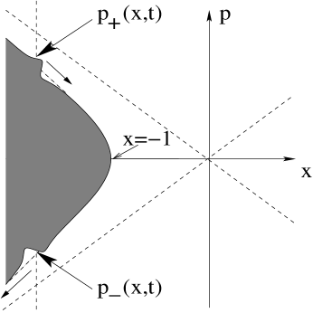
Figure 1: The “static Fermi sea” background which is dual to the closed string background with linear dilaton and static tachyon wall. The fluctuation of the upper and lower edges (which propagate along the direction of the arrows) give rise to the massless tachyon field.

Let $p_{\pm}(x,t)$ be the values of $p$ at the fluctuating upper and lower edges (fig.1). Then the fluctuations $\eta_{\pm}(x,t)$ are defined as,

$$p_{\pm}(x,t)=p_{0\pm}(x)+\eta_{\pm}(x,t)~{},$$ (2.10)

where the background is given by,

$$p_{0\pm}(x)=\pm P_{0}(x)~{},\quad P_{0}(x)=\sqrt{x^{2}-1}~{},\quad x\leq-1~{}.$$ (2.11)

Using Polchinski’s bosonization in [33] we define the fluctuations of the scalar field and the conjugate momentum, denoted by $\bar{\phi}(x,t)$ and $\pi_{\bar{\phi}}(x,t)$ respectively,

$$\eta_{\pm}(x,t)=\sqrt{\pi}g_{s}\left[-\pi_{\bar{\phi}}(x,t)\pm\partial_{x}\bar{\phi}(x,t)\right]~{}.$$ (2.12)

$x=-1$ acts as a boundary where $\bar{\phi}$ satisfies a Dirichlet boundary condition: $\bar{\phi}(x=-1,t)=0$. The static Fermi sea background (2.11) is given, in terms of the collective variables, as,

$$\partial_{x}\bar{\phi}^{(S)}_{0}(x,t)={P_{0}(x)\over\sqrt{\pi}g_{s}}~{},\quad\pi_{\bar{\phi}^{(S)}_{0}}(x,t)=0~{}.$$ (2.13)

Defining the new coordinate $q$,

$$x=-\cosh q~{},\quad-\infty<q\leq 0~{},$$ (2.14)

so that $P_{0}=|\sinh q|$, $P_{0}\partial_{x}=\partial_{q}$, the linearized equation of motion takes the form,

$$(\partial_{t}^{2}-\partial_{q}^{2})\phi=0~{},$$ (2.15)

where $\phi(q,t)=\bar{\phi}(x,t)$. It turns out that at $q<<0$ the non-linear parts of the equation of motion reduce to an infinite series of interaction terms with $g_{eff}=g_{s}e^{2\tilde{q}}~{}(\tilde{q}=q+\ln 2)$ as an effective coupling. In this region the fluctuation $\phi(q,t)$ can be mode expanded as,

$$\phi = \phi_{in}(u)+\phi_{out}(v)~{},$$ (2.16)

$$\phi_{in}(u) = \int_{0}^{\infty}{dw\over\sqrt{4\pi w}}\left[a^{in}_{w}e^{-iwu}+h.c.\right]~{},$$ (2.17)

$$\phi_{out}(v) = \int_{0}^{\infty}{dw\over\sqrt{4\pi w}}\left[a^{out}_{w}e^{-iwv}+h.c.\right]~{},$$ (2.18)

where $u=t-q$ and $v=t+q$ are the usual null coordinates. The oscillators $a^{in}_{w}$ and $a^{out}_{w}$ have the same normalization as in (2.8). The scalar field $S(q,t)$ introduced in [33], is related to $\phi(q,t)$ at $q<<0$ in the following way: $S(\tilde{q},t)=\phi(q,t)$. Therefore the oscillators, say $\tilde{a}^{in}_{w}$ and $\tilde{a}^{out}_{w}$, of $S(q,t)$ are related to that of $\phi(q,t)$ as follows: $a^{in}_{w}=e^{iw\ln 2}\tilde{a}^{in}_{w}$, $\quad a^{out}_{w}=e^{-iw\ln 2}\tilde{a}^{out}_{w}$. Using the result obtained in [33], we get the following scattering equation,

$$a^{in}_{w}=e^{iw\ln 4}a^{out}_{w}+O(g_{s})~{}.$$ (2.19)

The oscillators of the scalar field directly coming from string theory are related to the above oscillators through the leg-pole factors [28, 41, 32] with the additional phase factor described above.

$$\bar{a}^{in}_{w}={\Gamma(iw)\over\Gamma(-iw)}e^{-iw\ln 2}a^{in}_{w}~{},\quad\bar{a}^{out}_{w}={\Gamma(-iw)\over\Gamma(iw)}e^{iw\ln 2}a^{out}_{w}~{}.$$ (2.20)

The above derivation of the collective field theory is classical. Therefore in the process of quantization one encounters the usual vacuum ambiguity which has to be fixed by a normal ordering prescription. In the string field theory of Gross and Klebanov [40], which was shown to be equivalent to that of Das and Jevicki [39], this automatically came from the normal ordering of the fermionic theory. In Das-Jevicki field theory this is incorporated by a particular counter term first computed in [38] using the collective field method [37]. In our notation this counter term is given by,

$$\Delta H={g_{s}\over 2\sqrt{\pi}}\int_{-\infty}^{-1}dx~{}\partial_{x}\bar{\phi}(x,t)\partial_{x}\partial_{x^{\prime}}\ln|x-x^{\prime}|_{x=x^{\prime}}~{}.$$ (2.21)

According to the collective field derivation [38] this counter term is background independent.

3 The Moving Fermi Sea Backgrounds

We shall now consider a particular class of two-parameter time-dependent closed string backgrounds discussed in [23]. On the matrix model side this is described by a moving Fermi sea whose envelop is given by,

$$(x+p+2\lambda_{+}e^{t})(x-p+2\lambda_{-}e^{-t}) = 1~{},\quad x\leq x_{m}(t)~{},~{}~{}x_{m}(t)=-(1+\lambda_{+}e^{t}+\lambda_{-}e^{-t})~{}.$$ (3.22)

The envelop of the Fermi surface is an hyperbola which moves like a rigid body following the hyperbolic trajectory of its centre: $x_{0}(t)=-(\lambda_{+}e^{t}+\lambda_{-}e^{-t})~{},~{}~{}p_{0}(t)=-(\lambda_{+}e^{t}-\lambda_{-}e^{-t})$. Just like as described in the previous section the fluctuation of this Fermi surface also gives rise to a ($1+1$)-dimensional scalar field $\phi(t,q)$ which, at any given instant of time, behaves like a free massless field at a sufficiently large negative $q$. On the phase-space this configuration can be transformed into the static sea by the following time-dependent canonical transformation,

$$X=x+\lambda_{+}e^{t}+\lambda_{-}e^{-t}~{},\quad P=p+\lambda_{+}e^{t}-\lambda_{-}e^{-t}~{},\quad-\infty<X\leq-1~{}.$$ (3.24)

Following the usual method as described in subsection 2.2 a $(1+1)$ dimensional scalar field theory can be constructed from the static configuration in the $XP$-plane. We shall, in this case, use upper case symbols for various objects discussed in the previous section. We relate the space-time of this field theory with the original (matrix model) space-time $(x,t)$ by the following coordinate transformation,

$$X=x+\lambda_{+}e^{t}+\lambda_{-}e^{-t}~{},\quad T=t~{}.$$ (3.25)

Following (2.14) we define new coordinates $Q$ and $q$ as,

$$X = -\cosh Q~{},\quad-\infty<Q\leq 0~{},$$ (3.26)

$$x = -\cosh q~{},\quad-\infty<q\leq q_{m}(t)~{},$$ (3.27)

$$q_{m}(t) = -\cosh^{-1}(1+\lambda_{+}e^{t}+\lambda_{-}e^{-t})~{},$$ (3.28)

such that,

$$\cosh Q=\cosh q-(\lambda_{+}e^{t}+\lambda_{-}e^{-t})~{}.$$ (3.29)

At large negative $Q$ this reduces to $Q=q-\ln(1-2\lambda_{+}e^{v}-2\lambda_{-}e^{-u})$ such that,

$$U=u+\ln(1-2\lambda_{+}e^{v}-2\lambda_{-}e^{-u})~{},\quad V=v-\ln(1-2\lambda_{+}e^{v}-2\lambda_{-}e^{-u})~{},$$ (3.30)

where as usual we have defined: $U=T-Q,~{}V=T+Q$. The scattering equation for the oscillators $A^{in}_{w}$ and $A^{out}_{w}$ of the scalar field $\Phi(Q,t)$ will then be given by the same equation as (2.19),

$$A^{in}_{w}=e^{iw\ln 4}A^{out}_{w}+O(g_{s})~{}.$$ (3.31)

4 Bogolubov Analysis

For our explicit analysis we shall consider the draining Fermi sea background in which case we have in mind all the equations of the previous section with $\lambda_{+}=\lambda,~{}\lambda_{-}=0$. On the matrix model side the wall scattering of the massless particles can be computed [33] very easily by exploiting the fact that the classical trajectories of the fermions on the phase-space are exactly known.

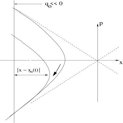
Figure 2: In the draining Fermi sea background the observer initially sitting far away from the wall at $q_{o}<<0$ gradually enters the strongly coupled region.

Given an incoming pulse created on the upper edge of the Fermi sea at $q<<0$ one can compute the deformed outgoing pulse that re-emerges, after some time on the lower edge without worrying about the complicated self interactions that the pulse goes through. In the draining Fermi sea background, as time evolves the wall moves toward left (fig.2) so that the observer gradually enters the strongly coupled region. We want to study the system over a time span during which the observer remains in the free region. If a pulse is sent in by the observer at a time $t_{-}(<<0)$ which is taken to be of the same order of the observer’s position $q_{o}(<<0)$ then the time at which the pulse is received back is given by,

$$t_{+}=-q_{o}-\ln(1+2\lambda)~{}.$$ (4.32)

The boundary of the space $q_{m}(t)$, which is zero at $t=t_{-}$, is given, at $t=t_{+}$, by,

$$q_{m}(t_{+})=-\ln 2\lambda-t_{+}+O(1/\lambda e^{t_{+}})=q_{o}-\ln\left({2\lambda\over 1+2\lambda}\right)~{},$$ (4.33)

where we have taken $e^{q_{o}}<<{\lambda\over 1+2\lambda}$. To keep $q_{o}$ in the free region at $t=t_{+}$ we should have $q_{o}-q_{m}(t_{+})<<0$. These two conditions can be written as,

$$-q_{o}>>\ln 1/2\lambda>>0~{}.$$ (4.34)

We shall see that to compute the Bogolubov coefficients we need to work with sufficiently small $\lambda$ so as to be consistent with the above equation. Then given a small value of $\lambda$ it also gives an estimation for the position of our observer.

4.1 Bogolubov Coefficients - Scattering Method

Let us now proceed to compute the Bogolubov coefficients. These are the coefficients of the linear expansion of the out-oscillators in terms of the in-oscillators where a mixing between the positive and negative frequency modes occur. One may, therefore, wonder if the leading order scattering equation obtained by the method of [33] can give these coefficients. In spite of the fact that the analysis of [33] gives only the tree-level results, with an additional input of coordinate transformation it is indeed able to capture particle production which is a quantum effect. At late time, the natural oscillators in the draining Fermi sea background are $a^{out}_{w}$, whereas at early time these are given by,

$$a^{in}_{w}=A^{in}_{w}=e^{iw\ln 4}A^{out}_{w}+O(g_{s})~{}$$ (4.35)

where the first equality is due to the fact that at early time the draining background merges with the static one and in the second step we have used the scattering equation (3.31) in the static background. The Bogolubov coefficients, therefore, effectively relate $a^{out}$ and $A^{out}$ oscillators.

$$a^{out}_{w}=\int_{0}^{\infty}dw^{\prime}\left[\alpha(w,w^{\prime})A^{out}_{w^{\prime}}+\beta(w,w^{\prime})A^{out\dagger}_{w^{\prime}}\right].$$ (4.36)

These coefficients can then in turn be computed by using the transformation,

$$\partial_{v}\phi=\partial_{v}U\partial_{U}\Phi+\partial_{v}V\partial_{V}\Phi~{},$$ (4.37)

and setting $\partial_{U}\Phi=0$ at late time which is the main use of Seiberg bound in the present analysis. For small $\lambda$ we get the following results (see appendix A for details),

$$\alpha(w,w^{\prime}) = \sqrt{w\over w^{\prime}}\int_{-\infty}^{\ln 1/2\lambda}{dx\over 2\pi}e^{iwx-iw^{\prime}f_{\lambda}(x)}~{},$$ (4.38)

$$\beta(w,w^{\prime}) = \sqrt{w\over w^{\prime}}\int_{-\infty}^{\ln 1/2\lambda}{dx\over 2\pi}e^{iwx+iw^{\prime}f_{\lambda}(x)}~{},$$ (4.39)

where the function $f_{\lambda}(x)$ is given by,

$$f_{\lambda}(x)=x-\ln(1-2\lambda e^{x})~{},\quad-\infty<x<\ln 1/2\lambda~{}.$$ (4.40)

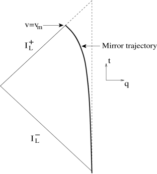
Figure 3: The asymptotic null infinities are given by, ${\cal I}_{L}^{-}:(-\infty<u<\infty,~{}v=-\infty)$, ${\cal I}_{L}^{+}:(u=\infty,~{}-\infty<v\leq v_{m}=1/\ln 2\lambda)$ and the mirror trajectory is given by, $u=f_{\lambda}(v)$. The mirror approaches the null line $v=v_{m}=\ln 1/2\lambda$ at late time. Taking $\lambda\to 0$ pushes $v_{m}$ to infinity resulting in a trivial trajectory.

Several comments are in order.

1. The results (4.39) resemble the standard expressions for the Bogolubov coefficients in a moving mirror problem in flat-space with mirror-trajectory (fig.3),

   $$u=f_{\lambda}(v)~{}.$$ (4.41)

   Notice that this is not the actual trajectory given by $q_{m}(t)$. We shall understand the physical origin of the function $f_{\lambda}(x)$ in the above equation when we analyze the moving mirror method in the next section.

2. Notice that,

   $$\lim_{\lambda\to 0}\alpha(w,w^{\prime})=\delta(w-w^{\prime})~{},\quad\lim_{\lambda\to 0}\beta(w,w^{\prime})=0~{}.$$ (4.42)

   indicating no mixing of modes, hence no particle production. This corresponds to the static background as the trajectory trivializes in the above limit.

3. We should emphasize that the above Bogolubov coefficients are approximately correct for small but non-zero $\lambda$. The small $\lambda$ limit is necessary for the following approximation which has been applied in our derivation (appendix A) to invert a certain equation.

   $$I_{\lambda}(w) = \int_{-\infty}^{\ln 1/2\lambda}{dx\over 2\pi}~{}e^{iwx}~{},$$ (4.43)

   $$\sim \delta(w)~{},\quad\hbox{for small }\lambda~{}.$$ (4.44)

4. Explicit evaluation of the integrals in (4.39) give,

   $$\alpha(w,w^{\prime}) = {1\over 2}\sqrt{w\over w^{\prime}}\delta(w-w^{\prime})+{1\over 2\pi}e^{i(w-w^{\prime})\ln 1/2\lambda}\sqrt{w^{\prime}\over w}{\Gamma(i(w-w^{\prime}))\Gamma(iw^{\prime})\over\Gamma(iw)}~{},$$ (4.45)

   $$\beta(w,w^{\prime}) = {1\over 2}\sqrt{w\over w^{\prime}}\delta(w+w^{\prime})-{1\over 2\pi}e^{i(w+w^{\prime})\ln 1/2\lambda}\sqrt{w^{\prime}\over w}{\Gamma(i(w+w^{\prime}))\Gamma(-iw^{\prime})\over\Gamma(iw)}~{}.$$ (4.47)

   • Keeping in mind that the frequencies are always positive so that we can set $\delta(w+w^{\prime})=0$ one recovers the trivial result (4.42) in the limit $\lambda\to 0$.

   • For small but non-zero $\lambda$ the second term in each of the above expressions are highly fluctuating. The non-trivial feature that the $\lambda$ dependence appears only in a phase makes it possible that certain physical quantities in which this phase is canceled have $\lambda$ independent results (we shall see an example below). This is consistent with the fact that $\lambda$ can actually be changed by time translation and therefore a typical time-averaged quantity should not be sensitive to this parameter. Local quantities which have to be given at a particular time do depend on $\lambda$. Although it is not clear how to make sense of these fluctuating objects in that case we argue in appendix D that the energy-momentum analysis give smooth $\lambda$ dependent functions which can be related to some integrals of these Bogolubov coefficients.

The above Bogolubov coefficients relate the oscillators $a^{out}_{w}$ and $A^{out}_{w}$. We may relate the “string theory” oscillators $\bar{a}^{out}_{w}$ and $\bar{a}^{in}_{w}$ by introducing another set of coefficients $\alpha^{S}(w,w^{\prime})$ and $\beta^{S}(w,w^{\prime})$,

$$\bar{a}^{out}_{w}=\int_{0}^{\infty}dw^{\prime}\left[\alpha^{S}(w,w^{\prime})\bar{a}^{in}_{w^{\prime}}+\beta^{S}(w,w^{\prime})\bar{a}^{in\dagger}_{w^{\prime}}\right].$$ (4.49)

Since at early time the present background approaches the static one eq.(2.20) may be used to relate the “string theory” and “matrix model” oscillators. But it is not clear if eq.(2.20) is still valid at late time. Assuming that this is the case one can derive the following expressions,

$$\alpha^{S}(w,w^{\prime}) = {\cal P}(w,w^{\prime})\alpha(w,w^{\prime})~{},$$ (4.50)

$$\beta^{S}(w,w^{\prime}) = {\cal P}(w,-w^{\prime})\beta(w,w^{\prime})~{},$$ (4.51)

where ${\cal P}(w,w^{\prime})$ is simply a pure phase,

$${\cal P}(w,w^{\prime}) = e^{i(w-w^{\prime})\ln 2}\frac{\Gamma(-iw)}{\Gamma(iw)}\frac{\Gamma(-iw^{\prime})}{\Gamma(iw^{\prime})}~{},$$ (4.52)

so that the result for the total number of out-going particles between the frequency range $w$ and $w+dw$ remains the same,

$$N(w) = \int_{0}^{\infty}dw^{\prime}\left|\beta^{S}(w,w^{\prime})\right|^{2}=\int_{0}^{\infty}dw^{\prime}\left|\beta(w,w^{\prime})\right|^{2}~{},$$ (4.53)

$$= \int_{0}^{\infty}{dw^{\prime}\over 4\pi(w+w^{\prime})}{\sinh\pi w\over\sinh\pi w^{\prime}\sinh\pi(w+w^{\prime})}~{}.$$ (4.54)

This is an example of a $\lambda$ independent physical quantity mentioned above. None of our expressions are infrared regularized. Apart from this difficulty the above integral is well behaved. In fact, with an infrared cutoff in the integral, $N(w)$ is finite for all $w$.

4.2 Bogolubov Coefficients - Moving Mirror Method

We have seen in subsection 2.2 that at the linearized level the static background corresponds to a massless scalar on a half-line with a flat metric. In this approximation the problem of particle production in the draining Fermi sea background reduces to that of a moving mirror problem in a non-flat metric [24, 25]. The metric $g_{\mu\nu}$ in $(t,q)$-coordinates can be obtained by transforming the metric, $G_{\mu\nu}=\hbox{diag(1,-1)}$, which corresponds to $(T,Q)$-coordinates under the coordinate transformation (3.29) with $\lambda_{+}=\lambda$ and $\lambda_{-}=0$,

$$g_{\mu\nu} = {1\over(\cosh q-\lambda e^{t})^{2}-1}\left(\begin{array}[]{cc}\sinh^{2}q-2\lambda e^{t}\cosh q&\lambda e^{t}\sinh q\\ \lambda e^{t}\sinh q&-\sinh^{2}q\end{array}\right)$$ (4.57)

At large time this reduces to,

$$g_{\mu\nu} = {1\over(1-2\lambda e^{v})^{2}-4e^{2q}}\left(\begin{array}[]{cc}1-4\lambda e^{v}&-2\lambda e^{v}\\ -2\lambda e^{v}&-1\end{array}\right)$$ (4.60)

Notice that at late time eqs.(4.33, 4.34) give: $q_{m}(t_{+})\approx q_{o}+\ln 1/2\lambda<<0$. Therefore for any $q<q_{m}(t)$ at which $(1-2\lambda e^{v})$ is finite, $e^{2q}$ is negligibly small. In this approximation the metric turns out to be,

$$g_{\mu\nu} = {1\over(1-2\lambda e^{v})^{2}}\left(\begin{array}[]{cc}1-4\lambda e^{v}&-2\lambda e^{v}\\ -2\lambda e^{v}&-1\end{array}\right)~{}.$$ (4.63)

Notice that even at finite time the metric (4.57) reduces to the above one at large $|q|$. This form precisely corresponds to the coordinate transformation (3.30) with $\lambda_{+}=\lambda,~{}\lambda_{-}=0$. At early time when $v\to-\infty$, $g_{\mu\nu}\to G_{\mu\nu}$. This implies that the metric (4.63) which looks simpler than (4.57) captures the correct coordinate systems in the following region of validity: (1) everywhere at early time, (2) large coordinate distances from the boundary at a finite time and (3) coordinate distances from the boundary such that $(1-2\lambda e^{v})$ is finite at late time. To avoid complications we shall replace the metric (4.57) by (4.63) for all space-time in our analysis. In this simplified model the mirror-trajectory is given by,

$$u=p(v)~{},\quad p(v)=v-2\ln(1-2\lambda e^{v})~{}.$$ (4.64)

Now the question is: given the metric (4.63) and the mirror-trajectory (4.64) what are the natural in and out-modes? In appendix B we have generalized the argument of geometrical optics for constructing these modes from flat-space to the present case. The results are,

$$\phi^{in}_{w} = {1\over\sqrt{4\pi w}}\left[e^{-iw\xi}+s~{}e^{-iwf_{\lambda}(v)}\right]\theta(q_{m}(t)-q)~{},\quad w\geq 0~{},$$ (4.65)

$$\phi^{out}_{w} = {1\over\sqrt{4\pi w}}\left[e^{-iwg_{\lambda}(\xi)}+s~{}e^{-iwv}\right]\theta(q_{m}(t)-q)~{},\quad w\geq 0~{},$$ (4.66)

where $\xi(u,v)$, given in eq.(B.7), is one of the null coordinates in the present metric which replaces $u$ in the flat case. The other null coordinate $v$ remains the same as in the flat case. The functions $f_{\lambda}(x)$ and $g_{\lambda}(x)$, which are inverse of each other $f_{\lambda}(g_{\lambda}(x))=x$, are given in eqs.(4.40) and (A.2) respectively. Notice that, as discussed in appendix B (eq.(B.10) with $\zeta=v$ and $f(x)=f_{\lambda}(x)$), the function $f_{\lambda}(x)$ characterizes the trajectory in terms of the null coordinates $(\xi,v)$, which is the key reason for it to appear in the expressions (4.39) for the Bogolubov coefficients.

There remains the question of orthonormality of these modes, a property which is needed to compute the Bogolubov coefficients. We shall now discuss this issue. The “time” of our problem is inherited from the matrix model to be the coordinate $t$. It can be checked that this is a reasonable candidate for a “time function” in the present case. Therefore the corresponding space-like surface $\Sigma$ is given by the constant $t$ surface coordinatized by $q$. Then the inner-product is given by

$$(\phi_{1},\phi_{2}) = -i\int_{-\infty}^{q_{m}(t)}dq\sqrt{-g}~{}g^{0\mu}\phi_{1}\partial^{\leftrightarrow}_{\mu}\phi_{2}^{*}~{},$$ (4.67)

$$= -i\int_{-\infty}^{q_{m}(t)}dq\left[\frac{1+2\lambda e^{v}}{1-2\lambda e^{v}}\phi_{1}\partial^{\leftrightarrow}_{u}\phi_{2}^{*}+\phi_{1}\partial^{\leftrightarrow}_{v}\phi_{2}^{*}\right]~{},$$ (4.69)

where we used the usual notation: $X\partial^{\leftrightarrow}Y=X\partial Y-(\partial X)Y$. Using this inner product one can explicitly check that the in-modes (4.66) are always orthonormal, but the out-modes are orthonormal only for small $\lambda$ when eq.(4.44) is valid.

$$(\phi^{in}_{w_{1}},\phi^{in}_{w_{2}})=\delta(w_{1}-w_{2})~{}, (\phi^{in}_{w_{1}},\phi^{in*}_{w_{2}})=0~{},\quad~{}~{}~{}~{}~{}\hbox{always}~{},$$ (4.70)

$$(\phi^{out}_{w_{1}},\phi^{out}_{w_{2}})=\delta(w_{1}-w_{2})~{}, (\phi^{out}_{w_{1}},\phi^{out*}_{w_{2}})=0~{},\quad\hbox{for small $\lambda$ .}$$ (4.71)

In the computations of $(\phi^{out}_{w_{1}},\phi^{out}_{w_{2}})$ and $(\phi^{out}_{w_{1}},\phi^{out*}_{w_{2}})$ the function $I_{\lambda}(w)$ (see eq.(4.44)), with proper arguments, appears at various places. In the small $\lambda$ limit, which is relevant for our discussion (see eq.(4.34)), one uses eq.(4.44) to achieve orthonormality. Recall that the computation of the Bogolubov coefficients in the scattering method, described in appendix A, also went through only for small $\lambda$.

In the present method one can compute the Bogolubov coefficients by computing certain inner-products of the in and out-modes. Defining

$$\alpha(w,w^{\prime})\equiv(\phi^{in}_{w^{\prime}},\phi^{out}_{w})~{},\quad\beta(w,w^{\prime})\equiv(\phi^{in*}_{w^{\prime}},\phi^{out}_{w})~{},$$ (4.72)

we get the same results as reported in eqs.(4.39).

5 Stress-Tensor Analysis

So far we have studied the problem through the Bogolubov method. By construction this method addresses the question of how many particles are created in a time dependent background. A field theory also comes with a natural definition of an energy-momentum tensor. In a time dependent background one can ask how the vacuum expectation value of the energy and momentum densities evolve with time. This is the question that we shall be interested in.

5.1 Energy and Momentum Densities in Point-Splitting Regularization

The unregularized energy-momentum tensor is given by,

$$T_{\mu\nu} = \partial_{\mu}\phi\partial_{\nu}\phi-{1\over 2}g_{\mu\nu}T~{},$$ (5.73)

$$T = g^{\mu\nu}\partial_{\mu}\phi\partial_{\nu}\phi~{},$$ (5.74)

The canonical Hamiltonian and the total momentum are defined to be,

$$H = \int_{-\infty}^{q_{m}(t)}dq\sqrt{-g}~{}{\cal P}_{0}~{},\quad P=\int_{-\infty}^{q_{m}(t)}dq\sqrt{-g}~{}{\cal P}_{1}~{},$$ (5.75)

$${\cal P}_{\mu} = {1\over 2}~{}g^{0\nu}(T_{\nu\mu}+T_{\mu\nu})~{},$$ (5.76)

Working in the Heisenberg picture we always take the vacuum to be the in-vacuum, the one that is annihilated by $a^{in}_{w}$’s corresponding to the modes $\phi^{in}_{w}$ given in eqs.(4.66). The vacuum expectation values of the above operators can simply be obtained by mode expanding the scalar field. We use the in-modes and adopt a symmetrical point-splitting regularization to separate out the singular and the regular parts.

$$\quad a_{1}=a-{\delta a\over 2}~{},\quad a_{2}=a+{\delta a\over 2}~{},\quad a=u,v~{}.$$ (5.77)

The details of this procedure are given in appendix C. Below we quote the final results for the energy and momentum densities. The region of validity of these results is same as that mentioned below eq.(4.63).

$${\cal E} \equiv \sqrt{-g}~{}\langle{\cal P}_{0}\rangle={\cal E}_{S}+{\cal E}_{R}~{},$$ (5.78)

$${\cal E}_{S} = -{1\over 4\pi(\delta v)^{2}}\left[1+{1-h_{\lambda}^{2}\over(\gamma-h_{\lambda})^{2}}\right]~{},$$ (5.79)

$${\cal E}_{F} = -{\psi(h_{\lambda})(1-h_{\lambda}^{2})\over 2\pi(\gamma-h_{\lambda})^{3}}+{(h_{\lambda}^{\prime})^{2}\over 16\pi(\gamma-h_{\lambda})^{2}}-{S(f_{\lambda},v)\over 24\pi}~{}.$$ (5.80)

$${\cal P} \equiv \sqrt{-g}~{}\langle{\cal P}_{1}\rangle={\cal P}_{S}+{\cal P}_{R}~{},$$ (5.81)

$${\cal P}_{S} = -{1\over 4\pi(\delta v)^{2}}\left[1-\left(1+h_{\lambda}\over\gamma-h_{\lambda}\right)^{2}\right]~{},$$ (5.82)

$${\cal P}_{F} = {\psi(h_{\lambda})(1+h_{\lambda})^{2}\over 2\pi(\gamma-h_{\lambda})^{3}}+{(h_{\lambda}^{\prime})^{2}\over 16\pi(\gamma-h_{\lambda})^{2}}-{S(f_{\lambda},v)\over 24\pi}~{},$$ (5.83)

where the subscripts $S$ and $F$ refer to the singular and the finite parts. The point-splitting is given by $\delta v$ and the limit $\delta v\to 0$ is understood. The path along which the points are split is given by the function $\gamma(u,v)$.

$$\delta u=\gamma(u,v)\delta v~{}.$$ (5.84)

Using the metric (4.63) one can check that the path is null whenever $\gamma=h_{\lambda}$, which is also expected from the results (5.80, 5.83) [45]. The functions $h_{\lambda}(v)$, $\psi(h_{\lambda})$ and the Schwarzian $S(f,x)$ are given by,

$$h_{\lambda}(v) = -\partial_{v}\xi=2\lambda e^{v}f_{\lambda}^{\prime}(v)~{},$$ (5.85)

$$\psi(h_{\lambda}) = {h_{\lambda}\over 24}+{h_{\lambda}^{2}\over 8}+{h_{\lambda}^{3}\over 12}~{},$$ (5.86)

$$S(f,x) = {f^{\prime\prime\prime}(x)\over f^{\prime}(x)}-{3\over 2}\left({f^{\prime\prime}(x)\over f^{\prime}(x)}\right)^{2}~{},$$ (5.87)

where the primes denote derivatives with respect to the argument. Notice that since we have used the in-modes (which are always orthonormal), formally the results (5.80, 5.83) do not need a small $\lambda$ approximation. But as explained at the beginning of sec.4 the linearized approximation to the equation of motion may not be good at a finite $\lambda$.

5.2 Collective Field Theory Regularization in Static Background

Physical conclusion can not be drawn from the results (5.80,5.83) as we have not yet fixed the subtraction scheme. Since we simply have a scalar field in a background metric, normally this procedure will be ambiguous. But as we mentioned toward the end of subsection 2.2 that being a dual description of a string theory, the collective field theory Hamiltonian automatically comes with a particular counter term (2.21) which fixes the subtraction scheme. Below we shall find a way to incorporate this subtraction scheme in the present method of computation through mode expansion. This is easier to do in the static background which we discuss first turning to the draining background in the next subsection.

Since we are dealing with a free ($g_{s}\to 0$) theory the renormalization is only at the one loop level. Therefore we simply replace $\partial_{x}\bar{\phi}(x,t)$ in the counter term (2.21) by the background solution (2.13).

$$\Delta H={1\over 2\pi}\int_{-\infty}^{-1}dxP_{0}(x)\partial_{x}\partial_{x^{\prime}}\ln|x-x^{\prime}|_{x=x^{\prime}}~{},$$ (5.88)

where the function $P_{0}(x)$ is defined in eq.(2.11). Moreover, the vacuum expectation value of the renormalized energy density (in $q$ space) is given by [39, 40],

$${\cal E}^{Coll}_{F} = -{P_{0}(x)^{2}\over 12\pi}S(q,x)~{},$$ (5.89)

where the function $q(x)$ is given in eq.(2.14). At early time one gets from (5.80),

$${\cal E}_{S}=-{1\over 4\pi(\delta v)^{2}}\left(1+{1\over\gamma^{2}}\right)~{},\quad{\cal E}_{F}=0~{}.$$ (5.90)

Now consider the following point-splitting regularization,

$${\cal E}^{Coll}={P_{0}(x)^{2}\over P_{0}(x_{1})P_{0}(x_{2})}{\cal E}~{},\quad\gamma(u,v)=-1~{},$$ (5.91)

Noticing that $P_{0}(x)^{2}=1/(q^{\prime}(x))^{2}$ we write,

$${\cal E}^{Coll}=-P_{0}(x)^{2}{q^{\prime}(x_{1})q^{\prime}(x_{2})\over 2\pi(q(x_{1})-q(x_{2}))^{2}}~{}.$$ (5.92)

Then using the following identity,

$${K^{\prime}(x-\delta x/2)K^{\prime}(x+\delta x/2)\over\left(K(x-\delta x/2)-K(x+\delta x/2)\right)^{2}} = {1\over(\delta x)^{2}}+{1\over 6}S(K,x)+{\cal O}(\delta x)~{},$$ (5.93)

for a function $K(x)$ we arrive at,

$${\cal E}^{Coll}=-{P_{0}(x)^{2}\over 2\pi(\delta x)^{2}}-{P_{0}(x)^{2}\over 12\pi}S(q,x)~{}.$$ (5.94)

The first term gets canceled precisely by the counter term in the collective field theory Hamiltonian (5.88) so that the renormalized energy density is same as that given in eq.(5.89).

5.3 Collective Field Theory Regularization in Draining Background

Here we generalize the regularization (5.91) to the draining Fermi sea background. Given the solution (2.13) for the static background we may write the regularization (5.91) in terms of this solution which can then be naturally generalized to,

$${\cal E}^{Coll}={\cal E}_{S}^{Coll}+{\cal E}_{F}^{Coll} = {\left(\partial_{x}\bar{\phi}_{0}^{(D)}(x,t)\right)^{2}\over\partial_{x_{1}}\bar{\phi}_{0}^{(D)}(x_{1},t_{1})~{}\partial_{x_{2}}\bar{\phi}_{0}^{(D)}(x_{2},t_{2})}{\cal E}~{},$$ (5.95)

$$= {P_{0}(X)^{2}\over P_{0}(X_{1})P_{0}(X_{2})}{\cal E}_{S}+{\cal E}_{R}~{},$$ (5.96)

where we have used the solution for the draining Fermi sea,

$$\partial_{x}\bar{\phi}_{0}^{(D)}(x,t)={P_{0}(X)\over\sqrt{\pi}g_{s}}~{},$$ (5.97)

which can be obtained following the discussion in section 3 and noticing that $\partial_{x}=\partial_{X}$. To compute the singular and the finite parts ${\cal E}_{S}^{Coll}$ and ${\cal E}_{F}^{Coll}$ respectively one uses the following results,

$${P_{0}(X)^{2}\over P_{0}(X_{1})P_{0}(X_{2})}{1\over(\delta v)^{2}} = P_{0}(X)^{2}\left[{1\over(\delta X)^{2}}+{1\over 6}S(Q,X)\right]\left({\delta Q\over\delta v}\right)^{2}~{},$$ (5.98)

$$\left({\delta Q\over\delta v}\right)^{2} = {1\over 4}(1-\gamma+2h_{\lambda})^{2}+(1-\gamma+2h_{\lambda})\psi(h_{\lambda})(\delta v)^{2}+O(\delta v^{4})~{}.$$ (5.99)

Notice that $X_{1}$ and $X_{2}$ are not symmetrically separated from $X$. Therefore using the identity (5.93) directly gives the Schwarzian term evaluated at $\bar{X}$ which sits midway between $X_{1}$ and $X_{2}$. But since this term is not multiplied by any singular term it is finally evaluated at $X$ in the coincidence limit. The results for ${\cal E}_{S}^{Coll}$ and ${\cal E}_{F}^{Coll}$ turn out to be,

$${\cal E}_{S}^{Coll} = -{P_{0}(X)^{2}\over 2\pi(\delta X)^{2}}\eta(\gamma,h_{\lambda})~{},$$ (5.101)

$${\cal E}_{F}^{Coll} = -{P_{0}(X)^{2}\over 12\pi}S(Q,X)\eta(\gamma,h_{\lambda})-{\psi(h_{\lambda})(\gamma^{2}-2\gamma h_{\lambda}+1)\over\pi(\gamma-h_{\lambda})^{2}(1-\gamma+2h_{\lambda})}+{\cal E}_{F}~{},$$ (5.102)

$$\eta(\gamma,h_{\lambda}) = {1\over 8}(1-\gamma+2h_{\lambda})^{2}\left[1+{1-h_{\lambda}^{2}\over(\gamma-h_{\lambda})^{2}}\right]~{}.$$ (5.103)

A similar analysis for the momentum density gives the following results,

$${\cal P}_{S}^{Coll} = -{P_{0}^{2}(X)\over 2\pi(\delta X)^{2}}\bar{\eta}(\gamma,h_{\lambda})~{},$$ (5.104)

$${\cal P}_{F}^{Coll} = -{P_{0}^{2}(X)\over 12\pi}S(Q,X)\bar{\eta}(\gamma,h_{\lambda})-{\psi(h_{\lambda})(\gamma^{2}-2\gamma h_{\lambda}-1)\over\pi(\gamma-h_{\lambda})^{2}(1-\gamma+2h_{\lambda})}+{\cal P}_{F}~{},$$ (5.105)

$$\bar{\eta}(\gamma,h_{\lambda}) = {1\over 8}(1-\gamma+2h_{\lambda})^{2}\left[1-\left({1+h_{\lambda}\over\gamma-h_{\lambda}}\right)^{2}\right]~{}.$$ (5.106)

The Schwarzian terms in the above equations can be obtained by using the result,

$$P_{0}^{2}(X)S(Q,X)={1\over 2}+{3\over 2P_{0}^{2}(X)}~{},$$ (5.107)

and noticing that in the region of validity of our analysis so that we have,

$${\cal E}_{F}^{Coll} = -{\eta(\gamma,h_{\lambda})\over 24\pi}-{\psi(h_{\lambda})(\gamma^{2}-2\gamma h_{\lambda}+1)\over\pi(\gamma-h_{\lambda})^{2}(1-\gamma+2h_{\lambda})}+{\cal E}_{R}~{},$$ (5.108)

$${\cal P}_{F}^{Coll} = -{\bar{\eta}(\gamma,h_{\lambda})\over 24\pi}-{\psi(h_{\lambda})(\gamma^{2}-2\gamma h_{\lambda}-1)\over\pi(\gamma-h_{\lambda})^{2}(1-\gamma+2h_{\lambda})}+{\cal P}_{R}~{}.$$ (5.109)

Considering a spatial splitting ($\gamma(u,v)=-1$, which we shall justify below (5.115)) we see that both the above results depend only on $v$. In fact defining,

$$y \equiv -(v-\ln 1/2\lambda)~{},$$ (5.110)

$$\tilde{h}(y) \equiv h_{\lambda}(v(y))={e^{-y}\over 1-e^{-y}}~{},$$ (5.111)

the results in (5.109) can be expressed entirely in terms of $y$ (fig.4). The results turn out to be quite simple for $\gamma(u,v)=-1$,

$${\cal E}_{F}^{Coll}=-{1\over 24\pi}-{5\over 48\pi}\tilde{h}(y)~{},\quad{\cal P}_{F}^{Coll}=-{\tilde{h}(y)\over 16\pi}~{},$$ (5.112)

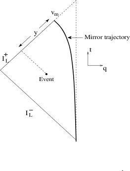
Figure 4: $y=|v-\ln 1/2\lambda|$ gives the coordinate distance between the projection of an event on ${\cal I}_{L}^{+}$ and the boundary on ${\cal I}_{L}^{+}$. At late time, since $q_{m}(t)\approx-t+\ln 1/2\lambda$, $y$ is same as the coordinate distance from the boundary.

so that at large $y$ both the above quantities fall off exponentially to the values corresponding to the static background.

Notice that the final results (5.112) very much depend on what regularization we work with. We shall now justify our regularization (5.96) by showing that in the region of validity of our analysis, it is consistent with the collective field theory counter term. The original derivation [38] of the collective field theory counter term (2.21) was formally background independent. This would imply that the counter term for the draining Fermi sea background will be given by,

$$\Delta H_{\lambda} = {g_{s}\over 2\sqrt{\pi}}\int_{-\infty}^{x_{m}(t)}dx~{}\partial_{x}\bar{\phi}_{0}^{(D)}(x,t)~{}\partial_{x}\partial_{x^{\prime}}\ln|x-x^{\prime}|_{x=x^{\prime}}~{},$$ (5.113)

$$= {1\over 2\pi}\int_{-\infty}^{x_{m}(t)}dx~{}P_{0}(x+\lambda e^{t})~{}\partial_{x}\partial_{x^{\prime}}\ln|x-x^{\prime}|_{x=x^{\prime}}~{}.$$ (5.114)

In the regularization (5.96) we have an undetermined function $\gamma(u,v)$. As long as we take $\lim_{v\to-\infty}\gamma(u,v)\to-1$ we recover both the singular and the finite parts of eq.(5.94) from eqs.(5.103). But for a Hamiltonian formulation it will be more natural to consider a spatial splitting. This requires us to take for all $u$ and $v$,

$$\gamma(u,v)=-1~{}.$$ (5.115)

With this one can compute ${\cal E}_{S}^{Coll}$ given in eqs.(5.103). To cancel this particular value of ${\cal E}_{S}^{Coll}$ one needs the following counter term,

$$(\Delta H_{\lambda})_{our}={1\over 2\pi}\int_{-\infty}^{x_{m}(t)}dx~{}\left\{{P_{0}(X)(1+h_{\lambda})\over P_{0}(x)}\right\}~{}{P_{0}(X)\over(\delta x)^{2}}~{}.$$ (5.116)

It is straightforward to check that the factor in the curly bracket simply reduces to $1$ in the region of validity giving the same result as (5.114).

6 Conclusion

The problem of particle production in the draining Fermi sea background of the two dimensional string theory was considered in [25] (see also [23]). In this paper the same problem has been reconsidered and analyzed in more detail. The basic accomplishments are the following:

1. Physical arguments have been given to establish that the Bogolubov analysis is sensible only in a limit where the deformation parameter $\lambda$ is small but nonzero.

2. An additional method of computing Bogolubov coefficients, namely the scattering method (which is very reminiscent of Polchinski’s wall scattering method [33] in the static background), has been presented.

3. The moving mirror method of computing the Bogolubov coefficients has been elaborated through the explicit construction of the natural out-modes. We show that the small $\lambda$ limit that has been considered on physical grounds is required to hold in order for both the above methods (which are quite independent) to work.

4. Time evolution of the energy-momentum tensor in the linearized approximation of the equation of motion has also been studied in detail. In [25] the coordinate transformation (3.30) (with $\lambda_{+}=\lambda~{},\lambda_{-}=0$) was taken to be,

   $$U=u~{},\quad V=v-\ln(1-2\lambda e^{v})~{},$$ (6.117)

   which is a conformal transformation. This, in fact, seems to be a good approximation on ${\cal I}_{L}^{+}$ (where $u\to\infty$) at a finite value of $\ln(1-2\lambda e^{v})$. The present work attempts to go beyond this approximation by incorporating the effect of the second term in the expression for $U$ in eq.(3.30). This term takes the transformation off the conformality giving a non-trivial effect on the metric (see eq.(4.57)).

   The present computations have been done with a metric (4.63) which is simpler than the actual one. This procedure gives rise to a reduced region of validity given by, (1) everywhere at early time, (2) large $|q|$ at a finite time and (3) finite $(1-2\lambda e^{v})$ at late time. Our computation is done in a particular regularization which leads to the certain singular term that is required to cancel the collective field theory counter term for the present background. As expected, this cancellation takes place only in the region of validity mentioned above.

   The final results show that the energy and momentum densities have non-trivial time evolution. They start up with constant values at early time but grows exponentially at late time as one approaches the boundary from a large distance. This clearly indicates radiation of energy due to the space-time decay. This is different from the result found in [25] where the densities remain constant as time evolves.

   Similar remarks apply to the result found in [24, 26]. The only difference between the treatments of [24] and [25] is that in [24] the initial value of $T_{vv}$ (which corresponds to the static background) was taken to be zero as opposed to the case of [25]. As a result [24] also finds exponential fall-off of the energy density. Although this is similar to the result found in this paper, the reasons are different.

Acknowledgment: I am thankful to S. R. Das for many discussions and various useful comments on the manuscript. I wish to thank J. Michelson and A. Shapere for enthusiastic questions and comments during a seminar delivered at the Department of Physics and Astronomy, University of Kentucky where the results of this paper were reported. I also thank A. Sen for his useful comments on the manuscript. This work was supported by National Science Foundation grant PHY-0244811 and the Department of Energy grant No. DE-FG01-00ER45832.

Appendix A Bogolubov Coefficients in Scattering Method

Here we give the details of the computation of the Bogolubov coefficients defined in eq.(4.36). Using eq.(4.37) with $\partial_{U}\Phi=0$, the coordinate transformation (3.30) with $\lambda_{+}=\lambda,~{}\lambda_{-}=0$ and the mode expansion for the field we get,

$$\int_{0}^{\infty}dw\sqrt{w}\left[A^{out}_{w}e^{-iwV}-h.c.\right] = \int_{0}^{\infty}dw\sqrt{w}\left[a^{out}_{w}{e^{-iwg_{\lambda}(V)}\over 1+2\lambda e^{V}}-h.c.\right]~{},$$ (A.1)

where we have introduced the function,

$$g_{\lambda}(x)=x-\ln(1+2\lambda e^{x})~{},\quad-\infty<x<\infty~{}.$$ (A.2)

Using the expansion (4.36) in eq.(A.1) and performing an indefinite integral over $V$ on both sides one gets,

$${1\over\sqrt{w}}e^{-iwV}=\int_{0}^{\infty}{dw^{\prime}\over\sqrt{w^{\prime}}}\left[\alpha(w^{\prime},w)e^{-iw^{\prime}g_{\lambda}(V)}+\beta^{*}(w^{\prime},w)e^{iw^{\prime}g_{\lambda}(V)}\right]$$ (A.3)

Introducing the function $f_{\lambda}(x)$, the inverse of $g_{\lambda}(x)$, as in eq.(4.40) we write the identity (A.3) as,

$${1\over\sqrt{w}}e^{-iwf_{\lambda}(x)}=\int_{0}^{\infty}{dw^{\prime}\over\sqrt{w^{\prime}}}\left[\alpha(w^{\prime},w)e^{-iw^{\prime}x}+\beta^{*}(w^{\prime},w)e^{iw^{\prime}x}\right]~{}.$$ (A.4)

Multiplying both sides by $e^{i\bar{w}x}$ and integrating over the valid range of $x$ (see eq.(4.40)) one gets,

$${1\over\sqrt{w}}\int_{-\infty}^{\ln 1/2\lambda}{dx\over 2\pi}e^{i\bar{w}x-iwf_{\lambda}(x)} = \int_{0}^{\infty}{dw^{\prime}\over\sqrt{w^{\prime}}}\left[\alpha(w^{\prime},w)I_{\lambda}(\bar{w}-w^{\prime})+\right.$$ (A.6)

$$\left.~{}~{}~{}~{}~{}~{}~{}~{}~{}~{}~{}~{}\beta^{*}(w^{\prime},w)I_{\lambda}(\bar{w}+w^{\prime})\right]~{},$$

where,

$$I_{\lambda}(w)=\int_{-\infty}^{\ln 1/2\lambda}{dx\over 2\pi}e^{iwx}~{},$$ (A.7)

which, in the small $\lambda$ limit, approaches $\delta(w)$. Approximating $I_{\lambda}(w)$ by $\delta(w)$ we get the coefficient $\alpha(\bar{w},w)$ from eq.(A.6). Similarly multiplying both sides of eq.(A.4) by $e^{-i\bar{w}x}$ and following the same steps one evaluates the coefficient $\beta(\bar{w},w)$. The results that one gets are given in eqs.(4.39).

Appendix B Geometrical Construction of the In and Out-Modes

In a moving mirror problem in flat space the natural in and out-modes have the following geometrical optics interpretation. Each of the two kinds of modes is a superposition of an incident and a reflected waves. The incident wave in an in-mode takes the simple plane-wave structure on ${\cal I}^{-}_{L}$, but the reflected one is complicated on ${\cal I}^{+}_{L}$. For an out-mode the incident part is complicated on ${\cal I}^{-}_{L}$ so that after reflection it takes the simple plane-wave form on ${\cal I}^{+}_{L}$. This means that if the metric (4.63) were flat the trajectory (4.64) would have corresponded to the following natural modes,

$$\phi^{in}_{w} = {1\over\sqrt{4\pi w}}\left[e^{-iwu}+s~{}e^{-iwp(v)}\right]\theta(q_{m}(t)-q)~{},\quad w\geq 0~{},$$ (B.1)

$$\phi^{out}_{w} = {1\over\sqrt{4\pi w}}\left[e^{-iwp^{-1}(u)}+s~{}e^{-iwv}\right]\theta(q_{m}(t)-q)~{},\quad w\geq 0~{},$$ (B.2)

where $p^{-1}(x)$ is the inverse function of $p(x)$ and $s=\mp$ correspond to the Dirichlet and Neumann boundary conditions respectively. We now try to generalize the above construction to our case through the following steps,

1. Find the two null directions $R_{\pm}^{\mu}(u,v)$ which can be found, up-to overall factors, by solving the following equations,

   $$R_{\pm}^{\mu}(u,v)R_{\pm\mu}(u,v)=0~{}.$$ (B.3)

   We get,

   $$R_{+}^{\mu}\sim(1~{},~{}~{}1-4\lambda e^{v})~{},\quad R_{-}^{\mu}\sim(1~{},~{}~{}-1)~{}.$$ (B.4)

   These give the structure of the light-cones (fig.5) in the given space.

   

   Figure 5: Curves with dot-style 1 and 2 are the null-rays whose tangent vectors are given by $R_{+}^{\mu}$ and $R_{-}^{\mu}$ respectively. Light-cones are same as that of a flat space on ${\cal I}^{-}_{L}$. They shrink as $v$ increases and are completely squeezed at $v=v_{m}=\ln 1/2\lambda$ where $R_{+}^{\mu}=R_{-}^{\mu}$.

   Since the metric becomes flat as $v\to-\infty$, the light-cones are stretched to $90^{\circ}$ cone-angle in that region. They shrink as $v$ increases and become completely squeezed at $v=v_{m}=\ln 1/2\lambda$ where a horizon is formed.

2. Find the null rays

   $$\xi(u,v)=\hbox{const.}\quad\zeta(u,v)=\hbox{const.}~{},$$ (B.5)

   i.e. the the curves which have $R_{\pm}^{\mu}(u,v)$ as tangent vectors respectively.

   $$R^{\mu}_{+}\partial_{\mu}\xi(u,v)=0~{},\quad R^{\mu}_{-}\partial_{\mu}\zeta(u,v)=0~{}.$$ (B.6)

   The two null coordinates are found to be,

   $$\xi(u,v)=u+\ln(1-2\lambda e^{v})~{},\quad\zeta(u,v)=v$$ (B.7)

3. Generalize eqs.(B.2) by the following,

   $$\phi^{in}_{w} = {1\over\sqrt{4\pi w}}\left[e^{-iw\xi}+s~{}e^{-iwf(\zeta)}\right]\theta(q_{m}(t)-q)~{},\quad w\geq 0~{},$$ (B.8)

   $$\phi^{out}_{w} = {1\over\sqrt{4\pi w}}\left[e^{-iwg(\xi)}+s~{}e^{-iw\zeta}\right]\theta(q_{m}(t)-q)~{},\quad w\geq 0~{},$$ (B.9)

   where the functions $f(x)$ and $g(x)$ are inverse of each other. $f(x)$ appears in the equation of the trajectory in the $(\xi,\zeta)$ coordinates in the following way,

   $$\xi=f(\zeta)~{}.$$ (B.10)

   It is straightforward to check that the functions $e^{iw\xi(u,v)}$ and $e^{iw\zeta(u,v)}$ are the two independent solutions of the Klein-Gordon field equation in the given metric. In our case the functions $f(x)$ and $g(x)$ appearing in eqs.(B.9) turn out to be $f_{\lambda}(x)$ and $g_{\lambda}(x)$ introduced in eqs.(4.40) and (A.2) respectively so that the modes take the final form as shown in eqs.(4.66).

Appendix C Point-splitting Regularization in the Draining Fermi Sea Background

It will be useful for our purpose to work in the $(u,v)$ coordinate system. The metric in this system is given by,

$${\bf g}_{ab}={1\over 2}\left(\begin{array}[]{cc}0&f^{\prime}_{\lambda}(v)\\ f^{\prime}_{\lambda}(v)&-4\lambda e^{v}f^{\prime}_{\lambda}(v)^{2}\end{array}\right)~{},\quad{\bf g}^{ab}=2\left(\begin{array}[]{cc}4\lambda e^{v}&{1\over f^{\prime}_{\lambda}(v)}\\ {1\over f^{\prime}_{\lambda}(v)}&0\end{array}\right)~{},$$ (C.15)

where $a,b=u,v$. We get,

$$T=8\lambda e^{v}\partial_{u}\phi\partial_{u}\phi+{2\over f^{\prime}_{\lambda}(v)}\partial_{u}\phi\partial_{v}\phi+{2\over f^{\prime}_{\lambda}(v)}\partial_{v}\phi\partial_{u}\phi~{}.$$ (C.16)

Here we are distinguishing $\partial_{u}\phi\partial_{v}\phi$ from $\partial_{v}\phi\partial_{u}\phi$ as we shall consider a point-splitting regularization of the operators. The components of the stress-tensor in the $(u,v)$ system turn out to be,

$$T_{uu} = \partial_{u}\phi\partial_{u}\phi~{},$$ (C.17)

$$T_{vv} = \partial_{v}\phi\partial_{v}\phi+2h_{\lambda}(v)^{2}\partial_{u}\phi\partial_{u}\phi+h_{\lambda}(v)\left(\partial_{u}\phi\partial_{v}\phi+\partial_{v}\phi\partial_{u}\phi\right)~{},$$ (C.18)

$$T_{uv} = {1\over 2}\left(\partial_{u}\phi\partial_{v}\phi-\partial_{v}\phi\partial_{u}\phi\right)-h_{\lambda}(v)\partial_{u}\phi\partial_{u}\phi~{},$$ (C.19)

$$T_{vu} = -{1\over 2}(\partial_{u}\phi\partial_{v}\phi-\partial_{v}\phi\partial_{u}\phi)-h_{\lambda}(v)\partial_{u}\phi\partial_{u}\phi~{},$$ (C.20)

where $h_{\lambda}(v)$ has been defined in eqs.(5.87). At early time ($v\to-\infty\Rightarrow h_{\lambda}(v)\to 0$) we recover the standard results for flat space. The vacuum expectation values can be written in terms of the basic objects,

$$D_{ab}(u,v)\equiv\langle\partial_{a}\phi\partial_{b}\phi\rangle~{}.$$ (C.21)

For explicit computation we expand $\phi$ in terms of the in-modes. Then we point-split $D_{ab}(u,v)$ in the following way,

$$D_{ab}(u,v)=\lim_{\delta u,\delta v\to 0}\int_{0}^{\infty}dw~{}\partial_{a_{1}}\phi^{in}_{w}(u_{1},v_{1})\partial_{b_{2}}\phi^{in*}_{w}(u_{2},v_{2})~{},$$ (C.22)

where the point-splitting is taken to be symmetrical (5.77). Using the full in-modes given in eqs.(4.66) and the result $\int_{0}^{\infty}dw~{}we^{iwx}=-{1\over x^{2}}$ one gets,

$$D_{uu} = -{1\over 4\pi(\delta\xi)^{2}}~{},\quad\delta\xi=\xi_{2}-\xi_{1}~{},$$ (C.23)

$$D_{vv} = -{h_{\lambda}(v_{1})h_{\lambda}(v_{2})\over 4\pi(\delta\xi)^{2}}-{f^{\prime}_{\lambda}(v_{1})f^{\prime}_{\lambda}(v_{2})\over 4\pi\left(f_{\lambda}(v_{1})-f_{\lambda}(v_{2})\right)^{2}}+{s\over 4\pi}\left[{h_{\lambda}(v_{1})f^{\prime}_{\lambda}(v_{2})\over(f_{\lambda}(v_{2})-\xi_{1})^{2}}+{h_{\lambda}(v_{2})f^{\prime}_{\lambda}(v_{1})\over(f_{\lambda}(v_{1})-\xi_{2})^{2}}\right]~{},$$ (C.24)

$$D_{uv} = {h_{\lambda}(v_{2})\over 4\pi(\delta\xi)^{2}}-{s\over 4\pi}\left[{f^{\prime}_{\lambda}(v_{2})\over(\xi_{1}-f_{\lambda}(v_{2}))^{2}}\right]~{},$$ (C.25)

$$D_{vu} = {h_{\lambda}(v_{1})\over 4\pi(\delta\xi)^{2}}-{s\over 4\pi}\left[{f^{\prime}_{\lambda}(v_{1})\over(f_{\lambda}(v_{1})-\xi_{2})^{2}}\right]~{}.$$ (C.26)

Notice that the terms in the square brackets do not have any short distance divergence. Moreover, because of the factor in the denominator, they are suppressed both at late time and at a finite time but large $|q|$. Therefore we shall simply drop these terms. The rest of the terms are computed, using the identity (5.93), to be,

$$D_{ab} = S_{ab}+F_{ab}~{},$$ (C.27)

where the singular and finite terms $S_{ab}$ and $F_{ab}$ respectively are given by,

$$S_{uu} = -{1\over 4\pi(\gamma-h_{\lambda})^{2}(\delta v)^{2}}~{},$$ (C.28)

$$S_{vv} = -{h_{\lambda}^{2}\over 4\pi(\gamma-h_{\lambda})^{2}(\delta v)^{2}}-{1\over 4\pi(\delta v)^{2}}~{},$$ (C.29)

$$S_{uv} = {h_{\lambda}\over 4\pi(\gamma-h_{\lambda})^{2}(\delta v)^{2}}+{h_{\lambda}^{\prime}\over 8\pi(\gamma-h_{\lambda})^{2}\delta v}~{},$$ (C.30)

$$S_{vu} = {h_{\lambda}\over 4\pi(\gamma-h_{\lambda})^{2}(\delta v)^{2}}-{h_{\lambda}^{\prime}\over 8\pi(\gamma-h_{\lambda})^{2}\delta v}~{},$$ (C.31)

$$F_{uu} = -{\psi(h_{\lambda})\over 2\pi(\gamma-h_{\lambda})^{3}}~{},$$ (C.32)

$$F_{vv} = -{h_{\lambda}^{2}\psi(h_{\lambda})\over 2\pi(\gamma-h_{\lambda})^{3}}-{h_{\lambda}h_{\lambda}^{\prime\prime}-(h_{\lambda}^{\prime})^{2}\over 16\pi(\gamma-h_{\lambda})^{2}}-{S(f_{\lambda},v)\over 24\pi}~{},$$ (C.33)

$$F_{uv} = F_{vu}={h_{\lambda}\psi(h_{\lambda})\over 2\pi(\gamma-h_{\lambda})^{3}}+{h_{\lambda}^{\prime\prime}\over 32\pi(\gamma-h_{\lambda})^{2}}~{},$$ (C.34)

where $\psi(h_{\lambda})$ is given in eqs.(5.87). $h_{\lambda}$ appearing on the right hand sides of all the above equations is meant to be evaluated at $v$. We have also used eq.(5.84). These results and the standard transformation laws of stress-tensor components under the coordinate transformation $(u,v)\to(t,q)$ allow us to finally compute $\langle T_{\mu\nu}\rangle$. The results are,

$$\langle T_{\mu\nu}\rangle=\langle T_{\mu\nu}\rangle_{S}+\langle T_{\mu\nu}\rangle_{F}~{},$$ (C.35)

where the singular and finite parts $\langle T_{\mu\nu}\rangle_{S}$ and $\langle T_{\mu\nu}\rangle_{F}$ respectively are given by,

$$\langle T_{00}\rangle_{S} = -{1\over 4\pi(\delta v)^{2}}\left[1+\left({1-h_{\lambda}\over\gamma-h_{\lambda}}\right)^{2}\right]~{},$$ (C.36)

$$\langle T_{11}\rangle_{S} = -{1\over 4\pi(\delta v)^{2}}\left[1+\left({1+h_{\lambda}\over\gamma-h_{\lambda}}\right)^{2}\right]~{},$$ (C.37)

$$\langle T_{01}\rangle_{S} = -{1\over 4\pi(\delta v)^{2}}\left[1-{1-h_{\lambda}^{2}\over(\gamma-h_{\lambda})^{2}}\right]+{h_{\lambda}^{\prime}\over 4\pi\delta v(\gamma-h_{\lambda})^{2}}~{},$$ (C.38)

$$\langle T_{10}\rangle_{S} = -{1\over 4\pi(\delta v)^{2}}\left[1-{1-h_{\lambda}^{2}\over(\gamma-h_{\lambda})^{2}}\right]-{h_{\lambda}^{\prime}\over 4\pi\delta v(\gamma-h_{\lambda})^{2}}~{},$$ (C.39)

$$\langle T_{00}\rangle_{F} = -{\psi(h_{\lambda})(1-h_{\lambda})^{2}\over 2\pi(\gamma-h_{\lambda})^{3}}+{(h_{\lambda}^{\prime})^{2}\over 16\pi(\gamma-h_{\lambda})^{2}}-{S(f_{\lambda},v)\over 24\pi}~{},$$ (C.40)

$$\langle T_{11}\rangle_{F} = -{\psi(h_{\lambda})(1+h_{\lambda})^{2}\over 2\pi(\gamma-h_{\lambda})^{3}}+{(h_{\lambda}^{\prime})^{2}\over 16\pi(\gamma-h_{\lambda})^{2}}-{S(f_{\lambda},v)\over 24\pi}~{},$$ (C.41)

$$\langle T_{01}\rangle_{F} = \langle T_{10}\rangle_{F}={\psi(h_{\lambda})(1-h_{\lambda}^{2})\over 2\pi(\gamma-h_{\lambda})^{3}}+{(h_{\lambda}^{\prime})^{2}\over 16\pi(\gamma-h_{\lambda})^{2}}-{S(f_{\lambda},v)\over 24\pi}~{}.$$ (C.42)

Notice that each of $\langle T_{01}\rangle_{S}$ and $\langle T_{10}\rangle_{S}$ has a linearly divergent term which comes from the similar terms in $S_{uv}$ and $S_{vu}$ given in eqs.(C.31).

Appendix D Relation between Bogolubov and Stress-Tensor Analysis

Some part of $\langle T_{\mu\nu}\rangle_{R}$ can, in fact, be written in terms of the Bogolubov coefficients $\alpha(w,w^{\prime})$ and $\beta(w,w^{\prime})$. Following [44] we expand the right hand side of eq.(C.21) in terms of the out-modes and use the unitarity properties of the Bogolubov coefficients to get,

$$D_{ab} = D^{out}_{ab}+B_{ab}~{},$$ (D.43)

$$B_{ab} = B^{(\rho)}_{ab}+B^{(\mu)}_{ab}~{},$$ (D.44)

where

$$D^{out}_{ab} = \int_{0}^{\infty}dw~{}\partial_{a}\phi^{out}_{w}\partial_{b}\phi^{out*}_{w}~{},$$ (D.45)

$$B^{(\rho)}_{ab} = 2\left[\int_{0}^{\infty}dw_{1}dw_{2}~{}\partial_{a}\phi^{out}_{w_{1}}\partial_{b}\phi^{out*}_{w_{2}}\rho_{\lambda}(w_{1},w_{2})\right]~{},$$ (D.46)

$$B^{(\mu)}_{ab} = 2\hbox{Re}\left[\int_{0}^{\infty}dw_{1}dw_{2}~{}\partial_{a}\phi^{out}_{w_{1}}\partial_{b}\phi^{out*}_{w_{2}}\mu_{\lambda}(w_{1},w_{2})\right]~{},$$ (D.47)

$$\rho_{\lambda}(w_{1},w_{2}) = \int_{0}^{\infty}dw\beta(w_{1},w)\beta^{*}(w_{2},w)~{},$$ (D.48)

$$\mu_{\lambda}(w_{1},w_{2}) = \int_{0}^{\infty}dw\beta(w_{1},w)\alpha(w_{2},w)~{}.$$ (D.49)

Proceeding in the same way as the one that leads to eqs.(C.27) one can compute $D^{out}_{ab}$. Subtracting this off from $D_{ab}$ given in eqs.(C.27) one gets $B_{ab}$. The answers that one gets are the following,

$$B_{uu} = {1\over 24\pi}S(g_{\lambda},\xi)=-{1\over 48\pi}~{},$$ (D.50)

$$B_{vv} = {h_{\lambda}^{2}\over 24\pi}S(g_{\lambda},\xi)-{1\over 24\pi}S(f_{\lambda},v)=-{h_{\lambda}^{2}\over 48\pi}-{1\over 24\pi}S(f_{\lambda},v)~{},$$ (D.51)

$$B_{uv} = B_{vu}=-{h_{\lambda}\over 24\pi}S(g_{\lambda},\xi)={h_{\lambda}\over 48\pi}~{},$$ (D.52)

where we have taken the large time limit ($\lim_{u\to\infty}S(g_{\lambda},\xi)\to-1/2$) in the above expressions. Notice that $B_{ab}$ can also be computed using eqs.(D.44) and (D.49) in terms of the Bogolubov coefficients. This requires some particular integrals of these coefficients to be equal to functions appearing on the right hand side of eq.(D.52). It can be explicitly checked that all such relations can be satisfied by the following single equality.

$$I^{(\rho)}_{\lambda}(v)+I^{(\mu)}_{\lambda}(v) = -{1\over 12}S(f_{\lambda},v)~{},$$ (D.53)

where,

$$I^{(\rho)}_{\lambda}(v) = \int_{0}^{\infty}dw_{1}dw_{2}\sqrt{w_{1}w_{2}}e^{i(w_{2}-w_{1})v}\rho_{\lambda}(w_{1},w_{2})~{},$$ (D.54)

$$I^{(\mu)}_{\lambda}(v) = \hbox{Re}\left[\int_{0}^{\infty}dw_{1}dw_{2}\sqrt{w_{1}w_{2}}e^{i(w_{2}-w_{1})v}\mu_{\lambda}(w_{1},w_{2})\right]~{}.$$ (D.55)

For genuine Bogolubov coefficients satisfying the unitarity conditions the above relation must be true. Our Bogolubov coefficients given in eqs.(LABEL:bogol-II) are approximately correct for small $\lambda$. Although we have not quite succeeded, we attempted to understand how far the equality (D.53) can be satisfied by our Bogolubov coefficients. Below we shall report on how far we have been able to go.

Using the variable $y$ (5.111) one can erase the appearance of $\lambda$ on the right hand side of (D.53).

$$S(f_{\lambda},v)=-\partial_{y}\tilde{h}(y)-{1\over 2}\tilde{h}(y)^{2}~{}.$$ (D.56)

This means that it should be possible to fully absorb the $\lambda$ and $v$ dependence of $(I^{(\rho)}_{\lambda}(v)+I^{(\mu)}_{\lambda}(v))$ into $y$. Using the $\alpha$ and $\beta$ coefficients in (LABEL:bogol-II) one can readily check that it really happens for $I^{(\rho)}_{\lambda}(v)$,

$$I^{(\rho)}(y) := I^{(\rho)}_{\lambda}(v)={1\over 4\pi}\int_{0}^{\infty}dw_{1}dw_{2}~{}{e^{i(w_{1}-w_{2})y}\over\Gamma(iw_{1})\Gamma(-iw_{2})}\int_{0}^{\infty}dw{\Gamma(i(w_{1}+w))\Gamma(-i(w_{2}+w))\over\sinh\pi w}~{},$$ (D.57)

but not quite for $I^{(\mu)}_{\lambda}(v)$,

$$I^{(\mu)}_{\lambda}(v) = -{1\over 4\pi}\hbox{Re}\left[\int_{0}^{\infty}dw_{1}dw_{2}e^{i(w_{1}-w_{2})y}{\Gamma(i(w_{1}+w_{2}))\Gamma(iw_{2})\over\Gamma(iw_{1})}\left\{w_{2}e^{2iw_{2}\ln 1/2\lambda}\right\}\right]$$ (D.60)

$$-{1\over 4\pi}\hbox{Re}\left[\int_{0}^{\infty}dwdw_{1}dw_{2}e^{i(w_{1}-w_{2})y}{\Gamma(i(w_{1}+w))\Gamma(i(w_{2}+w))\over\Gamma(iw_{1})\Gamma(1+iw_{2})\sinh\pi w}i\left\{w_{2}e^{2iw_{2}\ln 1/2\lambda}\right\}\right]~{},$$

Notices that because of the factor kept in the curly brackets in the above expression one can set, for small $\lambda$,

$$I^{(\mu)}_{\lambda}(v)=0~{},$$ (D.62)

so that one is left with the identity,

$$I^{(\rho)}(y)={1\over 12}\partial_{y}\tilde{h}(y)+{1\over 24}\tilde{h}(y)^{2}~{}.$$ (D.63)

It has not been possible for us to check this identity either analytically or numerically.

References

-
[1]
J. Polchinski,
“String Theory. Vol. 1: An Introduction To The Bosonic String,”
“String Theory. Vol. 2: Superstring Theory And Beyond,”
“What is string theory?,” arXiv:hep-th/9411028. - [2] I. R. Klebanov, “String theory in two-dimensions,” arXiv:hep-th/9108019.
- [3] P. H. Ginsparg and G. W. Moore, “Lectures On 2-D Gravity And 2-D String Theory,” arXiv:hep-th/9304011.
- [4] A. Jevicki, “Development in 2-d string theory,” arXiv:hep-th/9309115.
- [5] E. Brezin, C. Itzykson, G. Parisi and J. B. Zuber, “Planar Diagrams,” Commun. Math. Phys. 59, 35 (1978). D. J. Gross and N. Miljkovic, “A Nonperturbative Solution Of D = 1 String Theory,” Phys. Lett. B 238, 217 (1990). E. Brezin, V. A. Kazakov and A. B. Zamolodchikov, “Scaling Violation In A Field Theory Of Closed Strings In One Physical Nucl. Phys. B 338, 673 (1990). P. H. Ginsparg and J. Zinn-Justin, “2-D Gravity + 1-D Matter,” Phys. Lett. B 240, 333 (1990).
- [6] T. Takayanagi and N. Toumbas, “A matrix model dual of type 0B string theory in two dimensions,” JHEP 0307, 064 (2003) [arXiv:hep-th/0307083].
- [7] M. R. Douglas, I. R. Klebanov, D. Kutasov, J. Maldacena, E. Martinec and N. Seiberg, “A new hat for the c = 1 matrix model,” arXiv:hep-th/0307195.
- [8] H. Dorn and H. J. Otto, “On correlation functions for noncritical strings with c 1 d 1,” Phys. Lett. B 291, 39 (1992) [arXiv:hep-th/9206053].
- [9] H. Dorn and H. J. Otto, “Two and three point functions in Liouville theory,” Nucl. Phys. B 429, 375 (1994) [arXiv:hep-th/9403141].
- [10] A. B. Zamolodchikov and A. B. Zamolodchikov, “Structure constants and conformal bootstrap in Liouville field theory,” Nucl. Phys. B 477, 577 (1996) [arXiv:hep-th/9506136].
- [11] J. Teschner, “Liouville theory revisited,” Class. Quant. Grav. 18, R153 (2001) [arXiv:hep-th/0104158].
-
[12]
A. B. Zamolodchikov and A. B. Zamolodchikov,
“Liouville field theory on a pseudosphere,”
arXiv:hep-th/0101152.
T. Fukuda and K. Hosomichi, “Super Liouville theory with boundary,” Nucl. Phys. B 635, 215 (2002) [arXiv:hep-th/0202032].
C. Ahn, C. Rim and M. Stanishkov, “Exact one-point function of N = 1 super-Liouville theory with boundary,” Nucl. Phys. B 636, 497 (2002) [arXiv:hep-th/0202043]. - [13] E. J. Martinec, “The annular report on non-critical string theory,” arXiv:hep-th/0305148.
- [14] S. Y. Alexandrov, V. A. Kazakov and D. Kutasov, “Non-perturbative effects in matrix models and D-branes,” JHEP 0309, 057 (2003) [arXiv:hep-th/0306177].
- [15] J. McGreevy and H. Verlinde, “Strings from tachyons: The c = 1 matrix reloaded,” JHEP 0312, 054 (2003) [arXiv:hep-th/0304224].
- [16] I. R. Klebanov, J. Maldacena and N. Seiberg, “D-brane decay in two-dimensional string theory,” JHEP 0307, 045 (2003) [arXiv:hep-th/0305159].
- [17] A. Sen, “Open-closed duality: Lessons from matrix model,” Mod. Phys. Lett. A 19, 841 (2004) [arXiv:hep-th/0308068].
- [18] V. Schomerus, “Rolling tachyons from Liouville theory,” JHEP 0311, 043 (2003) [arXiv:hep-th/0306026]. D. Gaiotto, N. Itzhaki and L. Rastelli, “On the BCFT description of holes in the c = 1 matrix model,” Phys. Lett. B 575, 111 (2003) [arXiv:hep-th/0307221]. M. Gutperle and P. Kraus, “D-brane dynamics in the c = 1 matrix model,” Phys. Rev. D 69, 066005 (2004) [arXiv:hep-th/0308047]. O. DeWolfe, R. Roiban, M. Spradlin, A. Volovich and J. Walcher, “On the S-matrix of type 0 string theory,” JHEP 0311, 012 (2003) [arXiv:hep-th/0309148]. S. Dasgupta and T. Dasgupta, “Renormalization group approach to c = 1 matrix model on a circle and D-brane arXiv:hep-th/0310106. D. J. Gross and J. Walcher, “Non-perturbative RR potentials in the c(hat) = 1 matrix model,” arXiv:hep-th/0312021. J. de Boer, A. Sinkovics, E. Verlinde and J. T. Yee, “String interactions in c = 1 matrix model,” JHEP 0403, 023 (2004) [arXiv:hep-th/0312135]. J. Ambjorn and R. A. Janik, “The decay of quantum D-branes,” Phys. Lett. B 584, 155 (2004) [arXiv:hep-th/0312163]. G. Mandal and S. R. Wadia, “Rolling tachyon solution of two-dimensional string theory,” arXiv:hep-th/0312192. S. R. Das, “D branes in 2d string theory and classical limits,” arXiv:hep-th/0401067. A. Sen, “Rolling tachyon boundary state, conserved charges and two dimensional string theory,” arXiv:hep-th/0402157. T. Takayanagi, “Notes on D-branes in 2D type 0 string theory,” arXiv:hep-th/0402196.
-
[19]
A. Sen,
“Rolling tachyon,”
JHEP 0204, 048 (2002)
[arXiv:hep-th/0203211].
A. Sen, “Tachyon matter,” JHEP 0207, 065 (2002) [arXiv:hep-th/0203265]. - [20] D. Minic, J. Polchinski and Z. Yang, “Translation Invariant Backgrounds In (1+1)-Dimensional String Theory,” Nucl. Phys. B 369, 324 (1992).
- [21] G. W. Moore and R. Plesser, “Classical scattering in (1+1)-dimensional string theory,” Phys. Rev. D 46, 1730 (1992) [arXiv:hep-th/9203060].
- [22] S. Y. Alexandrov, V. A. Kazakov and I. K. Kostov, “Time-dependent backgrounds of 2D string theory,” Nucl. Phys. B 640, 119 (2002) [arXiv:hep-th/0205079].
- [23] J. L. Karczmarek and A. Strominger, “Matrix cosmology,” arXiv:hep-th/0309138.
- [24] J. L. Karczmarek and A. Strominger, “Closed string tachyon condensation at c = 1,” arXiv:hep-th/0403169.
- [25] S. R. Das, J. L. Davis, F. Larsen and P. Mukhopadhyay, “Particle production in matrix cosmology,” arXiv:hep-th/0403275.
- [26] J. L. Karczmarek, A. Maloney and A. Strominger, “Hartle-Hawking vacuum for c = 1 tachyon condensation,” arXiv:hep-th/0405092.
- [27] M. Ernebjerg, J. L. Karczmarek and J. M. Lapan, “Collective field description of matrix cosmologies,” arXiv:hep-th/0405187.
- [28] D. J. Gross and I. R. Klebanov, “S = 1 for c = 1,” Nucl. Phys. B 359, 3 (1991).
- [29] G. W. Moore, “Double scaled field theory at c = 1,” Nucl. Phys. B 368, 557 (1992).
-
[30]
K. Demeterfi, A. Jevicki and J. P. Rodrigues,
“Scattering amplitudes and loop corrections in collective string field
theory,”
Nucl. Phys. B 362, 173 (1991).
K. Demeterfi, A. Jevicki and J. P. Rodrigues, “Scattering amplitudes and loop corrections in collective string field theory. 2,” Nucl. Phys. B 365, 499 (1991).
K. Demeterfi, A. Jevicki and J. P. Rodrigues, “Perturbative results of collective string field theory,” Mod. Phys. Lett. A 6, 3199 (1991). -
[31]
A. M. Sengupta and S. R. Wadia,
“Excitations And Interactions In D = 1 String Theory,”
Int. J. Mod. Phys. A 6, 1961 (1991).
G. Mandal, A. M. Sengupta and S. R. Wadia, “Interactions and scattering in d = 1 string theory,” Mod. Phys. Lett. A 6, 1465 (1991). - [32] P. Di Francesco and D. Kutasov, “Correlation functions in 2-D string theory,” Phys. Lett. B 261, 385 (1991).
- [33] J. Polchinski, “Classical Limit Of (1+1)-Dimensional String Theory,” Nucl. Phys. B 362, 125 (1991).
- [34] J. Polchinski, “On the nonperturbative consistency of d = 2 string theory,” Phys. Rev. Lett. 74, 638 (1995) [arXiv:hep-th/9409168].
-
[35]
N. Seiberg,
“Notes On Quantum Liouville Theory And Quantum Gravity,”
Prog. Theor. Phys. Suppl. 102, 319 (1990).
- [36] J. Polchinski, “Remarks On The Liouville Field Theory,” UTTG-19-90 Presented at Strings ’90 Conf., College Station, TX, Mar 12-17, 1990
- [37] A. Jevicki and B. Sakita, “The Quantum Collective Field Method And Its Application To The Planar Nucl. Phys. B 165, 511 (1980).
- [38] I. Andric and V. Bardek, “1/N Corrections In The Matrix Model And The Quantum Collective Field,” Phys. Rev. D 32, 1025 (1985).
- [39] S. R. Das and A. Jevicki, “String Field Theory And Physical Interpretation Of D = 1 Strings,” Mod. Phys. Lett. A 5, 1639 (1990).
- [40] D. J. Gross and I. R. Klebanov, “Fermionic String Field Theory Of C = 1 Two-Dimensional Quantum Gravity,” Nucl. Phys. B 352, 671 (1991).
- [41] A. M. Polyakov, “Selftuning Fields And Resonant Correlations In 2-D Gravity,” Mod. Phys. Lett. A 6, 635 (1991).
- [42] B. S. Dewitt, “Quantum Field Theory In Curved Space-Time,” Phys. Rept. 19, 295 (1975).
- [43] P. C. W. Davies and S. A. Fulling, “Radiation From A Moving Mirror In Two-Dimensional Space-Time Conformal Proc. Roy. Soc. Lond. A 348, 393 (1976).
- [44] P. C. W. Davies and S. A. Fulling, “Radiation From Moving Mirrors And From Black Holes,” Proc. Roy. Soc. Lond. A 356, 237 (1977).
- [45] N. D. Birrell and P. C. W. Davies, “Quantum Fields In Curved Space,”
- [46] R. M. Wald, “General Relativity,”
- [47] S. W. Hawking, “Particle Creation By Black Holes,” Commun. Math. Phys. 43, 199 (1975).
- [48] J. Polchinski, “Critical Behavior Of Random Surfaces In One-Dimension,” Nucl. Phys. B 346, 253 (1990).
-
[49]
J. Avan and A. Jevicki,
“Classical integrability and higher symmetries of collective string field
theory,”
Phys. Lett. B 266, 35 (1991).
E. Witten, “Ground ring of two-dimensional string theory,” Nucl. Phys. B 373, 187 (1992) [arXiv:hep-th/9108004]. G. W. Moore and N. Seiberg, “From loops to fields in 2-D quantum gravity,” Int. J. Mod. Phys. A 7 (1992) 2601.
S. R. Das, A. Dhar, G. Mandal and S. R. Wadia, “Gauge theory formulation of the C = 1 matrix model: Symmetries and discrete states,” Int. J. Mod. Phys. A 7, 5165 (1992) [arXiv:hep-th/9110021].
S. R. Das, A. Dhar, G. Mandal and S. R. Wadia, “W infinity ward identities and correlation functions in the C = 1 matrix model,” Mod. Phys. Lett. A 7, 937 (1992) [Erratum-ibid. A 7, 2245 (1992)] [arXiv:hep-th/9112052].