By analytically continuing recently-found instantons we construct time-dependent solutions of Einstein-Maxwell de Sitter gravity which smoothly bounce between two de Sitter phases. These deformations of de Sitter space undergo several stages in their time evolution. Four and five-dimensional de Sitter bounces can be lifted to non-singular time-dependent solutions of M-theory.

1 Introduction

Cosmological bounces may provide an alternative to inflation, in terms of addressing the homogeneity problem and providing a causal mechanism of structure formation. Instead of an inflationary phase of quasi-exponential expansion, a bounce could have a long period of slow contraction, during which currently observed cosmological scales would be well inside the Hubble radius. Then, for example, there would be ample time for the observed homogeneity to occur through causal microphysics.

String-based models, such as Pre-Big-Bang cosmology [2, 4] and the Ekpyrotic scenario [6], have led to an increased interest in cosmological bounces. In fact, it was long believed that stringy corrections and quantum loop effects were required to smooth a cosmological singularity out to a smooth bounce [8]. This was reinforced when cosmological solutions were later found which turned out to all be singular [10, 12, 14, 16]; these solutions are now generally classified as S(pacelike)-branes [18].

The construction of classical non-singular time-dependent solutions is therefore of interest. One approach to resolve a cosmological singularity is for the cosmological flow to connect early and late-time de Sitter spacetimes [20]. It has been found in [22, 24] that AdS black holes can be analytically continued to non-singular cosmological solutions. In four dimensions, the resulting time-dependent solution smoothly interpolates between dS${}_{2}\times S^{2}$ and a dS₄-type geometry with a boundary of $S^{2}\times S^{1}$. These solutions are not supersymmetric, although a subset solves the first-order equations that coincide with the BPS equations for a non-compact $R$-symmetry. Also, these solutions are in a minimum of the potential with no tachyonic directions. This indicates that these smooth cosmological solutions may be stable [20]. The more general class of these solutions arise from the second-order equations of motion and can be fine-tuned to describe an expanding universe whose expansion rate is significantly larger in the past than in the future, providing a cosmological model with no singularities. These four-dimensional solutions have been lifted to non-singular S-brane configurations in eleven dimensions [26, 28].

More recently, non-singular S-branes have also been shown to arise from the analytical continuation of diholes [30], Kerr black holes [32, 34] and rotating $p$-branes [36]. Generically these solutions either smoothly interpolate from a warped product of two-dimensional de Sitter spacetime and an internal space to Minkowski spacetime, or smoothly bounce between two phases of Minkowski spacetime. These solutions explicitly demonstrate that certain cosmological singularities can be smoothed out to yield smooth bounces without the inclusion of stringy or quantum effects. Also unlike the resolution of p-brane singularities, which tend to require additional flux fields [38], these cosmological bounces rely only on classical gravitational physics and not matter fields.

In constructing a cosmological bounce model, it is important to take into account the late-time behavior. Astrophysical evidence suggests that our universe is currently in a de Sitter phase [40, 42]. In this paper, we construct de Sitter bounces by analytically continuing the de Sitter instantons found in [44]. In certain cases, we find that the four-dimensional de Sitter bounce satisfies BPS constraints, which implies that the solution might be stable. Interestingly, the bounce can also be fine-tuned to reduce the effect of the cosmological constant for an intermediate period of time, which might result in a longer period of slow contraction. In this case, the cosmological bounce could be an alternative to inflation.

The rest of this paper is organized as follows. In the next section, we analytically continue de Sitter instantons to time-dependent solutions which smoothly bounce between two de Sitter phases. In section 3, we generalize the four-dimensional de Sitter bounce to include electric and magnetic charges. This solution can be analytically continued from an AdS Reissner-Nördstrom Taub-NUT solution. In section 4, we lift the four and five-dimensional de Sitter bounces to eleven-dimensional supergravity and type IIB theory, respectively. Conclusions are presented in section 5.

2 From instantons to bounces

We begin with the recently-discussed instanton solutions to Euclidean de Sitter gravity, found in [44]

$$ds_{d}^{2}=\frac{(1-r^{2})^{n}}{P(r)}\,dr^{2}+\frac{c^{2}\,P(r)}{(1-r^{2})^{n}}\,(d\psi-2A)^{2}+c\,(1-r^{2})\,d\Sigma_{2n}^{2}+\frac{m-1}{\Lambda-\lambda\,c^{-1}}\,r^{2}\,d\Omega_{m}^{2},$$ (2.1)

where $c$ is an arbitrary integration constant, $\lambda$ is the cosmological constant of the $2n$-dimensional Einstein-Kähler space $\Sigma_{2n}$ with the metric $d\Sigma_{2n}^{2}$ and $\Lambda$ is the cosmological constant of the $d=2n+m+2$-dimensional metric $ds_{d}^{2}$. After rescaling, these constants only appear in the dimensionless combination

$$\nu\equiv\frac{c\,\Lambda}{\lambda}\,.$$ (2.2)

In our notation, $d\Omega_{m}^{2}$ is the metric of a unit sphere $S^{m}$ and $A$ is the potential for the Kähler form on $d\Sigma_{2n}^{2}$, such that the Kähler two-form is given as $J=dA$. The function $P(r)$ is given by

$$P(r)=\frac{\Lambda}{m-1}\,_{2}F_{1}(-n-1,{\textstyle{\frac{\scriptstyle m-1}{\scriptstyle 2}}};{\textstyle{\frac{\scriptstyle m+1}{\scriptstyle 2}}};r^{2})-\frac{\lambda\,c^{-1}}{m-1}\,_{2}F_{1}(-n,{\textstyle{\frac{\scriptstyle m-1}{\scriptstyle 2}}};{\textstyle{\frac{\scriptstyle m+1}{\scriptstyle 2}}};r^{2})+\mu\,r^{1-m}\,,$$ (2.3)

where ${}_{2}F_{1}$ denotes the standard hypergeometric function. The parameter $\mu$ is an integration constant. Additional details of this solution can be found in [44]. For easy reference, we write the first few hypergeometric functions explicitly as polynomials in $r$:

$${}_{2}F_{1}(-1,{\textstyle{\frac{\scriptstyle m-1}{\scriptstyle 2}}};{\textstyle{\frac{\scriptstyle m+1}{\scriptstyle 2}}};r^{2}) = \frac{1}{m-1}-\frac{r^{2}}{m+1}$$ (2.4)

$${}_{2}F_{1}(-2,{\textstyle{\frac{\scriptstyle m-1}{\scriptstyle 2}}};{\textstyle{\frac{\scriptstyle m+1}{\scriptstyle 2}}};r^{2}) = \frac{1}{m-1}-\frac{2r^{2}}{m+1}+\frac{r^{4}}{m+3}$$ (2.5)

$${}_{2}F_{1}(-3,{\textstyle{\frac{\scriptstyle m-1}{\scriptstyle 2}}};{\textstyle{\frac{\scriptstyle m+1}{\scriptstyle 2}}};r^{2}) = \frac{1}{m-1}-\frac{r^{2}}{m+1}+\frac{3r^{4}}{m+3}-\frac{r^{6}}{m+5}\ .$$ (2.6)

Consider the analytical continuation of the coordinates and parameters given by

$$r\rightarrow{\rm i}\,t\,,\qquad\mu\rightarrow{\rm i}^{m-1}\,\mu\,,\qquad d\Omega_{m}^{2}\rightarrow-dH_{m}^{2}\,,$$ (2.7)

The metric (2.1) becomes

$$ds_{d}^{2}=-\frac{(1+t^{2})^{n}}{\tilde{P}(t)}\,dt^{2}+\frac{c^{2}\,\tilde{P}(t)}{(1+t^{2})^{n}}\,(d\psi-2A)^{2}+c\,(1+t^{2})\,d\Sigma_{2n}^{2}+\frac{(m-1)\nu}{\Lambda\,(\nu-1)}\,t^{2}\,dH_{m}^{2}\,,$$ (2.8)

where $dH_{m}^{2}$ is the metric of a unit hyperbolic $m$-plane and $\tilde{P}(t)$ is given by

$$\tilde{P}(t)=\frac{\Lambda}{m-1}\,_{2}F_{1}(-n-1,{\textstyle{\frac{\scriptstyle m-1}{\scriptstyle 2}}};{\textstyle{\frac{\scriptstyle m+1}{\scriptstyle 2}}};-t^{2})-\frac{\lambda\,c^{-1}}{m-1}\,_{2}F_{1}(-n,{\textstyle{\frac{\scriptstyle m-1}{\scriptstyle 2}}};{\textstyle{\frac{\scriptstyle m+1}{\scriptstyle 2}}};-t^{2})+\mu\,t^{1-m}\,.$$ (2.9)

Asymptotically as $t\rightarrow\pm\infty$, the function $\tilde{P}(t)$ takes the simple form

$$\tilde{P}(t)=\frac{\Lambda}{2n+m+1}(t^{2}+1)^{n+1}\,\Bigl{[}1+{\cal O}(\frac{1}{t^{2}})\Bigr{]}\,.$$ (2.10)

For the case where $d\Sigma_{2n}^{2}$ is the metric of ${{\mathbb{C}}{\mathbb{P}}}^{n}$, the spacetime is asymptotically de Sitter with the boundary $S^{2n+1}\times H^{m}$, provided that $\nu>1$. For the case of $\nu=1$, $H^{m}$ is blown up to a torus $T^{m}$ and when $\nu<1$, $H^{m}$ has to be analytically continued back to a sphere $S^{m}$.

For the short-distance behavior, we consider three different cases: $m\geq 2$, $m=1$ and $m=0$. For $m\geq 2$, the absence of a curvature singularity at $t=0$ requires that $\mu=0$. In addition, if $\nu>1$ then the function $\tilde{P}(t)$ is positive-definite and the metric describes a bounce between two asymptotic de Sitter spacetimes. For $\nu=1$, $P\geq 0$ and this function has a second-order zero at $t=0$, near which the metric becomes

$$ds_{d}^{2}=-\frac{d\tau^{2}}{{\textstyle{\frac{\scriptstyle 1}{\scriptstyle 2}}}P^{\prime\prime}(0)}+e^{2\tau}\,\Bigl{(}{\textstyle{\frac{\scriptstyle 1}{\scriptstyle 2}}}c^{2}\,P^{\prime\prime}(0)\,d\psi^{2}+dx^{i}\,dx^{i}\Bigr{)}+\frac{\lambda}{\Lambda}\,d\Sigma_{2n}^{2}\,,$$ (2.11)

for $\tau=\log t\rightarrow-\infty$. In this limit the metric can be viewed as the direct product dS${}_{m+2}\times\Sigma_{2n}$. The spacetime interpolates between dS${}_{m+2}\times\Sigma_{2n}$ at $t=0$ to dS_2n+m+2 in the infinite future. There are no closed timelike curves for $\nu\geq 1$.

When $\nu<1$, $dH_{m}^{2}$ must be analytically continued back to $-d\Omega_{m}^{2}$. Furthermore, the function $\tilde{P}(t)$ will have two first-order zeroes at $t=\pm t_{0}$. Between these two zeroes the function $\tilde{P}(t)$ is negative and the periodic coordinate $\psi$ becomes timelike; when $\nu<1$, there are stationary regions with closed timelike curves.

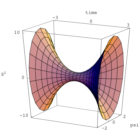
Figure 1: Bounce between two four-dimensional asymptotically de Sitter spacetimes; $\nu=2/3$ and $\mu=0$.

Next, we turn to the case $m=1$. After scaling the metric, we obtain

$$ds^{2}=-\frac{(1+t^{2})^{n}}{\tilde{P}(t)}\,dt^{2}+\frac{c^{2}\,\tilde{P}(t)}{(1+t^{2})^{n}}\,(d\psi-2A)^{2}+c\,(1+t^{2})\,d\Sigma_{2n}^{2}+P_{0}^{-1}\,t^{2}\,d\phi^{2}\,,$$ (2.12)

$$\tilde{P}(t)=\frac{\Lambda}{2(n+1)}\,[(1+t^{2})^{n+1}-1]+\mu\,.$$ (2.13)

For $\mu>0$, the function $P$ is positive-definite and hence the metric describes a bounce between two asymptotic dS_2n+3 spacetimes at $t\rightarrow\pm\infty$. When $\mu=0$, the function $\tilde{P}(t)$ has a second-order zero at $t=0$. In this case, the metric interpolates between dS${}_{3}\times\Sigma_{2n}$ at $t=0$ to dS_2n+3 in the infinite future. For $\mu<0$, $\tilde{P}$ can be negative and there are regions with closed timelike curves.

Finally, we consider the case of $m=0$. Let us define the function $Q(t)$, given by $Q(t)=\tilde{P}(t,\mu=0)$. The requirement that $\tilde{P}(t)$ is positive-definite implies that $Q(t)$ must also be positive-definite. The function $Q(t)$ is non-negative provided that $\nu_{0}\leq\nu\leq 1$, where $\nu_{0}$ is the only positive root of the polynomial equation $Q(\sqrt{{\textstyle{\frac{\scriptstyle 1}{\scriptstyle\nu_{0}}}}-1})=0$. For example, for $n=1$, we have $\nu_{0}={\textstyle{\frac{\scriptstyle 1}{\scriptstyle 4}}}$; for $n=2$, we have $\nu_{0}=(2+\sqrt{10})/12=0.43019$; for $n=3$, we have $\nu_{0}=0.543067$; for $n=4$, we have $\nu_{0}=0.619223$. It is clear that $\nu_{0}$ approaches 1 as $n$ approaches infinity.

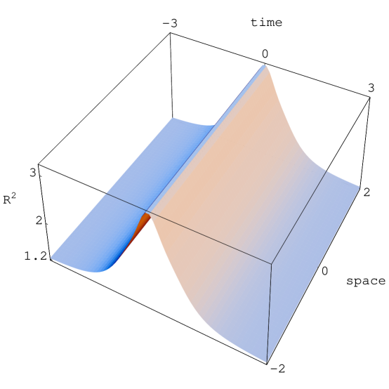
Figure 2: $R^{mnpq}R_{mnpq}$ corresponding to the de Sitter bounce in Figure 1.

Having determined the range of $\nu$ such that $Q(t)$ is non-negative, we can ask what is the range of $\mu$ so $\tilde{P}(t)$ is also non-negative. We find that we need $|\mu|\leq\mu_{0}$, where $\mu_{0}=\Lambda\,Q(t_{0})/t_{0}$ and $t_{0}=\sqrt{{\textstyle{\frac{\scriptstyle 1}{\scriptstyle\nu}}}-1}$. Thus, for $\nu_{0}<\nu<1$ and $|\mu|<\mu_{0}$, the function $\tilde{P}(t)$ is positive-definite and the metric describes a bounce between two asymptotically de Sitter spacetimes. In Figure 1, we plot the radii of the $S^{2}$ and fibre bundle direction $\psi$ as a function of time for the four-dimensional ($n=1$ and $m=0$) de Sitter bounce. We have taken the parameter values $\nu=2/3$, $\mu=0$ and, in the Figure, have chosen the convention that time lies along a horizontal axis. The important property to note is that the radii decrease towards the middle of the bounce but never completely vanish. This corresponds to $R^{mnpq}\,R_{mnpq}$ being well-behaved, as shown in Figure 2. It approaches a finite maximum value in the middle of the bounce and then asymptotes to a lower but positive value corresponding to the asymptotic de Sitter phases.

For $\nu=1$ or $\nu=\nu_{0}$, with $\mu=0$, the function $\tilde{P}(t)$ has a second-order zero at $t_{0}=1$ or $t_{0}=\sqrt{{\textstyle{\frac{\scriptstyle 1}{\scriptstyle\nu_{0}}}}-1}$, respectively and so the solution is dS${}_{2}\times\Sigma_{2n}$ at $t_{0}$. The solution flows from dS${}_{2}\times\Sigma_{2n}$ at time $t_{0}$ to dS_2n+2 in the infinite future. If either $\mu$ or $\nu$ lie outside the range detailed above, then although the solution is free from curvature singularities, the solution contains regions with closed timelike curves. We illustrate this in Figure 3 for the four-dimensional de Sitter bounce for the case of $\nu=1/8$ and $\mu=0$. Again, time runs along the horizontal axis going from left to right. The axis coming out of the page is the radius of the $S^{2}$ as a function of time, which never vanishes. The radius of the fibred direction $\psi$ is plotted along the vertical direction and we have oriented the plot to illustrate that this radius does vanish at four different points, corresponding to Cauchy horizons separating dynamical and stationary regions. There is a time-dependent region in the middle of the bounce, followed and preceded by stationary regions containing closed timelike curves. These, in turn, are followed and preceded by time-dependent regions which asymptote to de Sitter spacetime.

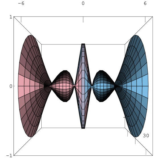
Figure 3: Bounce between two four-dimensional asymptotically de Sitter spacetimes with stationary regions containing closed timelike curves; $\nu=1/8$ and $\mu=0$.

The time-dependent solutions discussed in this section can be regarded as non-singular supergravity S-branes in the presence of a positive cosmological constant. As we shall see, solutions in four and five dimensions can be lifted to supergravity S-brane configurations in eleven and ten dimensions, respectively.

3 $D=4$ charged de Sitter bounce

3.1 General solution

For the case of four dimensions, we can add electric and magnetic charges to the previous de Sitter bounce solution and lift this to eleven dimensions. We take as our starting point a particular case of the Petrov type D solution [48, 50] which corresponds to an AdS Reissner-Nördstrom Taub-NUT solution. This solution is given by

$$ds_{4}^{2} = -\frac{P(r)}{r^{2}+N^{2}}\,(dt-2N\,\cos\phi_{1}\,d\phi_{2})^{2}+\frac{r^{2}+N^{2}}{P(r)}\,dr^{2}+(r^{2}+N^{2})\,d\Omega_{2}^{2}\,,$$

$$A_{{\scriptscriptstyle(1)}} = \frac{q\,r-N\,p}{r^{2}+N^{2}}\,dt-\frac{p(r^{2}-N^{2})+2N\,q\,r}{r^{2}+N^{2}}\,\cos\phi_{1}\,d\phi_{2}\,,$$ (3.1)

$$P(r)=g^{2}(r^{2}+N^{2})^{2}+(1+4g^{2}\,N^{2})(r^{2}-N^{2})-2M\,r+q^{2}+p^{2}\,,$$ (3.2)

and $d\Omega_{2}^{2}=d\phi_{1}^{2}+\sin^{2}\phi_{1}\,d\phi_{2}^{2}$. The constant $N$ is the Taub-NUT parameter, $g$ is the cosmological parameter, and $q$ and $p$ are the electric and magnetic charges. Taking the sign of the cosmological constant to be positive (which amounts to analytically continuing $g\rightarrow{\rm i}\,g$) and relabeling $t\rightarrow\psi$ and $r\rightarrow t$ yields

$$ds_{4}^{2} = \frac{{\tilde{P}}(t)}{t^{2}+N^{2}}\,(d\psi-2N\,\cos\phi_{1}\,d\phi_{2})^{2}-\frac{t^{2}+N^{2}}{{\tilde{P}}(t)}\,dt^{2}+(t^{2}+N^{2})\,d\Omega_{2}^{2}\,,$$

$$A_{{\scriptscriptstyle(1)}} = \frac{q\,t-N\,p}{t^{2}+N^{2}}\,d\psi-\frac{p(t^{2}-N^{2})+2N\,q\,t}{t^{2}+N^{2}}\,\cos\phi_{1}\,d\phi_{2}\,,$$ (3.3)

$${\tilde{P}}(t)=g^{2}(t^{2}+N^{2})^{2}+(1-4g^{2}\,N^{2})(N^{2}-t^{2})+2M\,t-(q^{2}+p^{2})\,.$$ (3.4)

In order to study the properties of this solution, it is worthwhile to calculate the Riemann-squared of the metric which is

$$R_{\mu\nu\rho\sigma}\,R^{\mu\nu\rho\sigma}=24g^{4}+\frac{8}{(t^{2}+N^{2})^{6}}\Bigl{\{}6N^{2}(4g^{2}\,N^{2}-1)(N^{2}-t^{2})(N^{4}-14N^{2}t^{2}+t^{4})$$

$$\ -6M^{2}(N^{2}-t^{2})(N^{4}-14N^{2}t^{2}+t^{4})$$

$$\ -24M\,N^{2}(4g^{2}N^{2}-1)(N^{2}-3t^{2})(3N^{2}-t^{2})\,t$$

$$\ +(p^{2}+q^{2})^{2}(7N^{4}-34N^{2}\,t^{2}+7t^{4})$$ (3.5)

$$\ +12(p^{2}+q^{2})[N^{2}(4g^{2}N^{2}-1)(N^{4}-10N^{2}t^{2}+5t^{4})-M(5N^{4}-10N^{2}t^{2}+t^{4})t]\Bigr{\}}\,.$$

The solution is free of curvature singularities for the entire coordinate range $-\infty<t<+\infty$. In the asymptotic regions $t\rightarrow\pm\infty$, the geometry asymptotes to dS₄. In order for the solution not to have stationary regions with closed timelike curves, it is necessary for the function ${\tilde{P}}(t)$ to be non-negative everywhere.

The quartic function $\tilde{P}(t)$ has either one or two minima. If all the minima are positive, this will ensure that ${\tilde{P}}(t)$ is non-negative. It is convenient to introduce the function $Q(t)=\tilde{P}(t)-(p^{2}+q^{2})$. If the lowest minimum of $Q(t)$, denoted as $Q_{\rm min}$, is non-negative then $\tilde{P}(t)$ can be also non-negative, provided that the electric and magnetic charge parameters $q$ and $p$ satisfy $p^{2}+q^{2}\leq Q_{\rm min}$. Let us assume that the minimum of $Q(t)$ occurs at $t_{0}$, which implies

$$M^{2}=t_{0}^{2}\,(2g^{2}t_{0}^{2}+6g^{2}N^{2}-1)\,,\qquad Q_{\rm min}=(t_{0}^{2}+N^{2})(1-3g^{2}N^{2}-3g^{2}t_{0}^{2})\,.$$ (3.6)

Thus, the condition for $Q_{\rm min}\geq 0$ implies that $g^{2}N^{2}\leq{\textstyle{\frac{\scriptstyle 1}{\scriptstyle 3}}}$ and

$$M^{2}\leq M_{0}^{2}\equiv\frac{(1-3g^{2}N^{2})(12g^{2}N^{2}-1)^{2}}{27g^{2}}\,.$$ (3.7)

In the parameter range ${\textstyle{\frac{\scriptstyle 1}{\scriptstyle 6}}}\leq g^{2}N^{2}\leq{\textstyle{\frac{\scriptstyle 1}{\scriptstyle 3}}}$, there can only be one minimum, and hence (3.7) provides the constraint for the mass parameter $M$. Figure 4 is the plot of the function $Q(t)$ for the case with $g=1$, $N^{2}=1/5$ and $M={\textstyle{\frac{\scriptstyle 1}{\scriptstyle 10}}}<M_{0}$ and in this case there is only one minimum.

Figure 4: Function $Q(t)$ for $g=1$, $N^{2}={\textstyle{\frac{\scriptstyle 1}{\scriptstyle 5}}}$, and $M={\textstyle{\frac{\scriptstyle 1}{\scriptstyle 10}}}$, which has one positive minimum.

When the NUT charge parameter lies in the range ${\textstyle{\frac{\scriptstyle 1}{\scriptstyle 9}}}\leq g^{2}N^{2}<{\textstyle{\frac{\scriptstyle 1}{\scriptstyle 6}}}$, there can be one or two minima depending on the value of $M$. Introduce a parameter

$$\widetilde{M}_{0}^{2}=\frac{2(1-6g^{2}N^{2})^{3}}{27g^{2}}\,,$$ (3.8)

which is less than $M_{0}$ for $g^{2}N^{2}>{\textstyle{\frac{\scriptstyle 1}{\scriptstyle 9}}}$. Thus, for $\widetilde{M}_{0}\leq|M|\leq M_{0}$, the function $Q(t)$ has only one non-negative minimum. For $|M|<\widetilde{M}_{0}$, $Q(t)$ has two non-negative minima.

Finally, if $g^{2}N^{2}<{\textstyle{\frac{\scriptstyle 1}{\scriptstyle 9}}}$, we have $M_{0}<\widetilde{M}_{0}$. $M$ has to be in the range $|M|<M_{0}$, for which there are two positive minima. As an example, we plot the case $g=1$, $N^{2}={\textstyle{\frac{\scriptstyle 1}{\scriptstyle 10}}}$ and $M={\textstyle{\frac{\scriptstyle 1}{\scriptstyle 100}}}$ in Figure 5.

Figure 5: Function $Q(t)$ for $g=1$, $N^{2}={\textstyle{\frac{\scriptstyle 1}{\scriptstyle 10}}}$, and $M={\textstyle{\frac{\scriptstyle 1}{\scriptstyle 100}}}$, which has two positive minima.

In summary, for the parameter range discussed above, $\tilde{P}(t)$ is positive-definite and the metric describes a cosmological bounce between two asymptotic dS₄ when $t\rightarrow\pm\infty$. If we choose the parameters $p$ and $q$ such that the minimum of $\tilde{P}(t)$ is zero at a certain $t_{0}$, then the metric describes dS${}_{2}\times S^{2}$ near the $t_{0}$ region. The solution thus interpolates between dS${}_{2}\times S^{2}$ at the infinite past and dS₄ at the infinite future, with time measured in the co-moving frame. For the parameters lying outside the above range, the function $\tilde{P}(t)$ can become negative and the solution has stationary regions with closed timelike curves.

3.2 BPS solution

Although the above time-dependent solution is not supersymmetric, it arises from a first-order system for the cases in which the corresponding AdS Reissner-Nördstrom Taub-NUT solution is supersymmetric. Thus, the above time-dependent solution might inherit certain properties of the corresponding supersymmetric solution, such as stability [20]. The supersymmetry of the topological AdS Kerr-Newman Taub-NUT solution has been analyzed in [52]. We will focus on the case of the AdS Reissner-Nördstrom Taub-NUT solution, since adding rotation and then analytically continuing $g\rightarrow{\rm i}\,g$ results in closed timelike curves. In addition to the Bogomol’nyi bound of $D=4$ $N=2$ gauged supergravity, given by

$$(M\mp g\,N\,q)^{2}=(1\pm 2g\,p+5g^{2}\,N^{2})(q^{2}+p^{2})-N^{2}\,(1\pm g\,p+4g^{2}\,N^{2})\,,$$ (3.9)

there is also a supersymmetry constraint relating the charges, mass and NUT parameter, given by

$$M\,p=-N\,q\,(1+4g^{2}\,N^{2})\,.$$ (3.10)

Besides two maximally supersymmetric solutions which are both locally AdS, there are solutions which preserve a half and a quarter of the original supersymmetry, for which

$$M_{1/2}=|q\sqrt{1+4g^{2}\,N^{2}}|\,,\qquad p_{1/2}=\pm N\sqrt{1+4g^{2}\,N^{2}}\,,$$ (3.11)

and

$$M_{1/4}=|2g\,N\,q|\,,\qquad p_{1/4}=\frac{1+4g^{2}\,N^{2}}{2g}\,,$$ (3.12)

respectively [52].

When we analytically continue $g\rightarrow{\rm i}\,g$ to a time-dependent solution, we find that only the parameter constraints that originally corresponded to one half preserved supersymmetry lead to a real time-dependent solution. Again, although this does not imply that the time-dependent solution is supersymmetric, it might imply that it is stable. After the analytical continuation, the physical set of parameter constraints is

$$M_{1/2}=|q\sqrt{1-4g^{2}\,N^{2}}|\,,\qquad p_{1/2}=\pm N\sqrt{1-4g^{2}\,N^{2}}\,,$$ (3.13)

In order for the time-dependent solution to obey the above constraints and be free of singularities and closed timelike curves, we require that

$$0<g^{2}\,N^{2}\leq\frac{1}{3}\,,\qquad|M_{1/2}|\leq M_{0}\,,\qquad q^{2}+p_{1/2}^{2}\leq Q_{{\rm min}}\,.$$ (3.14)

For example, for the single-minimum de Sitter bounce solution plotted in Figure 4, all of the above conditions are satisfied for

$$g=1\,,\qquad N=\frac{1}{\sqrt{5}}\,,\qquad M=\frac{1}{10}\,,\qquad q=\frac{1}{2\sqrt{5}}\,,\qquad p=\frac{1}{5\sqrt{5}}\,.$$ (3.15)

On the other hand, the two-minimum de Sitter bounce solution plotted in Figure 5 does not satisfy all of the above constraints.

If the above constraints are to be satisfied, then one can write

$${\tilde{P}}(t)=g^{2}\,t^{4}+(6g^{2}\,N^{2}-1)t^{2}+2q\sqrt{1-4g^{2}\,N^{2}}t+g^{2}\,N^{4}-q^{2}\,.$$ (3.16)

In order to have a real solution, we must have $g\,N\leq 1/2$. The analysis for the requirement that $\tilde{P}(t)$ be non-negative is analogous to that of the more general non-BPS solution that we discussed earlier. Whether the function $\tilde{P}(t)$ has one or two minima depends on the parameters $q$ and $N$. Suppose that the minimum $P_{\rm min}$ occurs at $t_{0}$. Then we have

$$q^{2}=\frac{(8g^{2}N^{2}-1)^{2}}{16g^{2}}\,,\qquad\tilde{P}_{\rm min}=\frac{g^{2}(N^{2}+t^{2})^{2}(1-4g^{2}N^{2}-4g^{2}t_{0}^{2})}{1-4g^{2}N^{2}}\,.$$ (3.17)

Thus, it follows that for $\tilde{P}_{\rm min}\geq 0$, we have $g^{2}N^{2}\leq{\textstyle{\frac{\scriptstyle 1}{\scriptstyle 4}}}$ and

$$q^{2}\leq q_{0}^{2}\equiv\frac{(8g^{2}N^{2}-1)^{2}}{16g^{2}}\,.$$ (3.18)

In the parameter range ${\textstyle{\frac{\scriptstyle 1}{\scriptstyle 6}}}\leq g^{2}N^{2}\leq{\textstyle{\frac{\scriptstyle 1}{\scriptstyle 4}}}$, there can only be one minimum. When the NUT charge parameter lies in the range ${\textstyle{\frac{\scriptstyle 5}{\scriptstyle 36}}}\leq g^{2}\,N^{2}<{\textstyle{\frac{\scriptstyle 1}{\scriptstyle 6}}}$, there can be either one or two minima, depending on the value of $q$. We define $\tilde{q}_{0}^{2}=2(1-6g^{2}N^{2})^{3}/(27g^{2}(1-4g^{2}N^{2}))$, which is smaller than $q_{0}^{2}$ in the above range. The function $\tilde{P}(t)$ has a single non-negative minimum if $\tilde{q}_{0}\leq|q|\leq q_{0}$ and two positive minima instead if $|q|<\tilde{q}_{0}$. For $g^{2}N^{2}<{\textstyle{\frac{\scriptstyle 5}{\scriptstyle 36}}}$, we have $q_{0}<\tilde{q}_{0}$ and $\tilde{P}(t)$ remains non-negative, provided that $|q|\leq q_{0}$.

A second-order zero arises when $P_{\rm min}=0$, which can occur when $|q|=q_{0}$. In this case, the solution interpolates between dS${}_{2}\times S^{2}$ in the infinite past to dS₄ in the infinite future, where time is measured in the comoving frame.

4 De Sitter bounces in M-theory

4.1 Lifting the four-dimensional bounce

We can lift the four-dimensional charged de Sitter bounce to eleven dimensions on a seven-dimensional hyperbolic space [26]. The resulting $SO(4,4)$ gauged solution is given by

$$ds_{11}^{2} = \Delta^{2/3}\,\Big{(}\frac{{\tilde{P}}(t)}{t^{2}+N^{2}}\,(d\psi-2N\,\cos\phi_{1}\,d\phi_{2})^{2}-\frac{t^{2}+N^{2}}{{\tilde{P}}(t)}\,dt^{2}+(t^{2}+N^{2})\,d\Omega_{2}^{2}\Big{)}$$

$$+\frac{1}{\Lambda}\,\Delta^{2/3}\,d\theta^{2}+\frac{1}{4\Lambda}\,\Delta^{-1/3}\,\Big{[}c^{2}\,\Big{(}d{\overline{\Omega}}_{2}^{2}+({\overline{\sigma}}_{3}-\sqrt{\Lambda}A_{{\scriptscriptstyle(1)}})^{2}\Big{)}$$

$$+s^{2}\,\Big{(}{\tilde{\Omega}}_{2}^{2}+({\tilde{\sigma}_{3}}-\sqrt{\Lambda}A_{{\scriptscriptstyle(1)}})^{2}\Big{)}\Big{]}\,,$$

$$F_{{\scriptscriptstyle(4)}} = 2\sqrt{\Lambda}(t^{2}+N^{2})\,(d\psi-2N\,\cos\phi_{1}\,d\phi_{2})\wedge dt\wedge\Omega_{{\scriptscriptstyle(2)}}$$ (4.1)

$$-\frac{1}{4\Lambda}\Big{(}sc\,d\theta\wedge({\overline{\sigma}}_{3}-{\tilde{\sigma}}_{3})-\frac{1}{2}c^{2}\,{\overline{\Omega}}_{{\scriptscriptstyle(2)}}+\frac{1}{2}s^{2}\,{\tilde{\Omega}}_{{\scriptscriptstyle(2)}}\Big{)}\wedge\ast F_{{\scriptscriptstyle(2)}}\,,$$

where $\Delta=\cosh 2\theta$, $c=\cosh\theta$ and $s=\sinh\theta$. $\sigma_{i}$ and $\tilde{\sigma}_{i}$ are $SU(2)$ left-invariant 1-forms satisfying

$$d\sigma_{i}=-{\textstyle{\frac{\scriptstyle 1}{\scriptstyle 2}}}\epsilon_{ijk}\,\sigma_{j}\wedge\sigma_{k}\,,\qquad d\tilde{\sigma}_{i}=-{\textstyle{\frac{\scriptstyle 1}{\scriptstyle 2}}}\epsilon_{ijk}\,\tilde{\sigma}_{j}\wedge\tilde{\sigma}_{k}\,.$$ (4.2)

$F_{{\scriptscriptstyle(2)}}=dA_{{\scriptscriptstyle(1)}}$, where $A_{{\scriptscriptstyle(1)}}$ is given in (3.3). ${\tilde{P}}(t)$ is given in (3.4).

The squashed $S^{3}$ of the four-dimensional bounce and one of the internal $S^{3}$ have strictly positive factors. This ensures that, upon replacing each of these $S^{3}$ by a three-dimensional lens space $S^{3}/Z_{Q}$ and reducing and T-dualizing over the two fibre coordinates, the resulting time-dependent solution of type IIB theory is non-singular.

For vanishing electric and magnetic charges, we can also embed the solution in eleven dimensions as an $SO(5,3)$ gauged solution [54], given by

$$ds_{11}^{2} = \tilde{\Delta}^{2/3}\,(-\frac{1+t^{2}}{\tilde{P}(t)}\,dt^{2}+\frac{\tilde{P}(t)}{1+t^{2}}\,(d\psi-2\tilde{A})^{2}+(1+t^{2})\,d\Omega_{2}^{2})$$

$$+\frac{1}{\Lambda}\,\tilde{\Delta}^{-1/3}\,\Bigl{(}\frac{1}{9}(2\cosh(2\theta)+1)\,d\theta^{2}+\cosh^{2}\theta\,d\Omega_{4}^{2}+\frac{1}{3}\sinh^{2}\theta\,\tilde{\Omega}_{2}^{2}\Bigr{)}\,,$$

$$F_{{\scriptscriptstyle(4)}} = 2\sqrt{\Lambda}\,\epsilon_{{\scriptscriptstyle(4)}}\,.$$ (4.3)

$$\tilde{\Delta}=\frac{1}{3}(5\cosh(2\theta)-2)\,.$$ (4.4)

4.2 Lifting the five-dimensional bounce

Five-dimensional solutions are given by (2.12) and (2.13), for which $m=1$ and $n=1$. These include solutions which smoothly run from dS${}_{3}\times\Sigma_{2}$ to dS₅, as well as bounces between two phases of dS₅. These solutions can be embedded in ten-dimensional type IIB theory as

$$ds_{10}^{2} = \Delta^{1/2}\,\Big{(}-\frac{1+t^{2}}{\tilde{P}(t)}\,dt^{2}+\frac{\tilde{P}(t)}{1+t^{2}}\,(d\psi-2A)^{2}+(1+t^{2})\,d\Omega_{2}^{2}+t^{2}\,d\phi^{2}\Big{)}$$

$$+\frac{1}{\Lambda}\,\Delta^{1/2}\,d\theta^{2}+\frac{1}{\Lambda}\,\Delta^{-1/2}\,(\cosh^{2}\theta\,d\Omega_{2}^{2}+\sinh^{2}\theta\,\tilde{\Omega}_{2}^{2})\,,$$

$$F_{{\scriptscriptstyle(5)}} = 2\sqrt{\Lambda}\,(\epsilon_{{\scriptscriptstyle(5)}}+\ast\epsilon_{{\scriptscriptstyle(5)}})\,,$$ (4.5)

where $\Delta=\cosh 2\theta$ and $\epsilon_{{\scriptscriptstyle(5)}}$ is the volume-form corresponding to the five-dimensional metric. We have set $c$ and $P_{0}$ to unity for simplicity.

As before, we can replace the $S^{3}$ of the five-dimensional metric by $S^{3}/Z_{q}$. The solution can then be Hopf T-dualized and lifted to yield a non-singular time-dependent solution in eleven dimensions.

5 Conclusions

The analytical continuation of recently-found de Sitter instantons leads to asymptotically de Sitter cosmological solutions, which include smooth de Sitter bounces. In four dimensions, we were able to generalize this construction to obtain a de Sitter bounce with electric and magnetic charges, by analytically continuing the AdS Reissner-Nördstrom Taub-NUT solution. Four and five-dimensional de Sitter bounces can be lifted to non-singular time-dependent configurations in eleven-dimensional supergravity and type IIB theory, respectively. These bounces are completely regular in a purely classical gravity setting. They asymptotically approach de Sitter spacetime in both the infinite past and infinite future but deviate from de Sitter during intermediate times, with respect to the comoving time. It is clear that further analytical continuations of these solutions can be performed, which may lead to more non-singular solutions. This will be discussed elsewhere.

These solutions are potentially interesting new backgrounds on which to study dS/CFT-type holography [58] in the case where the conformal symmetry is broken throughout the cosmological evolution and restored at very early and late times. It has been postulated that a cosmological flow corresponds to a renormalization group flow between two conformal fixed points of a three-dimensional Euclidean field theory [60]. However, our cosmological solution which runs from dS${}_{2}\times S^{2}$ to dS₄ corresponds to a flow “across dimensions” from a one-dimensional Euclidean field theory to a three-dimensional Euclidean field theory. The solution can be fine-tuned to expand quickly from the dS${}_{2}\times S^{2}$ fixed-point. In this case, the early-time behavior might not be completely unrealistic. In fact, this fixed-point might leave an observable imprint on the CMB as a contribution to the quadrupole moment. The solution can be fine-tuned to describe an expanding universe whose expansion rate is significantly larger in the past than in the future, providing an inflationary model with no singularity. With regards to the de Sitter bounces, it has been postulated that the Euclidean field theory on only one of the boundaries is physically relevant [58].

It is interesting to study the dampening effects of the cosmological constant in our solutions. For vanishing mass, NUT charge, and electric and magnetic charges, the cosmological bounce reduces to pure de Sitter in global coordinates. As the other parameters are turned on, the effect of the cosmological constant can be reduced. If this dampening effect occurred at late times then this could have some interesting ramifications with regards to the cosmological constant problem. The mass parameter breaks the symmetry of the bounce solution about the central region. Thus, we postulate that the cosmological bounce could be fine-tuned to have a longer period of slow contraction. If this is the case, then the cosmological bounce is a viable alternative to inflation. In particular, during the end of the contracting phase, currently-observed cosmological scales would be well inside the Hubble radius, providing ample time for the observed homogeneity to occur through causal microphysics.

References

- [1]
- [2] G. Veneziano, Phys. Lett. B265 (1991) 287.
- [3]
- [4] M. Gasperini and G. Veneziano, Pre-Big-Bang in string cosmology, Astropart. Phys. 1 (1993) 317, hep-th/9211021.
- [5]
- [6] J. Khoury, B.A. Ovrut, P.J. Steinhardt and N. Turok, The Ekpyrotic universe: colliding branes and the origin of the hot big bang, Phys. Rev. D64 (2001) 123522, hep-th/0103239.
- [7]
- [8] I. Antoniadis, J. Rizos and K. Tamvakis, Singularity-free cosmological solutions of the superstring effective action, Nucl. Phys. B415 (1994) 497, hep-th/9305025.
- [9]
- [10] A. Lukas, B.A. Ovrut and D. Waldram, Cosmological solutions of type II string theory, Phys. Lett. B393 (1997) 65, hep-th/9608195.
- [11]
- [12] H. Lü, S. Mukherji, C.N. Pope and K.W. Xu, Cosmological solutions in string theories, Phys. Rev. D55 (1997) 7926, hep-th/9610107.
- [13]
- [14] A. Lukas, B.A. Ovrut and D. Waldram, String and M-theory cosmological solutions with Ramond forms, Nucl. Phys. B495 (1997) 365, hep-th/9610238.
- [15]
- [16] H. Lü, S. Mukherji and C.N. Pope, From p-branes to cosmology, Int. J. Mod. Phys. A14 (1999) 4121, hep-th/9612224.
- [17]
- [18] M. Gutperle and A. Strominger, Spacelike branes, JHEP 0204 (2002) 018, hep-th/0202210.
- [19]
- [20] K. Behrndt and M. Cvetič, Time-dependent backgrounds from supergravity with gauged non-compact R-symmetry, Class. Quant. Grav. 20 (2003) 4177, hep-th/0303266.
- [21]
- [22] H. Lü and J.F. Vázquez-Poritz, From AdS black holes to supersymmetric flux-branes, hep-th/0307001.
- [23]
- [24] H. Lü and J.F. Vázquez-Poritz, From de Sitter to de Sitter, JCAP 0402 (2004) 004, hep-th/0305250.
- [25]
- [26] H. Lü and J.F. Vázquez-Poritz, Four-dimensional Einstein Yang-Mills de Sitter gravity from eleven dimensions, hep-th/0308104.
- [27]
- [28] H. Lü and J.F. Vázquez-Poritz, Smooth cosmologies from M-theory, hep-th/0401150.
- [29]
- [30] G. Jones, A. Maloney and A. Strominger, Non-singular solutions for S-branes, hep-th/0403050.
- [31]
- [32] J.E. Wang, Twisting S-branes, hep-th/0403094.
- [33]
- [34] G. Tasinato, I. Zavala, C.P. Burgess and F. Quevedo, Regular S-brane backgrounds, JHEP 0404 (2004) 038, hep-th/0403156.
- [35]
- [36] H. Lü and J.F. Vázquez-Poritz, Non-singular twisted S-branes from rotating branes, hep-th/0403248.
- [37]
- [38] I.R. Klebanov and M.J. Strassler, Supergravity and a confining gauge theory: duality cascades and SB-resolution of naked singularities, JHEP 0008 (2000) 052, hep-th/0007191.
- [39]
- [40] S. Perlmutter et al. [Supernova Cosmology Project Collaboration], Measurements of the cosmological parameters and from the first supernovae at , Astrophys. J. 483 (1997) 565, astro-ph/9608192.
- [41]
- [42] A.G. Riess et al. [Supernova Search Team Collaboration], Observational evidence from supernovae for an accelerating universe and a cosmological constant, Astron. J. 116 (1998) 1009, astro-ph/9805201.
- [43]
- [44] H. Lü, D.N. Page and C.N. Pope, New inhomogeneous Einstein metrics on sphere bundles over Einstein-Kähler manifolds, hep-th/0403079.
- [45]
- [46] R. Mann and C. Stelea, Nuttier (A)dS black holes in higher dimensions, hep-th/0312285.
- [47]
- [48] J.F. Plebanski and M. Demianski, Ann. Phys. 98 (1976) 98.
- [49]
- [50] J.F. Plebanski, Ann. Phys. 90 (1975) 196.
- [51]
- [52] N. Alonso-Alberca, P. Meessen and T. Ortin, Supersymmetry of topological Kerr-Newman-Taub-NUT-AdS spacetimes, Class. Quant. Grav. 17 (2000) 2783, hep-th/0003071.
- [53]
- [54] G.W. Gibbons and C.M. Hull, De Sitter space from warped supergravity solutions, hep-th/0111072.
- [55]
- [56] M. Cvetič, H. Lü, C.N. Pope and J.F. Vázquez-Poritz, AdS in warped spacetimes, Phys. Rev. D62 (2000) 122003, hep-th/0005246.
- [57]
- [58] A. Strominger, The dS/CFT crrespondence, JHEP 10 (2001) 034, hep-th/ 0106113.
- [59]
- [60] A. Strominger, Inflation and the dS/CFT correspondence, JHEP 11 (2001) 049, hep-th/0110087.
- [61]
- [62] J. Maldacena and C. Nuñez, Supergravity description of field theories on curved manifolds and a no go theorem, Int. J. Mod. Phys. A16 (2001) 822, hep-th/0007018.
- [63]
- [64] S. Cucu, H. Lü and J.F. Vazquez-Poritz, A supersymmetric and smooth compactification of M-theory to AdS5 Phys. Lett. B568, 261 (2003), hep-th/0303211.
- [65]
- [66] S. Cucu, H. Lü and J.F. Vazquez-Poritz, Interpolating from AdS to AdSD, Nucl. Phys. B677, 181 (2004), hep-th/0304022.
- [67]