Electric/magnetic deformations of $S^{3}$ and $\mathrm{AdS}_{3}$ , and geometric cosets

Abstract:

We analyze asymmetric marginal deformations of $SU(2)_{k}$ and $SL(2,\mathbb{R})_{k}$ wzw models. These appear in heterotic string backgrounds with non-vanishing Neveu–Schwarz three-forms plus electric or magnetic fields, depending on whether the deformation is elliptic, hyperbolic or parabolic. Asymmetric deformations create new families of exact string vacua. The geometries which are generated in this way, deformed $S^{3}$ or $\mathrm{AdS}_{3}$, include in particular geometric cosets such as $S^{2}$, $\mathrm{AdS}_{2}$ or $H_{2}$. Hence, the latter are consistent, exact conformal sigma models, with electric or magnetic backgrounds. We discuss various geometric and symmetry properties of the deformations at hand as well as their spectra and partition functions, with special attention to the supersymmetric $\mathrm{AdS}_{2}\times S^{2}$ background. We also comment on potential holographic applications.

1 Introduction

Near-horizon geometries of NS5-branes [1, 2, 3], NS5/F1 or S-dual versions of those [4, 5] have been thoroughly analyzed over the past years. These involve $\mathrm{AdS}_{3}$ or $S^{3}$ spaces and turn out to be exact string backgrounds, tractable beyond the supergravity approximation. They offer a unique setting in which to analyze AdS/cft correspondence, black-hole physics, little-string theory…

An important, and not yet unravelled aspect of such configurations is the investigation of their moduli space. String propagation in the above backgrounds is described in terms of some exact two-dimensional conformal field theory. Hence, marginal deformations of the latter provide the appropriate tool for exploring the moduli of the corresponding string vacua.

A well-known class of marginal deformations for wzw models are those driven by left-right current bilinears [6, 7]: $\int{\,\mathrm{d}}^{2}z\ J\bar{J}$. These can be “symmetric” in the sense that both $J$ and $\bar{J}$ are generators of the affine algebra of the wzw model. However, asymmetric deformations can also be considered, where either $J$ or $\bar{J}$ correspond to some other $U(1)$, living outside of the chiral algebra of the wzw model. These deformations describe the response of the system to a finite (chromo) electric or magnetic background field and since these deformations are exactly marginal, the gravitational back-reaction is properly taken into account at any magnitude of the external field [8, 9].

The purpose of this note is to report on the asymmetric deformations of the $SL(2,\mathbb{R})_{k}$ heterotic string background. Since $SL(2,\mathbb{R})$ has time-like, null and space-like generators, three distinct asymmetric deformations are possible, corresponding respectively to magnetic, electromagnetic and electric field backgrounds. The former case has been recently analyzed from this perspective [10] and the corresponding deformation was shown to include Gödel space–time, which is therefore promoted to an exact string background (despite the caveats of closed time-like curves). The latter case, on the other hand, corresponds to a new deformation, which connects $\mathrm{AdS}_{3}$ with $\mathbb{R}\times\mathrm{AdS}_{2}$.

This observation is far reaching: while symmetric deformations usually connect wzw models to some $U(1)$-gauged version of them [11], asymmetric deformations turn out to connect the original theory to some geometric coset, with electric or magnetic background fields. This holds for the $SU(2)_{k}$, where the limiting magnetic deformation has $\mathbb{R}\times S^{2}$ geometry, and can be generalized to any wzw model: geometric cosets with electric or magnetic background fields provide thus exact string vacua. Here we focus on the $S^{2}$ and AdS₂ examples, previously discussed as heterotic coset constructions in [12] (see also [13]). Moreover, they both enter in the near-horizon geometry of the four-dimensional Reissner–Nordström extremal black hole, AdS${}_{2}\times S^{2}$, which is here shown to be an exact string vacuum. We also show how $H_{2}$ appears as an exact cft, although this background is of limited interest for string theory because of lack of unitarity.

The paper is organized as follows. First we review the magnetic deformation of $S^{3}$, appearing in the framework of the $SU(2)_{k}$ wzw model. The appearance of the two-sphere plus magnetic field as exact string background is described in Sec. 2, where we also determine the corresponding partition function. The $\mathrm{AdS}_{3}$ case is analyzed in Sec. 3, where its asymmetric deformations are described in detail from geometrical and two-dimensional-cft points of view. We also investigate their spectra. Limiting deformations are discussed in Sec. 4. There, we show how to reach the $\mathrm{AdS}_{2}=SL(2,\mathbb{R})/U(1)$ geometric coset with electric field. These backgrounds are consistent and exact string vacua.

The $H_{2}$ geometric coset of AdS₃ is also shown to appear on the line of magnetic deformation, with imaginary magnetic field though. The near-horizon geometry of the four-dimensional Reissner–Nordström extremal black hole is further discussed in Sec. 5. Section 6 contains a collection of final comments, where we sort various geometries that should be investigated in order to get a comprehensive picture of the general AdS₃ landscape, and its connection to other three-dimensional geometries. Four appendices provide some complementary/technical support. Appendix A sets the general framework for geometric deformations of a metric, designed to keep part of its original isometry. Appendices B and C contain material about $SU(2)$ and $SL(2,\mathbb{R})$ groups manifolds. A reminder of low-energy field equations for the bosonic degrees of freedom of heterotic string is given in App. D.

2 Magnetic deformation of $S^{3}$

$SU(2)_{k}$ wzw model magnetic deformations were analyzed in [8, 9], for both type II and heterotic string backgrounds. For concreteness, we will concentrate here on the latter case. In contrast to what happens in flat space–time, these deformations are truly marginal in the background of a three-sphere plus ns flux, and preserve $N=(1,0)$ world-sheet supersymmetry.

Consider heterotic string on $\mathbb{R}^{1,3}\times S^{3}\times T^{4}$. The theory is critical provided we have a linear dilaton living on the $\mathbb{R}^{1,3}$, with background charge $Q=1/\sqrt{k+2}$, where $k$ is the level of the bosonic $SU(2)_{\rm L}\times SU(2)_{\rm R}$ affine algebra. The target-space geometry is the near-horizon limit of the solitonic NS5-brane [1, 2, 3].

The two-dimensional $N=(1,0)$ world-sheet action corresponding to the $S^{3}$ factor is

$$S_{SU(2)_{k}}=\frac{1}{2\pi}\int{\rm d}^{2}z\left\{\frac{k}{4}\left(\,\partial\alpha\,\bar{\partial}\alpha+\,\partial\beta\,\bar{\partial}\beta+\,\partial\gamma\,\bar{\partial}\gamma+2\cos\beta\,\,\partial\alpha\,\bar{\partial}\gamma\right)+\sum_{a=1}^{3}\psi^{a}\,\bar{\partial}\psi^{a}\right\},$$ (1)

where $\psi^{a}$ are the left-moving free fermions, superpartners of the bosonic $SU(2)_{k}$ currents, and $(\alpha,\beta,\gamma)$ are the usual Euler angles parameterizing the $SU(2)$ group manifold (see App. B for a reminder). In this parameterization, the chiral currents of the Cartan subalgebra read:

$$J^{3}=k\left(\,\partial\gamma+\cos\beta\,\partial\alpha\right)\ ,\ \ \bar{J}^{3}=k\left(\,\bar{\partial}\alpha+\cos\beta\,\,\bar{\partial}\gamma\right)$$ (2)

(Tab. 1) with the following short-distance expansion:

$$J^{3}(z)J^{3}(0)={k\over 2z^{2}}+{\rm reg.}$$ (3)

and similarly for the right-moving one. The left-moving fermions transform in the adjoint of $SU(2)$. There are no right-moving superpartners but a right-moving current algebra with total central charge $c=16$ (realized e.g. in terms of right-moving free fermions). The currents of the latter are normalized so that the Cartan generators $\bar{J}^{i}_{G}$ of the group factor $G$ satisfy the following short-distance expansion:

$$\bar{J}^{i}_{G}(z)\bar{J}^{j}_{G}(0)={k_{G}h^{ij}\over 2\bar{z}^{2}}+{\rm reg.}\ ,\ \ i,j=1,\ldots,{\rm rank}(G)$$ (4)

with $h^{ij}{\vphantom{k}}=f^{ik}_{\hphantom{ik}\ell}\,f^{\ell j}_{\hphantom{ij}k}\big{/}g^{\ast}$, $f^{ij}_{\hphantom{ik}k}$ and $g^{\ast}$ being the structure constants and dual Coxeter number of the group $G$.

The background metric and NS two-form are read off directly from (1):

$${\,\mathrm{d}}s^{2} =\frac{k}{4}\left[{\,\mathrm{d}}\beta^{2}+\sin^{2}\beta{\,\mathrm{d}}\alpha^{2}+\left({\,\mathrm{d}}\gamma+\cos\beta{\,\mathrm{d}}\alpha\right)^{2}\right],$$ (5)

$$B =\frac{k}{4}\cos\beta{\,\mathrm{d}}\alpha\land{\,\mathrm{d}}\gamma.$$ (6)

They describe a three-sphere of radius $L=\sqrt{k}$ and a ns three-form whose field strength is ${\,\mathrm{d}}B=\frac{2}{\sqrt{k}}\,\omega_{[3]}$ ($\omega_{[3]}$ stands for the volume form given in Eq. (96)).

A comment is in order here. In general, the background fields $G_{ab}$, $B_{ab}$, …receive quantum corrections due to two-dimensional renormalization effects controlled by $\alpha^{\prime}$ (here set equal to one). This holds even when the world-sheet theory is exact. Conformal invariance requires indeed the background fields to solve Eqs. (130) that receive higher-order $\alpha^{\prime}$ corrections. The case of wzw models is peculiar in the sense that the underlying symmetry protects $G_{ab}$ and $B_{ab}$ from most corrections; these eventually boil down to the substitution $k\to k+2$ in Eqs. (5) and (6), see e.g. [14].

Notice finally that the $SU(2)_{k}$ plus linear dilaton background introduces a mass gap with respect to flat space: $\mu^{2}={1/(k+2)}$. This plays the role of infra-red regulator, consistent with all string requirements including worldsheet supersymmetry.

2.1 Squashing the three-sphere

We now turn to the issue of conformal deformations. As already advertised, we will not consider left-right symmetric ones, which are purely gravitational. Instead, we will switch the following $N=(1,0)$ world-sheet supersymmetry compatible perturbation on

$$\delta S_{\rm magnetic}=\frac{\sqrt{kk_{G}}H}{2\pi}\int{\rm d}^{2}z\left(J^{3}+\imath\psi^{1}\psi^{2}\right)\bar{J}_{G};$$ (7)

$\bar{J}_{G}$ being any Cartan current of the group factor $G$.

Although one may easily show the integrability of this marginal perturbation out of general arguments (see e.g. [6]) it is instructive to pause and write an explicit proof. If we limit ourselves to the bosonic sector, we can bosonize the $\bar{J}_{G}$ current as $\bar{J}_{G}=\imath\bar{\partial}\varphi$ and interpret $\varphi\left(z,\bar{z}\right)$ as an internal degree of freedom (see App. D for a more precise discussion). Incorporating the kinetic term for the $\varphi$ field, the deformed action reads:

$$S=S_{SU\left(2\right)_{k}}\left(\alpha,\beta,\gamma\right)+\delta S_{\text{magnetic}}+\frac{k_{G}}{4\pi}\int{\,\mathrm{d}}^{2}z\,\partial\varphi\bar{\partial}\varphi,$$ (8)

where $S_{SU\left(2\right)_{k}}$ (Eq. (1)) now contains the bosonic degrees of freedom only. The terms in previous expression can be recollected so to give:

$$S=S_{SU\left(2\right)_{k}}\left(\alpha,\beta,\gamma+2\sqrt{\frac{k_{G}}{k}}H\varphi\right)+\frac{k_{G}\left(1-2H^{2}\right)}{4\pi}\int{\,\mathrm{d}}^{2}z\,\partial\varphi\bar{\partial}\varphi,$$ (9)

which is manifestly an exact cft. As a corollary, we observe that in the present setting, $\mathcal{O}\left(\alpha^{\prime}\right)$ solutions of Eqs. (130) are automatically promoted to all-order exact solutions by simply shifting $k\to k+2$, just like for an “ordinary” wzw model.

The effect of the deformation at hand is to turn a (chromo)magnetic field on along some Cartan direction inside $G$, which in turn induces a gravitational back-reaction on the metric and the three-form antisymmetric tensor. Following the previous discussion and App. D (i.e. by using Kaluza–Klein reduction), it is straightforward to read off the space–time backgrounds from (1) and (7). We obtain:

$${\,\mathrm{d}}s^{2}=\frac{k}{4}\left[{\,\mathrm{d}}\beta^{2}+\sin^{2}\beta{\,\mathrm{d}}\alpha^{2}+\left(1-2H^{2}\right)\left({\,\mathrm{d}}\gamma+\cos\beta{\,\mathrm{d}}\alpha\right)^{2}\right]$$ (10)

and

$$A=\sqrt{\frac{2k}{k_{G}}}H\left({\,\mathrm{d}}\gamma+\cos\beta{\,\mathrm{d}}\alpha\right)$$ (11)

for the metric and gauge field, whereas neither the $B$-field nor the dilaton are altered. The three-form field strength is however modified owing to the presence of the gauge field (see Eqs. (130)):

$$H_{[3]}={\,\mathrm{d}}B-\frac{k_{G}}{4}A\land{\,\mathrm{d}}A=\frac{k}{4}\left(1-2H^{2}\right)\sin\beta{\,\mathrm{d}}\alpha\land{\,\mathrm{d}}\beta\land{\,\mathrm{d}}\gamma$$ (12)

(the non-abelian structure of the gauge field plays no role since the non-vanishing components are in the Cartan subalgebra).

The deformed geometry (10) is a squashed three-sphere: its volume decreases with respect to the original $S^{3}$ while its curvature increases. These properties are captured in the expressions of the volume form and Ricci scalar:

$$\omega_{[3]}=\left(\frac{k}{4}\right)^{3/2}\sqrt{\left|1-2H^{2}\right|}\,\sin\beta{\,\mathrm{d}}\alpha\land{\,\mathrm{d}}\beta\land{\,\mathrm{d}}\gamma,$$ (13)

$$R=\frac{2}{k}(3+2H^{2}).$$ (14)

The latter is constant and the background under consideration has $U(1)\times SU(2)$ isometry generated by the Killing vectors $\mathinner{\{{L_{3},R_{1},R_{2},R_{3}}\}}$ whose explicit expression is reported in App. B, Tab. 1.

This situation should be compared to the symmetric deformation generated by the the marginal operator $\left(J^{3}+i\psi^{1}\psi^{2}\right)\bar{J}^{3}$. This is purely gravitational and alters the metric, the $B$-field and the dilaton [11]. The isometry is in that case broken to $U(1)\times U(1)$ and the curvature is not constant.

At this point one might wonder to what extent the constant curvature of the asymmetric deformation is due to the large (almost maximal) residual isometry $U(1)\times SU(2)$. This question is answered in App. A, where it is shown, in a general framework, that the isometry requirement is not stringent enough to substantially reduce the moduli space of deformations. In particular, the resulting curvature is in general not constant.

In the case under consideration, however, the geometric deformation is driven by an integrable marginal perturbation of the sigma-model. Combined with the left-over isometry, this requirement leads to the above geometry with constant curvature, Eq. (14). From a purely geometrical point of view (i.e. ignoring the CFT origin), such a deformation joins the subclass of one-parameter families described in App. A, obtained by demanding stability i.e. integrability on top of the symmetry.

Notice finally that the $U(1)\times SU(2)$ isometry originates from an affine symmetry at the level of the sigma-model. The asymmetric marginal deformation under consideration breaks the original affine $SU(2)_{\rm L}$ down to $U(1)_{\rm L}$, while it keeps the affine $SU(2)_{\rm R}$ unbroken.

It is worthwhile stressing that this asymmetric and the previously quoted symmetric deformations of the three-sphere background are mutually compatible and can be performed simultaneously [8, 9].

All the above discussion about integrability, geometry and isometries of the $SU(2)_{k}$ magnetic perturbation is valid for the various asymmetric deformations of $SL(2,\mathbb{R})$ that will be analysed in Sec. 3.

2.2 Critical magnetic field and the geometric coset

It was made clear in [11] that the symmetric deformation of $SU(2)_{k}$ wzw is a well-defined theory for any value of the deformation parameter. For an infinite deformation, the sigma-model becomes a gauged wzw model $SU(2)_{k}/U(1)$ (bell geometry) times a decoupled boson. In some sense, the two $U(1)$ isometries present on the deformation line act, for extreme deformation, on two disconnected spaces: the bell and the real line.

As already stressed, the magnetic deformation of $SU(2)_{k}$ preserves a larger symmetry, namely a $U(1)\times SU(2)$, and has constant curvature. We are in the framework discussed in App. A, Eqs. (85) and (87) with $h=2H^{2}$. This deformation has an end-point where the space is expected to factorize into a line with $U(1)$ isometry and a two-dimensional constant-curvature space with $SU(2)$ isometry, which can only be a two-sphere.

These statements can be made more precise by considering the background (10). The deformation parameter $H^{2}$ is clearly bounded: $H^{2}\leqslant 1/2$ (the boundary $H_{\text{max}}^{2}=1/2$ of the moduli space is reminiscent of the $\mathrm{Im}\left(U\right)\to\infty$ limit in a two-dimensional toroidal compactification). In general, a three sphere can be seen as an $S^{1}$-Hopf fibration over a base $S^{2}$. It is clear from expressions (10) and (13) that the effect of the magnetic field consists in changing the radius of the fiber. At $H^{2}=H_{\text{max}}^{2}$, this radius vanishes. The corresponding dimension decompactifies, and factorizes from the three-dimensional geometry:

$$S^{3}\xrightarrow[H^{2}\to H_{\text{max}}^{2}]{}\mathbb{R}\times S^{2},$$ (15)

where $S^{2}$ is the geometric coset $SU(2)/U(1)$. The $M_{H}\to SU(2)/U(1)$ fibration trivializes in this limit. This can be made more transparent by introducing a new coordinate:

$$y=\sqrt{{k\over 2}\left({1\over 2}-H^{2}\right)}\,\gamma.$$ (16)

The metric and volume form now read:

$${\,\mathrm{d}}s^{2}=\frac{k}{4}\left[{\,\mathrm{d}}\beta^{2}+\sin^{2}\beta{\,\mathrm{d}}\alpha^{2}\right]+{\,\mathrm{d}}y^{2}+2\sqrt{{k\over 2}\left({1\over 2}-H^{2}\right)}\,\cos\beta\,{\,\mathrm{d}}\alpha{\,\mathrm{d}}y+{k\over 2}\left({1\over 2}-H^{2}\right)\cos^{2}\beta{\,\mathrm{d}}\alpha^{2}$$ (17)

and

$$\omega_{[3]}=\frac{k}{4}\,\sin\beta{\,\mathrm{d}}\alpha\land{\,\mathrm{d}}\beta\land{\,\mathrm{d}}y.$$ (18)

For $H^{2}$ close to $H^{2}_{\text{max}}$, the $y$-direction factorizes

$${\,\mathrm{d}}s^{2}\xrightarrow[H^{2}\to H^{2}_{\text{max}}]{}{\,\mathrm{d}}y^{2}+\frac{k}{4}\left[{\,\mathrm{d}}\beta^{2}+\sin^{2}\beta{\,\mathrm{d}}\alpha^{2}\right],$$ (19)

while the curvature ($R\to 8/k$) is entirely supported by the remaining two-sphere of radius $\sqrt{k/4}$. The other background fields read:

$$F =\sqrt{\frac{2k}{k_{G}}}H\sin\beta{\,\mathrm{d}}\alpha\land{\,\mathrm{d}}\beta\xrightarrow[H^{2}\to H^{2}_{\text{max}}]{}\sqrt{\frac{k}{k_{G}}}\sin\beta{\,\mathrm{d}}\alpha\land{\,\mathrm{d}}\beta,$$ (20)

$$H_{[3]} =\sqrt{{k\over 2}\left({1\over 2}-H^{2}\right)}\sin\beta{\,\mathrm{d}}\alpha\land{\,\mathrm{d}}\beta\land{\,\mathrm{d}}y\xrightarrow[H^{2}\to H^{2}_{\text{max}}]{}0.$$ (21)

The above analysis deserves several comments. Our starting point was a marginal deformation of the $SU(2)_{k}$ wzw model embedded in heterotic strings and induced by a space–time (chromo)magnetic field. Our observation is here that the corresponding moduli space has a boundary, where the background is $\mathbb{R}\times S^{2}$, with finite magnetic field and no three-form NS background. Being a marginal deformation, this background is exact, showing thereby that the geometric coset is as good as a gauged wzw model background. The latter appears similarly as the end-point of a purely gravitational deformation; it carries neither magnetic field nor $H_{[3]}$, but has a non-trivial dilaton.

Notice also that it was observed in the past that $S^{2}$ could provide part of a string vacuum in the presence of rr fluxes [15], but as usual when dealing with rr fluxes, no exact conformal field theory description is available.

The procedure we have developed so far for obtaining the two-sphere as an exact background in the presence of a magnetic field is easily generalizable to other geometric cosets of compact or non-compact groups. We will focus on the latter case is Sec. 3, and analyze the electric/magnetic deformations of AdS₃.

Our last comment concerns the quantization of the magnetic flux. Indeed the two-sphere appears naturally as a factor of magnetic monopoles backgrounds [16]. At the limiting value of the deformation, the flux of the gauge field through the two-sphere is given by:

$$\mathcal{Q}=\int_{S^{2}}F=\sqrt{\frac{k}{k_{G}}}\int_{S^{2}}\hat{\omega}_{2}=\sqrt{\frac{k}{k_{G}}}4\pi,$$ (22)

where $\hat{\omega}_{2}$ stands for the volume form of a unit-radius two-sphere. Therefore, a quantization of the magnetic charge is only compatible with levels of the affine algebras such that:

$$\frac{k}{k_{G}}=p^{2}\ ,\ \ p\in\mathbb{Z}.$$ (23)

Actually, it was shown in [12] that the model corresponding to the critical magnetic field can be obtained directly with the following asymmetric gauged wzw model:

$$\frac{SU(2)_{k}\times U(1)_{k_{G}}}{U(1)},$$ (24)

where the left gauging lies in the $SU(2)_{k}$ wzw model and the right gauging in the $U(1)_{k_{G}}$ of the gauge sector. The cancellation of the anomalies of the coset dictates a condition on the level of $SU(2)_{k}$ similar to (23).

2.3 Character formulas and modular invariance

We will here construct the contribution of the squashed three-sphere to the partition function. This contribution is modular-covariant, and combines with the remaining degrees of freedom into a modular-invariant result. Our computation will also include the $S^{2}$ limiting geometry. We will consider the case $k_{G}=2$, i.e. a $U(1)$ algebra generated by one right-moving complex fermion. We begin with the following combination of $SU(2)_{k}$ supersymmetric characters and fermions from the gauge sector:

$$Z{a;h\atopwithdelims[ ]b;g}=\sum_{j,\bar{\jmath}=0}^{(k-2)/2}M^{j\bar{\jmath}}\ \chi^{j}\ \frac{\vartheta{a\atopwithdelims[ ]b}}{\eta}\ \bar{\chi}^{\bar{\jmath}}\ \frac{\bar{\vartheta}{h\atopwithdelims[ ]g}}{\bar{\eta}}.$$ (25)

where the $\chi^{j}$’s are the characters of bosonic $SU(2)_{k-2}$, $(a,b)$ are the $\mathbb{Z}_{2}$ boundary conditions for the left-moving fermions and $(h,g)$ those of the right-moving – gauge-sector – ones. We can choose any matrix $M^{j\bar{\jmath}}$ compatible with modular invariance of $SU(2)_{k-2}$. Furthermore, the supersymmetric $SU(2)_{k}$ characters can be decomposed in terms of those of the $N=2$ minimal models:

$$\chi^{j}(\tau)\ \vartheta{a\atopwithdelims[ ]b}(\tau,\nu)=\sum_{m\in\mathbb{Z}_{2k}}\mathcal{C}^{j}_{m}{a\atopwithdelims[ ]b}\Theta_{m,k}\left(\tau,-\frac{2\nu}{k}\right),$$ (26)

where the $N=2$ minimal-model characters, determined implicitly by this decomposition, are given in [17, 18, 19, 20].

Our aim is to implement the magnetic deformation in this formalism. The deformation acts as a boost on the left-lattice contribution of the Cartan current of the supersymmetric $SU(2)_{k}$ and on the right current from the gauge sector:

$$\Theta_{m,k}\ \bar{\vartheta}{h\atopwithdelims[ ]g}=\sum_{n,\bar{n}}\mathrm{e}^{-\imath\pi g\left(\bar{n}+\frac{h}{2}\right)}q^{\frac{1}{2}\left(\sqrt{2k}n+\frac{m}{\sqrt{2k}}\right)^{2}}\bar{q}^{\frac{1}{2}\left(\bar{n}+\frac{h}{2}\right)^{2}}\\ \longrightarrow\sum_{n,\bar{n}}\mathrm{e}^{-\imath\pi g\left(\bar{n}+\frac{h}{2}\right)}\ q^{\frac{1}{2}\left[\left(\sqrt{2k}n+\frac{m}{\sqrt{2k}}\right)\cosh x+\left(\bar{n}+\frac{h}{2}\right)\sinh x\right]^{2}}\\ \times\bar{q}^{\frac{1}{2}\left[\left(\bar{n}+\frac{h}{2}\right)\cosh x+\left(\sqrt{2k}n+\frac{m}{\sqrt{2k}}\right)\sinh x\right]^{2}}.$$ (27)

The boost parameter $x$ is related to the vacuum expectation value of the gauge field as follows:

$$\cosh x=\frac{1}{1-2H^{2}}.$$ (28)

We observe that, in the limit $H^{2}\to H^{2}_{\mathrm{max}}$, the boost parameter diverges ($x\to\infty$), and the following constraints arise:

$$4(k+2)n+2m+2\sqrt{2k}\bar{n}+\sqrt{2k}h=0.$$ (29)

Therefore, the limit is well-defined only if the level of the supersymmetric $SU(2)_{k}$ satisfies a quantization condition:

$$k=2p^{2}\ ,\ \ p\in\mathbb{Z}.$$ (30)

This is exactly the charge quantization condition for the flux of the gauge field, Eq. (23). Under this condition, the constraints (29) lead to

$$m+ph \equiv 0\mod 2p=:2pN,$$ (31a)

$$\bar{n} =2pn+N,\ \ N\in\mathbb{Z}_{2p}.$$ (31b)

As a consequence, the $U(1)$ corresponding to the combination of charges orthogonal to (29) decouples (its radius vanishes), and can be removed. We end up with the following expression for the $S^{2}$ partition function contribution:

$$Z_{S^{2}}{a;h\atopwithdelims[ ]b;g}=\sum_{j,\bar{\jmath}}M^{j\bar{\jmath}}\sum_{N\in\mathbb{Z}_{2p}}\mathrm{e}^{-\imath\pi g\left(N+\frac{h}{2}\right)}\ \mathcal{C}^{j}_{p(2N-h)}{a\atopwithdelims[ ]b}\ \bar{\chi}^{\bar{\jmath}},$$ (32)

in agreement with the result found in [21] by using the coset construction. The remaining charge $N$ labels the magnetic charge of the state under consideration. As a result, the $R$-charges of the left $N=2$ superconformal algebra are:

$$\mathcal{Q}_{\mathrm{R}}=n+\frac{a}{2}-\frac{N-h/2}{p}\mod 2.$$ (33)

We now turn to the issue of modular covariance. Under the transformation $\tau\to-1/\tau$, the minimal-model characters transform as:

$$\mathcal{C}^{j}_{m}{a\atopwithdelims[ ]b}\left(-\frac{1}{\tau}\right)=\frac{1}{k}\mathrm{e}^{-\imath\frac{\pi}{2}ab}\sum_{j^{\prime}=0}^{(k-2)/2}\sin\left(\frac{\pi(2j+1)(2j^{\prime}+1)}{k}\right)\sum_{m^{\prime}\in\mathbb{Z}_{2k}}\mathrm{e}^{\imath\pi\frac{mm^{\prime}}{k}}\mathcal{C}^{j^{\prime}}_{m^{\prime}}{b\atopwithdelims[ ]-a}(\tau).$$ (34)

On the one hand, the part of the modular transformation related to $j$ is precisely compensated by the transformation of $\bar{\chi}^{\bar{\jmath}}$, in Eq. (32). On the other hand, the part of the transformation related to the spin structure $(a,b)$ is compensated by the transformation of the other left-moving fermions in the full heterotic string construction. We can therefore concentrate on the transformation related to the $m$ charge, coming from the transformation of the theta-functions at level $k$. We have

$$\sum_{N\in\mathbb{Z}_{2p}}\mathrm{e}^{-\imath\pi g\left(N+\frac{h}{2}\right)}\ \mathcal{C}^{j}_{p(2N-h)}{a\atopwithdelims[ ]b}\to\frac{1}{\sqrt{2k}}\sum_{m^{\prime}\in\mathbb{Z}_{4p^{2}}}\sum_{N\in\mathbb{Z}_{2p}}\mathrm{e}^{-\frac{\imath\pi}{2}\left(g+\frac{m^{\prime}}{p}\right)h}\mathrm{e}^{2\imath\pi\frac{N(m^{\prime}-pg)}{2p}}\mathcal{C}^{j}_{m^{\prime}}{b\atopwithdelims[ ]-a};$$ (35)

summing over $N$ in $\mathbb{Z}_{2p}$ leads to the constraint:

$$m^{\prime}-pg\equiv 0\mod 2p:=-2pN^{\prime}\ ,\ N^{\prime}\in\mathbb{Z}_{2p}.$$ (36)

So we end up with the sum

$$\mathrm{e}^{\frac{\imath\pi}{2}hg}\sum_{N^{\prime}\in\mathbb{Z}_{2p}}\mathrm{e}^{\imath\pi h\left(N^{\prime}+\frac{g}{2}\right)}\mathcal{C}^{j}_{p(2N^{\prime}-g)}{b\atopwithdelims[ ]-a}.$$ (37)

combining this expression with the modular transformation of the remaining right-moving fermions of the gauge sector, we obtain a modular invariant result.

In a similar way one can check the invariance of the full heterotic string cft under $\tau\to\tau+1$.

3 Electric/magnetic deformations of $\mathrm{AdS}_{3}$

Anti-de-Sitter space in three dimensions is the (universal covering of the) $SL(2,\mathbb{R})$ group manifold. It provides therefore an exact string vacuum with ns background, described in terms of the $SL(2,\mathbb{R})_{k}$ wzw model, where time is embedded in the non-trivial geometry. We will consider it as part of some heterotic string solution such as $\mathrm{AdS}_{3}\times S^{3}\times T^{4}$ with ns three-form field in $\mathrm{AdS}_{3}\times S^{3}$ (near-horizon ns5/F1 background). The specific choice of a background is however of limited importance for our purpose.

The issue of $\mathrm{AdS}_{3}$ deformations has been raised in several circumstances. It is richer than the corresponding $S^{3}$ owing to the presence of elliptic, hyperbolic or parabolic elements in $SL(2,\mathbb{R})$. The corresponding generators are time-like, space-like or light-like. Similarly, the residual symmetry of a deformed $\mathrm{AdS}_{3}$ has $U(1)$ factors, which act in time, space or light direction.

Marginal symmetric deformations of the $SL(2,\mathbb{R})_{k}$ wzw are driven by bilinears $J\bar{J}$ where both currents are in $SL(2,\mathbb{R})$ and are of the same kind [22, 23]. These break the $SL(2,\mathbb{R})_{\rm L}\times SL(2,\mathbb{R})_{\rm R}$ affine symmetry to $U(1)_{\rm L}\times U(1)_{\rm R}$ and allow to reach, at extreme values of the deformation, gauged $SL(2,\mathbb{R})_{k}/U(1)$ wzw models with an extra free decoupled boson. We can summarize the results as follows:

1. $J^{3}\bar{J}^{3}$ These are time-like currents (for conventions see App. C) and the corresponding deformations connect $SL(2,\mathbb{R})_{k}$ with $U(1)\times SL(2,\mathbb{R})_{k}/U(1)|_{\rm axial\ or\ vector}$. The $U(1)$ factor stands for a decoupled, non-compact time-like free boson. The gauged wzw model $SL(2,\mathbb{R})_{k}/U(1)|_{\rm axial}$ is the cigar (two-dimensional Euclidean black hole) obtained by gauging the $g\to hgh$ symmetry with the $h=\exp{i\frac{\lambda}{2}\sigma^{2}}$ subgroup, whereas $SL(2,\mathbb{R})_{k}/U(1)|_{\rm vector}$ corresponds to the $g\to hgh^{-1}$ gauging. This is the trumpet and is T-dual to the cigar. The generators of the affine residual symmetry $U(1)_{\rm L}\times U(1)_{\rm R}$ are both time-like (the corresponding Killing vectors are not orthogonal though). For extreme deformation, the time coordinate decouples and the antisymmetric tensor is trade for a dilaton. The isometries are time-translation invariance and rotation invariance in the cigar/trumpet.

2. $J^{2}\bar{J}^{2}$ The deformation is now induced by space-like currents. So is the residual affine symmetry $U(1)_{\rm L}\times U(1)_{\rm R}$ of the deformed model. Extreme deformation points are T-dual: $U(1)\times SL(2,\mathbb{R})_{k}/U(1)$ where the $U(1)$ factor is space-like, and the $U(1)$ gauging of $SL(2,\mathbb{R})_{k}$ corresponds to $g\to hgh^{(-1)}$ with $h=\exp{-\frac{\lambda}{2}\sigma^{3}}$ [24]. The corresponding manifold is (some sector of) the Lorentzian two-dimensional black hole with a non-trivial dilaton.

3. $(J^{1}+J^{3})(\bar{J}^{1}+\bar{J}^{3})$ This is the last alternative, with both null currents. The deformation connects $\mathrm{AdS}_{3}$ with $\mathbb{R}\times\mathbb{R}^{1,1}$ plus a dilaton linear in the first factor. The $U(1)_{\rm L}\times U(1)_{\rm R}$ left-over current algebra is light-like. Tensorized with an $SU(2)_{k}$ CFT, this background describes a decoupling limit of the ns5/F1 setup [23], where the fundamental strings regularize the strong coupling regime.

Our purpose here is to analyze asymmetric deformations of $\mathrm{AdS}_{3}$. Following App. A and the similar analysis of Sec. 2.1 for $S^{3}$, we expect those deformations to preserve a $U(1)_{\rm L}\times SL(2,\mathbb{R})_{\rm R}$ symmetry appearing as affine algebra from the sigma-model point of view, and as isometry group for the background. The residual $U(1)_{\rm L}$ factor can be time-like, space-like or null depending on the current that has been used to perturb the wzw model.

It is worth to stress that some deformations of $\mathrm{AdS}_{3}$ have been studied in the past irrespectively of any conformal sigma-model or string theory analysis. In particular it was observed in [25], following [26] that the three-dimensional Gödel solution of Einstein equations could be obtained as a member of a one-parameter family of $\mathrm{AdS}_{3}$ deformations that precisely enters the class we discuss in App. A. Gödel space-time is a constant-curvature Lorentzian manifold. Its isometry group is $U(1)\times SL(2,\mathbb{R})$, and the $U(1)$ factor is generated by a time-like Killing vector ; these properties hold for generic values of the deformation parameter. In fact the deformed $\mathrm{AdS}_{3}$ under consideration can be embedded in a seven-dimensional flat space with appropriate signature, as the intersection of four quadratic surfaces. Closed time-like curves as well as high symmetry are inherited from the multi-time maximally symmetric host space. Another interesting property resulting from this embedding is the possibility for changing the sign of the curvature along the continuous line of deformation, without encountering any singular behaviour (see Eq. (39)).

It seems natural to generalize the above results to new $\mathrm{AdS}_{3}$ deformations and promote them to exact string backgrounds. Our guideline will be the requirement of a $U(1)\times SL(2,\mathbb{R})$ isometry group, with space-like or light-like $U(1)$’s, following the procedure developed in App. A.

We will first review the time-like (elliptic) deformation of $\mathrm{AdS}_{3}$ of [25] and recently studied from a string perspective in [10]. Hyperbolic (space-like) and parabolic (light-like) deformations will be analyzed in Secs. 3.2 and 3.3. All these deformations are of the type (85) and (87) or (88). We show in the following how to implement these deformations as exact marginal perturbations in the framework of the $SL(2,\mathbb{R})_{k}$ wzw model embedded in heterotic string.

3.1 Elliptic deformation: magnetic background

Consider $\mathrm{AdS}_{3}$ in the $\left(\rho,t,\phi\right)$ coordinates, with metric given in (108). In these coordinates, two manifest Killing vectors are $L_{3}\sim\,\partial_{t}$ and $R_{2}\sim\,\partial_{\phi}$, time-like and space-like respectively (see App. C, Tab. 2).

The deformation studied in [25] and quoted as “squashed anti de Sitter” reads, in the above coordinates:

$${\,\mathrm{d}}s^{2}=\frac{L^{2}}{4}\left[{\,\mathrm{d}}\rho^{2}+\cosh^{2}\rho{\,\mathrm{d}}\phi^{2}-\left(1+2H^{2}\right)\left({\,\mathrm{d}}t+\sinh\rho{\,\mathrm{d}}\phi\right)^{2}\right].$$ (38)

It preserves a $U(1)\times SL(2,\mathbb{R})$ isometry group. The $U(1)$ is generated by the time-like vector $L_{3}$ of one original $SL(2,\mathbb{R})$, while the right-moving $SL(2,\mathbb{R})$ is unbroken (the expressions for the $\mathinner{\{{L_{3},R_{1},R_{2},R_{3}}\}}$ Killing vectors in Tab. 2 remain valid at any value of the deformation parameter). The Ricci scalar is constant

$$R=-{2\over L^{2}}(3-2H^{2}),$$ (39)

while the volume form reads:

$$\omega_{[3]}=\frac{L^{3}}{8}\sqrt{\left|1+2H^{2}\right|}\,\cosh\rho\,{\,\mathrm{d}}\rho\land{\,\mathrm{d}}\phi\land{\,\mathrm{d}}t.$$ (40)

For $H^{2}=1/2$, this deformation coincides with the Gödel metric. It should be stressed, however, that nothing special occurs at this value of the deformation parameter. The properties of Gödel space are generically reproduced at any $H^{2}>0$.

From a physical point of view, as it stands, this solution is pathological because it has topologically trivial closed time-like curves through each point of the manifold, like Gödel space-time which belongs to this family. Its interest mostly relies on the fact that it can be promoted to an exact string solution, with appropriate ns and magnetic backgrounds. The high symmetry of (38), is a severe constraint and, as was shown in [10], the geometry at hand does indeed coincide with the unique marginal deformation of the $SL(2,\mathbb{R})_{k}$ wzw that preserves a $U(1)_{\rm L}\times SL(2,\mathbb{R})_{\rm R}$ affine algebra with time-like $U(1)_{\rm L}$.

It is interesting to observe that, at this stage, the deformation parameter $H^{2}$ needs not be positive.: (38) solves the Einstein-Maxwell-scalar equations [26] for any $H^{2}$. Furthermore, for $H^{2}<0$, there are no longer closed time-like curves. This statement is based on a simple argument. Consider a time-like curve $x^{\mu}=x^{\mu}\left(\lambda\right)$. By definition the tangent vector $\,\partial_{\lambda}$ is negative-norm, which, by using Eq. (38), translates into

$$\left({{\,\mathrm{d}}\rho\over{\,\mathrm{d}}\lambda}\right)^{2}+\cosh^{2}\rho\left({{\,\mathrm{d}}\phi\over{\,\mathrm{d}}\lambda}\right)^{2}-\left(1+2H^{2}\right)\left({{\,\mathrm{d}}t\over{\,\mathrm{d}}\lambda}+\sinh\rho{{\,\mathrm{d}}\phi\over{\,\mathrm{d}}\lambda}\right)^{2}<0.$$ (41)

If the curve is closed, ${\,\mathrm{d}}t/{\,\mathrm{d}}\lambda$ must vanish somewhere. At the turning point, the resulting inequality,

$$\left(2H^{2}\sinh^{2}\rho-1\right)\left({{\,\mathrm{d}}\phi\over{\,\mathrm{d}}\rho}\right)^{2}>1$$ (42)

is never satisfied for $H^{2}<0$, whereas it is for large enough $\rho$ otherwise.

This apparent regularization of the causal pathology, unfortunately breaks down at the string level. In fact, as we will shortly see, in order to be considered as a string solution, the above background requires a (chromo)magnetic field. The latter turns out to be proportional to $H$, and becomes imaginary in the range where the closed time-like curves disappear. Hence, at the string level, unitarity is trade for causality. It seems that no regime exists in the magnetic deformation of $\mathrm{AdS}_{3}$, where these fundamental requirements are simultaneously fulfilled.

In the heterotic backgrounds considered here, of the type $\mathrm{AdS}_{3}\times S^{3}\times T^{4}$, the two-dimensional $N=(1,0)$ world-sheet action corresponding to the $\mathrm{AdS}_{3}$ factor is

$$S_{SL(2,\mathbb{R})_{k}}=\frac{1}{2\pi}\int{\rm d}^{2}z\left\{{k\over 4}\left(\,\partial\rho\,\bar{\partial}\rho-\,\partial t\,\bar{\partial}t+\,\partial\phi\,\bar{\partial}\phi-2\sinh\rho\,\,\partial\phi\,\bar{\partial}t\right)+\eta_{ab}\,\psi^{a}\,\bar{\partial}\psi^{b}\right\},$$ (43)

where $\eta_{ab}={\rm diag\ }(++-)$, $a=1,2,3$ and $\psi^{a}$ are the left-moving superpartners of the $SL(2,\mathbb{R})_{k}$ currents (see Tab. 2). The corresponding background fields are the metric (Eq. (108)) with radius $L=\sqrt{k}$ and the NS B-field:

$$B=-\frac{k}{4}\sinh\rho{\,\mathrm{d}}\phi\land{\,\mathrm{d}}t.$$ (44)

The three-form field strength is $H_{[3]}={\,\mathrm{d}}B=-\frac{2}{\sqrt{k}}\,\omega_{[3]}$ with $\omega_{[3]}$ displayed in Eq. (109).

The asymmetric perturbation that preserves a $U(1)_{\rm L}\times SL(2,\mathbb{R})_{\rm R}$ affine algebra with time-like $U(1)_{\rm L}$ is $\delta S_{\rm magnetic}$ given in Eq. (7), where $J^{3}$ now stands for the left-moving time-like $SL(2,\mathbb{R})_{k}$ current given in App. C, Tab. 2. This perturbation corresponds to switching on a (chromo)magnetic field, like in the $SU(2)_{k}$ studied in Sec. 2. It is marginal and can be integrated for finite values of $H$, and is compatible with the $N=(1,0)$ world-sheet supersymmetry. The resulting background fields, extracted in the usual manner from the deformed action are the metric (38) with radius $L=\sqrt{k}$ and the following gauge field:

$$A=H\sqrt{\frac{2k}{k_{g}}}\left({\,\mathrm{d}}t+\sinh\rho{\,\mathrm{d}}\phi\right).$$ (45)

The NS $B$-field is not altered by the deformation, (Eq. (44)), whereas the three-form field strength depends explicitly on the deformation parameter $H$, because of the gauge-field contribution:

$$H_{[3]}={\,\mathrm{d}}B-\frac{k_{G}}{4}A\land{\,\mathrm{d}}A=-\frac{k}{4}\left(1+2H^{2}\right)\cosh\rho{\,\mathrm{d}}\rho\land{\,\mathrm{d}}\phi\land{\,\mathrm{d}}t.$$ (46)

One can easily check that the background fields (38), (45) and (46) solve the lowest-order equations of motion (130). Of course the solution we have obtained is exact, since it has been obtained as the marginal deformation of an exact conformal sigma-model. The interpretation of the deformed model in terms of background fields $\{G_{ab},B_{ab},F_{ab}^{G}\}$ receives however the usual higher-order correction summarized by the shift $k\to k+2$ as we have already seen for the sphere in Sec. 2.1.

Let us finally mention that it is possible to extract the spectrum and write down the partition function of the above theory [10], since the latter is an exact deformation of the $SL(2,\mathbb{R})_{k}$ wzw model. This is achieved by deforming the associated elliptic Cartan subalgebra. The following picture emerges then from the analysis of the spectrum. The short-string spectrum, corresponding to world-sheets trapped in the center of the space–time (for some particular choice of coordinates) is well-behaved, because these world-sheets do not feel the closed time-like curves which are “topologically large”. On the contrary, the long strings can wrap the closed time-like curves, and their spectrum contains many tachyons. Hence, the caveats of Gödel space survive the string framework, at any value of $H^{2}>0$. One can circumvent them by slightly deviating from the Gödel line with an extra purely gravitational deformation, driven by $J^{3}\bar{J}^{3}$. This deformation isolates the causally unsafe region, $\rho>\rho_{\rm c}$ (see [10] for details). It is similar in spirit with the supertubes domain-walls of [27] curing the Gödel-like space-times with RR backgrounds.

As already stressed, one could alternatively switch to negative $H^{2}$. Both metric and antisymmetric tensor are well-defined and don’t suffer of causality problems. The string picture however breaks down because the magnetic field (Eq. (45)) becomes imaginary.

3.2 Hyperbolic deformation: electric background

3.2.1 The background and its CFT realization

We will now focus on a different deformation. We use coordinates (110) with metric (111), where the manifest Killing vectors are $L_{2}\sim\,\partial_{x}$ (space-like) and $R_{3}\sim\,\partial_{\tau}$ (time-like) (see App. C, Tab. 3). This time we perform a deformation that preserves a $SO(1,1)\times SL(2,\mathbb{R})$ isometry. The $SO(1,1)$ corresponds to the non-compact space-like Killing vector $L_{2}$, whereas the $SL(2,\mathbb{R})$ is generated by $R_{1},R_{2},R_{3}$, which are again not altered by the deformation. This is achieved by implementing Eqs. (85) and (87) in the present set up, with $\xi=\,\partial_{x}$ and $h=2H^{2}$. The resulting metric reads:

$${\,\mathrm{d}}s^{2}=\frac{L^{2}}{4}\left[{\,\mathrm{d}}r^{2}-\cosh^{2}r{\,\mathrm{d}}\tau^{2}+\left(1-2H^{2}\right)\left({\,\mathrm{d}}x+\sinh r{\,\mathrm{d}}\tau\right)^{2}\right].$$ (47)

The scalar curvature of this manifold is constant

$$R=-\frac{2}{L^{2}}\left(3+2H^{2}\right)$$ (48)

and the volume form

$$\omega_{[3]}=\frac{L^{3}}{8}\sqrt{\left|1-2H^{2}\right|}\,\cosh^{2}r\,{\,\mathrm{d}}r\land{\,\mathrm{d}}\tau\land{\,\mathrm{d}}x.$$ (49)

Following the argument of Sec. 3.1, one can check whether closed time-like curves appear. Indeed, assuming their existence, the following inequality must hold at the turning point i.e. where ${\,\mathrm{d}}t/{\,\mathrm{d}}\lambda$ vanishes ($\lambda$ being the parameter that describes the curve):

$$\left(2H^{2}-1\right)\left({{\,\mathrm{d}}x\over{\,\mathrm{d}}r}\right)^{2}>1.$$ (50)

The latter cannot be satisfied in the regime $H^{2}<1/2$. Notice that the manifold at hand is well behaved, even for negative $H^{2}$.

Let us now leave aside these questions about the classical geometry, and address the issue of string realization of the above background. As already advertised, this is achieved by considering a world-sheet-supersymmetric marginal deformation of the $SL(2,\mathbb{R})_{k}$ wzw model that implements (chromo)electric field. Such a deformation is possible in the heterotic string at hand:

$$\delta S_{\rm electric}=\frac{\sqrt{kk_{G}}H}{2\pi}\int{\rm d}^{2}z\left(J^{2}+i\psi^{1}\psi^{3}\right)\bar{J}_{G},$$ (51)

($\bar{J}_{G}$ is any Cartan current of the group $G$ and $J^{2}$ is given in App. C, Tab. 3), and corresponds, as in previous cases, to an integrable marginal deformation. The deformed conformal sigma-model can be analyzed in terms of background fields. The metric turns out to be (47), whereas the gauge field and three-form tensor are

$$A =H\sqrt{\frac{2k}{k_{g}}}\left({\,\mathrm{d}}x+\sinh r{\,\mathrm{d}}\tau\right),$$ (52)

$$H_{[3]} =\frac{k}{4}\left(1-2H^{2}\right)\cosh r{\,\mathrm{d}}r\land{\,\mathrm{d}}\tau\land{\,\mathrm{d}}x.$$ (53)

As expected, these fields solve Eqs. (130).

The background under consideration is a new string solution generated as a hyperbolic deformation of the $SL(2,\mathbb{R})_{k}$ wzw model. In contrast to what happens for the elliptic deformation (magnetic background analyzed in Sec. 3.1), the present solution is perfectly sensible, both at the classical and at the string level.

3.2.2 The spectrum of primaries

The electric deformation of $\mathrm{AdS}_{3}$ is an exact string background. The corresponding conformal field theory is however more difficult to deal with than the one for the elliptic deformation. In order to write down its partition function, we must decompose the $SL(2,\mathbb{R})_{k}$ partition function in a hyperbolic basis of characters, where the implementation of the deformation is well-defined and straightforward; this is a notoriously difficult exercise. On the other hand the spectrum of primaries is known from the study of the representations of the Lie algebra in this basis (see e.g. [28], and [24] for the spectrum of the hyperbolic gauged wzw model). The part of the heterotic spectrum of interest contains the expression for the primaries of $N=(1,0)$ affine $SL(2,\mathbb{R})$ at purely bosonic level $k+2$, together with some $U(1)$ from the lattice of the heterotic gauge group:

$$L_{0} =-\frac{j(j-1)}{k}-\frac{1}{2}\left(n+\frac{a}{2}\right)^{2},$$ (54)

$$\bar{L}_{0} =-\frac{j(j-1)}{k}+\frac{1}{2}\left(\bar{n}+\frac{h}{2}\right)^{2},$$ (55)

where the second Casimir of the representation of the $SL(2,\mathbb{R})$ algebra, $-j(j-1)$, explicitly appears. The spectrum contains continuous representations, with $j=\frac{1}{2}+\imath s$, $s\in\mathbb{R}_{+}$. It also contains discrete representations, with $j\in\mathbb{R}_{+}$, lying within the unitarity range $1/2<j<(k+1)/2$ (see [29, 30]). In both cases the spectrum of the hyperbolic generator $J^{2}$ is $\mu\in\mathbb{R}$. The expression for the left conformal dimensions, Eq. (54), also contains the contribution from the world-sheet fermions associated to the $\imath\psi^{1}\psi^{3}$ current. The sector (r or ns) is labelled by $a\in\mathbb{Z}_{2}$. Note that the unusual sign in front of the lattice is the natural one for the fermions of the light-cone directions. In the expression (55) we have similarly the contribution of the fermions of the gauge group, where $h$ labels the corresponding sector.

We are now in position to follow the procedure, familiar from the previous examples: we have to (i) isolate from the left spectrum the lattice of the supersymmetric hyperbolic current $J^{2}+\imath\psi^{1}\psi^{3}$ and (ii) perform a boost between this lattice and the fermionic lattice of the gauge field. We hence obtain the following expressions:

$$\begin{split}L_{0}&=-\frac{j(j-1)}{k}-\frac{\mu^{2}}{k+2}-\frac{k+2}{2k}\left(n+\frac{a}{2}+\frac{2\mu}{k+2}\right)^{2}+\\ &\hskip 60.00009pt+\frac{1}{2}\left[\sqrt{\frac{2}{k}}\left(\mu+n+\frac{a}{2}\right)\cosh x+\left(\bar{n}+\frac{h}{2}\right)\sinh x\right]^{2},\end{split}$$ (56)

$$\bar{L}_{0} =-\frac{j(j-1)}{k}+\frac{1}{2}\left[\left(\bar{n}+\frac{h}{2}\right)\cosh x+\sqrt{\frac{2}{k}}\left(\mu+n+\frac{a}{2}\right)\sinh x\right]^{2}.$$ (57)

The relation between the boost parameter $x$ and the deformation parameter $H^{2}$ is given in Eq. (28), as for the case of the $SU(2)_{k}$ deformation. In particular it is worth to remark that the first three terms of (56) correspond to the left weights of the worldsheet-supersymmetric two-dimensional Lorentzian black hole, i.e. the $SL(2,\mathbb{R})/O(1,1)$ gauged super-wzw model.

3.3 Parabolic deformation: electromagnetic-wave background

In the deformations of Secs. 3.1 and 3.2, one $SL(2,\mathbb{R})$ isometry breaks down to a $U(1)$ generated either by a time-like or by a space-like Killing vector. Deformations which preserve a light-like isometry do also exist and are easily implemented in Poincaré coordinates.

We require that the isometry group is $SO(1,1)\times SL(2,\mathbb{R})$ with a null Killing vector for the $SO(1,1)$ factor. Following the deformation procedure described in App. A for the particular case of light-like residual isometry, Eq. (88) with $h=2H^{2}$, we are lead to

$${\,\mathrm{d}}s^{2}=L^{2}\left[\frac{{\,\mathrm{d}}u^{2}}{u^{2}}+\frac{{\,\mathrm{d}}x^{+}{\,\mathrm{d}}x^{-}}{u^{2}}-2H^{2}\left(\frac{{\,\mathrm{d}}x^{+}}{u^{2}}\right)^{2}\right].$$ (58)

The light-like $SO(1,1)$ Killing vector is $L_{1}+L_{3}\sim\,\partial_{-}$ (see App. C, Tab. 4). The remaining $SL(2,\mathbb{R})$ generators are $\mathinner{\{{R_{1}+R_{3},R_{1}-R_{3},R_{2}}\}}$ and remain unaltered after the deformation.

The above deformed anti-de-Sitter geometry looks like a superposition of $\mathrm{AdS}_{3}$ and of a plane wave. As usual, the sign of $H^{2}$ is free at this stage, and $H^{2}<0$ are equally good geometries. In the near-horizon region ($|u|\gg\left|H^{2}\right|$) the geometry is not sensitive to the presence of the wave. On the contrary, this plane wave dominates in the opposite limit, near the conformal boundary.

The volume form is not affected by the deformation, and it is still given in (115); neither is the Ricci scalar modified:

$$R=-\frac{6}{L^{2}}.$$ (59)

Notice also that the actual value of $|H|$ is not of physical significance: it can always be absorbed into a reparameterization $x^{+}\to x^{+}/|H|$ and $x^{-}\to x^{-}|H|$. The only relevant values for $H^{2}$ can therefore be chosen to be $0,\pm 1$.

We now come to the implementation of the geometry (58) in a string background. The only option is to perform an asymmetric exactly marginal deformation of the heterotic $SL(2,\mathbb{R})_{k}$ wzw model that preserves a $U(1)_{\rm L}\times SL(2,\mathbb{R})_{\rm R}$ affine symmetry. This is achieved by introducing

$$\delta S_{\rm electric-magnetic}=-4{\sqrt{kk_{G}}H}\int{\,\mathrm{d}}^{2}z\left(J^{1}+J^{3}+i\left(\psi^{1}+\psi^{3}\right)\psi^{2}\right)\bar{J}_{G},$$ (60)

($J^{1}+J^{3}$ is defined in App. C, Tab. 4). The latter perturbation is integrable and accounts for the creation of an (chromo)electromagnetic field

$$A=2\sqrt{2k\over k_{G}}H{{\,\mathrm{d}}x^{+}\over u^{2}}.$$ (61)

It generates precisely the deformation (58) and leaves unperturbed the ns field, $H_{[3]}={\,\mathrm{d}}B=-\frac{2}{\sqrt{k}}\,\omega_{[3]}$.

As a conclusion, the $\mathrm{AdS}_{3}$ plus plane-wave gravitational background is described in terms of an exact conformal sigma model, that carries two extra background fields: a ns three-form and an electromagnetic two-form. Similarly to the symmetric parabolic deformation [23], the present asymmetric one can be used to construct a space–time supersymmetric background. The $SL(2,\mathbb{R})_{k}$-cft treatment of the latter deformation would need the knowledge of the parabolic characters of the affine algebra, not available at present.

As already stressed for the elliptic deformation (end of Sec. 3.1), the residual affine symmetry leaves the possibility for an extra, purely gravitational, symmetric marginal deformation. Although the systematic analysis of the full $\mathrm{AdS}_{3}$ landscape is beyond the present scope, we would like to quote the effect of such a deformation on the parabolic line. The perturbation which is turned on is $\sim\int{\rm d}^{2}z\ J^{+}\bar{J}^{+}$ (the currents are given in Eqs. (105) and Tab. 4), with parameter $1/M^{2}$. In the absence of electromagnetic background  [23], this deformation connects the ns5/F1 background to the pure ns5 dilatonic solution. Here it is performed on top of the asymmetric one, which introduces an electromagnetic wave, and we find:

$${\,\mathrm{d}}s^{2} =k\left[\frac{{\,\mathrm{d}}u^{2}}{u^{2}}+\frac{{\,\mathrm{d}}x^{+}{\,\mathrm{d}}x^{-}}{u^{2}+1/M^{2}}-2H^{2}\left(\frac{{\,\mathrm{d}}x^{+}}{u^{2}+1/M^{2}}\right)^{2}\right],$$ (62a)

$$B =\frac{k}{2}\frac{1}{u^{2}+1/M^{2}}{\,\mathrm{d}}x^{+}\land{\,\mathrm{d}}x^{-},$$ (62b)

$$\rm{e}^{2\Phi} =kg_{\rm s}^{2}\frac{u}{u^{2}+1/M^{2}},$$ (62c)

plus an electromagnetic field:

$$A =2\sqrt{2k\over k_{G}}H{{\,\mathrm{d}}x^{+}\over u^{2}+1/M^{2}}.$$ (62d)

At $M^{2}\to\infty$, we recover the solution (58) and (61), whereas at $M^{2}\to 0$ the present solution asymptotes the linear dilaton background. Therefore, in an ns5/F1 setup, the deformation at hand may be relevant for investigating the holography of little string theories [31].

3.4 A remark on discrete identifications

Before closing the chapter on $\mathrm{AdS}_{3}$, we would like to discuss briefly the issue of discrete identifications. So far we have focused on continuous deformations as a procedure for generating new backgrounds. It appeared that under specific symmetry and integrability requirements, the moduli of such deformations are unique, and the corresponding backgrounds are described in terms of exact two-dimensional conformal models.

In the presence of isometries, discrete identifications provide alternatives for creating new backgrounds. Those have the same local geometry – except at possible fixed points – but differ with respect to their global properties. Whether these identifications can be implemented as orbifolds, at the level of the underlying two-dimensional model is very much dependent on each specific case.

For $\mathrm{AdS}_{3}$, the most celebrated geometry obtained by discrete identification is certainly the btz black hole [32]. The discrete identifications are made along the integral lines of the following Killing vectors (defined in Eqs. (103)):

extremal case $$:\ \ \xi=2\imath r_{+}R_{2}-\imath\left(R_{1}-R_{3}\right)-\imath\left(L_{1}+L_{3}\right),$$ (63a)

non-extremal case $$:\ \ \xi^{\prime}=\imath\left(r_{+}+r_{-}\right)R_{2}-\imath\left(r_{+}-r_{-}\right)L_{2},$$ (63b)

where $r_{+}$ and $r_{-}$ are the outer and inner horizons, coinciding for the extremal black hole. Many subtleties arise, which concern e.g. the appearance of closed time-like curves; a comprehensive analysis of these issues can be found in [33]. At the string theory level, this projection is realized as an orbifold, which amounts to realize the projection of the string spectrum onto invariant states and to add twisted sectors [34, 35].

Besides the btz solution, other locally $\mathrm{AdS}_{3}$ geometries are obtained, by imposing identification under purely left (or right) isometries, refereed to as self-dual (or anti-self-dual) metrics. These were studied in [36]. Their classification and isometries are exactly those of the asymmetric deformations studied in the present chapter. The Killing vector used for the identification is (A) time-like (elliptic), (B) space-like (hyperbolic) or (C) null (parabolic), and the isometry group is $U(1)\times SL(2,\mathbb{R})$. It was pointed out in [36] that the resulting geometry was free of closed time-like curves only in the case (B).

We could clearly combine the continuous deformations with the discrete identifications – whenever these are compatible – and generate thereby new backgrounds. This offers a large variety of possibilities that deserve further investigation (issue of horizons, closed time-like curves …). One can e.g. implement the non-extremal btz identifications (63b) on the hyperbolic continuous deformation (47) since the isometry group of the latter contains the vectors of the former.

Furthermore, it can be used to generate new interesting solutions of Einstein equations by performing discrete identifications in the spirit of [36]. In the latter, the residual isometry group was precisely the one under consideration here, so that our deformation is compatible with their discrete identification.

Similarly, the extremal btz identifications (63a) are compatible with the isometries of the parabolic deformation (58). One could thus create extremal black holes out of this AdS/plane-wave solution.

4 Limiting geometries: $\mathrm{AdS}_{2}$ and $H_{2}$

We have analyzed in Sec. 2.2 the behaviour of the magnetic deformation of $SU(2)_{k}$, at some critical (or boundary) value of the modulus $H^{2}$, where the background factorizes as $\mathbb{R}\times S^{2}$ with vanishing ns three-form and finite magnetic field. We would like to address this question for the asymmetric deformations of the $SL(2,\mathbb{R})_{k}$ model and show the existence of limiting situations where the geometry indeed factorizes, in agreement with the expectations following the general analysis of App. A.

In general, exact deformations of string backgrounds as those we are considering here, are carried by a modulus that controls the string spectrum. The modulus might exhibit critical or boundary values, where a whole sector of states becomes massless or infinitely massive, and decouples. Such a phenomenon corresponds to the decompactification of some compact coordinate, which decouples from the remaining geometry. This is exactly what happens for the magnetic deformation of $SU(2)_{k}$ wzw where the $S^{3}$ is more and more squashed, and eventually shrinks to a $\mathbb{R}\times S^{2}$. Not only is the geometry affected, but the antisymmetric tensor disappears in this process, and the $S^{2}$ is left with a finite magnetic field that ensures the consistency of the string theory.

What can we expect in the framework of the $SL(2,\mathbb{R})_{k}$ asymmetric deformations? Any limiting geometry must have the generic $U(1)\times SL(2,\mathbb{R})_{k}$ isometry that translates the affine symmetry of the conformal model. If a line decouples, it accounts for the $U(1)$, and the remaining two-dimensional surface must be $SL(2,\mathbb{R})$-invariant. Three different situations may arise: $\mathrm{AdS}_{2}$, $H_{2}$ or dS₂. Anti de Sitter in two dimensions is Lorentzian with negative curvature; the hyperbolic plane $H_{2}$ (also called Euclidean anti de Sitter) is Euclidean with negative curvature; de Sitter space is Lorentzian with positive curvature.

Three deformations are available for $\mathrm{AdS}_{3}$ and these have been analyzed in Sec. 3. For unitary string theory, all background fields must be real and consequently $H^{2}>0$ is the only physical regime. In this regime, only the hyperbolic (electric) deformation exhibits a critical behaviour at $H^{2}_{\rm max}=1/2$. For $H^{2}<1/2$, the deformation at hand is a Lorentzian manifold with no closed time-like curves (see Sec. 3.2). When $H^{2}>1/2$, $\det{\bf g}>0$ and two time-like directions appear. At $H^{2}_{\vphantom{m}}=H^{2}_{\rm max}$, $\det{\bf g}$ vanishes, and this is the signature that some direction indeed decompactifies.

We proceed therefore as in Sec. 2.2, and define a rescaled coordinate in order to keep the decompactifying direction into the geometry and follow its decoupling:

$$y=\sqrt{\frac{k}{2}\left(\frac{1}{2}-H^{2}\right)}\,x\ .$$ (64)

The metric and volume form now read:

$${\,\mathrm{d}}s^{2}={\,\mathrm{d}}y^{2}+\frac{k}{4}\left[{\,\mathrm{d}}r^{2}-\left(1+2H^{2}\sinh^{2}r\right){\,\mathrm{d}}\tau^{2}\right]+\sqrt{k\left(1-2H^{2}\right)}\sinh r\,{\,\mathrm{d}}\tau\,{\,\mathrm{d}}y$$ (65)

and

$$\omega_{[3]}=\frac{k}{4}\,\cosh r\,{\,\mathrm{d}}r\land{\,\mathrm{d}}\tau\land{\,\mathrm{d}}y.$$ (66)

For $H^{2}_{\vphantom{x}}$ close to $H^{2}_{\rm max}$, the $y$-direction factorizes

$${\,\mathrm{d}}s^{2}\xrightarrow[H^{2}\to H^{2}_{\text{max}}]{}{\,\mathrm{d}}y^{2}+\frac{k}{4}\left[{\,\mathrm{d}}r^{2}-\cosh^{2}r\,{\,\mathrm{d}}\tau^{2}\right].$$ (67)

The latter expression captures the phenomenon we were expecting:

$${\rm AdS}_{3}\xrightarrow[H^{2}\to H^{2}_{\text{max}}]{}\mathbb{R}\times{\rm AdS}_{2}.$$ (68)

It also shows that the two-dimensional anti de Sitter has radius $\sqrt{k/4}$ and supports entirely the curvature of the limiting geometry, $R=-8/k$ (see expression (48)).

The above analysis shows that, starting from the $SL(2,\mathbb{R})_{k}$ wzw model, there is a line of continuous exact deformation (driven by a (chromo)electric field) that leads to a conformal model at the boundary of the modulus $H^{2}$. This model consists of a free non-compact boson times a geometric coset $\mathrm{AdS}_{2}\equiv SL(2,\mathbb{R})/U(1)$, with a finite electric field:

$$F=\sqrt{k\over k_{G}}\cosh r\,{\,\mathrm{d}}r\land{\,\mathrm{d}}\tau$$ (69)

and vanishing ns three-form background. The underlying geometric structure that makes this phenomenon possible is that $\mathrm{AdS}_{3}$ can be considered as a non-trivial $S^{1}$ fibration over an $\mathrm{AdS}_{2}$ base. The radius of the fiber couples to the electric field, and vanishes at $H^{2}_{\rm max}$. The important result is that this enables us to promote the geometric coset $\mathrm{AdS}_{2}$ to an exact string vacuum.

We would like finally to comment on the fate of dS₂ and $H_{2}$ geometries, which are both $SL(2,\mathbb{R})$-symmetric. De Sitter and hyperbolic geometries are not expected to appear in physical regimes of string theory. The $H_{3}$ sigma-model, for example, is an exact conformal field theory, with imaginary antisymmetric tensor background though [37, 38]. Similarly, imaginary ns background is also required for de Sitter vacua to solve the low-energy equations (130). It makes sense therefore to investigate regimes with $H^{2}<0$, where the electric or magnetic backgrounds are indeed imaginary.

The elliptic (magnetic) deformation studied in Sec. 3.1 exhibits a critical behaviour in the region of negative $H^{2}$, where the geometry does not contain closed time-like curves. The critical behaviour appears at the minimum value $H^{2}_{\rm min}=-1/2$, below which the metric becomes Euclidean. The vanishing of $\det{\bf g}$ at this point of the deformation line, signals the decoupling of the time direction. The remaining geometry is nothing but a two-dimensional hyperbolic plane $H_{2}$. It is Euclidean with negative curvature $R=-8/k$ (see Eq. (39) with $L^{2}=k$).

All this can be made more precise by introducing a rescaled time coordinate:

$$T=\sqrt{\frac{k}{2}\left(\frac{1}{2}+H^{2}\right)}\,t.$$ (70)

The metric and volume form now read:

$${\,\mathrm{d}}s^{2}=-{\,\mathrm{d}}T^{2}+\frac{k}{4}\left[{\,\mathrm{d}}\rho^{2}+\left(1-2H^{2}\sinh^{2}\rho\right){\,\mathrm{d}}\phi^{2}\right]-\sqrt{k\left(1+2H^{2}\right)}\sinh\rho{\,\mathrm{d}}\phi{\,\mathrm{d}}T$$ (71)

and

$$\omega_{[3]}=\frac{k}{4}\cosh\rho{\,\mathrm{d}}\rho\land{\,\mathrm{d}}\phi\land{\,\mathrm{d}}T.$$ (72)

For $H^{2}_{\vphantom{x}}$ close to $H^{2}_{\rm min}$, the $T$-direction factorizes

$${\,\mathrm{d}}s^{2}\xrightarrow[H^{2}_{\vphantom{m}}\to H^{2}_{\text{max}}]{}-{\,\mathrm{d}}T^{2}+\frac{k}{4}\left[{\,\mathrm{d}}\rho^{2}+\cosh^{2}\rho{\,\mathrm{d}}\phi^{2}\right].$$ (73)

The latter expression proves the above statement:

$${\rm AdS}_{3}\xrightarrow[H^{2}_{\vphantom{m}}\to H^{2}_{\text{min}}]{}\mathbb{R}\times H_{2},$$ (74)

and the two-dimensional hyperbolic plane has radius $\sqrt{k/4}$.

Our analysis finally shows that the continuous line of exactly marginal (chromo)magnetic deformation of the $SL(2,\mathbb{R})$ conformal model, studied in Sec. 3.1, has a boundary at $H^{2}=-1/2$ where its target space is a free time-like coordinate times a hyperbolic plane. The price to pay for crossing $H^{2}=0$ is an imaginary magnetic field, which at $H^{2}=-1/2$ reads:

$$F=\sqrt{-{k\over k_{G}}}\cosh\rho\,{\,\mathrm{d}}\phi\land{\,\mathrm{d}}\rho.$$ (75)

The ns field strength vanishes at this point, and the geometric origin of the decoupling at hand is again the Hopf fibration of the $\mathrm{AdS}_{3}$ in terms of an $H_{2}$.

5 $\mathrm{AdS}_{2}\times S^{2}$

The $\mathrm{AdS}_{2}\times S^{2}$ geometry appeared first in the context of Reissner–Nordström black holes. The latter are solutions of Maxwell–Einstein theory in four dimensions, describing charged, spherically symmetric black holes. For a black hole of mass $M$ and charge $Q$, the solution reads:

$${\,\mathrm{d}}s^{2} =-\left(1-\frac{r_{+}}{r}\right)\left(1-\frac{r_{-}}{r}\right){\,\mathrm{d}}t^{2}+\frac{{\,\mathrm{d}}r^{2}}{\left(1-\frac{r_{+}}{r}\right)\left(1-\frac{r_{-}}{r}\right)}+r^{2}{\,\mathrm{d}}\Omega_{2}^{2}\,,$$ (76a)

$$F =\frac{Q}{r^{2}}\ {\,\mathrm{d}}t\land{\,\mathrm{d}}r\hskip 10.00002pt\text{with}\hskip 10.00002ptr_{\pm}=G_{4}\left(M\pm\sqrt{M^{2}-Q^{2}}\right);$$ (76b)

$r_{+}$ and $r_{-}$ are the outer and inner horizons, and $G_{4}$ is Newton’s constant in four dimensions.

In the extremal case, $r_{+}=r_{-}=r_{0}$ ($M^{2}=Q^{2}$), and the metric approaches the $\mathrm{AdS}_{2}\times S^{2}$ geometry in the near-horizon limit $r\to r_{0}$. This solution can of course be embedded in various four-dimensional compactifications of string theory, and will be supersymmetric in the extremal case (see e.g. [39] for a review). In this paper we are dealing with some heterotic compactification.

In particular the $\mathrm{AdS}_{2}\times S^{2}$ geometry appears in type IIB superstring theory, but with rr backgrounds [15]. The black hole solution is obtained by wrapping D3-branes around 3-cycles of a Calabi–Yau three-fold; in the extremal limit, one obtains the $\mathrm{AdS}_{2}\times S^{2}$ solution, but at the same time the CY moduli freeze to some particular values. A hybrid Green–Schwartz sigma-model action for this model has been presented in [40] (see also [41] for AdS₂). The interest for $\mathrm{AdS}_{2}\times S^{2}$ space–time is motivated by the fact that it provides an interesting candidate for AdS/cft correspondence [42]. In the present case the dual theory should correspond to some superconformal quantum mechanics [5, 43, 44, 45]. According to some recent works [46, 47], these string theory black holes are deeply related to topological strings on the Calabi-Yau manifold, leading to a prediction for their entropy.

5.1 The spectrum

As a first step in the computation of the $\mathrm{AdS}_{2}\times S^{2}$ string spectrum, we must determine the spectrum of the $\mathrm{AdS}_{2}$ factor, by using the same limiting procedure as in Sec. 2.3 for the sphere. The spectrum of the electrically deformed $\mathrm{AdS}_{3}$, is displayed in Eqs. (56) and (57). The $\mathrm{AdS}_{2}$ limit is reached for $\cosh x\to\infty$, which leads to the following constraint on the charges of the primary fields:

$$\bar{n}+\frac{h}{2}+\sqrt{\frac{2}{k}}\left(\mu+n+\frac{a}{2}\right)=0.$$ (77)

In contrast with the $S^{2}$ case, since $\mu$ is any real number – irrespectively of the kind of $SL(2,\mathbb{R})$ representation – there is no extra quantization condition for the level to make this limit well-defined. In this limit, the extra $U(1)$ decompactifies as usual and can be removed. Plugging the constraint (77) in the expressions for the dimensions of the affine primaries, we find

$$L_{0} =-\frac{j(j-1)}{k}-\frac{1}{2}\left(\bar{n}+\frac{h}{2}\right)^{2}-\frac{1}{2}\left(n+\frac{a}{2}\right)^{2},$$ (78a)

$$\bar{L}_{0} =-\frac{j(j-1)}{k}.$$ (78b)

In addition to the original $\mathrm{AdS}_{3}$ spectrum, Eqs. (54) and (55), the right-moving part contain an extra fermionic lattice corresponding to the states charged under the electric field. Despite the absence of $N=2$ superconformal symmetry due to the Lorentzian signature, the theory has a “fermion-number” left symmetry, corresponding to the current:

$$J=\imath\psi^{1}\psi^{3}+\frac{2}{k}\left(J^{2}+\imath\psi^{1}\psi^{3}\right).$$ (79)

The charges of the primaries (78) are

$$\mathcal{Q}_{F}=n+\frac{a}{2}-\sqrt{\frac{2}{k}}\left(\bar{n}+\frac{h}{2}\right).$$ (80)

5.2 $\mathrm{AdS}_{2}\times S^{2}\times\mathcal{M}$ and space–time supersymmetry

Let us now consider the complete heterotic string background which consists of the $\mathrm{AdS}_{2}\times S^{2}$ space–time times an $N=2$ internal conformal field theory $\mathcal{M}$, that we will assume to be of central charge $\hat{c}=6$ and with integral $R$-charges. Examples of thereof are toroidal or flat-space compactifications, as well as Gepner models [48].

The levels $k$ of $SU(2)$ and $\hat{k}$ of $SL(2,\mathbb{R})$ are such that the string background is critical:

$$\hat{c}=\frac{2(k-2)}{k}+\frac{2(\hat{k}+2)}{\hat{k}}=4\implies k=\hat{k}.$$ (81)

This translates into the equality of the radii of the corresponding $S^{2}$ and $\mathrm{AdS}_{2}$ factors, which is in turn necessary for supersymmetry. Furthermore, the charge quantization condition for the two-sphere (Sec. 2.2) restricts further the level to $k=2p^{2}$, $p\in\mathbb{N}$.

In this system the total fermionic charge is

$$\mathcal{Q}=n+\frac{a}{2}-\frac{N-h/2}{p}+n^{\prime}+\frac{a}{2}-\frac{\bar{n}^{\prime}+h/2}{p}+\mathcal{Q}_{\mathcal{M}}.$$ (82)

Hence, assuming that the internal $N=2$ charge $\mathcal{Q}_{\mathcal{M}}$ is integral, further constraints on the electromagnetic charges of the theory are needed in order to achieve space–time supersymmetry. Namely, we must only keep states such that

$$N+\bar{n^{\prime}}=0\mod p.$$ (83)

This projection is some kind of generalization of Gepner models. Usually, such a projection is supplemented in string theory by new twisted sectors. We then expect that, by adding on top of this projection the usual GSO projection on odd fermion number, one will obtain a space–time supersymmetric background. However, the actual computation would need the knowledge of hyperbolic coset characters of $SL(2,\mathbb{R})$ (i.e. Lorentzian black-hole characters), and of their modular properties. We can already observe that this “Gepner-like” orbifold keeps only states which are “dyonic” with respect to the electromagnetic field background. Notice that, by switching other fluxes in the internal theory $\mathcal{M}$ one can describe more general projections.

6 Outlook

The main motivation of this work was to analyze the landscape of the $S^{3}$ and $\mathrm{AdS}_{3}$ deformation. This analysis is performed from the geometrical viewpoint with the symmetry as a guideline. The deformations obtained in that way are then shown to be target spaces of exact marginal perturbations of the $SU(2)_{k}$ and $SL(2,\mathbb{R})_{k}$ wzw models.

An important corollary of our analysis is that geometric cosets like $S^{2}=SU(2)/U(1)$ or $\mathrm{AdS}_{2}=SL(2,\mathbb{R})/U(1)_{\rm space-like}$ can be realized, with appropriate (chromo) magnetic or electric fields, as exact conformal models, which hence provide new string backgrounds. They appear as limiting asymmetric marginal deformations of wzw models, and are therefore tractable conformal field theories leading to unitary strings.

The two-dimensional hyperbolic space $H_{2}=SL(2,\mathbb{R})/U(1)_{\rm time-like}$ does also appear in the same manner, although the accompanying magnetic field is imaginary. We display in Fig. 1 the summary of the various situations analyzed here.

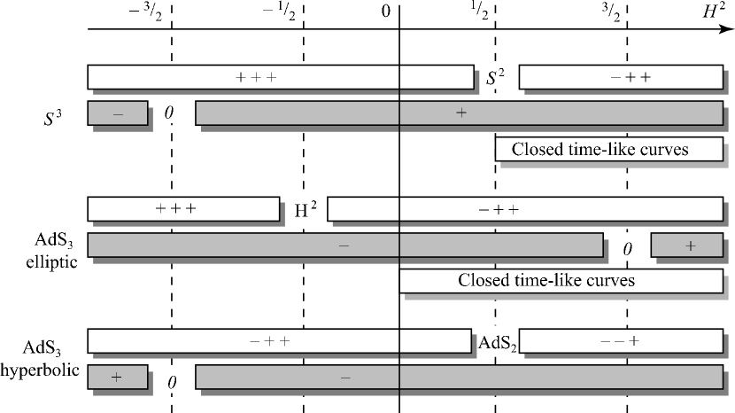
Figure 1: We have summarized the various regimes appearing in magnetic/electric deformations of the $SU\left(2\right)_{k}$ and $SL\left(2,{\mathord{\mathbb{R}}}\right)_{k}$ wzw models. Lighter bars indicate the signature, darker ones the sign of the curvature. Regions with $H^{2}<0$ have well-defined geometries with imaginary gauge field. Their string interpretation is therefore questionable.

We have presented the spectrum and the partition function of the $SU(2)_{k}$ magnetic deformation with $S^{2}\times\mathbb{R}$ as extreme target space reached at $H^{2}_{\rm max}=1/2$. At this value the fiber $S^{1}$ decompactifies, as we have seen in Sec. 2.2. We can go across and explore the deformation for $H^{2}>1/2$. The geometry (metric given in Eq. (10)) is now Lorentzian and all other fields are real. This exact solution is still a marginal deformation of $S^{3}$, of a peculiar type though: it appears after a signature flip, has positive constant curvature (see Fig. 1) and $U(1)\times SU(2)$ isometry, where some of the $SU(2)$ Killing vectors are time-like. In order to avoid trivial closed time-like curves, we must promote the angle $\gamma$ to $\gamma\in\mathbb{R}$. Unfortunately this is not enough to ensure consistency, and closed time-like curves à la Gödel appear whenever $\cos^{2}\beta>1/2H^{2}$, as one can check by using standard arguments (Sec. 3).

The space–time under consideration is a compact Gödel universe (“compact” refers to the angle $\beta$), already discussed in the context of general relativity [49]. Our approach promotes it to the level of exact string background, and we have in principle the tools to investigate its spectrum. The latter may be obtained from the partition function (27) with the replacement:

$$\cosh x=\frac{\imath}{2H^{2}-1}\ , \sinh x=\imath\sqrt{\frac{2H^{2}}{2H^{2}-1}}.$$ (84)

Such a straightforward approach is however questionable since it involves a sort of analytic continuation. We will not expand further on this issue.

The hyperbolic deformation of $SL(2,\mathbb{R})_{k}$, leading precisely to $\mathrm{AdS}_{2}$, is an important achievement of this work. It is however technically involved: no description is presently available for quantities like the partition function, and our handling over the spectrum remains incomplete. For the elliptic deformation, the partition function is available in the “Gödel regime” ($H^{2}>0$) where the geometry is spoiled by closed time-like curves. The continuation to the negative-$H^{2}$ region, free of closed time-like curves, is not straightforward since it requires an analytic continuation to imaginary magnetic field. The string theory is no longer unitary, but it might still be useful to investigate this regime for pure cft purposes.

Several other non-unitary regimes appear in the deformed geometries at hand, either with Euclidean or with Lorentzian signature, and positive or negative curvature (see Fig. 1). Whether these could be connected to the $H_{3}$ or $\mathrm{dS}_{3}$ spaces is an open question. Three-dimensional hyperbolic plane, $H_{3}$, and de Sitter, $\mathrm{dS}_{3}$, are respectively negative and positive constant-curvature symmetric spaces, with Euclidean and Lorentzian signatures. The differences with respect to the $S^{3}$ or $\mathrm{AdS}_{3}$ are that they have the opposite signature/curvature combination, and are not group manifolds: $H_{3}$ and $\mathrm{dS}_{3}$ are $SL(2,\mathbb{C})$ cosets. A non-unitary conformal sigma model can be defined on $H_{3}$, and considerable progress has been made to understand its structure. In the case of $\mathrm{dS}_{3}$, nothing similar is available, despite the growing interest for cosmological applications. Any hint in that direction could be important.

New backgrounds arise by introducing extra deformations. Since the residual affine symmetry of the asymmetric marginal deformations is $U(1)_{\rm L}\times SL(2,\mathbb{R})_{\rm R}$, there is room, at any point, for a extra modulus generated by a $U(1)_{\rm L}\times U(1)_{\rm R}\subset U(1)_{\rm L}\times SL(2,\mathbb{R})_{\rm R}$ bilinear. This freedom has been used e.g in [10] in order to cure the causal problem of the magnetic deformation (i.e. the Gödel universe), by slightly deviating from the pure magnetic line. One can readily repeat this analysis in the new regimes we have presented here, as already sketched for the parabolic deformation – end of Sec. 3.3 – and further investigate the $\mathrm{AdS}_{3}$ landscape and its connections to other three-dimensional constant-curvature spaces of physical interest.

Our analysis deserves some extra comments. We are in position now to describe $\mathrm{AdS}_{2}\times S^{2}$ as the target space of a two-dimensional conformal model. This supersymmetric setting is the near-horizon geometry of the extremal Reissner–Nordström four-dimensional black hole. In our approach, this geometry arises as a marginal deformation of the near-horizon geometry of the ns5/F1 set up ($\mathrm{AdS}_{3}\times S^{3}$). The crucial question that remains to be answered is how to deviate from this supersymmetric geometry towards a non-extremal configuration of the charged four-dimensional black hole.

We should also stress that the new string backgrounds we have constructed may have interesting applications for holography. For example, the AdS/plane-wave background (58) is a superposition of two solutions with known holographic interpretation. The line of geometries relating $\mathrm{AdS}_{3}$ and $\mathrm{AdS}_{2}$ (hyperbolic deformation), which are both candidates for AdS/cft, can possibly have some holographic dual for all values of the modulus $H^{2}$. It is important to remark that all the families of conformal field theories considered in this paper preserve one chiral $SL(2,\mathbb{R})$ affine algebra, hence allow to contruct one space–time Virasoro algebra by using the method given in [50].

Finally, concerning the general technique that we have used, it clearly opens up new possibilities for compactifications. Asymmetric deformations can be performed on any group-$G$ manifold. The high residual symmetry $G\times U(1)^{{\rm rank}\ G}$ forces the geometry along the line as well as at the boundary of the modulus. There, we are naturally led to the geometric coset $G/U(1)^{{\rm rank}\ G}$ times ${\rm rank}\ G$ decoupled, non compact, free bosons. A magnetic field drives this asymmetric deformation in the case of compact groups, whereas in non-compact cases a variety of situations can arise as we showed for the $SL(2,\mathbb{R})$ wzw model.

Appendix A Geometric deformations

In this appendix, we would like to present some selected results about geometric deformations. Since most of the material discussed in this paper deals with deformations of backgrounds that preserve part of the original isometries, it is interesting to understand how such deformations can be implemented in a controllable way. Whether these are the most general, or can be promoted to exact marginal lines in the underlying two-dimensional sigma model, are more subtle issues that we analyze in the main part of the paper for $S^{3}$ and $\mathrm{AdS}_{3}$.

Consider a manifold with metric ${\,\mathrm{d}}s^{2}=g_{\alpha\beta}{\,\mathrm{d}}x^{\alpha}{\,\mathrm{d}}x^{\beta}$. We assume the existence of an isometry generated by a Killing vector $\xi$. The components of its dual form are $\varpi_{\alpha}=g_{\alpha\beta}\xi^{\beta}$. We will consider the following family of geometries:

$$g_{\alpha\beta}^{\rm def}=g_{\alpha\beta}^{\vphantom{f}}+f\left({\|\xi\|^{2}}\right)\varpi_{\alpha}^{\vphantom{f}}\varpi_{\beta}^{\vphantom{f}}$$ (85)

with $f$ an arbitrary function of the norm of the Killing vector. Each member of the family corresponds to a specific choice of $f$.

Deformation (85) provides a simple and straightforward recipe for perturbing a background in a way that keeps under control its isometries. Indeed, the vector $\xi$ is still an isometry generator (${\mathcal{L}}_{\xi}\|\xi\|^{2}=0;\;{\mathcal{L}}_{\xi}\varpi=0$). So are all Killing vectors which commute with $\xi$, whereas for a generic $f\left(\mathinner{\left\|{\xi}\right\|}^{2}\right)$ those of the original isometry group which do not commute with $\xi$ are no longer Killing vectors. Therefore, the “deformed” isometry group contains only a subgroup of the simple component to which $\xi$ belongs, times the other simple components, if any. These symmetry properties hold for generic functions $f\left({\|\xi\|^{2}}\right)$. Accidental enhancements can occur though, where a larger subgroup of the original group is restored (at least locally).

The deformed dual form of $\xi$ is computed by using (85):

$$\varpi_{\alpha}^{\rm def}=\varpi_{\alpha}^{\vphantom{f}}\left\{1+\|\xi\|^{2}f\left({\|\xi\|^{2}}\right)\right\}.$$ (86)

Clearly, the symmetry requirement is not strong enough to reduce substantially the freedom of the deformation. We would like to focus on a specific subset of deformations for which

$$h=-\|\xi\|^{2}f\left({\|\xi\|^{2}}\right)$$ (87)

is a real constant. This family is interesting for several reasons. It is stable under repetition of the deformation: by repeating this deformation we stay in the same class, but reach a different point of it. This is a sort of integrability property that leads to a one-parameter family of continuous deformations. The value $h=1$ is a critical value of the deformation parameter. At this value the metric degenerates. This is a sign for the decoupling of one dimension. For $h>1$, the signature flips and the decoupled dimension reenters the geometry, with reversed signature though.

In the presence of Lorentzian geometries, light-like Killing vectors can also be used. For those, Eq. (85) is necessarily of the form

$$g_{\alpha\beta}^{\rm def}=g_{\alpha\beta}^{\vphantom{f}}-h\varpi_{\alpha}^{\vphantom{f}}\varpi_{\beta}^{\vphantom{f}}\ {\rm if}\ \ \|\xi\|^{2}=0.$$ (88)

The symmetry constraint is here very powerful. Furthermore, since now $\varpi_{\alpha}^{\rm def}=\varpi_{\alpha}^{\vphantom{f}}$, no critical phenomenon occurs in this case, at least for finite values of $h$.

Deformations of the kind (85) with (87) arise naturally as background geometries of integrable marginal deformations of wzw models. The integrability requirement for the cft deformation selects the above one-parameter family of geometries. In turn, these families exhibit limiting spaces.

It is useful to notice that deformations (85) with (87) become trivial if $\xi$ is of the form $\xi=\,\partial_{1}$ with $g_{\alpha\beta}$ block diagonal: $g_{\alpha 1}=g_{11}\,\delta_{\alpha 1}$. In this case, $\varpi=g_{11}{\,\mathrm{d}}x^{1}$, and $g_{\alpha\beta}$ is unaffected for $(\alpha,\beta)\neq(1,1)$, whereas $g_{11}^{\rm def}=g_{11}^{\vphantom{f}}\left(1-h\right)$. The net effect of the deformation is a rescaling of the coordinate $x^{1}$. The isometry group remains unaltered, at least locally. In fact, if $x^{1}$ is an angle ($\xi$ is a compact generator), the deformation amounts to introducing an angle deficit, which brakes globally the original isometry group to the subgroup described previously and introduces a conical singularity.

We can illustrate the latter “degenerate” situation with a simple example: the case of the two-dimensional Euclidean plane. The isometry group has three generators: one rotation and two translations. Consider the rotation and perform the deformation as in (85), (87). The resulting manifold is a cone. Although translation generators do not commute with the rotation generator, translation invariance is still a symmetry, locally – since the only effect of the rotation is to rescale the polar angle. Translation is however broken globally. The critical value of the deformation ($h=1$) corresponds to the maximal angle deficit, where the cone degenerates into a half-line.

Many deformations driven by $\xi_{(1)},\xi_{(2)},\ldots$ can be performed simultaneously along the previous lines of thought. In order to keep $\xi_{(1)},\xi_{(2)},\ldots$ in the isometry group of the deformed metric, these must commute, hence must belong to the Cartan subgroup of the original isometry group. The full deformed group also contains those among the original Killing vectors, which commute with the set $\{\xi_{(1)},\xi_{(2)},\ldots\}$.

Curvature tensors (Riemann, Ricci, Gauss) can be computed for the deformed geometries under consideration (Eq. (85)), in terms of the original ones. How much they are altered depends on the left-over symmetry and on the function $f$. We will not expand further in this direction.

Appendix B The three-sphere

The commutation relations for the generators of $SU(2)$ are

$$\mathinner{\left[{J^{1},J^{2}}\right]}=\imath J^{3} \mathinner{\left[{J^{2},J^{3}}\right]}=\imath J^{1} \mathinner{\left[{J^{3},J^{1}}\right]}=\imath J^{2}.$$ (89)

A two-dimensional realization is obtained by using the standard Pauli matrices$\sigma^{a}$: $J^{a}=\sigma^{a}/2$.

The Euler-angle parameterization for $SU(2)$ is defined as:

$$g={\rm e}^{\imath{\gamma\over 2}\sigma^{3}}{\rm e}^{\imath{\beta\over 2}\sigma^{1}}{\rm e}^{\imath{\alpha\over 2}\sigma^{3}}.$$ (90)

The $SU(2)$ group manifold is a unit-radius three-sphere. A three-sphere can be embedded in flat Euclidean four-dimensional space with coordinates $(x^{1},x^{2},x^{3},x^{4})$, as $(x^{1})^{2}+(x^{2})^{2}+(x^{3})^{2}+(x^{4})^{2}=L^{2}$. The corresponding $SU(2)$ element $g$ is the following:

$$g=L^{-1}\ \begin{pmatrix}x^{4}+\imath x^{2}&x^{3}+\imath x^{1}\\ -x^{3}+\imath x^{1}&x^{4}-\imath x^{2}\end{pmatrix}.$$ (91)

In general, the invariant metric of a group manifold can be expressed in terms of the left-invariant Cartan–Maurer one-forms. In the $SU(2)$ case under consideration (unit-radius $S^{3}$),

$$\mathcal{J}^{1}=\frac{1}{2}\,{\rm tr}\,\left(\sigma^{1}g^{-1}{\,\mathrm{d}}g\right), \mathcal{J}^{2}=\frac{1}{2}\,{\rm tr}\,\left(\sigma^{2}g^{-1}{\,\mathrm{d}}g\right), \mathcal{J}^{3}=\frac{1}{2}\,{\rm tr}\,\left(\sigma^{3}g^{-1}{\,\mathrm{d}}g\right)$$ (92)

and

$${\,\mathrm{d}}s^{2}=\sum_{i=1}^{3}\mathcal{J}^{i}\otimes\mathcal{J}^{i}$$ (93)

The volume form reads:

$$\omega_{[3]}=\mathcal{J}^{1}\land\mathcal{J}^{2}\land\mathcal{J}^{3}.$$ (94)

In the Euler-angle parameterization, Eq. (93) reads (for a radius-L three-sphere):

$${\,\mathrm{d}}s^{2}=\frac{L^{2}}{4}\left({\,\mathrm{d}}\alpha^{2}+{\,\mathrm{d}}\gamma^{2}+2\cos\beta{\,\mathrm{d}}\alpha{\,\mathrm{d}}\gamma+{\,\mathrm{d}}\beta^{2}\right),$$ (95)

whereas (94) leads to

$$\omega_{[3]}=\frac{L^{3}}{8}\sin\beta{\,\mathrm{d}}\alpha\land{\,\mathrm{d}}\beta\land{\,\mathrm{d}}\gamma.$$ (96)

The Levi–Civita connection has scalar curvature $R=6/L^{2}$.

The isometry group of the $SU(2)$ group manifold is generated by left or right actions on $g$: $g\to hg$ or $g\to gh$ $\forall h\in SU(2)$. From the four-dimensional point of view, it is generated by the rotations $\zeta_{ab}=i\left(x_{a}\partial_{b}-x_{b}\partial_{a}\right)$ with $x_{a}=\delta_{ab}x^{b}$. We list here explicitly the six generators, as well as the group action they correspond to:

$$L_{1} =\frac{1}{2}\left(-\zeta_{32}+\zeta_{41}\right), g \to\mathrm{e}^{-\imath\frac{\lambda}{2}\sigma^{1}}g,$$ (97a)

$$L_{2} =\frac{1}{2}\left(-\zeta_{43}-\zeta_{12}\right), g \to\mathrm{e}^{\imath\frac{\lambda}{2}\sigma^{2}}g,$$ (97b)

$$L_{3} =\frac{1}{2}\left(-\zeta_{31}-\zeta_{42}\right), g \to\mathrm{e}^{\imath\frac{\lambda}{2}\sigma^{3}}g,$$ (97c)

$$R_{1} =\frac{1}{2}\left(\zeta_{41}+\zeta_{32}\right), g \to g\mathrm{e}^{\imath\frac{\lambda}{2}\sigma^{1}},$$ (97d)

$$R_{2} =\frac{1}{2}\left(-\zeta_{43}+\zeta_{12}\right), g \to g\mathrm{e}^{\imath\frac{\lambda}{2}\sigma^{2}},$$ (97e)

$$R_{3} =\frac{1}{2}\left(\zeta_{31}-\zeta_{42}\right), g \to g\mathrm{e}^{\imath\frac{\lambda}{2}\sigma^{3}}.$$ (97f)

Both sets satisfy the algebra (89). The norms squared of the Killing vectors are all equal to $L^{2}/4$.

The currents of the $SU\left(2\right)_{k}$ wzw model are easily obtained as:

$$J^{i}=-k\,{\rm tr}\,\left(\imath\sigma^{i}\,\partial gg^{-1}\right) \bar{J}^{i}=-k\,{\rm tr}\,\left(\imath\sigma^{i}g^{-1}\,\bar{\partial}g\right),$$ (98)

where $L=\sqrt{k}$, at the classical level. Explicit expressions are given in Tab. 1.

sector	Killing vector	Current
left moving	$$\displaystyle\frac{\sin\gamma}{\sin\beta}\,\partial_{\alpha}+\cos\gamma\,\partial_{\beta}-\frac{\sin\gamma}{\tan\beta}\,\partial_{\gamma}$$ $$\displaystyle\frac{\cos\gamma}{\sin\beta}\,\partial_{\alpha}-\sin\gamma\,\partial_{\beta}-\frac{\cos\gamma}{\tan\beta}\,\partial_{\gamma}$$ $$\displaystyle\,\partial_{\gamma}$$	$$\displaystyle k\left(\sin\beta\sin\gamma\,\partial\alpha+\cos\gamma\,\partial b\right)$$ $$\displaystyle k\left(\cos\gamma\sin\beta\,\partial\alpha-\sin\gamma\,\partial\beta\right)$$ $$\displaystyle k\left(\,\partial\gamma+\cos\beta\,\partial\alpha\right)$$
right moving	$$\displaystyle-\frac{\sin\alpha}{\tan\beta}\,\partial_{\alpha}+\cos\alpha\,\partial_{\beta}+\frac{\sin\alpha}{\sin\beta}\,\partial_{\gamma}$$ $$\displaystyle\frac{\cos\alpha}{\tan\beta}\,\partial_{\alpha}+\sin\alpha\,\partial_{\beta}-\frac{\cos\alpha}{\sin\beta}\,\partial_{\gamma}$$ $$\displaystyle\,\partial_{\alpha}$$	$$\displaystyle k\left(\cos\alpha\,\bar{\partial}\beta+\sin\alpha\sin\beta\,\bar{\partial}\gamma\right)$$ $$\displaystyle k\left(\sin\alpha\,\bar{\partial}\beta-\cos\alpha\sin\beta\,\bar{\partial}\gamma\right)$$ $$\displaystyle k\left(\,\bar{\partial}\alpha+\cos\beta\,\bar{\partial}\gamma\right)$$

Table 1: Killing vectors $\mathinner{\{{\imath L_{1},\imath L_{2},\imath L_{3}}\}}$ and $\mathinner{\{{\imath R_{1},\imath R_{2},\imath R_{3}}\}}$, and holomorphic and anti-holomorphic currents (as defined in Eqs. (97) and (98)) in Euler angles.

Appendix C $\mathrm{AdS}_{3}$

The commutation relations for the generators of the $SL(2,\mathbb{R})$ algebra are

$$\mathinner{\left[{J^{1},J^{2}}\right]}=-\imath J^{3} \mathinner{\left[{J^{2},J^{3}}\right]}=\imath J^{1} \mathinner{\left[{J^{3},J^{1}}\right]}=\imath J^{2}.$$ (99)

The sign in the first relation is the only difference with respect to the $SU(2)$ in Eq. (89).

The three-dimensional anti-de-Sitter space is the universal covering of the $SL(2,\mathbb{R})$ group manifold. The latter can be embedded in a Lorentzian flat space with signature $(-,+,+,-)$ and coordinates $(x^{0},x^{1},x^{2},x^{3})$:

$$g=L^{-1}\ \begin{pmatrix}x^{0}+x^{2}&x^{1}+x^{3}\\ x^{1}-x^{3}&x^{0}-x^{2}\end{pmatrix},$$ (100)

where $L$ is the radius of $\mathrm{AdS}_{3}$. On can again introduce Euler-like angles

$$g=\mathrm{e}^{\imath(\tau+\varphi)\sigma_{2}/2}\mathrm{e}^{\rho\sigma_{1}}\mathrm{e}^{\imath(\tau-\varphi)\sigma_{2}/2},$$ (101)

which provide good global coordinates for $\mathrm{AdS}_{3}$ when $\tau\in]-\infty,+\infty[$, $\rho\in[0,\infty[$, and $\varphi\in[0,2\pi]$.

An invariant metric (see Eq. (93)) can be introduced on $\mathrm{AdS}_{3}$. In Euler angles, the latter reads:

$${\,\mathrm{d}}s^{2}=L^{2}\left[-\cosh^{2}\rho\,{\,\mathrm{d}}\tau^{2}+{\,\mathrm{d}}\rho^{2}+\sinh^{2}\rho\,{\,\mathrm{d}}\varphi^{2}\right].$$ (102)

The Ricci scalar of the corresponding Levi–Civita connection is $R=-6/L^{2}$.

The isometry group of the $SL(2,\mathbb{R})$ group manifold is generated by left or right actions on $g$: $g\to hg$ or $g\to gh$ $\forall h\in SL(2,\mathbb{R})$. From the four-dimensional point of view, it is generated by the Lorentz boosts or rotations $\zeta_{ab}=i\left(x_{a}\partial_{b}-x_{b}\partial_{a}\right)$ with $x_{a}=\eta_{ab}x^{b}$. We list here explicitly the six generators, as well as the group action they correspond to:

$$L_{1} =\frac{1}{2}\left(\zeta_{32}-\zeta_{01}\right), g \to\mathrm{e}^{-\frac{\lambda}{2}\sigma^{1}}g,$$ (103a)

$$L_{2} =\frac{1}{2}\left(-\zeta_{31}-\zeta_{02}\right), g \to\mathrm{e}^{-\frac{\lambda}{2}\sigma^{3}}g,$$ (103b)

$$L_{3} =\frac{1}{2}\left(\zeta_{03}-\zeta_{12}\right), g \to\mathrm{e}^{\imath\frac{\lambda}{2}\sigma^{2}}g,$$ (103c)

$$R_{1} =\frac{1}{2}\left(\zeta_{01}+\zeta_{32}\right), g \to g\mathrm{e}^{\frac{\lambda}{2}\sigma^{1}},$$ (103d)

$$R_{2} =\frac{1}{2}\left(\zeta_{31}-\zeta_{02}\right), g \to g\mathrm{e}^{-\frac{\lambda}{2}\sigma^{3}},$$ (103e)

$$R_{3} =\frac{1}{2}\left(\zeta_{03}+\zeta_{12}\right), g \to g\mathrm{e}^{\imath\frac{\lambda}{2}\sigma^{2}}.$$ (103f)

Both sets satisfy the algebra (99). The norms of the Killing vectors are the following:

$$\mathinner{\left\|{\imath L_{1}}\right\|}^{2}=\mathinner{\left\|{\imath R_{1}}\right\|}^{2}=\mathinner{\left\|{\imath L_{2}}\right\|}^{2}=\mathinner{\left\|{\imath R_{2}}\right\|}^{2}=-\mathinner{\left\|{\imath L_{3}}\right\|}^{2}=-\mathinner{\left\|{\imath R_{3}}\right\|}^{2}=\frac{L^{2}}{4}.$$ (104)

Moreover $L_{i}\cdot L_{j}=0$ for $i\neq j$ and similarly for the right set. Left vectors are not orthogonal to right ones.

The isometries of the $SL(2,\mathbb{R})$ group manifold turn into symmetries of the $SL(2,\mathbb{R})_{k}$ wzw model, where they are realized in terms of conserved currents:

$$J^{1}\left(z\right)\pm J^{3}\left(z\right) =-k\,{\rm tr}\,\left(\left(\sigma^{1}\mp\imath\sigma^{2}\right)\,\partial gg^{-1}\right), J^{2}\left(z\right) =-k\,{\rm tr}\,\left(\sigma^{3}\,\partial gg^{-1}\right),$$ (105a)

$$\bar{J}^{1}\left(\bar{z}\right)\pm\bar{J}^{3}\left(\bar{z}\right) =k\,{\rm tr}\,\left(\left(\sigma^{1}\pm\imath\sigma^{2}\right)g^{-1}\,\bar{\partial}g\right), \bar{J}^{2}\left(\bar{z}\right) =-k\,{\rm tr}\,\left(\sigma^{3}g^{-1}\,\bar{\partial}g\right).$$ (105b)

At the quantum level, these currents, when properly normalized, satisfy the following affine $SL(2,\mathbb{R})_{k}$ opa:

$$J^{3}(z)J^{3}(0) \sim-\frac{k}{2z^{2}},$$ (106a)

$$J^{3}(z)J^{\pm}(0) \sim\pm\frac{J^{\pm}}{z},$$ (106b)

$$J^{+}(z)J^{-}(0) \sim\frac{2J^{3}}{z}-\frac{k}{z^{2}},$$ (106c)

and similarly for the right movers. The central charge of the enveloping Virasoro algebra is $c=3+6/(k-2)$.

We will introduce three different coordinate systems where the structure of $\mathrm{AdS}_{3}$ as a Hopf fibration is more transparent. They are explicitly described in the following.

• The $\left(\rho,t,\phi\right)$ coordinate system used to describe the magnetic deformation in Sec. 3.1 is defined as follows:

  $$\begin{cases}\frac{x_{0}}{L}&=\cosh\frac{\rho}{2}\cosh\frac{\phi}{2}\cos\frac{t}{2}-\sinh\frac{\rho}{2}\sinh\frac{\phi}{2}\sin\frac{t}{2}\\ \frac{x_{1}}{L}&=-\sinh\frac{\rho}{2}\sinh\frac{\phi}{2}\cos\frac{t}{2}-\cosh\frac{\rho}{2}\sinh\frac{\phi}{2}\sin\frac{t}{2}\\ \frac{x_{2}}{L}&=-\cosh\frac{\rho}{2}\sinh\frac{\phi}{2}\cos\frac{t}{2}+\sinh\frac{\rho}{2}\cosh\frac{\phi}{2}\sin\frac{t}{2}\\ \frac{x_{3}}{L}&=-\sinh\frac{\rho}{2}\sinh\frac{\phi}{2}\cos\frac{t}{2}-\cosh\frac{\rho}{2}\cosh\frac{\phi}{2}\sin\frac{t}{2}.\end{cases}$$ (107)

  The metric (93) reads:

  $${\,\mathrm{d}}s^{2}=\frac{L^{2}}{4}\left({\,\mathrm{d}}\rho^{2}+{\,\mathrm{d}}\phi^{2}-{\,\mathrm{d}}t^{2}-2\sinh\rho{\,\mathrm{d}}t{\,\mathrm{d}}\phi\right)$$ (108)

  and the corresponding volume form is:

  $$\omega_{[3]}=\frac{L^{3}}{8}\cosh\rho.{\,\mathrm{d}}\rho\land{\,\mathrm{d}}\phi\land{\,\mathrm{d}}t$$ (109)

  Killing vectors and currents are given in Tab. 2. It is worth to remark that this coordinate system is such that the $t$-coordinate lines coincide with the integral curves of the Killing vector $\imath L_{3}$, whereas the $\phi$-lines are the curves of $\imath R_{2}$.

• The $\left(r,x,\tau\right)$ coordinate system used to describe the electric deformation in Sec. 3.2 is defined as follows:

  $$\begin{cases}\frac{x_{0}}{L}&=\cosh\frac{r}{2}\cosh\frac{x}{2}\cos\frac{\tau}{2}+\sinh\frac{r}{2}\sinh\frac{x}{2}\sin\frac{\tau}{2}\\ \frac{x_{1}}{L}&=-\sinh\frac{r}{2}\cosh\frac{x}{2}\cos\frac{\tau}{2}+\cosh\frac{r}{2}\sinh\frac{x}{2}\sin\frac{\tau}{2}\\ \frac{x_{2}}{L}&=-\cosh\frac{r}{2}\sinh\frac{x}{2}\cos\frac{\tau}{2}-\sinh\frac{r}{2}\cosh\frac{x}{2}\sin\frac{\tau}{2}\\ \frac{x_{3}}{L}&=\sinh\frac{r}{2}\sinh\frac{x}{2}\cos\frac{\tau}{2}-\cosh\frac{r}{2}\cosh\frac{x}{2}\sin\frac{\tau}{2}.\end{cases}$$ (110)

  For $\mathinner{\{{r,x,\tau}\}}\in\mathbb{R}^{3}$, this patch covers exactly once the whole $\mathrm{AdS}_{3}$, and is regular everywhere [36]. The metric is then given by

  $${\,\mathrm{d}}s^{2}=\frac{L^{2}}{4}\left({\,\mathrm{d}}r^{2}+{\,\mathrm{d}}x^{2}-{\,\mathrm{d}}\tau^{2}+2\sinh r{\,\mathrm{d}}x{\,\mathrm{d}}\tau\right)$$ (111)

  and correspondingly the volume form is

  $$\omega_{[3]}=\frac{L^{3}}{8}\cosh r{\,\mathrm{d}}r\land{\,\mathrm{d}}x\land{\,\mathrm{d}}\tau.$$ (112)

  Killing vectors and currents are given in Tab. 3. In this case the $x$-coordinate lines coincide with the integral curves of the Killing vector $\imath R_{2}$, whereas the $\tau$-lines are the curves of $\imath R_{3}$.

• The Poincaré coordinate system used in Sec. 3.3 to obtain the electromagnetic-wave background is defined by

  $$\begin{cases}x^{0}+x^{2}&=\frac{L}{u}\\ x^{0}-x^{2}&=Lu+\frac{Lx^{+}x^{-}}{u}\\ x^{1}\pm x^{3}&=\frac{Lx^{\pm}}{u}.\end{cases}$$ (113)

  For $\mathinner{\{{u,x^{+},x^{-}}\}}\in\mathbb{R}^{3}$, the Poincaré coordinates cover once the $SL(2\mathbb{R})$ group manifold. Its universal covering, $\mathrm{AdS}_{3}$, requires an infinite number of such patches. Moreover, these coordinates exhibit a Rindler horizon at $|u|\to\infty$; the conformal boundary is at $|u|\to 0$. Now the metric reads:

  $${\,\mathrm{d}}s^{2}=\frac{L^{2}}{u^{2}}\left({\,\mathrm{d}}u^{2}+{\,\mathrm{d}}x^{+}{\,\mathrm{d}}x^{-}\right)$$ (114)

  and the volume form:

  $$\omega_{[3]}=\frac{L^{3}}{2u^{3}}{\,\mathrm{d}}u\land{\,\mathrm{d}}x^{-}\land{\,\mathrm{d}}x^{+}.$$ (115)

  In these coordinates it is simple to write certain a linear combination of the Killing vector so to obtain explicitly a light-like isometry generator. For this reason in Tab. 4 we report the $\mathinner{\{{L_{1}+L_{3},L_{1}-L_{3},L_{2},R_{1}+R_{3},R_{1}-R_{3},R_{2}}\}}$ isometry generators and the corresponding $\mathinner{\{{J_{1}+J_{3},J_{1}-J_{3},J_{2},\bar{J}_{1}+\bar{J}_{3},\bar{J}_{1}-\bar{J}_{3},\bar{J}_{2}}\}}$ currents.

sector	Killing vector	Current
left moving	$$\displaystyle\cos t\,\partial_{\rho}+\frac{\sin t}{\cosh\rho}\,\partial_{\phi}-\sin t\tanh\rho\,\partial_{t}$$ $$\displaystyle-\sin t\,\partial_{\rho}+\frac{\cos t}{\cosh\rho}\,\partial_{\phi}-\cos t\tanh\rho\,\partial_{t}$$ $$\displaystyle-\,\partial_{t}$$	$$\displaystyle k\left(\cos t\,\partial\rho+\cosh\rho\sin t\,\partial\phi\right)$$ $$\displaystyle k\left(\cos t\cosh\rho\,\partial\phi-\sin t\,\partial\rho\right)$$ $$\displaystyle k\left(\,\partial t+\sinh\rho\,\partial\phi\right)$$
right moving	$$\displaystyle\cosh\phi\,\partial_{\rho}-\sinh\phi\tanh\rho\,\partial_{\phi}-\frac{\sinh\phi}{\cosh\rho}\,\partial_{t}$$ $$\displaystyle\,\partial_{\phi}$$ $$\displaystyle\sinh\phi\,\partial_{\rho}-\cosh\phi\tanh\rho\,\partial_{\phi}-\frac{\cosh\phi}{\cosh\rho}\,\partial_{t}$$	$$\displaystyle-k\left(\cosh\phi\,\bar{\partial}\rho+\cosh\rho\sinh\phi\,\bar{\partial}t\right)$$ $$\displaystyle k\left(\,\bar{\partial}\phi-\sinh\rho\,\bar{\partial}t\right)$$ $$\displaystyle k\left(\cosh\rho\cosh\phi\,\bar{\partial}t+\sinh\phi\,\bar{\partial}\rho\right)$$

Table 2: Killing vectors $\mathinner{\{{\imath L_{1},\imath L_{2},\imath L_{3}}\}}$ and $\mathinner{\{{\imath R_{1},\imath R_{2},\imath R_{3}}\}}$, and holomorphic and anti-holomorphic currents (as defined in Eqs. (103) and (105)) for the $\left(\rho,t,\phi\right)$ coordinate system (elliptic base).

sector	Killing vector	Current
left moving	$$\displaystyle\cosh x\,\partial_{r}-\sinh x\tanh r\,\partial_{x}+\frac{\sinh x}{\cosh r}\,\partial_{\tau}$$ $$\displaystyle\,\partial_{x}$$ $$\displaystyle-\sinh x\,\partial_{r}+\cosh x\tanh r\,\partial_{x}-\frac{\cosh x}{\cosh r}\,\partial_{\tau}$$	$$\displaystyle k\left(\cosh x\,\partial r-\cosh r\sinh x\,\partial\tau\right)$$ $$\displaystyle k\left(\,\partial x+\sinh r\,\partial\tau\right)$$ $$\displaystyle k\left(\cosh r\cosh x\,\partial\tau-\sinh x\,\partial r\right)$$
right moving	$$\displaystyle-\cos\tau\,\partial_{r}+\frac{\sin\tau}{\cosh\tau}\,\partial_{x}-\sin\tau\tanh\tau\,\partial_{\tau}$$ $$\displaystyle\frac{\left(\cos\tau+\sin\tau\tanh r\right)\,\partial_{x}+\left(\cos\tau\sinh r-\frac{\sin\tau}{\cosh r}\right)\,\partial_{\tau}}{\cosh r}$$ $$\displaystyle-\,\partial_{\tau}$$	$$\displaystyle k\left(-\cos\tau\,\bar{\partial}r+\cosh r\sin\tau\,\bar{\partial}r\right)$$ $$\displaystyle k\left(\cos\tau\cosh r\,\bar{\partial}x+\sin\tau\,\bar{\partial}r\right)$$ $$\displaystyle k\left(\,\bar{\partial}\tau-\sinh r\,\bar{\partial}x\right)$$

Table 3: Killing vectors $\mathinner{\{{\imath L_{1},\imath L_{2},\imath L_{3}}\}}$ and $\mathinner{\{{\imath R_{1},\imath R_{2},\imath R_{3}}\}}$, and holomorphic and anti-holomorphic currents (as defined in Eqs. (103) and (105)) for the $\left(r,x,\tau\right)$ coordinate system (hyperbolic base).

sector	Killing vector	Current
left moving	$$\displaystyle-\,\partial_{-}$$ $$\displaystyle ux^{-}\,\partial_{u}-u^{2}\,\partial_{+}+\left(x^{-}\right)^{2}\,\partial_{-}$$ $$\displaystyle\frac{u}{2}\,\partial_{u}+x^{-}\,\partial_{-}$$	$$\displaystyle-2k\frac{\partial x^{+}}{u^{2}}$$ $$\displaystyle 2k\left(2x^{-}\frac{\partial u}{u}-\partial x^{-}+(x^{-})^{2}\frac{\partial x^{+}}{u^{2}}\right)$$ $$\displaystyle 2k\left(\frac{\partial u}{u}+x^{-}\frac{\partial x^{+}}{u^{2}}\right)$$
right moving	$$\displaystyle\,\partial_{+}$$ $$\displaystyle-ux^{+}\,\partial_{u}-\left(x^{+}\right)^{2}\,\partial_{+}+u^{2}\,\partial_{-}$$ $$\displaystyle\frac{u}{2}\,\partial_{u}+x^{+}\,\partial_{+}$$	$$\displaystyle 2k\frac{\bar{\partial}x^{-}}{u^{2}}$$ $$\displaystyle 2k\left(-2x^{+}\frac{\bar{\partial}u}{u}+\bar{\partial}x^{+}-(x^{+})^{2}\frac{\bar{\partial}x^{-}}{u^{2}}\right)$$ $$\displaystyle 2k\left(\frac{\bar{\partial}u}{u}+x^{+}\frac{\bar{\partial}x^{-}}{u^{2}}\right)$$

Table 4: Killing vectors, and holomorphic and anti-holomorphic currents (as defined in Eqs. (103) and (105)) in Poincaré coordinates (parabolic base). The $\mathinner{\{{\imath L_{1}+\imath L_{3},\imath L_{1}-\imath L_{3},\imath L_{2},\imath R_{1}+\imath R_{3},\imath R_{1}-\imath R_{3},\imath R_{2}}\}}$ isometry generators and the corresponding $\mathinner{\{{J_{1}+J_{3},J_{1}-J_{3},J_{2},\bar{J}_{1}+\bar{J}_{3},\bar{J}_{1}-\bar{J}_{3},\bar{J}_{2}}\}}$ currents are represented so to explicitly obtain light-like isometry generators.

Appendix D Equations of motion

The general form for the marginal deformations we have studied is given by:

$$S=\frac{1}{2\pi}\int{\,\mathrm{d}}^{2}z\,\left(G^{\textsc{wzw}}_{\mu\nu}+B^{\textsc{wzw}}_{\mu\nu}\right)\partial x^{\mu}\bar{\partial}x^{\nu}+\frac{\sqrt{kk_{G}}H}{2\pi}\int{\,\mathrm{d}}^{2}z\,J\bar{J}_{G}.$$ (116)

It is not completely trivial to read off the deformed background fields that correspond to this action. In this appendix we will present a method involving a Kaluza–Klein reduction, following [51]. For simplicity we will consider the bosonic string with vanishing dilaton. The right-moving gauge current $\bar{J}_{G}$ used for the deformation has now a left-moving partner and can hence be bosonized as $\bar{J}_{G}=\imath\bar{\partial}\varphi$, $\varphi\left(z,\bar{z}\right)$ being interpreted as an internal degree of freedom. The sigma-model action is recast as

$$S=\frac{1}{2\pi}\int{\,\mathrm{d}}^{2}z\>\left(G_{\textsc{mn}}+B_{\textsc{mn}}\right)\partial x^{\textsc{m}}\bar{\partial}x^{\textsc{n}},$$ (117)

where the $x^{\textsc{m}},\textsc{m}=1,\ldots,4$ embrace the group coordinates $x^{\mu},\mu=1,2,3$ and the internal $x^{4}\equiv\varphi$:

$$x^{\textsc{m}}=\left(\begin{tabular}[]{c}$x^{\mu}$\\ \hline\cr$x^{4}$\end{tabular}\right).$$ (118)

If we split accordingly the background fields, we obtain the following decomposition:

$$G_{\textsc{mn}}=\left(\begin{tabular}[]{c|c}$G_{\mu\nu}$&$G_{\varphi\varphi}A_{\mu}$\\ \hline\cr$G_{\varphi\varphi}A_{\mu}$&$G_{\varphi\varphi}$\end{tabular}\right), B_{\textsc{m}\textsc{n}}=\left(\begin{tabular}[]{c|c}$B_{\mu\nu}$&$B_{\mu 4}$\\ \hline\cr$-B_{\mu 4}$&0\end{tabular}\right),$$ (123)

and the action becomes:

$$S=\frac{1}{2\pi}\int{\,\mathrm{d}}z^{2}\left\{\left(G_{\mu\nu}+B_{\mu\nu}\right)\,\partial x^{\mu}\,\bar{\partial}x^{\nu}+\left(G_{\varphi\varphi}A_{\mu}+B_{\mu 4}\right)\,\partial x^{\mu}\,\bar{\partial}\varphi\right.\\ \left.+\left(G_{\varphi\varphi}A_{\mu}-B_{\mu 4}\right)\,\partial\varphi\,\bar{\partial}x^{\mu}+G_{\varphi\varphi}\,\partial\varphi\,\bar{\partial}\varphi\right\}.$$ (124)

We would like to put the previous expression in such a form that space–time gauge invariance,

$$A_{\mu} \to A_{\mu}+\,\partial_{\mu}\lambda,$$ (125)

$$B_{\mu 4} \to B_{\mu 4}+\,\partial_{\mu}\eta,$$ (126)

is manifest. This is achieved as follows:

$$S=\frac{1}{2\pi}\int{\,\mathrm{d}}^{2}z\>\left\{\left(\hat{G}_{\mu\nu}+B_{\mu\nu}\right)\,\partial x^{\mu}\,\bar{\partial}x^{\nu}+B_{\mu 4}\left(\partial x^{\mu}\bar{\partial}\varphi-\partial\varphi\bar{\partial}x^{\mu}\right)\right.+\\ \left.+G_{\varphi\varphi}\left(\partial\varphi+A_{\mu}\partial x^{\mu}\right)\left(\bar{\partial}\varphi+A_{\mu}\bar{\partial}x^{\mu}\right)\right\},$$ (127)

where $\hat{G}_{\mu\nu}$ is the Kaluza–Klein metric

$$\hat{G}_{\mu\nu}=G_{\mu\nu}-G_{\varphi\varphi}A_{\mu}A_{\nu}.$$ (128)

Expression (117) coincides with (116) after the following identifications:

$$\hat{G}_{\mu\nu} =\frac{k}{2}\left(\mathcal{J}_{\mu}\mathcal{J}_{\nu}-2\textsc{h}^{2}\tilde{\mathcal{J}}_{\mu}\tilde{\mathcal{J}}_{\nu}\right)$$ (129a)

$$B_{\mu\nu} =\frac{k}{2}J_{\mu}\land J_{\nu},$$ (129b)

$$B_{\mu 4} =G_{\varphi\varphi}A_{\mu}=\textsc{h}\sqrt{\frac{kk_{g}}{2}}\tilde{\mathcal{J}}_{\mu},$$ (129c)

$$A_{\mu} =\textsc{h}\sqrt{\frac{2k}{k_{g}}}\tilde{\mathcal{J}}_{\mu},$$ (129d)

$$G_{\varphi\varphi} =\frac{k_{g}}{2}.$$ (129e)

The various backgrounds we have found throughout this paper correspond to truly marginal deformations of wzw models. Thus, they are target spaces of exact cft’s. They solve, however, the lowest-order (in $\alpha^{\prime}$) equations since all higher-order effects turn out to be captured in the shift $k\to k+2$. These $\mathcal{O}\left(\alpha^{\prime}\right)$ equations are obtained by using the bosonic action (117), or equivalently by writing the heterotic string equations of motion for the fields in (129). They read [52]:

$$\delta c =-R+\frac{k_{G}}{16}F_{\phantom{a}\mu\nu}{F}^{\mu\nu},$$ (130a)

$${\beta^{G}}_{\mu\nu} =R_{\mu\nu}^{\vphantom{n}}-\frac{1}{4}H_{\mu\rho\sigma}^{\vphantom{n}}H_{\nu}^{\phantom{\nu}\rho\sigma}-\frac{k_{G}}{4}F_{\mu\rho}^{\vphantom{n}}{F^{a}}_{\mu}^{\phantom{\mu}\rho}=0,$$ (130b)

$${\beta^{B}}_{\nu\rho} =\nabla^{\mu}_{\vphantom{n}}H_{\mu\nu\rho}^{\vphantom{n}}=0,$$ (130c)

$${\beta^{A}}_{\mu} =\nabla^{\nu}_{\vphantom{n}}F_{\mu\nu}^{\vphantom{n}}-\frac{1}{2}F^{\nu\rho}_{\vphantom{n}}H_{\mu\nu\rho}^{\vphantom{n}}=0,$$ (130d)

where

$$F_{\mu\nu} =\,\partial_{\mu}A_{\nu}-\,\partial_{\nu}A_{\mu},$$ (131)

$$H_{\mu\nu\rho} =\,\partial_{\mu}B_{\nu\rho}-\frac{k_{G}}{4}A_{\mu}F_{\nu\rho}+\text{cyclic}.$$ (132)

References

- [1] C. Kounnas, M. Porrati, and B. Rostand, On N=4 extended superLiouville theory, Phys. Lett. B258 (1991) 61–69.
- [2] J. Callan, Curtis G., J. A. Harvey, and A. Strominger, World sheet approach to heterotic instantons and solitons, Nucl. Phys. B359 (1991) 611–634.
- [3] I. Antoniadis, S. Ferrara, and C. Kounnas, Exact supersymmetric string solutions in curved gravitational backgrounds, Nucl. Phys. B421 (1994) 343–372, [hep-th/9402073].
- [4] I. Antoniadis, C. Bachas, and A. Sagnotti, Gauged supergravity vacua in string theory, Phys. Lett. B235 (1990) 255.
- [5] H. J. Boonstra, B. Peeters, and K. Skenderis, Brane intersections, anti-de Sitter spacetimes and dual superconformal theories, Nucl. Phys. B533 (1998) 127–162, [hep-th/9803231].
- [6] S. Chaudhuri and J. A. Schwartz, A criterion for integrably marginal operators, Phys. Lett. B219 (1989) 291.
- [7] S. Forste and D. Roggenkamp, Current current deformations of conformal field theories, and wzw models, JHEP 05 (2003) 071, [hep-th/0304234].
- [8] E. Kiritsis and C. Kounnas, Infrared regularization of superstring theory and the one loop calculation of coupling constants, Nucl. Phys. B442 (1995) 472–493, [hep-th/9501020].
- [9] E. Kiritsis and C. Kounnas, Infrared behavior of closed superstrings in strong magnetic and gravitational fields, Nucl. Phys. B456 (1995) 699–731, [hep-th/9508078].
- [10] D. Israël, Quantization of heterotic strings in a Gödel/anti de Sitter spacetime and chronology protection, JHEP 01 (2004) 042, [hep-th/0310158].
- [11] A. Giveon and E. Kiritsis, Axial vector duality as a gauge symmetry and topology change in string theory, Nucl. Phys. B411 (1994) 487–508, [hep-th/9303016].
- [12] C. V. Johnson, Heterotic coset models, Mod. Phys. Lett. A10 (1995) 549–560, [hep-th/9409062].
- [13] D. A. Lowe and A. Strominger, Exact four-dimensional dyonic black holes and bertotti- robinson space-times in string theory, Phys. Rev. Lett. 73 (1994) 1468–1471, [hep-th/9403186].
- [14] A. A. Tseytlin, Conformal sigma models corresponding to gauged Wess-Zumino- Witten theories, Nucl. Phys. B411 (1994) 509–558, [hep-th/9302083].
- [15] S. Ferrara, R. Kallosh, and A. Strominger, N=2 extremal black holes, Phys. Rev. D52 (1995) 5412–5416, [hep-th/9508072].
- [16] D. Kutasov, F. Larsen, and R. G. Leigh, String theory in magnetic monopole backgrounds, Nucl. Phys. B550 (1999) 183–213, [hep-th/9812027].
- [17] E. Kiritsis, Character formulae and the structure of the representations of the N=1, N=2 superconformal algebras, Int. J. Mod. Phys. A3 (1988) 1871.
- [18] V. K. Dobrev, Characters of the unitarizable highest weight modules over the N=2 superconformal algebras, Phys. Lett. B186 (1987) 43.
- [19] Y. Matsuo, Character formula of unitary representation of N=2 superconformal algebra, Prog. Theor. Phys. 77 (1987) 793.
- [20] F. Ravanini and S.-K. Yang, Modular invariance in N=2 superconformal field theories, Phys. Lett. B195 (1987) 202.
- [21] P. Berglund, C. V. Johnson, S. Kachru, and P. Zaugg, Heterotic coset models and (0,2) string vacua, Nucl. Phys. B460 (1996) 252–298, [hep-th/9509170].
- [22] S. Forste, A truly marginal deformation of SL(2, R) in a null direction, Phys. Lett. B338 (1994) 36–39, [hep-th/9407198].
- [23] D. Israël, C. Kounnas, and M. P. Petropoulos, Superstrings on NS5 backgrounds, deformed AdS(3) and holography, JHEP 10 (2003) 028, [hep-th/0306053].
- [24] R. Dijkgraaf, H. Verlinde, and E. Verlinde, String propagation in a black hole geometry, Nucl. Phys. B371 (1992) 269–314.
- [25] M. Rooman and P. Spindel, Goedel metric as a squashed anti-de sitter geometry, Class. Quant. Grav. 15 (1998) 3241–3249, [gr-qc/9804027].
- [26] M. J. Reboucas and J. Tiomno, On the homogeneity of riemannian space-times of Gödel type, Phys. Rev. D28 (1983) 1251–1264.
- [27] N. Drukker, B. Fiol, and J. Simon, Gödel’s universe in a supertube shroud, Phys. Rev. Lett. 91 (2003) 231601, [hep-th/0306057].
- [28] N. J. Vilenkin and A. Klimyk, Representation of Lie groups and special functions. Kluwer Academic Publishers, Dordrecht, 1991.
- [29] J. M. Maldacena and H. Ooguri, Strings in AdS(3) and SL(2,R) WZW model. I, J. Math. Phys. 42 (2001) 2929–2960, [hep-th/0001053].
- [30] P. M. S. Petropoulos, Comments on SU(1,1) string theory, Phys. Lett. B236 (1990) 151.
- [31] O. Aharony, M. Berkooz, D. Kutasov, and N. Seiberg, Linear dilatons, NS5-branes and holography, JHEP 10 (1998) 004, [hep-th/9808149].
- [32] M. Banados, C. Teitelboim, and J. Zanelli, The black hole in three-dimensional space-time, Phys. Rev. Lett. 69 (1992) 1849–1851, [hep-th/9204099].
- [33] M. Banados, M. Henneaux, C. Teitelboim, and J. Zanelli, Geometry of the (2+1) black hole, Phys. Rev. D48 (1993) 1506–1525, [gr-qc/9302012].
- [34] M. Natsuume and Y. Satoh, String theory on three dimensional black holes, Int. J. Mod. Phys. A13 (1998) 1229–1262, [hep-th/9611041].
- [35] S. Hemming and E. Keski-Vakkuri, The spectrum of strings on BTZ black holes and spectral flow in the SL(2,R) WZW model, Nucl. Phys. B626 (2002) 363–376, [hep-th/0110252].
- [36] O. Coussaert and M. Henneaux, Self-dual solutions of 2+1 Einstein gravity with a negative cosmological constant, hep-th/9407181.
- [37] K. Gawedzki, Noncompact WZW conformal field theories, hep-th/9110076.
- [38] J. Teschner, On structure constants and fusion rules in the SL(2,C)/SU(2) wznw model, Nucl. Phys. B546 (1999) 390–422, [hep-th/9712256].
- [39] D. Youm, Black holes and solitons in string theory, Phys. Rept. 316 (1999) 1–232, [hep-th/9710046].
- [40] N. Berkovits, M. Bershadsky, T. Hauer, S. Zhukov, and B. Zwiebach, Superstring theory on AdS(2) S(2) as a coset supermanifold, Nucl. Phys. B567 (2000) 61–86, [hep-th/9907200].
- [41] H. Verlinde, Superstrings on AdS(2) and superconformal matrix quantum mechanics, hep-th/0403024.
- [42] J. M. Maldacena, The large N limit of superconformal field theories and supergravity, Adv. Theor. Math. Phys. 2 (1998) 231–252, [hep-th/9711200].
- [43] P. Claus et. al., Black holes and superconformal mechanics, Phys. Rev. Lett. 81 (1998) 4553–4556, [hep-th/9804177].
- [44] G. W. Gibbons and P. K. Townsend, Black holes and Calogero models, Phys. Lett. B454 (1999) 187–192, [hep-th/9812034].
- [45] M. Cadoni, P. Carta, D. Klemm, and S. Mignemi, AdS(2) gravity as conformally invariant mechanical system, Phys. Rev. D63 (2001) 125021, [hep-th/0009185].
- [46] H. Ooguri, A. Strominger, and C. Vafa, Black hole attractors and the topological string, hep-th/0405146.
- [47] C. Vafa, Two dimensional yang-mills, black holes and topological strings, hep-th/0406058.
- [48] D. Gepner, Space-time supersymmetry in compactified string theory and superconformal models, Nucl. Phys. B296 (1988) 757.
- [49] N. Drukker, B. Fiol, and J. Simon, Goedel-type universes and the Landau problem, hep-th/0309199.
- [50] A. Giveon, D. Kutasov, and N. Seiberg, Comments on string theory on AdS(3), Adv. Theor. Math. Phys. 2 (1998) 733–780, [hep-th/9806194].
- [51] G. T. Horowitz and A. A. Tseytlin, A new class of exact solutions in string theory, Phys. Rev. D51 (1995) 2896–2917, [hep-th/9409021].
- [52] E. S. Fradkin and A. A. Tseytlin, Quantum string theory effective action, Nucl. Phys. B261 (1985) 1–27.