Perturbative Study of Bremsstrahlung and Pair-Production by
Spin-$\frac{1}{2}$ Particles in the Aharonov-Bohm Potential

Abstract

In the presence of an external Aharonov-Bohm potential, we investigate the two QED processes of the emission of a bremsstrahlung photon by an electron, and the production of an electron-positron pair by a single photon. Calculations are carried out using the Born approximation within the framework of covariant perturbation theory to lowest non-vanishing order in $\alpha$. The matrix element for each process is derived, and the corresponding differential cross-section is calculated. In the non-relativistic limit, the resulting angular and spectral distributions and some polarization properties are considered, and compared to results of previous works.

I Introduction

The Aharonov-Bohm (AB) effect Aharonov and Bohm (1959) is one of the remarkable predictions of quantum theory. It has shown that, contrary to classical electrodynamics, enclosed electromagnetic fields can interact with charged quantum particles via the vector potential leading to observable effects, even in the absence of Lorentz forces. Comprehensive reviews covering many aspects of the subject are Olariu and Popescu (1985); Peshkin and Tonomura (1989).

Traditionally, the AB effect has been studied in connection with elastic scattering and bound state problems. In recent years, however, a limited number of works have been devoted to processes that go beyond these problems and that open the way for a deeper, more detailed understanding of the AB effect. The two processes that have been addressed by these works were the emission of a single bremsstrahlung photon by a charged particle, and the production of particle-antiparticle pair in the AB potential. The first of these works Serebryanyi and Skarzhinskii (1988), investigated the emission of bremsstrahlung by a spinless non-relativistic particle by looking at the spectral and angular distribution of emitted photons. Then the same process was studied relativistically in Gal’tsov and Voropaev (1990) using Klein-Gordon particles, this time the polarization of the emitted photon was taken into account, and both non-relativistic and ultra-relativistic limits of the results were considered. For relativistic spin-$\frac{1}{2}$ electrons, the process was investigated in reference Audretsch et al. (1996) for Dirac particles, where the differential cross-section and its limiting cases were used to discuss spectral and angular distributions of emitted photons. That study included electron spin polarization and its effect on the polarization of the emitted photon, and angular momentum selection rules were reported.

As for the process of pair-production in the AB potential, only two studies have been conducted: the first was Skarzhinsky et al. (1996), where the differential cross-section was found and the effect of photon polarization on spin polarization of created particles was considered. Here also, angular momentum selection rules for angular momentum were reported. The case of spinless pair-production has been recently studied in Shahin , where the photon-polarized differential cross-section was calculated, and selection rules found.

In all of these works, the method of finding the scattering amplitude uses exact wavefunctions of the Klein-Gordon or Dirac particles in the AB potential, and then the scattering matrix is calculated to first order using scattering states constructed from these functions.

The aim of the present paper is to study the processes of bremsstrahlung and pair-production in an external AB potential in the Born approximation using covariant perturbation theory to the lowest non-vanishing order, which corresponds in this case to $\mathcal{O}(\alpha^{2})$. The present work was motivated by the series of works by Skarzhinsky et al. Audretsch et al. (1996); Skarzhinsky et al. (1996); Audretsch and Skarzhinsky (1998), and in that respect, the motivation was twofold: first, we think it is interesting, as such, to treat the problem using this method, as it is the one traditionally employed in this kind of calculation, where results are cast into the familiar Bethe-Heitler form, and to our knowledge, no such calculation has been reported for the AB potential. Another reason, is to test the applicability of the Born approximation to this particular problem by comparing with the results of the “exact” approach, especially since there were some speculations regarding the applicability of the small field approximation to this problem Skarzhinsky and Audretsch (1997); Audretsch and Skarzhinsky (1998).

We will use the idealization usually followed in describing the AB-potential, namely to assume it is generated by a very thin, very long flux tube putting out a potential given by:

$$A^{\mu}(x)=\frac{\Phi}{2\pi(x^{2}+y^{2})}(0,-y,x,0)$$ (1)

so that the direction of magnetic field generating the flux $\Phi$ is along the $z$-axis. In terms of the magnetic flux quantum $\Phi_{0}=2\pi/\left|e\right|$, we can write $\Phi/\Phi_{0}\equiv\delta+N$, where $N$ is the integral part and $\delta$ is the remaining fraction. To use the Born approximation, we will assume the flux to be small enough, so that $N=0$ and $\delta\ll 1$.

This paper is organized into four sections: following this introductory section, we present in section II the calculation of the matrix element and differential cross-section for the emission of a bremsstrahlung photon from a Dirac particle in the AB-potential. We also calculate the differential cross-section in the non-relativistic limit.

In section III we conduct an analogous study for the process of production of a Dirac pair in the AB-potential, where the matrix element is found and the corresponding differential cross-section is calculated. The limit of low energy photon is found as well, and the polarization effects are investigated.

Section IV summarizes our results and states the conclusions and the problems that are still open.

As regards conventions, we follow those of ref. Itzykson and Zuber (1980), specifically, we use the Pauli-Dirac representation of the $\gamma$-matrices.

II Bremsstrahlung in the AB potential

II.1 Amplitude and Cross-section

The probability amplitude for the emission of a single bremsstrahlung photon is given by the matrix element:

$$S_{fi}=\langle e^{-}\gamma|\hat{S}|e^{-}\rangle$$ (2)

The two diagrams that contribute to the process at tree-level are shown in figure (1), their sum gives us the amplitude to lowest non-vanishing order in $\alpha$ ($\mathcal{O}(\alpha^{2})$):

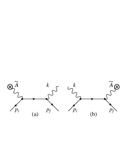
Figure 1: Tree-level diagrams for bremsstrahlung.

$$S^{(2)}_{fi}=-ie^{2}\bar{u}^{(\beta)}(p_{f})\Big{[}\not\!\epsilon^{(\lambda)*}\frac{\not\!p_{f}+\not\!k+m}{2p_{f}\cdot k}\not\!\!\tilde{A}^{\mathrm{ext}}(q)-\not\!\!\tilde{A}^{\mathrm{ext}}(q)\frac{\not\!p_{i}-\not\!k+m}{2p_{i}\cdot k}\not\!\epsilon^{(\lambda)*}\Big{]}u^{(\alpha)}(p_{i})$$ (3)

where $u^{(s)}(p)$ is a 4-component spinor satisfying the free Dirac equation for a particle with 4-momentum $p$ and in a spin state $s$. $p_{i}$, $p_{f}$, and $k$ refer to the 4-momenta of the incoming and outgoing Dirac particles, and the photon, respectively. $\epsilon_{\mu}^{(\lambda)}$ is the photon polarization vector, and $\tilde{A}_{\mu}^{\mathrm{ext}}(q)$ is the Fourier transform of the AB-potential:

$$\tilde{A}_{\mu}^{\mathrm{ext}}(q)=-\frac{(2\pi)^{2}i\Phi}{\left|\mathbf{q}\right|^{2}}\delta(q^{0})\delta(q^{3})R_{\mu}$$ (4)

Here, the momentum transfer 4-vector $q^{\mu}$ is given by:

$$q^{\mu}=p_{f}^{\mu}+k^{\mu}-p_{i}^{\mu}$$ (5)

and $R^{\mu}$ is a vector defined by:

$$R^{\mu}\equiv\big{(}0,\hat{z}\times\mathbf{q}\big{)}=(0,-q^{2},q^{1},0)$$ (6)

The nature of the problem implies that the energy is conserved ($q^{0}=0$) and that the momentum along the flux tube’s axis is also conserved ($q^{3}=0$), whereas the radial component $q^{\bot}$ is not, and momentum must be transferred to the tube. These considerations are expressed in the two $\delta$-functions appearing in (4). Now, writing (3) with the help of (4), we get:

$$\begin{aligned} S_{fi}^{(2)}&\equiv\Lambda\bar{u}^{(\beta)}(p_{f})F^{(\lambda)}u^{(\alpha)}(p_{i})\\ &=\Lambda\bar{u}^{(\beta)}(p_{f})\Big{[}\not\!\epsilon^{(\lambda)*}\frac{\not\!p_{f}+\not\!k+m}{2p_{f}\cdot k}\not\!\!R-\not\!\!R\frac{\not\!p_{i}-\not\!k+m}{2p_{i}\cdot k}\not\!\epsilon^{(\lambda)*}\Big{]}u^{(\alpha)}(p_{i})\end{aligned}$$ (7)

where $\Lambda\equiv-(2\pi e)^{2}\Phi\delta(q^{0})\delta(q^{3})/\left|{\bf{q}}\right|^{2}$, and the indices $\alpha$, $\beta$ and $\lambda$ stand for polarization states of the incoming and outgoing Dirac particles and the photon, respectively. The differential cross-section per unit length of the solenoid resulting from this amplitude, as calculated according to the conventions of Itzykson and Zuber (1980), reads:

$$d\sigma_{(\alpha\rightarrow\beta;\lambda)}=\frac{|\Lambda|^{2}}{|\mathbf{p}_{i}|/m}\Big{(}\frac{md^{3}p_{f}}{p_{f}^{0}(2\pi)^{3}}\Big{)}\Big{(}\frac{d^{3}k}{2\omega(2\pi)^{3}}\Big{)}\operatorname{tr}\left\{{\mathcal{P}_{i}^{(\alpha)}\bar{F}^{(\lambda)}\mathcal{P}_{f}^{(\beta)}F^{(\lambda)}}\right\}$$ (8)

Here $\mathcal{P}^{(s)}=u^{(s)}(p)\bar{u}^{(s)}(p)$ is an appropriate projection operator, $F^{(\lambda)}$ is as defined in (7), and $\bar{F}^{(\lambda)}=\gamma^{0}F^{(\lambda){\dagger}}\gamma^{0}$. We will be using the formula in (8) twice; once to evaluate the differential cross-section for unpolarized electrons, and once for polarized electrons. The calculations are straightforward, but quite lengthy, especially in the polarized case. The traces in either case were evaluated with the help of a computer programme called FeynPar West (1993), which runs on Mathematica. The raw output of FeynPar was then rearranged by hand to become compact and physically transparent.

In the unpolarized case $\mathcal{P}^{(s)}$ projects over positive energy states, whereas in the polarized case it further projects over states with well-defined spin polarization. For the former the effect of polarization is cancelled out by summing over states of the outgoing particle and averaging over those of the incoming particle, and the resulting projector is well-known (e.g. see Itzykson and Zuber (1980)):

$$\bar{\mathcal{P}}=\sum\limits_{s}{u^{\left(s\right)}\left(p\right)\bar{u}^{\left(s\right)}\left(p\right)}=\frac{(\not\!p+m)}{2m}$$ (9)

Plugging this projector into (8), and integrating out the $\delta$-functions, we get an unpolarized cross-section that is differential in the azimuthal angle of the outgoing electron $\varphi_{f}$, the photon momentum $\left|\mathbf{k}\right|\equiv\omega$, and the solid angle for the photon $\Omega_{\gamma}$:

$${\frac{{d\bar{\sigma}_{(\lambda)}}}{{d\varphi_{f}d\omega d\Omega_{\gamma}}}}=A+B$$ (10a)

where:

$$A =\frac{{2e^{2}(\pi\delta)^{2}\omega}}{{(2\pi)^{4}\left|{{\mathbf{p}}_{i}}\right|\left|{\mathbf{q}}\right|^{4}}}\left|{\frac{{(\epsilon^{(\lambda)}\cdot p_{f})(R\cdot p_{i})}}{{p_{f}\cdot k}}}\right.\left.{-\frac{{(\epsilon^{(\lambda)}\cdot p_{i})(R\cdot p_{f})}}{{p_{i}\cdot k}}-R\cdot\epsilon^{(\lambda)}}\right|^{2}\hfill$$ (10b)

$$B =\frac{{e^{2}(\pi\delta)^{2}\omega}}{{2(2\pi)^{4}\left|{{\mathbf{p}}_{i}}\right|}}\left[{\left|{\frac{{\epsilon^{(\lambda)}\cdot p_{f}}}{{p_{f}\cdot k}}-\frac{{\epsilon^{(\lambda)}\cdot p_{i}}}{{p_{i}\cdot k}}}\right|^{2}}\right.\left.{+\frac{{\left({k^{\bot}}\right)^{2}}}{{(p_{f}\cdot k)(p_{i}\cdot k)}}}\right]$$

$k^{\bot}$ being the radial part of $\mathbf{k}$, and the bar over $\sigma$ means that this stands for the unpolarized cross-section.

To find the polarized differential cross-section, we need to use concrete wavefunctions that describe particles in well-defined states of spin polarization. To this end, we chose wavefunctions that are eigencvectors of the 3rd component of the spin pesudotensor $\hat{S}^{\mu}$ Sokolov and Ternov (1986):

$${\hat{S}^{3}=\beta\Sigma^{3}+\frac{{p^{3}}}{m}\gamma^{5}}$$ (11)

where, $\beta$, $\Sigma^{3}$ and $\gamma^{5}$ are the usual matrices, to be used in our case in the Pauli-Dirac representation, and $p^{3}$ is the $z$-component of the momentum vector. This operator has the benefit of reducing to the usual spin projection in the non-relativistic limit. It has also been used in the works with which we shall be comparing our results Audretsch et al. (1996); Skarzhinsky et al. (1996). The free Dirac wavefunction $psi$ that can be used to construct the projector $\mathcal{P}$ will satisfy the following combined eigenvalue problem:

$$\begin{array}[]{*{20}c}{\hat{H}\psi=E\psi,}&{\hat{p}^{3}\psi=p^{3}\psi,}&{\hat{S}^{3}\psi=s\psi.}\\ \end{array}$$ (12)

where $\hat{H}$ is the free Dirac Hamiltonian, and $s$, the eigenvalue of $\hat{S}^{3}$, which takes the values $\pm\sqrt{1+\left({p^{3}/m}\right)^{2}}$. The desired functions (with normalization $\int{\bar{\psi}_{j}\psi_{j^{\prime}}}=\delta_{jj^{\prime}}$) are:

$$\psi_{j}(p)=e^{-ip\cdot x}u_{j}$$ (13a)

where the spinor part $$u_{j}$$ is given by:

$$u_{j}(p)=\frac{1}{{2\sqrt{ms}}}\left({\begin{array}[]{*{20}c}{\sqrt{E+sm}\sqrt{s+1}}\\ {\epsilon_{3}\sqrt{E-sm}\sqrt{s-1}e^{i\varphi_{p}}}\\ {\epsilon_{3}\sqrt{E+sm}\sqrt{s-1}}\\ {\sqrt{E-sm}\sqrt{s+1}e^{i\varphi_{p}}}\\ \end{array}}\right)$$ (13b)

in this equation, $\epsilon_{3}=\operatorname{sgn}(s)\operatorname{sgn}(p^{3})$, and $j$ stands for the set of quantum numbers $(E,p^{3},s)$, and the resulting projection operator then becomes:

$$u_{j}\bar{u}_{j}\equiv{\mathcal{P}}_{+}^{(s)}(p)=\frac{1}{{4sm}}\left({\not\!p+m}\right)\left({s-\gamma^{5}\gamma^{3}-\frac{{p^{3}}}{m}\gamma^{5}}\right)$$ (14)

The polarized cross-section is obtained by plugging (14) into (8). This calculation is greatly facilitated if we rewrite $F^{(\lambda)}$ appearing in (7) in terms of the following quantities (in which the index $(\lambda)$ is omitted for brevity):

$$\begin{array}[]{*{20}c}{V^{\mu}\equiv a\epsilon^{\mu*}+\left({b-c}\right)\eta^{\mu*},}&{U\equiv-\left({b+c}\right)\epsilon^{3*}},\\ \end{array}$$ (15a)

where:

$$a \equiv\frac{R\cdot p_{i}}{p_{f}\cdot k}-\frac{R\cdot p_{f}}{p_{i}\cdot k}, b \equiv-\frac{|\mathbf{q}|^{2}}{2}\frac{1}{p_{f}\cdot k},$$

$$c \equiv\frac{|\mathbf{q}|^{2}}{2}\frac{1}{p_{i}\cdot k}, {\eta}^{\mu} \equiv(0,\hat{z}\times\bm{\epsilon})=(0,-{\epsilon}^{2},{\epsilon}^{1},0).$$ (15b)

Doing this, we end up with the following:

$$\operatorname{tr}\left\{{\mathcal{P}_{i}^{(s)}\bar{F}^{(\lambda)}\mathcal{P}_{f}^{(r)}F^{(\lambda)}}\right\}=\frac{{1}}{{16rsm^{2}}}\left({J_{1}+J_{2}+J_{2}^{*}+J_{3}}\right)$$ (16a)

where

$$\begin{split}J_{1}&=4\left\{{\left[{\left({V^{*}\cdot p_{f}}\right)\left({V\cdot p_{i}}\right)+\left({V^{*}\cdot p_{i}}\right)\left({V\cdot p_{f}}\right)}\right.}\right.\\ &\quad\left.{+V^{*}\cdot V\left({m^{2}-p_{i}\cdot p_{f}}\right)}\right]\left({1+rs+\frac{{p_{f}^{3}p_{i}^{3}}}{{m^{2}}}}\right)+V^{*}\cdot V\left({k^{3}}\right)^{2}\\ &\quad+\frac{i}{m}\epsilon_{\alpha\beta\gamma\delta}p_{f}^{\alpha}p_{i}^{\beta}V^{\gamma*}V^{\delta}\left({sp_{f}^{3}+rp_{i}^{3}}\right)-im\omega\left({r+s}\right)\left({{\mathbf{V}}^{*}\times{\mathbf{V}}}\right)\\ &\quad+2\left|{V^{3}}\right|^{2}\left({m^{2}-p_{i}\cdot p_{f}}\right)\left.{-k^{3}\left[{V^{3*}V\cdot\left({p_{i}-p_{f}}\right)+V^{3}V^{*}\cdot\left({p_{i}-p_{f}}\right)}\right]}\right\}\\ \end{split}$$ (16b)

$$\begin{split}J_{2}&=4U\left\{{\frac{i}{m}\left({rp_{i}^{3}+sp_{f}^{3}}\right)\left({p_{i}^{0}V^{*}\cdot p_{f}+p_{f}^{0}V^{*}\cdot p_{i}}\right)}\right.-rs\left({{\mathbf{p}}_{i}\times{\mathbf{p}}_{f}}\right)\cdot{\mathbf{V}}^{*}\\ &\quad+p_{f}^{3}s^{2}\left({{\mathbf{V}}^{*}\times{\mathbf{p}}_{f}}\right)\cdot\hat{z}-p_{i}^{3}r^{2}\left({{\mathbf{V}}^{*}\times{\mathbf{p}}_{i}}\right)\cdot\hat{z}\\ &\quad\left.{+V^{3*}\left[{im\omega\left({r-s}\right)+\left({1-\frac{{p_{f}^{3}p_{i}^{3}}}{{m^{2}}}}\right)\left({{\mathbf{p}}_{i}\times{\mathbf{p}}_{f}}\right)\cdot\hat{z}}\right]}\right\}\hfill\\ \end{split}$$ (16c)

$$\begin{split}J_{3}&=4\left|U\right|^{2}\left\{{\left({rs-1+\frac{{p_{i}^{3}p_{f}^{3}}}{{m^{2}}}}\right)\left[{p_{i}\cdot p_{f}+2{\mathbf{p}}_{i}\cdot{\mathbf{p}}_{f}-m^{2}}\right]}\right.\left.{+\left({p_{f}^{3}+p_{i}^{3}}\right)^{2}}\right\}\end{split}$$ (16d)

In these expressions $s$ and $r$ stand for the pseudo-spin eigenvalues for the incoming and outgoing particles, respectively. We can simplify (16), without loss of generality, by assuming the electron to be incident normally on the solenoid, i.e.

$$p_{i}^{3}\equiv 0~{}\Rightarrow~{}p_{f}^{3}=-k^{3}$$ (17)

As a result of this condition, $s$ takes on the values $\pm 1$, thereby exhibiting a behaviour much like the usual spin projection. Further simplification is possible by an appropriate choice of the polarization vectors for the emitted photon. We will use the following vectors, which are constructed in a way that takes advantage of the direction of the magnetic field in the tube Sokolov and Ternov (1986):

$$\begin{split}\epsilon^{\left(\sigma\right)}&=\left({0,-\sin\varphi_{k},\cos\varphi_{k},0}\right)\\ \epsilon^{\left(\pi\right)}&=\left({0,-\cos\theta_{k}\cos\varphi_{k},-\cos\theta_{k}\sin\varphi_{k},\sin\theta_{k}}\right)\end{split}$$ (18)

where $\theta_{k}$ and $\varphi_{k}$ are the polar and azimuthal angles of the the photon’s momentum vector, respectively. From these linear polarization vectors we can construct vectors describing circular polarization: $\epsilon^{\left(\ell\right)}=\left({\epsilon^{\left(\sigma\right)}+i\ell\epsilon^{\left(\pi\right)}}\right)/\sqrt{2}$.

In terms of the unpolarized cross-section as given in (10), the polarized cross-section reads now:

$$\begin{split}\frac{{d\sigma_{\left({s\to r,\lambda}\right)}}}{{d\omega d\Omega_{\gamma}d\varphi_{f}}}&=\frac{{1+rs}}{{2rs}}\left({\frac{{d\bar{\sigma}_{\left(\lambda\right)}}}{{d\omega d\Omega_{\gamma}d\varphi_{f}}}}\right)+\frac{{e^{2}(\pi\delta)^{2}\omega}}{{(2\pi)^{4}sr\left|{{\mathbf{p}}_{i}}\right|\left|{\mathbf{q}}\right|^{4}}}\left\{{\tfrac{1}{2}\left({V\cdot V}\right)\left({k^{3}}\right)^{2}}\right.\\ &\quad+\left({V^{3}}\right)^{2}\left({m^{2}-p_{i}\cdot p_{f}}\right)-k^{3}V^{3}V\cdot\left({p_{i}-p_{f}}\right)\\ &\quad+U\left[\left({{\mathbf{p}}_{i}\times{\mathbf{p}}_{f}}\right)\cdot{\mathbf{V}}-k^{3}\left({{\mathbf{V}}\times{\mathbf{p}}_{f}}\right)\cdot\hat{z}+V^{3}\left({{\mathbf{p}}_{i}\times{\mathbf{p}}_{f}}\right)\cdot\hat{z}\right]\\ &\quad\left.{+U^{2}\left[{\tfrac{1}{2}\left({k^{3}}\right)^{2}-\left({p_{i}\cdot p_{f}+2{\mathbf{p}}_{i}\cdot{\mathbf{p}}_{f}-m^{2}}\right)}\right]}\right\}\\ \end{split}$$ (19)

II.2 Non-relativistic limit

To make the above expression more informative, we consider its behaviour in the non-relativistic limit, which gives us a clearer physical insight and an ability to compare with the results of other works.

If the incident electron is moving non-relativistically ($v\ll 1$), then the emitted photon will be soft ($\omega\rightarrow 0$). The non-relativistic limit of (19) is most easily obtained if we go back to (16), and use it to rewrite the unpolarized cross-section in terms of $V^{\mu}$ and $U$. Then, we need the following approximate forms when $v\ll 1$:

$${p\cdot k}\cong\omega m, {\mathbf{R}}\cdot{\mathbf{p}}_{f}\cong{\mathbf{R}}\cdot{\mathbf{p}}_{i}\cong p_{i}^{\bot}p_{f}^{\bot}\sin\varphi_{if}$$ (20)

$${V^{\mu}}\cong\frac{\left|\mathbf{q}\right|^{2}}{m\omega}\epsilon^{\mu*}, {U}\cong 0,$$

$$\left|s\right|\cong\left|r\right|\cong 1, \frac{1+rs}{2rs}\cong\left\{{\begin{array}[]{*{20}c}1,&\mathrm{if~{}}r=s\\ 0,&\mathrm{if~{}}r\neq s\\ \end{array}}\right\}\equiv\Theta(rs),$$

$$\frac{E_{i}E_{f}-m^{2}}{{(p_{i}^{\bot}})^{2}}\cong\frac{1}{2}\left(1+\xi^{2}\right)$$

where $\xi=\sqrt{1-\omega/(E_{i}-m)}$. Upon substituting these relations in (19), and keeping only the dominant terms, we get for the various states of polarizations:

$$\mathop{\lim}\limits_{v\to 0}\frac{{d\sigma_{\left({s\to r,\sigma}\right)}}}{{d\omega d\Omega_{\gamma}d\varphi_{f}}} =\frac{{e^{2}\left({\pi\delta}\right)^{2}v}}{{32\pi^{4}m\omega}}\Theta\left({rs}\right)\left[{\left({1+\xi^{2}}\right)+2\xi\cos\left({\varphi_{fk}+\varphi_{ik}}\right)}\right]$$ (21a)

$$\mathop{\lim}\limits_{v\to 0}\frac{{d\sigma_{\left({s\to r,\pi}\right)}}}{{d\omega d\Omega_{\gamma}d\varphi_{f}}} =\frac{{e^{2}\left({\pi\delta}\right)^{2}v}}{{32\pi^{4}m\omega}}\Theta\left({rs}\right)\cos^{2}\theta_{k}\left[{\left({1+\xi^{2}}\right)-2\xi\cos\left({\varphi_{fk}+\varphi_{ik}}\right)}\right]$$ (21b)

$$\mathop{\lim}\limits_{v\to 0}\frac{{d\sigma_{\left({s\to r,\ell}\right)}}}{{d\omega d\Omega_{\gamma}d\varphi_{f}}} =\frac{{e^{2}\left({\pi\delta}\right)^{2}v}}{{64\pi^{4}m\omega}}\Theta\left({rs}\right)\left[{\left({1+\xi^{2}}\right)\left({1+\cos^{2}\theta_{k}}\right)}\right.\hfill$$

$$\left.{+2\xi\cos\left({\varphi_{fk}+\varphi_{ik}}\right)\sin^{2}\theta_{k}-2\ell\left({\frac{{2\omega}}{{mv^{2}}}}\right)\cos\theta_{k}}\right]$$ (21c)

Some observations on these results are in order here:

1.

The factor $1/\omega$ implies the well-known infrared catastrophe in the case of a soft photon $\omega\rightarrow 0$.

2.

The appearance of the step function $\Theta(rs)$ means that the spin projection of the electron is conserved in the process of emission. But notice from (19), that at higher energies spin-flip is not prohibited.

3.

For $\pi$-polarized states, we see the factor $\cos^{2}\theta_{k}$, which is typical in this limit.

Expressions analogous to the first two equations in (21) have been arrived at by Audretsch et al. Audretsch et al. (1996), using Dirac particles, and to the third by Gal’tsov and Voropaev Gal’tsov and Voropaev (1990), using Klein-Gordon particles. Upon comparison, it is seen that Audretsch’s results readily reduce to (21a) and (21b) by setting $\delta$ to zero everywhere except in the $\sin^{2}(\pi\delta)$ factor, which appears in our case as $\left(\pi\delta\right)^{2}$. Similar steps applied to Gal’tov’s result (which is quoted as a differential cross-section integrated over azimuthal angles), reduces to our result for circular polarization when we integrate it over azimuthal angles. In comparing with Gal’tsov, however, one should note that the term $\sim\xi\cos\left(\varphi_{fk}+\varphi_{ik}\right)$ is not present their result, as this term appears as a result of the inclusion of the spin degree of freedom, a fact that was noted also in Audretsch et al. (1996). Expectedly, our approach causes some information loss in the non-relativistic limit, when compared to Audretsch’s and Gal’tsov’s results, but it does agree in the general form and characteristics. The differences lie in details of how spin, flux, and momentum enter the cross-section. For instance, Audretsch’s result predicts a certain asymmetry in the effect of the spin state due to the interaction between spin and the magnetic field. Obviously this is lacking in our cross-section at this limit. However, when the “exact” results are expanded in terms of $\delta$ with the lowest non-vanishing order kept, they coincide exactly with our expressions.

III Pair-production in the AB potential

III.1 Amplitude and Cross-section

Turning now to the process of pair-production, we start with the matrix element:

$$S_{fi}=\left\langle{e^{-}e^{+}}\right|\hat{S}\left|\gamma\right\rangle$$ (22)

The lowest non-vanishing order of this amplitude is given by the sum of the two diagrams of figure (2):

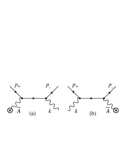
Figure 2: Tree-level diagrams for pair-production.

The processes of pair-production and bremsstrahlung are connected by a crossing symmetry, which enables us to get the expressions describing pair-production by appropriately modifying those for bremsstrahlung. The matrix element and the subsequent calculations for pair-production shall be conducted by transforming those of bremsstrahlung according to the following rules:

$$\begin{array}[]{*{20}c}{p_{i}\leftrightarrow-p_{+},}&{p_{f}\leftrightarrow p_{-},}&{k\leftrightarrow-k,}&{\epsilon^{*}\leftrightarrow\epsilon.}\\ \end{array}$$ (23)

where $p_{-}$, $p_{+}$ and $k$ are the momenta of the electron, positron, and pair-producing photon, respectively. Accordingly, we have: $q^{\mu}=p_{-}^{\mu}+p_{+}^{\mu}-k^{\mu}$ (other quantities used here without definition retain the definitions used in connection with bremsstrahlung). The sign difference between the matrix element obtained by the crossing symmetry, and that obtained using the process’s own diagrams is due to the phase convention, and can be safely dropped Peskin and Schroeder (1995). We may thus write down the matrix element for pair-production in the AB potential immediately using (7):

$$S_{fi}^{(2)}=\Lambda\bar{u}^{(\alpha)}(p_{-})\Big{[}\not\!\epsilon^{(\lambda)}\frac{\not\!p_{-}-\not\!k+m}{p_{-}\cdot k}\not\!\!R+\not\!\!R\frac{\not\!k-\not\!p_{+}+m}{p_{+}\cdot k}\not\!\epsilon^{(\lambda)}\Big{]}v^{(\beta)}(p_{+})$$ (24)

where $u^{(\alpha)}$ and $v^{(\beta)}$ are free-particle “positive-energy” and “negative-energy” solutions of Dirac’s equation, respectively, with indices $\alpha$ and $\beta$ referring to polarization states. The corresponding differential cross-section is obtained by the formula:

$$d\sigma_{(\lambda\rightarrow\alpha,\beta)}=\frac{|\Lambda|^{2}}{2\omega}\Big{(}\frac{md^{3}p_{-}}{p_{-}^{0}(2\pi)^{3}}\Big{)}\Big{(}\frac{md^{3}p_{+}}{p_{+}^{0}(2\pi)^{3}}\Big{)}\operatorname{tr}\left\{{\mathcal{P}_{+}^{(\beta)}\bar{F}^{(\lambda)}\mathcal{P}_{-}^{(\alpha)}F^{(\lambda)}}\right\}$$ (25)

As in the bremsstrahlung case, we start with evaluating this expression by neglecting the polarization of the created particles, in which case we sum over polarization states $\alpha$ and $\beta$. The projectors in this case, which project over states of positive- and negative-energy, respectively, are:

$$\bar{\mathcal{P}}_{-}=\frac{\not\!p_{-}+m}{2m},~{}~{}\bar{\mathcal{P}}_{+}=\frac{-\not\!p_{+}+m}{2m}$$ (26)

Plugging these into (25), and doing steps analogous to what was done to get (10), we end up with:

$${\frac{{d\bar{\sigma}_{(\lambda)}}}{{dp_{+}^{0}dp_{+}^{3}d\varphi_{+}d\varphi_{-}}}}=\tilde{A}+\tilde{B}$$ (27a)

where:

$$\tilde{A} =\frac{{-4e^{2}(\pi\delta)^{2}}}{{(2\pi)^{4}\left|{\mathbf{q}}\right|^{4}\omega}}\left|{\frac{{(\epsilon^{(\lambda)}\cdot p_{-})(R\cdot p_{+})}}{{p_{-}\cdot k}}}\right.\left.{+\frac{{(\epsilon^{(\lambda)}\cdot p_{+})(R\cdot p_{-})}}{{p_{+}\cdot k}}-R\cdot\epsilon^{(\lambda)}}\right|^{2}\hfill$$ (27b)

$$\tilde{B} =\frac{{-e^{2}(\pi\delta)^{2}}}{{2(2\pi)^{4}\omega}}\left[{\left|{\frac{{\epsilon^{(\lambda)}\cdot p_{+}}}{{p_{+}\cdot k}}-\frac{{\epsilon^{(\lambda)}\cdot p_{-}}}{{p_{-}\cdot k}}}\right|^{2}}\right.\left.{-\frac{{\left({k^{\bot}}\right)^{2}}}{{(p_{+}\cdot k)(p_{-}\cdot k)}}}\right]$$

We will now look at the differential cross-section when the polarization of the created particles is considered, using the $\hat{S}^{3}$ operator defined in (11). The projector for the electron was found in (14). The positron’s wavefunction $\psi_{j}^{c}$ is obtained by charge-conjugating the wavefunction in (13), from which the spinor part is to be used to construct the projector $\psi_{j}^{c}=i\gamma^{2}\psi_{j}^{*}$. The desired projector in this case is constructed by finding the product $u_{j}^{c}\bar{u}_{j}^{c}$, where , thus:

$${\mathcal{P}}_{+}^{(s)}(p)=\frac{-1}{{4sm}}\left({s-\gamma^{5}\gamma^{3}-\frac{{p^{3}}}{m}\gamma^{5}}\right)\left({-\not\!p+m}\right)$$ (28)

The polarized cross-section is obtained by calculating the trace in (25) using the projectors given in (28) and (14). No actual calculation needs to be done to evaluate this trace; we rather transform the results from bremsstrahlung as given in equations (15) and (16). We skip the full expression, which is essentially a repetition of the bremsstrahlung result, and head straight for the cross-section for a linearly polarized normally incident photon. We simply replace each quantity $X$ in (15) and (16) by its transformed counterpart $\tilde{X}$, in particular:

$$\tilde{a} \equiv\frac{R\cdot p_{+}}{p_{-}\cdot k}-\frac{R\cdot p_{-}}{p_{+}\cdot k}, \tilde{b} \equiv\frac{|\mathbf{q}|^{2}}{2}\frac{1}{p_{-}\cdot k}, \tilde{c} \equiv\frac{|\mathbf{q}|^{2}}{2}\frac{1}{p_{+}\cdot k}.$$ (29)

Doing that, we end up with:

$$\begin{split}\frac{{d\sigma_{\left({\lambda\to s,r}\right)}}}{{dp_{+}^{0}dp_{+}^{3}d\varphi_{+}d\varphi_{-}}}&=\frac{{r+s}}{{4s}}\left({\frac{{d\bar{\sigma}_{\left(\lambda\right)}}}{{dp_{+}^{0}dp_{+}^{3}d\varphi_{+}d\varphi_{-}}}}\right)\hfill\\ &-\frac{{e^{2}(\pi\delta)^{2}}}{{(2\pi)^{4}sr\omega\left|{\mathbf{q}}\right|^{4}}}\left\{{\left({\tilde{V}^{3}}\right)^{2}\left({m^{2}+p_{+}\cdot p_{-}}\right)-\left({2-s^{2}}\right)\tilde{U}\tilde{V}^{3}\left({{\mathbf{p}}_{+}\times{\mathbf{p}}_{-}}\right)\cdot\hat{z}}\right.\hfill\\ &-\tilde{U}s^{2}\left[{\left({{\mathbf{p}}_{+}\times{\mathbf{p}}_{-}}\right)\cdot{\mathbf{\tilde{V}}}+p_{+}^{3}\left({{\mathbf{\tilde{V}}}\times{\mathbf{p}}_{-}}\right)\cdot\hat{z}+p_{+}^{3}\left({{\mathbf{\tilde{V}}}\times{\mathbf{p}}_{+}}\right)\cdot\hat{z}}\right]\hfill\\ &\left.{+\tilde{U}^{2}\left[{2\left({p_{+}^{3}}\right)^{2}+p_{+}\cdot p_{-}+2{\mathbf{p}}_{+}\cdot{\mathbf{p}}_{-}+m^{2}}\right]}\right\}\hfill\\ \end{split}$$ (30)

where $s$ and $r$ are the eigenvalues of $\hat{S}^{3}$ for the electron and positron, respectively, and $\tilde{V}^{\mu}\equiv\tilde{a}\epsilon^{\mu}+\eta^{\mu}({\tilde{b}-\tilde{c}})$, and $\tilde{U}\equiv-\epsilon^{\mu}({\tilde{b}+\tilde{c}})$.

We notice from (30) and the fact that the photon is assumed normally incident on the solenoid, that the cross-section for pair-production from an unpolarized photon is more similar to that from a $\pi$-polarized photon than to a $\sigma$-polarized photon.

III.2 Low photon-energy limit

Under the low photon energy limit the energy carried by the pair-producing photon is just above the pair-production threshold:

$$\omega\gtrsim 2m$$ (31)

As a result, the energy of each one of the created particles is almost its rest energy, so that the motion is non-relativistic, and the following approximations hold:

$$\omega\gg\left|\mathbf{p}\right|, p\cdot k\cong 2m^{2},$$

$$R\cdot X\cong-k^{2}X^{1}+k^{1}X^{2}, {\tilde{V}}^{\mu}\cong 0,$$

$$\tilde{U}\cong-\frac{\left|\mathbf{q}\right|^{2}}{2m^{2}}\epsilon^{3}$$ (32)

Substituting these into the cross-section formula, we get after tidying up:

$$\mathop{\lim}\limits_{\omega\to 2m}\frac{{d\sigma_{\left({\lambda\to s,r}\right)}}}{{dp_{+}^{0}dp_{+}^{3}d\varphi_{+}d\varphi_{-}}}=\frac{{e^{2}(\pi\delta)^{2}}}{{128\pi^{4}m^{3}}}\left({1-rs}\right)\left|{\epsilon^{3}}\right|^{2}$$ (33)

Here also, it is possible to make several observations:

1.

The angular and spectral distributions of the non-relativistic created particles are uniform with respect to all the parameters in which the cross-section is differential.

2.

In this limit, due to the factor $(1-rs)$, the created pair have opposite signs of spin projection.

3.

When $k^{3}=0$, we have $\epsilon^{3}=0$ for a $\sigma$-polarized photon and $\epsilon^{3}=1$ for a $\pi$-polarized photon, so that the particles should in this limit be predominantly created by $\pi$-polarized photons.

4.

Had we used circular polarization, we see that in this limit, the two states of polarization are indistinguishable.

An expression similar to that in equation (33) was arrived at by Skarzhinsky et al. Skarzhinsky et al. (1996). As was in the bremsstrahlung case, the two expressions agree in form and general features, but differ in the details they convey. In particular, the expression of Skarzhinsky el al. has a structure with more complicated dependence on spin, flux and momentum. As with the bremsstrahlung case, these effects are turned off by setting $\delta$ to zero everywhere except in the $\sin^{2}(\pi\delta)$ factor, effectively keeping the leading term in an expansion in powers of $\delta$, in which case Skarzhinsky’s expression reduces to ours. Aside from this point, the above observations confirm those in Skarzhinsky et al. (1996), except for the last observation, which was not mentioned there.

IV Conclusion

In this paper we have studied the QED processes of bremsstrahlung and pair-production in the AB potential for Dirac particles. We have used the formalism of covariant perturbation theory to the lowest non-vanishing order in the coupling constant. The matrix elements were found, and the corresponding differential cross-section formulae were calculated, and the effect of polarization for both Dirac particles and the photon was taken into account.

We have confirmed in our work the main results that were formerly arrived at using the exact wavefunction method as used in Audretsch et al. (1996); Skarzhinsky et al. (1996), and also observed the differences and similarities with the spinless case as investigated in Gal’tsov and Voropaev (1990). In particular, we have compared the expressions for the differential cross-sections in some limiting cases, and have seen that the results coincide when the exact result is expanded to the same order in the fraction of flux $\delta$, but with an expected loss in details, pertaining especially to spin.

There are two interesting problems related to the work presented in this paper, both of which are currently under investigation. The first problem is to conduct a partial wave analysis of the two processes at hand. The reason why this is especially interesting is that, unlike the calculations in Audretsch et al. (1996); Skarzhinsky et al. (1996), which are to first order in $\alpha$, our work is to second order, and that means that we have to deal with a propagator in our calculation. Moreover, aside from the fact that this calculation is of intrinsic interest, the former works, upon conducting partial wave analysis, have reported a selection rule that prohibits the incoming and outgoing particles to have angular momentum projections in the same direction.

The second problem is to conduct the same calculations done here but using spinless Klein-Gordon particles. We expect that this may involve a well-known difficulty Feinberg (1963); Corinaldesi and Rafeli (1978), whereby a discrepancy between the result of exact wavefunction method and that obtained with the first Born approximation could manifest itself.