Regular compactifications and Higgs model vortices

Abstract

We present full numerical solutions to the system of a global string embedded in a six-dimensional space time. The solutions are regular everywhere and do confine gravity in our four-dimensional world. They depend on the value of the (negative) cosmological constant in the bulk and on the parameters of the Higgs potential, and we perform a systematic study to determine their allowed values. We also comment on the relation of our results with previous studies on the same subject and on their phenomenological viability.

I Introduction

Field theory constructions in which our four-dimensional world consists of a topological defect embedded in a higher dimensional space-time are more and more frequent these days, although they were originally proposed twenty years ago Akama:jy ; Rubakov:1983bz ; Visser:qm . Such defect could either be a domain wall (if the total number of dimensions is five), a string (six), a monopole (seven) or an instanton (eight).

The gravitational field of these topological defects becomes relevant in this context. In $D=4$ that of the domain wall has been thoroughly studied Vilenkin:hy ; Ipser:1983db ; Cvetic:1996vr ; Gibbons:in ; Cvetic:1993xe ; Bonjour:1999kz . Whereas it seems to be non-static from the perspective of an observer on the wall, it is actually the domain wall which is non-static, moving in a static Minkowski space-time. The gravitational field of the global monopole is as well static and well-defined Barriola:hx , and it is only the global string which happens to give rise to a static and singular metric outside the core of the defect Cohen:1988sg . It was later realised that this singularity could be cured by adding time dependence to the metric Gregory:1996dd .

Coming back to higher dimensions, it is then mandatory to explore the gravitational field generated by these defects if one is willing to build up realistic models in which our four dimensional world is to become one of them. Following the work of Randall and Sundrum Randall:1999ee , the domain wall in $D=5$ has been extensively studied, and we have nothing new to add to it. Also, the generalization of the global monopole to higher dimensions, which results in a $D=7$ space-time, has been studied Olasagasti:2000gx , resulting in, again, a well-defined static metric. The issue then remained of whether the gravitational field generated by the global string would still result singular in its $D=6$ format.

This issue was first investigated by Cohen and Kaplan Cohen:1999ia , who concluded that, similarly to the four-dimensional case, the metric around the global string is still singular. Then Gregory Gregory:1999gv argued that, again analogously to the $D=4$ case, adding time dependence to the metric should cure that problem and that an equivalent procedure would be to add to the static metric a negative cosmological constant in the bulk. Higher dimensional extensions of these claims were presented in Gregory:2002tp . In these last two articles analytic arguments were given to support them, although a full numerical solution was not presented.

This is precisely the main aim of the present letter. We want to present numerical evidence of the existence of solutions that confine gravity around a global string in which core our four-dimensional world exists. The geometry of the $D=6$ space-time is that of a cigar, and it behaves asymptotically as $AdS_{5}\times S_{1}$. These solutions are numerically hard to obtain and rely on a very precise tuning of the value of the (negative) cosmological constant in the bulk.

In the next section we describe the model we are going to work with, namely the system of a scalar field together with gravity in $D=6$, and we write the set of equations to which their dynamics reduce. In section 3 we show our solutions, explaining the technical involvement of finding them, and also their physical interpretation. We compare with related models already published in the literature and, in section 4, we conclude.

II The model

A global string is a topologically non trivial solution of the following Lagrangian

$${\cal L}=\frac{1}{2}(\nabla_{A}\,\Phi)^{\dagger}\nabla^{A}\Phi-V(\Phi)$$ (1)

where the potential has to exhibit a global U(1) symmetry. In particular, we shall study the so-called Mexican-hat potential, i.e.

$$V(\Phi)=\lambda(\Phi^{\dagger}\Phi-v^{2})^{2}\;\;,$$ (2)

Our goal is to find numerical solutions for the equations that govern the system formed by the field $\phi$ when considered in the context of the six-dimensional geometry defined by

$$ds^{2}=M^{2}(r)\eta_{\mu\nu}x^{\mu}x^{\nu}-dr^{2}-L^{2}(r)d\theta^{2}\ ,$$ (3)

where $(r,\theta)$ are the coordinates of the transverse space and $M(r)$, $L(r)$ are the warp factors. In particular we are looking for solutions that would result in gravity trapping in four space-time dimensions.

Our starting point will be the action for the $D=6$ system

$$S=-\int dx^{6}\sqrt{-g}\left(\frac{R}{2\kappa^{2}}+\Lambda-{\cal L}\right)\;\;,$$ (4)

with $g$ the determinant of the metric, eq. (3), $\kappa^{2}=1/M_{6}^{4}$, and $M_{6}$ is the $D=6$ Planck mass. $\Lambda$ is the bulk cosmological constant and ${\cal L}$ is given by eq. (1).

The Einstein equations for this system are given by

$$R_{ab}-\frac{1}{2}g_{ab}R=\frac{1}{M_{6}^{4}}(\Lambda g_{ab}+T_{ab})\;\;,$$ (5)

where $a=1,\ldots,6$ and the equation of motion for the field $\Phi$ is given by

$$g^{ab}\nabla_{a}\nabla_{b}\Phi+\frac{\partial V}{\partial\Phi^{\dagger}}=0\;\;.$$ (6)

In order to simplify the presentation of results we shall parametrize the scalar field as

$$\Phi=vF(r){\rm e}^{iq\theta},$$ (7)

and we define $m(r)\equiv M^{\prime}(r)/M(r)=d{\rm ln}M(r)/dr$. Our task is, therefore, to solve a set of second order differential equations for the variables $f(r)$, $L(r)$ and $m(r)$ for certain values of the parameters $\Lambda$, $v$ and $q$. The actual equations, already assuming $M_{6}=1$, are given by

$$\frac{L^{\prime\prime}}{L}+3m^{\prime}+6m^{2}+3\frac{L^{\prime}}{L}m = -\Lambda-\left(\frac{v^{2}F^{\prime 2}}{2}+\frac{q^{2}v^{2}F^{2}}{2L^{2}}+\lambda v^{4}(F^{2}-1)^{2}\right)\;\;,$$

$$4m^{\prime}+10m^{2} = -\Lambda-\left(\frac{v^{2}F^{\prime 2}}{2}-\frac{q^{2}v^{2}F^{2}}{2L^{2}}+\lambda v^{4}(F^{2}-1)^{2}\right)\;\;,$$ (8)

$$2\frac{L^{\prime}}{L}m+3m^{2} = -\Lambda-\frac{1}{2}\left(-v^{2}F^{\prime 2}+\frac{q^{2}v^{2}F^{2}}{2L^{2}}+\lambda v^{4}(F^{2}-1)^{2}\right)\;\;,$$

$$F^{\prime\prime}+\left(4m+\frac{L^{\prime}}{L}\right)F^{\prime} = 4\lambda Fv^{2}(F^{2}-1)+\frac{q^{2}F}{L^{2}}\;\;.$$

Therefore we have to solve three differential equations (the third one of the previous system is a constraint) with a mixture of boundary conditions defined at the origin and at infinity. This is a typical boundary value problem.

To be more precise, let us elaborate on the choice of boundary conditions: at the origin ($r\rightarrow 0$), we demand a regular geometry at the core of the string and the absence of deficit angle in our solution. This translates into

$$m(0)=0,\;\;L(0)=0\>\>,L^{\prime}(0)=1\;\;.$$ (9)

Moreover, a local analysis by power series shows that, near the origin,

$$F(r) = f_{1}r\;\;,$$

$$L(r) = r+l_{3}r^{3}\;\;,$$ (10)

$$m(r) = m_{1}r\;\;.$$

Substituting these ansatze in the previous equations (8) we get

$$m_{1} = -\frac{1}{4}(\Lambda+V(0))\;\;,$$

$$l_{3} = \frac{1}{12}(\Lambda+V(0)-2f_{1}^{2})\;\;.$$ (11)

$f_{1}$ remains a free (shooting) parameter.

Far away from the core, at $r\rightarrow\infty$, we demand that all three functions in eqs. (II) go to constants. The metric in this region is then assumed to be cigar-like

$$ds^{2}_{\infty}=e^{2m_{\infty}r}\eta_{\mu\nu}x^{\mu}x^{\nu}-dr^{2}-L^{2}_{\infty}d\theta^{2}\ .$$ (12)

Substituting again in eqs. (8), and reinstating factors of $M_{6}$ where necessary, we get

$$m_{\infty}=\pm\frac{\sqrt{-(\Lambda+V(f_{\infty}))}}{2\sqrt{2}M_{6}^{2}}\;\;.$$ (13)

For phenomenological reasons, i.e. in order to have gravity trapping in $D=4$, we are looking for solutions that correspond to $m_{\infty}<0$. The second warp factor is given by

$$L_{\infty}=\frac{f_{\infty}}{2M_{6}^{2}|m_{\infty}|}\;\;,$$ (14)

whereas $f_{\infty}$ is obtained by solving the equation

$$\Lambda+V(f_{\infty})-2f_{\infty}V^{\prime}(f_{\infty})=0\;\;.$$ (15)

The first interesting conclusion to be drawn is that the solution of the previous equation will not correspond to the field settling at the minimum of its potential, i.e. $V^{\prime}(f_{\infty})=0$. The presence of the negative cosmological constant, in other words, the interplay of the scalar field with gravity induces the field to settle just before reaching its minimum, as we will see next.

III Results

Once we have defined the system we want to work with, we can look for solutions that satisfy our requirements. In order to perform a numerical analysis we have used a relaxation method which would look for a solution once values for $\Lambda$, $q$ and $v$ were specified. This means that we replace the system given by eq. (8) by a set of finite-difference equations (FDEs) on a mesh of points that spans from zero to a sufficiently large value for $r$. Given that we are starting off with a system of 5 coupled first-order equations (remember that, in eq. (8), one equation is a constraint and another is already first order) represented by FDEs on a mesh of $M$ points, the solution consists of values for $5\times M$ variables. The relaxation method determines the solution by starting with a guess and improving it iteratively. As the iterations improve the solution, the result is said to relax to the true one.

From now on we will focus on the case $q=1$. Then, for every value of $v$ there is a unique value of $\Lambda$ (which we shall call $\Lambda_{\rm c}$) which gives us a regular (with no deficit of solid angle) solution everywhere. This was already pointed out by Ruth Gregory Gregory:1999gv and here we present the first numerical evidence of this statement.

The way in which we determine $\Lambda_{c}$ is as follows: in our relaxation code we give as boundary conditions the values of $F(r)$, $L(r)$ and $m(r)$ at the origin, and those of $F^{\prime}(r)$ and $L^{\prime}(r)$ at infinity, which corresponds to a typical boundary value problem. This means that we do not know a priori the value of $L^{\prime}(0)$, which determines whether or not there is a deficit of solid angle. Therefore, for every value of $v$ we try different values of $\Lambda$ until we find a solution with $L^{\prime}(0)=1$.

In order to simplify the description of the results, we shall use adimensional variables to draw the plots, which requires the following reparametrization.

$$x = \sqrt{\lambda}vr\;\;,$$

$$f(x) = F(r)\;\;,$$ (16)

$$L(x) = \sqrt{\lambda}vL(r)\;\;,$$

$$m(x) = m(r)/(\sqrt{\lambda}v)\;\;.$$

This already shows that the results are independent of the value of $\lambda$.

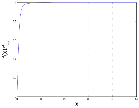
Figure 1: Plot of $f(x)/f_{\infty}$ as a function of $x$ for $v=1$, $\Lambda_{c}=-0.0671$.

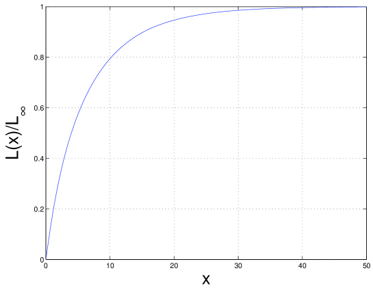
Figure 2: Plot of $L(x)/L_{\infty}$ as a function of $x$ for $v=1$, $\Lambda_{c}=-0.0671$.

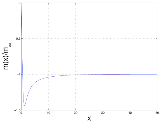
Figure 3: Plot of $m(x)/m_{\infty}$ as a function of $x$ for $v=1$, $\Lambda_{c}=-0.0671$.

In figure 1 we show the evolution of the scalar field, represented by $f(x)$ normalized to its value at infinity, which is given by $f_{\infty}=0.99577$, i.e. the field gets stabilized just before its minimum located at $v=1$. As for the two warp factors, $L(x)$ and $m(x)$, shown in figures 2 and 3 respectively, we can see how both go to constants at infinity. The associated geometry of the space-time is, therefore, that of a cigar, which goes to $AdS_{5}\times S_{1}$ asymptotically.

We have performed a systematic analysis of the parameter space, by varying the value of $v$ and adjusting the corresponding one of $\Lambda_{\rm c}$. The results are shown in figure 4, where we plot the warp factor $m(x)$ as a function of $x$ for $v=1.4,1,0.7,0.6$. As we can see, the smaller $v$ is the longer it takes the gravity fields to settle at their asymptotic values. This is just reflecting the fact that, for smaller $v$, the scalar field tends to settle closer and closer to its minimum, playing less of a role in the stabilization of the warp factors. In other words the problem becomes a typical two-scale one, where the scalar field quickly converges whereas the other two slowly flow to their asymptotic values. Therefore, the numerical involvement of the problem increases as we decrease the value of $v$.

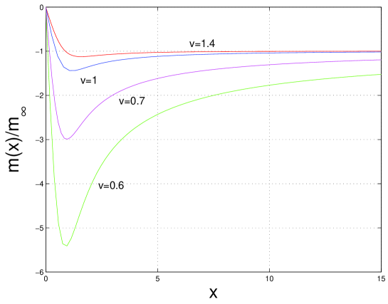
Figure 4: Plot of $m(x)/m_{\infty}$ as a function of $x$ for $v=1.4$, $v=1$, $v=0.7$ and $v=0.6$

To further comment on numerical issues, let us describe how difficult it is to obtain these solutions. As mentioned before, for a given model, there exists a regular solution just for a unique value of $\Lambda$. This was thoroughly explained in Ref. Gregory:1999gv , and here we shall merely repeat the main arguments and give a numerical proof. Essentially it is fair to study this system in its asymptotic region by assuming the scalar field $f(r)$ to be at its minimum and working with just the two warp factors $L(r)$ and $m(r)$. Then we can define the following variables

$$x = \frac{1}{-2\Lambda}\left(3m+\frac{L^{\prime}}{L}\right)\;\;,$$

$$y = \frac{1}{-2\Lambda}\frac{L^{\prime}}{L}\;\;,$$

which, together with the independent variable $\rho=x\sqrt{-2\Lambda}$, define the following autonomous dynamical system,

$$x^{\prime} = \frac{xy}{3}-\frac{4}{3}y^{2}\;\;,$$

$$y^{\prime} = \frac{4}{3}x(x-y)-y^{2}-\frac{3}{4}\;\;.$$

The primes here mean derivatives with respect to $\rho$.

In order to understand the structure of these numerical solutions, we must calculate the critical points of this system. Those are given by

$$c_{1}^{\pm} = \left(\pm\frac{3}{4},0\right)\hskip 142.26378pt{\rm saddle}$$

$$c_{2}^{\pm} = \pm\left(\sqrt{\frac{4}{5}},\frac{1}{\sqrt{4\times 5}}\right)\hskip 85.35826pt{\rm attractor}/{\rm repellor}$$

The solutions we have found, which we have shown in previous plots, correspond to flowing towards $c_{1}^{-}$ and it is now easy to understand why they are so hard to obtain: this is a saddle point, which is next to a repellor, given by $c_{2}^{-}$ (which, by the way, would be the critical point describing a geometry of the type $AdS_{6}$). Essentially only one trajectory, the one corresponding to $\Lambda_{\rm c}$, ends up in $c_{1}^{-}$ which can be matched to a regular solution near the core of the string. Solutions ending up in $c_{1}^{+}$ would correspond to a four dimensional metric that would blow-up.

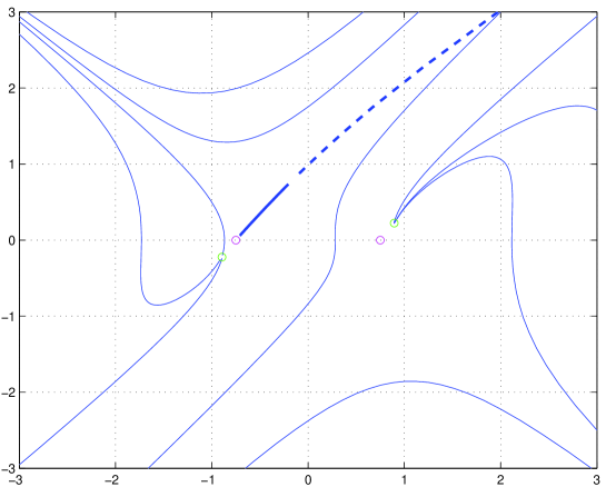
Figure 5: Plot of the $(x,y)$ phase space, for $v=1$.

For completeness we give a plot of the phase space for this autonomous system in figure 5, where we have also inserted the solution we have found (with a thick line). As we can see, far enough from the saddle point $c_{1}^{-}$, the scalar field $F(r)$ still plays a role in the evolution of $x$ and $y$ and, therefore, the inserted trajectory does not fit too well within those obtained from solving the system (LABEL:autu). We have highlighted this by using dashed lines in that part of our solution. As the field $F(r)$ plays less of a role, the trajectory starts to fit ’naturally’ into the phase space drawn, and that is represented by the continuous thick line.

In fact, one can even go further and obtain an analytic expression for the two warp factors $L(r)$ and $m(r)$ as they approach their asymptotic limit. This is done by rewriting the autonomous system Eq. (LABEL:autu) in the linear approximation around $c_{1}^{-}$, and solving for the two functions. The final result is that

$${\rm ln}\left(\frac{L(r)}{L_{\infty}}\right) = -A{\rm e}^{2(1-\sqrt{3})m_{\infty}r}\;\;,$$

$$\frac{m(r)}{m_{\infty}} = -\left(1-(1-2/\sqrt{3})A{\rm e}^{2(1-\sqrt{3})m_{\infty}r}\right)\;\;.$$

The $A$ factor, which determines the normalization of the curves, can then be extracted from our numerical results. We have checked that the results we get for $A$ from the two curves, i.e. $L(r)$ and $m(r)$, are compatible with each other and that the fit to both functions in the asymptotic region is extremely accurate.

Next, we would like to discuss the role played by the cosmological constant in the bulk, $\Lambda$. As it was mentioned at the beginning of this section, we have numerically checked that, for every value of $v$ there is a unique value of $\Lambda$, which we denote as $\Lambda_{c}$, that gives us a regular solution everywhere. We have explored the parameter space defined by $\Lambda_{c}/\lambda$ and $v$, and we have compared our results with existing ones in the literature.

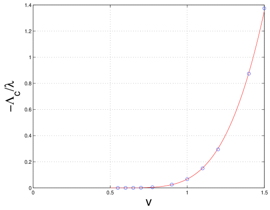
Figure 6: Plot of $-\Lambda_{c}/\lambda$ as a function of $v$, for small values of the latter. We have superimposed to the data the best fit we could find, given by eq. (21) with $a=6.3$, $b=9.0$.

For small values of $v$, see figure 6, we find a very good linear fit to the quantity $v{\rm log}(-\Lambda_{c}/\lambda)$, which means that, in that region

$$\frac{\Lambda_{c}}{\lambda}=-{\rm e}^{a-b/v}\;\;.$$ (21)

We have compared these results to the estimate given in Ref. Gregory:1999gv , i.e. $\Lambda\sim\epsilon{\rm e}^{-1/\epsilon}$, where $\epsilon=v^{2}$. This estimate was made for very small values of $v$ and assuming the constraint $\lambda v^{2}=1$. Taking these facts into account, we find remarkable similarity between that result and the numbers we obtain as, in our language, that estimate reads $\Lambda_{c}/\lambda\sim{\rm e}^{-1/v^{2}}$, to be compared to eq. (21). However, as mentioned above, numerical difficulties prevent us from exploring the region of very small $v$ and, therefore, we cannot check the validity of this equation in that region.

Having already mentioned the numerical difficulties encountered when exploring the small $v$ region, which corresponds to the weak gravity limit, we turned to explore large values for $v$. As it happens, there is an upper bound on the value of $\Lambda_{c}$ if we want to obtain regular solutions that trap gravity. This is given by the quantity $m_{1}/v^{2}$ vanishing, or, in other words, by

$$1+\frac{\Lambda_{c}}{\lambda v^{4}}\rightarrow 0\;\;.$$ (22)

We show this graphically in figure 7, where we plot $-\Lambda_{c}/(\lambda v^{4})$ as a function of $v$, indicating the points that were calculated numerically. We can clearly see that we are approaching the super heavy limit, given by eq. (22), and we can calculate how the different relevant quantities in our problem approach it. For example, the asymptotic value of the scalar field, $f_{\infty}$, using eq. (15), will be given by

$$f_{\infty}^{sh}=\sqrt{\frac{6}{7}}v\;\;,$$ (23)

which means that, in the limit where gravity is strongest, the field will be maximally displaced from the minimum of its potential, at a value given by

$$V(f_{\infty}^{sh})=\lambda\frac{v^{4}}{49}\;\;.$$ (24)

The other two asymptotic quantities will be given by

$$m_{\infty}^{sh} = \pm\sqrt{6\lambda}\frac{v^{2}}{7M_{6}^{2}}$$

$$L_{\infty}^{sh} = \frac{\sqrt{7}}{2}\frac{1}{\sqrt{\lambda}v}\;\;.$$

Note that, in terms of adimensional quantities, $m_{\infty}^{sh}=\sqrt{6}v/(7M_{6}^{2})$, and $L_{\infty}^{sh}=\sqrt{7}/2$.

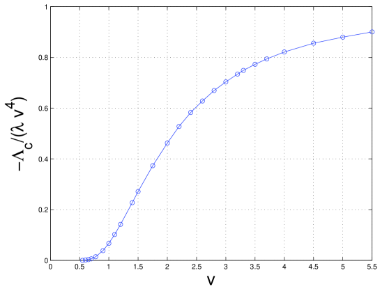
Figure 7: Plot of $-\Lambda_{c}/(\lambda v^{4})$ as a function of $v$.

Finally, we should comment on the phenomenological applications of our results. One of the motivations to study these kind of set-ups is to try to generate a large hierarchy between the higher dimensional and the $D=4$ Planck masses in order to explain the so-called hierarchy problem of traditional grand unified theories. Here these two scales are related by the following equation

$$M_{\rm Planck}^{2}=\frac{2\pi M_{6}^{4}}{\lambda v^{2}}\int dxM^{2}(x)L(x)\;\;,$$ (26)

where, as explained after eq. (11), $m(x)=M^{\prime}(x)/M(x)$. We have checked that, in the solutions we have found, the hierarchy is never larger than a few orders of magnitude (order $100$ for $v=1$, increasing to order $1000$ for $v=0.7$), and obtaining a $D=6$ scale of the order of the TeV proves numerically unachievable. It would correspond to a region with very small $v$, as already pointed out in Ref. Gregory:1999gv , which we cannot access given that, as mentioned before, our problem turns into a two-scale one, and our numerical tools become insufficient.

IV Discussion and Conclusions

There are in the literature several confining gravity solutions that involve scalar vortices in six dimensions Gherghetta:2000qi ; Giovannini:2001hh ; deCarlos:2003nq . In particular, complete numerical solutions have been presented in two cases Giovannini:2001hh ; deCarlos:2003nq . It is interesting to compare our work with these solutions.

In the first one, Ref. Giovannini:2001hh , Giovannini et al. studied a general gravity trapping abelian vortex. The presence of the gauge field is crucial and determines the properties of the solution. It is described by three parameters, $\Lambda$, $v$, and a new one, $\alpha$, that fixes the gauge coupling. The authors find that the condition of gravity trapping translates into a fine tuning among these three parameters, fixing a critical surface in this space. The corresponding metric, that is a solution to the field equations, exhibits both Minkowski and angular warp factors that decrease when $r$ increases. This has to be compared to our case, where only the Minkowski factor decreases since the solution is cigar-like. This fine tuning is a generic fact in this kind of models, and appears when we try to connect the required behaviours for the metric: a regular one at the origin and a confining one for large values of $r$. The presence of the gauge field does not change this fact.

In the second one, Ref. deCarlos:2003nq , a cigar-like solution based on a BPS scalar vortex was studied. The potential was derived from a Supergravity (SUGRA) like theory and its structure was almost fixed. In particular, there was no room for a cosmological constant. Nevertheless, this SUGRA inspired potential is negative near the local minimum, acting like a negative cosmological constant for values of the scalar field close to it. The choice of the potential was dictated by simplicity, since for that specific form the field equations are first order (for more details see Ref. Carroll:1999mu ). Therefore numerical solutions are easily obtained just by integrating these first order equations together with regular boundary conditions at the origin, which happen to be gravity trapping. The SUGRA like structure induces the connection of the two (origin and large $r$) required metric behaviours in the solution. Notice that there is an implicit fine tuning in the model in the choice of the potential. If we slightly change the coefficients of the terms appearing in the potential, the new model will almost certainly not admit a confining solution. This is related to the stability of the solution against radiative corrections, which is an issue is beyond the scope of our work.

To conclude, in this paper we have analyzed the global string in a six-dimensional space time with a negative bulk cosmological constant, $\Lambda$. We have presented numerical evidence of the existence of solutions that confine gravity. For every value of $v$, the Higgs vev, there is unique value of $\Lambda$ that provides a regular solution. This critical cosmological constant is bounded by $-V(0)<\Lambda_{c}<0$ and approaches its lowest value in the strong gravity limit. On the other hand, it is difficult to get a hierarchy between $M_{6}$ and $M_{Planck}$, at least in the range we have been able to explore numerically.

- (1) K. Akama, “An Early Proposal Of ’Brane World’,” Lect. Notes Phys. 176, 267 (1982), [arXiv:hep-th/0001113].
- (2) V. A. Rubakov and M. E. Shaposhnikov, “Extra Space-Time Dimensions: Towards A Solution To The Cosmological Constant Problem,” Phys. Lett. B 125, 139 (1983).
- (3) M. Visser, “An Exotic Class Of Kaluza-Klein Models,” Phys. Lett. B 159 (1985) 22 [arXiv:hep-th/9910093].
- (4) A. Vilenkin, “Gravitational Field Of Vacuum Domain Walls,” Phys. Lett. B 133, 177 (1983).
- (5) J. Ipser and P. Sikivie, “The Gravitationally Repulsive Domain Wall,” Phys. Rev. D 30, 712 (1984).
- (6) M. Cvetic and H. H. Soleng, “Supergravity domain walls,” Phys. Rept. 282, 159 (1997) [arXiv:hep-th/9604090].
- (7) G. W. Gibbons, “Global Structure Of Supergravity Domain Wall Space-Times,” Nucl. Phys. B 394, 3 (1993).
- (8) M. Cvetic, S. Griffies and H. H. Soleng, “Local and global gravitational aspects of domain wall space-times,” Phys. Rev. D 48, 2613 (1993) [arXiv:gr-qc/9306005].
- (9) F. Bonjour, C. Charmousis and R. Gregory, “Thick domain wall universes,” Class. Quant. Grav. 16, 2427 (1999) [arXiv:gr-qc/9902081].
- (10) M. Barriola and A. Vilenkin, “Gravitational Field Of A Global Monopole,” Phys. Rev. Lett. 63, 341 (1989).
- (11) A. G. Cohen and D. B. Kaplan, “The Exact Metric About Global Cosmic Strings,” Phys. Lett. B 215, 67 (1988).
- (12) R. Gregory, “Non-singular global strings,” Phys. Rev. D 54, 4955 (1996) [arXiv:gr-qc/9606002].
- (13) L. Randall and R. Sundrum, “A large mass hierarchy from a small extra dimension,” Phys. Rev. Lett. 83, 3370 (1999) [arXiv:hep-ph/9905221].
- (14) I. Olasagasti and A. Vilenkin, “Gravity of higher-dimensional global defects,” Phys. Rev. D 62, 044014 (2000) [arXiv:hep-th/0003300].
- (15) A. G. Cohen and D. B. Kaplan, “Solving the hierarchy problem with noncompact extra dimensions,” Phys. Lett. B 470, 52 (1999) [arXiv:hep-th/9910132].
- (16) R. Gregory, “Nonsingular global string compactifications,” Phys. Rev. Lett. 84, 2564 (2000) [arXiv:hep-th/9911015].
- (17) R. Gregory and C. Santos, “Spacetime structure of the global vortex,” Class. Quant. Grav. 20, 21 (2003) [arXiv:hep-th/0208037].
- (18) T. Gherghetta and M. E. Shaposhnikov, “Localizing gravity on a string-like defect in six dimensions,” Phys. Rev. Lett. 85, 240 (2000) [arXiv:hep-th/0004014]; A. Chodos and E. Poppitz, “Warp factors and extended sources in two transverse dimensions,” Phys. Lett. B 471, 119 (1999) [arXiv:hep-th/9909199]; E. Ponton and E. Poppitz, “Gravity localization on string-like defects in codimension two and the AdS/CFT correspondence,” JHEP 0102, 042 (2001) [arXiv:hep-th/0012033].
- (19) M. Giovannini, H. Meyer and M. E. Shaposhnikov, “Warped compactification on Abelian vortex in six dimensions,” Nucl. Phys. B 619, 615 (2001) [arXiv:hep-th/0104118].
- (20) B. de Carlos and J. M. Moreno, “A cigar-like universe,” JHEP 0311 (2003) 040 [arXiv:hep-th/0309259].
- (21) S. M. Carroll, S. Hellerman and M. Trodden, “BPS domain wall junctions in infinitely large extra dimensions,” Phys. Rev. D 62 (2000) 044049 [arXiv:hep-th/9911083].