Soft Supersymmetry Breaking on the Brane

Abstract

We consider the low energy description of five dimensional models of supergravity with boundaries comprising a vector multiplet and the universal hypermultiplet in the bulk. We analyse the spontaneous breaking of supersymmetry induced by the vacuum expectation value of superpotentials on the boundary branes. When supersymmetry is broken, the moduli corresponding to the radion, the zero mode of the vector multiplet scalar field and the dilaton develop a potential in the effective action. We compute the resulting soft breaking terms and give some indications on the features of the corresponding particle spectrum. We consider some of the possible phenomenological implications when supersymmetry is broken on the hidden brane.

I Introduction

Supersymmetry breaking is one of the unsolved challenges of particle physics. A proper understanding of the origin of supersymmetry breaking would certainly increase the prospects of an experimental discovery of supersymmetry and shed new light on thorny issues such as the cosmological constant problem. Many models of supersymmetry breaking have been proposed so far. Amongst the most popular are the gravity mediated and gauge mediated scenarios (see gravity_gauge_mediated for reviews). Each have interesting features although none provide a completely satisfactory framework. Recently brane models have been introduced and address both the hierarchy problem ADD ; RS1 and the cosmological constant problem selftuning . Brane models have been originally built up in a non-supersymmetric setting. The supersymmetrisation of the Randall-Sundrum model Altendorfer:2000rr ; Falkowski:2000er and models with a bulk scalar field kallosh ; offshell ; flp2 provide a justification for certain fine–tunings used in brane models in order to find flat brane solutions. Later it has been noticed that supersymmetry is in fact compatible with branes of lower tension than the Randall-Sundrum case Brax:2001xf ; susyRS_arbitrary_tensions ; Brax:2002vs ; Lalak:2002kx ; twisted_sugra ; twist_warp_sugra . When the tensions are detuned, the 5d action of the theory is supersymmetric, but can be built so that the warped background solutions of the equations of motion either break supersymmetry or not. Hence this may realize a spontaneous breaking of supersymmetry in five dimensions. Other types of supersymmetry breaking solutions with tension detuning, which do not correspond to static warped backgrounds with straight branes, can lead to strongly 4d Lorentz violating effects kinetic_susy_breaking ; detuned .

At sufficiently low energy, well below the brane tensions, supersymmetric brane models can be described by a 4d supersymmetric effective action luty1 ; susy_radion ; flp3 ; effective_detuned ; effective_sugra . This 4d effective action is determined by a Kähler potential for the moduli fields. When the bulk contains a vector multiplet and the universal hypermultiplet, the moduli describe the radion, the zero mode of the vector multiplet scalar field and the dilaton, i.e. the zero mode of the hypermultiplet. The moduli coming from the vector multiplet bulk scalars are associated to the axion–like fields originating from the fifth components of the bulk vector fields. The existence of these massless moduli may imply strong deviations from general relativity testsGR . The cosmology of these tensor–scalar theories is also interesting rev1 ; rev2 and may be probed using the CMB anisotropies cosmoduli ; CMB .

The supersymmetric low energy action in the Randall-Sundrum case has been nicely spelt out in effective_detuned . Detuning the brane tensions by including constant superpotentials leads to an effective potential for the radion. It corresponds to the fact that the detuned boundary conditions are no longer compatible with 4d Poincaré supersymmetry . The brane system is then subject to a back-reaction effect which can be analysed using the equations of motion of the low-energy action. When the radion effective potential admits a minimum, this value of the radion is equal to the one obtained by solving the 5d equations with detuned tensions. At the minimum, the potential is negative and supersymmetry is preserved for specific values of the radion imaginary part, as the F–terms of the radion vanishes, corresponding to $AdS_{4}$ supergravity. This is the same result as obtained analysing the 5d equations of motion and Killing spinor equations. Notice that the resulting configuration breaks Poincaré invariance.

In the present article, we study the low energy action of brane models with bulk scalar fields belonging to a vector multiplet and the universal hypermultiplet of 5d $N=2$ supergravity. We include the effects of a detuning of the brane tensions in the form of superpotentials on the branes. Supersymmetry is then broken by the $F$–terms associated to the moduli. We analyse both the cosmological and the particle physics consequences of such a breaking.

Our analysis of the breaking of supersymmetry extends to the case with a vector multiplet the results of flp3 where the Randall–Sundrum model with a hypermultiplet in the bulk was considered. The phenomenology of this model has been spelt out in casas with particular emphasis on the electro–weak symmetry breaking, for matter on the negative tension brane and specific assumptions about moduli stabilisation. On the contrary, we consider the case where matter lives on the positive tension brane with no assumption about moduli stabilisation. We envisage the case when moduli may not be stabilised and take into account the corresponding solar system constraints.

A particular stumbling block of supersymmetric models is the origin of the hierarchy between a large scale such as the Planck mass and the $\mu$ term. In the following we will show that when a $\mu$ term is included on the positive tension brane, a large hierarchy can be induced thanks to the presence of the vector multiplet scalar field in the bulk. Similarly, when supersymmetry is broken on the hidden brane of negative tension, and no $\mu$ term is included in the superpotential of the positive tension brane, an effective $\mu$ term results from anomaly mediation.

Breaking supersymmetry using boundary superpotentials has been investigated in luty2 ; zwirner in the flat case where the brane tensions vanish. In the flat case, a $N=1$ superspace formulation of $D=5$ supergravity coupled to boundary branes has been elaborated in phil1 and used to compute quantum corrections to the soft breaking terms phil2 . In the case that we consider, the bulk background is warped. We analyse the non–trivial effects induced by such a warping on the breaking of supersymmetry. In particular all our results apply to the Randall–Sundrum setting where matter lives on the positive tension brane.

When supersymmetry is broken on the hidden brane of negative tension and matter lives on the positive tension brane, we find that soft supersymmetry breaking terms are of two sorts. First of all the soft trilinear $A$ terms and the gaugino masses receive a non–vanishing contribution at one–loop level from anomaly mediation. Secondly and contrarily to anomaly mediation scenarios, the soft masses are non-vanishing at tree level. Therefore they do not suffer from the tachyons of anomaly mediated models.

In section 2 we present the models including a bulk vector multiplet and study the zero–modes, i.e. we give different parametrisations of the low energy moduli. In section 3 we analyse the low energy action computing the Kähler potential and the superpotential when coupling 5d supergravity with a vector multiplet in the bulk to matter on the branes. We also discuss the dilaton arising from the bulk hypermultiplet. In section 4 we focus on the case with no hypermultiplet and compute both the moduli potential and the soft breaking terms at the classical level. We then introduce the dilaton field in section 5 and discuss race–track models. In section 6, we discuss the one–loop anomaly mediated soft terms. In section 7, we focus on supersymmetry breaking on the hidden brane, making explicit the soft breaking terms and the associated phenomenology. In section 8, we introduce an explicitly supersymmetry breaking step by taking into account charges on the branes in order to bypass the cosmological constant problem. This leads to an extra contribution to the moduli potential. Finally in section 9, we discuss the cosmological consequences and the gravitational constraints on the models. We also include two appendices. In a first appendix, we discuss the Randall-Sundrum case and radion stabilisation. In the second one, we give the Randall-Sundrum soft terms.

II Supergravity with Boundary Branes

II.1 Supergravity Construction

For the bulk theory with no brane coupling, ${\mathcal{N}}=2$ $D=5$ pure supergravity was first constructed in 5d pure sugra  ; vector multiplets were added in vector coupling , and finally vector multiplets, hypermultiplets and tensor multiplets were treated together in vector-tensor-hyper . Gauged supergravity with boundary branes in five dimensions has been elegantly constructed when vector multiplets live in the bulk kallosh ; offshell . The supergravity multiplet comprises the metric tensor $g_{ab}$, $a,b=1\dots 5$, the gravitini $\psi_{a}^{A}$ where $A=1,2$ is an $SU(2)_{R}$ index and the graviphoton field $A_{a}$. The ${\mathcal{N}}$=2 vector multiplets in the bulk possess one vector field, a $SU(2)_{R}$ doublet of symplectic Majorana spinors and one real scalar. When considering $n$ vectors multiplets, it is convenient to denote by $A^{I}_{a}$, $I=1\dots n+1$, the $(n+1)$ vector fields.

The two boundaries are fixed points of a $Z_{2}$ orbifold like in the Randall-Sundrum model and its supersymmetrisation. The action on each brane depends on two ingredients. First the branes couple to the bulk, i.e. to gravity and the real scalar fields. Then ordinary matter is confined to either of the branes. In the following, we will first describe the bulk and brane theory without matter.

The supergravity theory with boundaries differs from usual five-dimensional non supersymmetric theories with boundaries as new superpartner fields are introduced in order to close the supersymmetry algebra and ensure the invariance of the Lagrangian. The vector multiplets comprise scalar fields $\phi^{i}$ parameterizing the manifold

$$C_{IJK}h^{I}(\phi)h^{J}(\phi)h^{K}(\phi)=1$$ (1)

with the functions $h^{I}(\phi),I=1\dots n+1$ playing the role of auxiliary variables. In heterotic M–theory ovrut the symmetric tensor $C_{IJK}$ has the meaning of an intersection tensor. Defining the metric

$$G_{IJ}=-2C_{IJK}h^{K}+3h_{I}h_{J}$$ (2)

where $h_{I}=C_{IJK}h^{J}h^{K}$, the bosonic part of the Lagrangian (vector fields not included) reads

$$S_{bulk}=\frac{1}{2\kappa_{5}^{2}}\int d^{5}x\sqrt{-g_{5}}\Big{(}{\mathcal{R}}-\frac{3}{4}(g_{ij}\partial_{\mu}\phi^{i}\partial^{\mu}\phi^{j}+V)\Big{)}$$ (3)

where the sigma-model metric $g_{ij}$ is

$$g_{ij}=2G_{IJ}\frac{\partial h^{I}}{\partial\phi^{i}}\frac{\partial h^{J}}{\partial\phi^{j}}$$ (4)

and the potential is given by

$$V=U_{i}U^{i}-U^{2}$$ (5)

using the sigma-model metric $g_{ij}$. The superpotential $U$ defines the dynamics of the theory. It is given by

$$U=4\sqrt{\frac{2}{3}}gh^{I}V_{I}$$ (6)

where $g$ is a gauge coupling constant and the $V_{I}$’s are real numbers such that the $U(1)$ gauge field is $A^{I}_{a}V_{I}$.

The boundary action depends on two new fields. There is a supersymmetry singlet $G$ and a four form $A_{\mu\nu\rho\sigma}$ kallosh . One also modifies the bulk action by replacing $g\to G$ and adding a direct coupling

$$S_{A}=\frac{2}{4!\kappa_{5}^{2}}\int d^{5}x\epsilon^{abcde}A_{abcd}\partial_{e}G.$$ (7)

The boundary action is taken as

$$S_{bound}=-\frac{1}{\kappa_{5}^{2}}\int d^{5}x(\delta_{x_{5}}-\delta_{x_{5}-R})(\sqrt{-g_{4}}\frac{3}{2}U+\frac{2g}{4!}\epsilon^{\mu\nu\rho\sigma}A_{\mu\nu\rho\sigma}).$$ (8)

where $\mu,\nu,\rho,\sigma$ are four-dimensional indices on the branes. Notice that the four-form $A_{abcd}$ is not dynamical. According to this action the branes can be seen as charged under this bulk four-form with a charge $\pm g$. In section VIII we will consider branes charged under a new bulk four-form with kinetic terms and arbitrary charge, in order to cancel the vacuum energy.

The supersymmetry algebra closes on shell where

$$G(x)=g\epsilon(x_{5}),$$ (9)

and $\epsilon(x_{5})$ jumps from -1 to 1 at the origin of the fifth dimension. On shell the bosonic Lagrangian reduces to the bulk Lagrangian coupled to the boundaries as,

$$S_{bound}=-\frac{3}{2\kappa_{5}^{2}}\int d^{5}x(\delta_{x_{5}}-\delta_{x_{5}-R})\sqrt{-g_{4}}U,$$ (10)

Crucially, the boundary branes couple directly to the bulk superpotential. Notice that the two branes have opposite (field-dependent) tensions

$$\lambda_{\pm}=\pm\frac{3}{2\kappa_{5}^{2}}U$$ (11)

where the first brane has positive tension.

Let us focus on the case of a single vector multiplet $n=1$. The equations of motion can be written in a first order BPS form

$$\frac{a^{\prime}}{a}=-\frac{U}{4},\ \phi^{\prime}=\frac{\partial U}{\partial\phi},$$ (12)

where ${}^{\prime}=d/dz$ for a metric of the form

$$ds^{2}=dz^{2}+a^{2}(z)\eta_{\mu\nu}dx^{\mu}dx^{\nu}.$$ (13)

The boundary conditions are automatically satisfied implying that the positions of the two boundary branes are not specified. Moreover the BPS background preserves $N=1$ Poincaré supersymmetry from the four dimensional point of view. Indeed denote by $\epsilon^{A}$ the supersymmetry parameter of $N=2$ 5d supergravity. The Killing spinor solutions of $\delta_{\epsilon}\psi_{a}^{A}=0$ satisfy kallosh

$$\epsilon^{A}(z,x^{\mu})=a^{1/2}(z)\epsilon^{A}$$ (14)

where $\epsilon^{A}$ is a constant spinor such that $\gamma_{5}\epsilon^{A}=(\sigma_{3})^{A}_{B}\epsilon^{B}$ implying that only one chirality of the original supersymmetries is preserved. Having obtained Killing spinors corresponding to $N=1$ 4d supersymmetry, we will explicitly find that the low energy Lagrangian can be written in a 4d supersymmetric way.

Let us give the simplest example of models of supergravity with a single scalar field BD . We choose only one vector multiplet and the only component for the symmetric tensor $C_{IJK}$ is $C_{122}=1$. The moduli space of vector multiplets is then defined by the algebraic relation

$$3h^{1}(h^{2})^{2}=1.$$ (15)

This allows to parameterize this manifold using the coordinate $\phi$ such that $h^{1}$ is proportional to $e^{\sqrt{\frac{1}{3}}\phi}$ and $h^{2}$ to $e^{-\phi/2\sqrt{3}}$. The induced metric $g_{\phi\phi}$ can be seen to be one. The most general superpotential is a linear combination of the two exponentials $U=ae^{\sqrt{\frac{1}{3}}\phi}+be^{-\phi/2\sqrt{3}}$. In the following we will focus on models where the superpotential $U$ can be expressed as an exponential of the normalised scalar field $\phi$

$$U=4ke^{\alpha\phi}.$$ (16)

The values $\alpha=1/\sqrt{3},-1/\sqrt{12}$ correspond to the previous example. The metric in the bulk depends on the scale factor

$$a(z)=(1-4k\alpha^{2}z)^{\frac{1}{4\alpha^{2}}},$$ (17)

while the scalar field solution is

$$\phi=-\frac{1}{\alpha}\ln\left(1-4k\alpha^{2}z\right).$$ (18)

In the $\alpha\to 0$ we retrieve the AdS profile

$$a(z)=e^{-kz}.$$ (19)

corresponding to the supersymmetric Randall-Sundrum model with no vector multiplet in the bulk.

II.2 The zero–modes

The BPS configurations have zero modes solving the linearised equations of motion together with the boundary conditions at the branes. The linearised Einstein and Klein–Gordon equations have been thoroughly studied in chris1 following an earlier work christos in the Randall–Sundrum case. The end result is that there are two scalar modes and one spin two mode. They correspond to either the radion and the zero mode of the bulk scalar field or the two brane positions. The spin two zero mode, i.e. the graviton, is associated to 4d gravity at low energy.

The number of moduli can be inferred by a counting argument based on supersymmetry. At low energy, the only imprint of the two bulk vector fields $A_{a}^{I},\ I=1,2,$ are two pseudo–scalar fields $A_{5}^{I}$ (the vector fields are projected out by the $Z_{2}$ symmetry). These two axion–like fields are combined with the radion and the bulk scalar field to form the scalar fields comprising two chiral superfields. Already in the Randall–Sundrum case, the radion can be seen as the fluctuation of the $g_{55}$ component of the bulk metric and is associated to the zero mode of the gravi–photon $A_{5}$. This remains true and is complemented by the association of the bulk scalar field zero mode of the vector multiplet to the corresponding axion–like field in the vector multiplet.

The two scalar zero modes can be viewed as the two brane positions

$$t_{1}=\xi_{1}(x),\ t_{2}=r+\xi_{2}(x)$$ (20)

representing the massless fluctuations with respect to fixed branes at $0$ and $r$

$$\Box^{(4)}\xi_{1,2}=0$$ (21)

where the bulk metric is unperturbed.

Equivalently the two branes can be considered as fixed and the metric is perturbed

$$ds^{2}=a^{2}(G(x,z))g_{\mu\nu}dx^{\mu}dx^{\nu}+(\partial_{z}G)^{2}dz^{2}$$ (22)

where $g_{\mu\nu}=\eta_{\mu\nu}+h_{\mu\nu}$ is the perturbed 4d metric and

$$G(x,z)=z+\frac{\xi(x)}{a^{2}(z)}+\xi_{0}(x)$$ (23)

where

$$\Box^{(4)}\xi=0,\ \Box^{(4)}\xi_{0}=0$$ (24)

and

$$\xi_{1}=\frac{\xi}{a_{1}^{2}}+\xi_{0},\ \xi_{2}=\frac{\xi}{a_{2}^{2}}+\xi_{0}$$ (25)

The radion is related to $\xi$ as

$$t(x)=(\frac{1}{a_{2}^{2}}-\frac{1}{a_{1}^{2}})\xi(x)$$ (26)

where $a_{1,2}$ are the scale factors of the first and second branes. The mode $\xi_{0}$ is associated to a global translation of the bulk–brane system. Similarly the scalar field is perturbed as

$$\phi(x,z)=\phi_{BPS}(G(x,z))$$ (27)

No intrinsic zero–mode is associated to the scalar field.

To linear order, this parametrisation is equivalent to

$$\delta g_{55}=-2\frac{a^{\prime}}{a^{3}}\xi$$ (28)

confirming the link between $\delta g_{55}$ and the radion. Similarly the perturbed scalar field is

$$\frac{\delta\phi}{\phi^{\prime}_{BPS}}=2\frac{\delta g_{55}}{U}+\frac{\partial U}{\partial\phi}\xi_{0}$$ (29)

picking contributions from $\delta g_{55}$ and $\xi_{0}$.

Finally, one can also use a parametrisation generalising the one of effective_detuned

$$ds^{2}=A^{2}(x,z)\Omega^{2}(x,z)g_{\mu\nu}dx^{\mu}dx^{\nu}+\frac{(a^{2}+2aa^{\prime}\xi_{0})^{2}}{A^{4}}dz^{2}$$ (30)

where

$$A^{2}=a^{2}+2\frac{a^{\prime}}{a}\xi+2aa^{\prime}\xi_{0}$$ (31)

and

$$\Omega^{2}=(1-\frac{a_{1}^{2}-a_{2}^{2}}{\int_{0}^{r}a^{2}dz}\xi_{0})^{-1}$$ (32)

The dimensional reduction using this ansatz leads to an action in the Einstein frame for the two moduli $\xi_{0}$ and $\xi$.

In the following, we will work exclusively with the two moduli $t_{1,2}$ as the parametrisation is simpler.

III The Low Energy Action

III.1 The vector multiplet sector

At low energy the brane and bulk system is amenable to a four–dimensional treatment where the dynamics are captured by the slow motion of moduli fields. Two of the moduli of the system are the brane positions as they are not specified by the equations of motions. At low energy, one considers small deformations of the static configuration allowing the moduli to be space–time dependent. We denote the position of brane 1 by $t_{1}(x^{\mu})$ and the position of brane 2 by $t_{2}(x^{\mu})$. We consider the case where the evolution of the brane is slow. This means that in constructing the effective four–dimensional theory we neglect terms of order higher than two in a derivative expansion. Moreover the non-linearity of the Einstein equations on the branes in the matter energy–momentum tensors project are neglected. Such a regime is only valid at low energy well below the brane tensions of both branes. For instance, putting the standard model matter on the positive tension brane leads to an effective action valid only up to the positive brane tension. In addition to the brane positions, we need to include the graviton zero mode, which can be done by replacing $\eta_{\mu\nu}$ with a space–time dependent tensor $g_{\mu\nu}(x^{\mu})$.

After integrating over the fifth dimension, one obtains a 4d effective action. The Einstein-Hilbert term in 4d follows from the 5d term and reads

$$S_{\rm bulk}=\int d^{4}x\sqrt{-g_{4}}f(t_{1},t_{2}){\cal R}^{(4)},$$ (33)

with

$$f(t_{1},t_{2})=\frac{1}{\kappa_{5}^{2}}\int^{t_{2}}_{t_{1}}dza^{2}(z)$$ (34)

For the exponential superpotential $U$, this is

$$f(t_{1},t_{2})=\frac{a(t_{1})^{2+4\alpha^{2}}-a(t_{2})^{2+4\alpha^{2}}}{(2+4\alpha^{2})k\kappa_{5}^{2}}.$$ (35)

Notice that the action is in the brane frame different from the Einstein frame. Including the boundary terms leads to the following effective action cosmoduli

$$S=\int d^{4}x\sqrt{-g_{4}}\left[f(t_{1},t_{2}){\cal R}^{(4)}+\frac{3}{4}a^{2}(t_{1})\frac{U(t_{1})}{\kappa_{5}^{2}}(\partial t_{1})^{2}-\frac{3}{4}a^{2}(t_{2})\frac{U(t_{2})}{\kappa_{5}^{2}}(\partial t_{2})^{2}\right].$$ (36)

As expected the moduli are free scalar fields.

The effective action for the two moduli $t_{1}$ and $t_{2}$ is written in an explicit supergravity form. This follows from the fact that the two-brane system satisfies BPS conditions. At low energy the bulk and brane system preserves one of the original supersymmetries. Indeed one can write the Einstein-Hilbert term and the kinetic terms of the moduli as

$$\int d^{4}x\sqrt{-g_{4}}\left[f(t_{1},t_{2}){\cal R}^{(4)}+6\partial_{T_{1}}\partial_{\bar{T}_{1}}f\partial_{\mu}T_{1}\partial^{\mu}\bar{T}_{1}+6\partial_{T_{2}}\partial_{\bar{T}_{2}}f\partial_{\mu}T_{2}\partial^{\mu}\bar{T}_{2}\right],$$ (37)

where

$$t_{1}=\frac{1}{2}(T_{1}+\bar{T}_{1}),\ t_{2}=\frac{1}{2}(T_{2}+\bar{T}_{2}).$$ (38)

This allows us to identify the fields $T_{1}$ and $T_{2}$ as the scalar parts of two chiral multiplets whose dynamics are captured by the function $f(t_{1},t_{2})$

$$\int d^{4}xd^{4}\theta E^{-1}f(\frac{T_{1}+\bar{T}_{1}}{2}\ ,\frac{T_{2}+\bar{T}_{2}}{2})$$ (39)

where $E$ is the vielbein determinant superfield. From this action one can read off the Kähler potential for the two moduli fields in the Einstein frame

$$K=-3\ln(\kappa_{4}^{2}f).$$ (40)

which depends on the two moduli. Notice that the Kähler potential possesses two global symmetries

$$T_{i}\to T_{i}+ib_{i}.$$ (41)

coming from the independence of the background geometry on the axion fields. A detailed analysis of the Kähler geometry with an arbitrary number of vector multiplets is under study kahler .

Let us now concentrate on the Randall–Sundrum case $\alpha=0$, the Kähler potential reads

$$K=-3\ln(e^{-k(T_{1}+\bar{T}_{1})}-e^{-k(T_{2}+\bar{T}_{2})}).$$ (42)

The Kähler potential can be written as

$$K=3k(T_{1}+\bar{T}_{1})-3\ln(1-e^{-k(T+\bar{T})}),$$ (43)

where

$$T=T_{2}-T_{1}$$ (44)

is the radion superfield. In the Randall–Sundrum case, the field $T_{1}$ can be eliminated by a Kähler transformation; this shows that one of the two moduli decouples, leaving only the radion as the relevant physical field.

III.2 The hypermultiplet sector

We can now introduce another ingredient, i.e. a hypermultiplet living in the bulk. We will focus on the universal hypermultiplet comprising four scalar fields, two being odd under the orbifold parity flp2 . We also assume that the hypermultiplet is not charged under the gauged $U(1)_{R}$ symmetry in such a way that no contribution from the hypermultiplet appears in the bulk potential. At low energy, the two even scalar fields become the scalar part of a chiral multiplet $S$ which will be called the dilaton in the following. The low energy dynamics of the dilaton is determined by the Kähler potential

$$K(S,\bar{S})=-\ln(S+\bar{S})$$ (45)

Notice that the full moduli Kähler potential is then just the sum of the vector multiplet and hypermultiplet contributions.

III.3 The coupling to matter

Let us now introduce matter on the boundary branes. We couple the matter fields to the induced metric on the ith–brane leading to an action for the matter scalar field $s$ coupled to the brane position $t_{i}$

$$\int d^{4}x\sqrt{-g}\Big{(}a^{2}(t)(\partial s\partial\bar{s})+a^{4}(t)|\frac{\partial w(s)}{\partial s}|^{2}\Big{)}$$ (46)

up to derivative terms in $t_{i}$. We have denoted by $w$ the superpotential of the supersymmetric theory on the brane. As we are supersymmetrising the matter action only at zeroth order in $\kappa_{4}$, we have suppressed the non-renormalizable terms in the matter fields for fixed moduli, hence the globally supersymmetric form of the potential. Such an action can be supersymmetrised (we follow the conventions of weinberg for the definitions of the Kähler potentials)

$$-3\int d^{4}xd^{4}\theta E^{-1}\Big{(}f-a^{2}(\frac{T_{i}+\bar{T}_{i}}{2})\Sigma\bar{\Sigma}\Big{)}$$ (47)

modifying the Kähler potential of the moduli

$$K=-3\ln(\kappa_{4}^{2}f-\frac{1}{3}\kappa_{4}^{2}a^{2}(\frac{T_{i}+\bar{T}_{i}}{2})\Sigma\bar{\Sigma})$$ (48)

where $\Sigma=s+\dots$ is the chiral superfield of matter on the brane (not to be confused with the hypermultiplet superfield S). Similarly the potential on the brane follows from

$$\int d^{4}xd^{2}\theta\Phi^{3}W(T_{i},S,\Sigma)$$ (49)

where

$$W(T_{i},S)=a^{3}(T_{i})w(S,\Sigma)$$ (50)

and $\Phi$ is the chiral compensator whose $F$–term is the gravitational auxiliary field. At low energy this leads to a direct coupling between matter fields and the moduli. This is crucial when discussing supersymmetry breaking. Moreover the coupling to the brane breaks the global symmetries $T_{i}\to T_{i}+ib_{i}$. This allows to break supersymmetry using the imaginary parts (axions) of the moduli fields. In the Randall–Sundrum case, the symmetry is extended to $SL(2,\mathbb{R})$ which is not broken by the boundary superpotential effective_sugra . This leads to the absence of any axionic dependence in the scalar potential effective_detuned .

When including matter fields on several branes, the superpotential is simply a sum of all the contributions coming from the different branes. The Kähler potential is obtained by summing the different contributions from the branes inside the logarithmic term.

Let us now turn to the gauge sectors. We assume that each brane carries gauge fields $A_{\mu}^{1,2}$ associated to the gauge groups $G_{1,2}$. As the gauge kinetic terms are conformally invariant we find that the gauge coupling constant does not acquire a moduli dependence. However, we need a non constant gauge coupling to generate gaugino masses. For example, one can make it explicitly dependent on the brane value of the bulk scalar field $\phi(T_{i})=-4\alpha\ln(a(T_{i}))$ in the 5d action. Contrarily to the brane localized potential of the bulk scalar field (the tension), which is related to its bulk potential, this dependence is not constrained by local brane-bulk supersymmetry and is thus arbitrary. In that case however, by 5d locality the gauge coupling function on brane $i$ can only depend (analytically) on the $T_{i}$ modulus (and the dilaton S). In the absence of more information on the coupling of the bulk scalar field to the brane gauge kinetic terms, we will allow for a general coupling to the moduli fields

$$\int d^{4}xd^{2}\theta(f_{1}(T_{1},S){\mathcal{W}}_{1\alpha}{\mathcal{W}}^{\alpha}_{1}+f_{2}(T_{2},S){\mathcal{W}}_{2\alpha}{\mathcal{W}}^{\alpha}_{2})$$ (51)

Another possibility is to consider the anomalous breaking of the (super-)conformal invariance of the gauge kinetic term anomaly . First, conformal invariance of the action before gauge fixing the conformal compensator superfield $\Phi$ to $1+\theta^{2}F_{\Phi}$ implies that $\Phi$ must multiply any cut-off dependence appearing during the renormalisation process. Furthermore, after the gauge-fixing of $\Phi$, a R-symmetry transformation of the action results in an anomalous shift of the gauge $\theta$-angle given by the imaginary part of the gauge coupling. Compensation of this shift by a R-symmetry phase rotation of $\Phi$ before gauge-fixing dictates the $\Phi$ dependence for the gauge coupling function $f_{a}$ evaluated at the scale $E$ on either of the branes

$$f_{a}(E)=f_{a}^{0}+\frac{b}{2\pi}\ln(\frac{E}{\Lambda_{UV}(T_{1},T_{2})\Phi})$$ (52)

where the effective cut-off $\Lambda_{UV}$ depends on the moduli $T_{i}$ in the Einstein frame. Anomaly mediation contributes to the gaugino masses both through $F_{\Phi}$ and $F^{T_{i}}$. We present this possibility in section VI.

IV Supersymmetry Breaking at Tree Level

IV.1 F–type supersymmetry breaking

We will consider the case of a single vector multiplet in the bulk and its coupling to the two boundary branes carrying matter superfields $\Sigma_{1,2}^{i}$. The case including the universal hypermultiplet will be dealt with later. The low energy theory depends on the Kähler potential and the superpotential. The Kähler potential includes both the matter fields and moduli

$$K = -3\ln\Big{[}\kappa_{4}^{2}f(\frac{T_{1}+\bar{T}_{1}}{2},\frac{T_{2}+\bar{T}_{2}}{2})-\frac{1}{3}\kappa_{4}^{2}a^{2}(\frac{T_{1}+\bar{T}_{1}}{2})(\Sigma_{1}^{i}\bar{\Sigma}_{1}^{\bar{i}}+\frac{\lambda^{1}_{ij}\Sigma_{1}^{i}\Sigma_{1}^{j}+cc}{2})$$ (53)

$$-\frac{1}{3}\kappa_{4}^{2}a^{2}(\frac{T_{2}+\bar{T}_{2}}{2})(\Sigma_{2}^{i}\bar{\Sigma}_{2}^{\bar{i}}+\frac{\lambda^{2}_{ij}\Sigma_{2}^{i}\Sigma_{2}^{j}+cc}{2})\Big{]}$$

We consider diagonal kinetic terms and Giudice-Masiero mixing terms GM $\lambda^{1,2}_{ij}$ for phenomenological purpose, i.e in order to address the so–called $\mu$ problem. We expand the superpotential

$$W=a(T_{1})^{3}w(\Sigma_{1}^{i})+a(T_{2})^{3}w(\Sigma_{2}^{i})$$ (54)

Notice that the two sectors on the branes are decoupled in the superpotential. The matter superpotentials are

$$w(\Sigma_{1,2}^{i})=w_{1,2}+\frac{1}{2}\mu_{ij}^{1,2}\Sigma_{1,2}^{i}\Sigma_{1,2}^{j}+\frac{1}{6}\lambda_{ijk}^{1,2}\Sigma_{1,2}^{i}\Sigma_{1,2}^{j}\Sigma_{1,2}^{k}$$ (55)

where the constant pieces $w_{1,2}$ give a negative contribution to the brane cosmological constants, i.e. the brane tensions. Incorporating constant terms in the superpotentials of each brane, one obtains a brane configuration with detuned tensions. The detuning of the brane tensions is responsible for supersymmetry breaking when the F–terms of $T_{1}$ or $T_{2}$ are non-vanishing.

Using the previous ingredients one can work out the soft supersymmetry breaking terms in the Einstein frame. In the following we will focus on the exponential coupling $U=4ke^{\alpha\phi}$. We identify the inverse squared Planck mass as

$$\kappa_{4}^{2}=2k(1+2\alpha^{2})\kappa_{5}^{2}$$ (56)

The gravitino mass is given by $m_{3/2}=\kappa_{4}^{2}<e^{K/2}|W|>$ where the non-vanishing vev is provided by the constant terms in the superpotentials. Moreover, the gravitino mass becomes a function of the moduli

$$m_{3/2}=\kappa_{4}^{2}\Delta^{-3/2}|a(T_{1})^{3}w_{1}+a(T_{2})^{3}w_{2}|$$ (57)

where $\Delta=a(t_{1})^{2+4\alpha^{2}}-a(t_{2})^{2+4\alpha^{2}}$. In the Randall-Sundrum case with $\alpha=0$, this reduces to

$$m_{3/2}=\kappa_{4}^{2}\frac{|w_{1}+e^{-3kT}w_{2}|}{(1-e^{-2kt})^{3/2}}$$ (58)

It is interesting to compute the F–terms associated to the breaking of supersymmetry. The non–vanishing F–terms associated to the two moduli are

$$F^{T_{1}} = <\frac{W}{|W|}>\Big{[}2\kappa_{5}^{2}\Delta^{-1/2}a(\bar{T}_{1})^{3-4\alpha^{2}}a(t_{1})^{-2+4\alpha^{2}}\bar{w}_{1}$$

$$+4(1+2\alpha^{2})\Delta^{-3/2}k\kappa_{5}^{2}\ i\ {\cal I}mT_{1}\ a(\bar{T}_{1})^{3-4\alpha^{2}}a(t_{1})^{4\alpha^{2}}\bar{w}_{1}$$

$$+4(1+2\alpha^{2})\Delta^{-3/2}k\kappa_{5}^{2}\ i\ {\cal I}mT_{2}\ a(\bar{T}_{2})^{3-4\alpha^{2}}a(t_{1})^{4\alpha^{2}}\bar{w}_{2}\Big{]}$$

$$F^{T_{2}} = <\frac{W}{|W|}>\Big{[}-2\kappa_{5}^{2}\Delta^{-1/2}a(\bar{T}_{2})^{3-4\alpha^{2}}a(t_{2})^{-2+4\alpha^{2}}\bar{w}_{2}$$

$$+4(1+2\alpha^{2})\Delta^{-3/2}k\kappa_{5}^{2}\ i\ {\cal I}mT_{2}\ a(\bar{T}_{2})^{3-4\alpha^{2}}a(t_{2})^{4\alpha^{2}}\bar{w}_{2}$$

$$+4(1+2\alpha^{2})\Delta^{-3/2}k\kappa_{5}^{2}\ i\ {\cal I}mT_{1}\ a(\bar{T}_{1})^{3-4\alpha^{2}}a(t_{2})^{4\alpha^{2}}\bar{w}_{1}\Big{]}$$

where we have defined F-terms using the following phase convention :

$$F^{i}\equiv e^{K/2}|W|G^{i\bar{j}}G_{\bar{j}}=\frac{W}{|W|}e^{K/2}K^{i\bar{j}}(\overline{W}_{\bar{j}}+\kappa_{4}^{2}\overline{W}K_{\bar{j}}).$$ (60)

As the moduli are of length dimension one, the F–terms are dimension–less. In the case of vanishing imaginary parts of the moduli $T_{i}$, they simplify to

$$F^{T_{1}} = 2\kappa_{5}^{2}\Delta^{-1/2}a(t_{1})\bar{w}_{1}<\frac{W}{|W|}>$$

$$F^{T_{2}} = -2\kappa_{5}^{2}\Delta^{-1/2}a(t_{2})\bar{w}_{2}<\frac{W}{|W|}>$$

Notice that in this case, each modulus breaks supersymmetry when the constant superpotential on the corresponding brane is non–zero. The soft supersymmetry breaking terms are a direct consequence of the detuning of the brane tensions. Note that the dependence of supersymmetry breaking on the vev of the radion imaginary part has also been studied in wilson in the case of the detuned Randall-Sundrum model.

IV.2 The moduli potential

The breaking of supersymmetry leads to a potential for the moduli fields given by $V=\kappa_{4}^{-4}e^{G}(G_{i}G^{i}-3)$ where $G=K+\ln\kappa_{4}^{6}|W|^{2}$. This gives the potential

$$V = \frac{3\kappa_{4}^{2}}{1+2\alpha^{2}}\Delta^{-2}\Big{[}|a(T_{2})^{3-4\alpha^{2}}w_{2}|^{2}a(t_{2})^{-2+4\alpha^{2}}-|a(T_{1})^{3-4\alpha^{2}}w_{1}|^{2}a(t_{1})^{-2+4\alpha^{2}}\Big{]}$$ (62)

$$+24\alpha^{2}k^{2}\kappa_{4}^{2}\Delta^{-3}|a(T_{1})^{3-4\alpha^{2}}w_{1}{\cal I}mT_{1}+a(T_{2})^{3-4\alpha^{2}}w_{2}{\cal I}mT_{2}|^{2}.$$

We have distinguished the real terms $a(t_{1,2})$ from the complex terms $a(T_{1,2})$ which depend on the axion–like fields. Notice that as soon as one of the $w_{i}$ is vanishing, the corresponding ${\cal I}mT_{i}$ becomes a flat direction in agreement with the restoration of the global symmetry $T_{i}\to T_{i}+ib_{i}$.

Let us first consider the Randall-Sundrum case $\alpha=0$. The potential does not depend on the axion–like fields at all

$$V={3\kappa_{4}^{2}}\frac{|w_{2}|^{2}\rho^{4}-|w_{1}|^{2}}{(1-\rho^{2})^{2}}.$$ (63)

We have defined $\rho=a(t_{2})/a(t_{1})$. Hence the axion–like field ${\cal I}mT$ is a flat direction while the radion flat direction is lifted.

Notice that for $\alpha\neq 0$ the flat directions for the axion–like fields ${\cal I}mT_{i}$ are lifted. One can show that

$$({\cal I}mT_{1},{\cal I}mT_{2})=(0,0)$$ (64)

is an extremum of the potential. In the scenario of hidden brane supersymmetry breaking ($w_{1}=0$, $w_{2}\neq 0$) that we will consider later, this extremum is stable in ${\cal I}mT_{2}$, while ${\cal I}mT_{1}$ becomes a flat direction of the potential as already mentioned.

The potential becomes then

$$V=\frac{3\kappa_{4}^{2}}{1+2\alpha^{2}}a(t_{1})^{-12\alpha^{2}}\frac{|w_{2}|^{2}\rho^{4-4\alpha^{2}}-|w_{1}|^{2}}{(1-\rho^{2+4\alpha^{2}})^{2}}.$$ (65)

This is equivalent to the potential obtained by detuning the brane tensions

$$\lambda_{\pm}=\pm\delta_{1,2}\frac{3}{2\kappa_{5}^{2}}U.$$ (66)

where the detuning parameter $\delta_{1,2}$ is less than one

$$\delta_{1,2}=1-\kappa_{5}^{2}|w_{1,2}|^{2}.$$ (67)

Notice that the brane tension in supergravity is always less than the tuned tension with no supersymmetry breaking Brax:2001xf ; susyRS_arbitrary_tensions .

Several cases may be distinguished, which are summarized in figures 1, 3 and 6 for $Q=0$. Note that only one half of the different profiles is actually possible for a vanishing $Q$ parameter (whose significance as a brane charge will be explained in section VIII). When $w_{1}\neq 0$ and $|w_{2}|\leq|w_{1}|$ , the theory is unstable, with an unbounded from below potential in the limit $\rho\to 1$, i.e. for nearly colliding branes. This corresponds to figure 3. For $w_{1}\neq 0$ and $|w_{2}|>|w_{1}|$, the potential has a global minimum but at a negative energy ; this is figure 1. Finally, the case $w_{1}=0$ is phenomenologically more interesting as the potential is positive and bounded from below ; this is figure 6. All the other figures correspond to $Q\neq 0$ and will be considered later in section VIII.

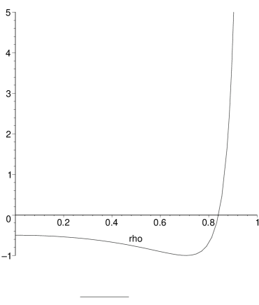
Figure 1: The moduli potential as a function of $\rho=a(t_{2})/a(t_{1})$ for ${\mathcal{I}}mT_{1,2}=0$ and $|w_{2}|>|w_{1}|>|Q|$. The radion may be stabilised with a negative vacuum energy.

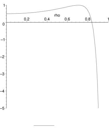
Figure 2: The moduli potential as a function of $\rho=a(t_{2})/a(t_{1})$ for ${\mathcal{I}}mT_{1,2}=0$ and $|w_{2}|<|w_{1}|<|Q|$. The radion has a metastable minimum for an infinite interbrane distance, and an unbounded from below branch leading to colliding branes.

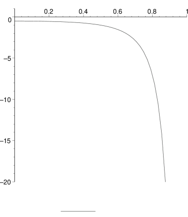
Figure 3: The moduli potential as a function of $\rho=a(t_{2})/a(t_{1})$ for ${\mathcal{I}}mT_{1,2}=0$, $|w_{2}|\leq|w_{1}|$ and $|w_{1}|>|Q|$. The radion rolls down leading to colliding branes with an infinite negative energy.

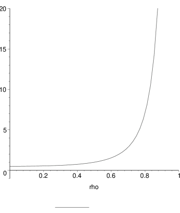
Figure 4: The moduli potential as a function of $\rho=a(t_{2})/a(t_{1})$ for ${\mathcal{I}}mT_{1,2}=0$, $|w_{2}|\geq|w_{1}|$ and $|w_{1}|<|Q|$. The radion is attracted towards a stable minimum with an infinite interbrane distance, whose positive energy can be fine-tuned to match the observed vacuum energy.

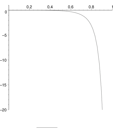
Figure 5: The moduli potential as function of $\rho=a(t_{2})/a(t_{1})$ for ${\mathcal{I}}mT_{1,2}=0$ and $|w_{2}|<|w_{1}|=|Q|$. The radion rolls down towards colliding branes with an infinite negative energy.

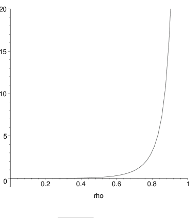
Figure 6: The moduli potential as function of $\rho=a(t_{2})/a(t_{1})$ for ${\mathcal{I}}mT_{1,2}=0$ and $|w_{2}|>|w_{1}|=|Q|$. There is a minimum with zero energy for an infinite interbrane distance.

IV.3 Soft terms

Let us now discuss the soft terms for general $w_{i}$. We restrict ourselves to the situation where matter is confined on the positive tension brane. This will allow us to evade some of the gravitational constraints due to the presence of very light moduli. We write the soft Lagrangian for the canonically normalised complex matter scalars $\tilde{s}_{i}$ as

$${\cal L}_{soft}=-m^{2}_{i\bar{j}}\tilde{s}_{i}\overline{\tilde{s}_{j}}-(\frac{1}{2}B_{ij}\tilde{s}_{i}\tilde{s}_{j}+hc)-(\frac{1}{6}A_{ijk}\tilde{s}_{i}\tilde{s}_{j}\tilde{s}_{k}+hc)$$ (68)

Note that non vanishing soft terms do not necessarily imply supersymmetry breaking (defined by non zero F–terms) when the vacuum energy cannot be neglected, as can be seen from the general expression of the soft masses (71) and B–terms (77) ; we will however keep the denomination of soft breaking terms for simplicity.

Using the usual formulae for the soft breaking terms soft , the un-normalised A–terms read

$$(A_{ijk})^{un.} = \frac{\bar{W}}{|W|}e^{K/2}F^{T_{M}}\Big{[}\partial_{T_{M}}\lambda_{ijk}(T_{p})+K_{T_{M}}\lambda_{ijk}(T_{p})-\Big{(}(\partial_{T_{M}}K_{i\bar{m}})K^{\bar{m}n}\lambda_{njk}(T_{p})$$

$$+(i\leftrightarrow j)+(i\leftrightarrow k)\Big{)}\Big{]}$$

$$\Rightarrow A_{ijk} = 12\kappa_{4}^{2}\lambda_{ijk}\alpha^{2}(k{\mathcal{I}}mT_{1})\Big{(}2\bar{w}_{2}a(\bar{T}_{2})^{3-4\alpha^{2}}a(T_{1})^{3-4\alpha^{2}}a(t_{1})^{-6}k{\mathcal{I}}mT_{2}$$ (69)

$$-\bar{w}_{1}a(\bar{T}_{1})^{6-4\alpha^{2}}a(T_{1})^{-4\alpha^{2}}a(t_{1})^{-6}(\frac{\Delta a(t_{1})^{-2}}{1+2\alpha^{2}}+2ik{\mathcal{I}}mT_{1})\Big{)}.$$

In this formula the Yukawa couplings $\lambda_{ijk}(T_{p})=a^{3}(T_{p})\lambda_{ijk}$ are the moduli-dependent ones including the cubed analytic warp factors, while $\lambda_{ijk}$ has no modulus dependence. The notation will be the same for the next terms. Notice that

$$A_{ijk}\equiv 0$$ (70)

when the imaginary parts ${\cal I}mT_{i}$ vanish. This result is akin to the vanishing of the $A$ terms in no–scale supergravity noscale , defined by the Kähler potential $K=-3ln\Big{(}\frac{\kappa_{4}^{2}}{\kappa_{5}^{2}}(T+\bar{T})-\frac{1}{3}\kappa_{4}^{2}\Sigma\bar{\Sigma}\Big{)}$. This can be understood as in the limit of vanishing bulk curvature $k\rightarrow 0$, the Kähler potential (48) takes the no-scale form.

The un-normalised soft masses for the scalars

$$(m^{2}_{i\bar{j}})^{un.}=(m_{3/2}^{2}+\kappa_{4}^{2}<V>)K_{i\bar{j}}-\overline{F^{T_{M}}}\Big{(}\partial_{\bar{T}_{M}}\partial_{T_{N}}K_{i\bar{j}}-(\partial_{T_{N}}K_{i\bar{k}})K^{\bar{k}l}(\partial_{\bar{T}_{M}}K_{l\bar{j}})\Big{)}F^{T_{N}}$$ (71)

are diagonal and read

$$m^{2}_{i\bar{j}} = \frac{2}{3}\kappa_{4}^{2}<V>\delta_{i\bar{j}}+2\alpha^{2}\kappa_{4}^{4}\delta_{i\bar{j}}\Big{|}\frac{1}{1+2\alpha^{2}}\Delta^{-1/2}a(\bar{T}_{1})^{3-4\alpha^{2}}a(t_{1})^{-2}\bar{w}_{1}$$

$$+2\Delta^{-3/2}(ki{\mathcal{I}}mT_{1})a(\bar{T}_{1})^{3-4\alpha^{2}}\bar{w}_{1}+2\Delta^{-3/2}(ki{\mathcal{I}}mT_{2})a(\bar{T}_{2})^{3-4\alpha^{2}}\bar{w}_{2}\Big{|}^{2}$$

reducing to

$$m^{2}_{i\bar{j}}=\delta_{i\bar{j}}\frac{2\kappa_{4}^{4}}{1+2\alpha^{2}}a(t_{1})^{-12\alpha^{2}}\frac{|w_{2}|^{2}\rho^{4-4\alpha^{2}}-|w_{1}|^{2}(1-\frac{\alpha^{2}}{1+2\alpha^{2}}(1-\rho^{2+4\alpha^{2}}))}{(1-\rho^{2+4\alpha^{2}})^{2}}$$ (73)

for the canonically normalised matter fields living on the first brane, and for $ImT_{i}=0$. The supergravity vacuum energy contribution $<V>$ to the soft masses is given in equation (62), or (65) for vanishing $ImT_{i}$.

The general un-normalised effective $\mu$ term on the first brane is given by

$$(\mu^{eff}_{ij})^{un.}=\frac{\bar{W}}{|W|}e^{K/2}\mu_{ij}(T_{p})+m_{3/2}\lambda_{ij}(T_{p})-\overline{F^{T_{M}}}\partial_{\bar{T}_{M}}\lambda_{ij}(T_{p})$$ (74)

where $\lambda_{ij}(T_{p})=a^{2}(t_{p})\lambda_{ij}$ are the (moduli-dependent) Giudice-Masiero couplings given in (53), not to be confused with the Yukawa couplings $\lambda_{ijk}$. The normalised effective $\mu$ term is

$$\mu^{eff}_{ij}=<\frac{\overline{W}}{|W|}>\frac{a(T_{1})^{3}}{a(t_{1})^{2}\Delta^{1/2}}\Big{(}\mu_{ij}+\lambda_{ij}\frac{\kappa_{4}^{2}w_{1}a(T_{1})^{-4\alpha^{2}}}{1+2\alpha^{2}}\Big{)}$$ (75)

reducing to

$$\mu_{ij}^{eff}=<\frac{\overline{W}}{|W|}>\frac{a(t_{1})}{\Delta^{1/2}}\Big{(}\mu_{ij}+\lambda_{ij}\frac{\kappa_{4}^{2}w_{1}a(t_{1})^{-4\alpha^{2}}}{1+2\alpha^{2}}\Big{)}$$ (76)

for vanishing imaginary parts. Note that it does not depend on the hidden brane detuning $w_{2}$, except non-relevantly through its phase pre–factor.

The general un-normalised $B$ terms are

$$(B_{ij})^{un.} = \frac{\bar{W}}{|W|}e^{K/2}\Big{[}F^{T_{M}}\Big{(}\partial_{T_{M}}\mu_{ij}(T_{p})+K_{T_{M}}\mu_{ij}(T_{p})-(\mu_{ik}(T_{p})K^{k\bar{l}}\partial_{T_{M}}K_{j\bar{l}}+i\leftrightarrow j)\Big{)}$$ (77)

$$-m_{3/2}\mu_{ij}(T_{p})\Big{]}+(2m_{3/2}^{2}+\kappa_{4}^{2}<V>)\lambda_{ij}(T_{p})-m_{3/2}\overline{F^{T_{M}}}\partial_{\bar{T}_{M}}\lambda_{ij}(T_{p})$$

$$+m_{3/2}F^{T_{M}}\Big{[}\partial_{T_{M}}\lambda_{ij}(T_{p})-(\lambda_{ik}(T_{p})K^{k\bar{l}}\partial_{T_{M}}K_{j\bar{l}}+i\leftrightarrow j)\Big{]}$$

$$-\overline{F^{T_{M}}}F^{T_{N}}\Big{[}\partial_{\bar{T}_{M}}\partial_{T_{N}}\lambda_{ij}(T_{p})-(K^{\bar{k}l}\partial_{T_{N}}K_{i\bar{k}}\partial_{\bar{T}_{M}}\lambda_{lj}(T_{p})+i\leftrightarrow j)\Big{]}$$

In our case the normalised $B$ terms become

$$B_{ij} = -\kappa_{4}^{2}(\mu^{eff}_{ij})_{\lambda=0}<\frac{W}{|W|}>\Big{[}\bar{w}_{1}\frac{a(\bar{T}_{1})^{3-4\alpha^{2}}}{(1+2\alpha^{2})a(t_{1})^{2}\Delta^{1/2}}+\bar{w}_{1}\frac{a(\bar{T}_{1})^{3-4\alpha^{2}}}{a(t_{1})^{4\alpha^{2}}\Delta^{3/2}}(4k\alpha^{2}i{\mathcal{I}}mT_{1})\Big{(}\frac{3}{2\alpha^{2}}(4k\alpha^{2}i{\mathcal{I}}mT_{1})$$ (78)

$$+\frac{3}{1+2\alpha^{2}}(a(t_{1})^{4\alpha^{2}}+a(T_{1})^{4\alpha^{2}}+\Delta a(t_{1})^{-2}\Big{)}+\bar{w}_{2}\frac{a(\bar{T}_{2})^{3-4\alpha^{2}}}{a(t_{1})^{4\alpha^{2}}\Delta^{3/2}}\frac{3}{2\alpha^{2}}(4k\alpha^{2}i{\mathcal{I}}mT_{1})(4k\alpha^{2}i{\mathcal{I}}mT_{2})\Big{]}$$

$$+2\lambda_{ij}\Delta^{-3}|w_{2}|^{2}|a(T_{2})|^{6-8\alpha^{2}}\Big{[}12\alpha^{2}k^{2}({\cal I}mT_{2})^{2}+\frac{1}{1+2\alpha^{2}}a(t_{2})^{-2+4\alpha^{2}}\Delta\Big{]}$$

$$+\lambda_{ij}[w_{1}\neq 0\rm\ terms].$$

For ${\mathcal{I}}m(T_{i})=0$ we obtain

$$B_{ij} = -\Delta^{-2}a(t_{1})\mu_{ij}\Big{[}\kappa_{4}^{2}\bar{w}_{1}a(t_{1})^{3}\frac{1-\rho^{2+4\alpha^{2}}}{1+2\alpha^{2}}\Big{]}+\lambda_{ij}\kappa_{4}^{2}<V>$$ (79)

$$+2\lambda_{ij}\kappa_{4}^{4}\Delta^{-3}{\cal R}e\Big{(}w_{1}<\overline{W}>\Big{)}a(t_{1})^{3}\frac{1-\rho^{2+4\alpha^{2}}}{1+2\alpha^{2}}$$

$$-\frac{\lambda_{ij}}{1+2\alpha^{2}}\kappa_{4}^{4}\Delta^{-2}a(t_{2})^{2+4\alpha^{2}}|w_{1}a(t_{1})^{1-4\alpha^{2}}+w_{2}a(t_{2})^{1-4\alpha^{2}}|^{2}.$$

We will give a simplified expression when discussing the phenomenology of these models. The effective Yukawa couplings are given by

$$\lambda_{ijk}^{eff}=<\frac{\overline{W}}{|W|}>\frac{a(T_{1})^{3}}{a(t_{1})^{3}}\lambda_{ijk}$$ (80)

reducing to

$$\lambda_{ijk}^{eff}=<\frac{\overline{W}}{|W|}>\lambda_{ijk}.$$ (81)

when the imaginary parts vanish.

Finally the classical gaugino masses for gauge fields living on the first brane are

$$m_{a}=-\frac{k}{2}\sum_{i=1}^{2}\beta_{a}^{i}a(t_{i})^{-4\alpha^{2}}F^{T_{i}}$$ (82)

where we have defined $\beta_{a}^{i}=\frac{\partial\ln f_{a}}{\partial\ln a(T_{i})}$ depending on the gauge coupling function $f_{a}$ for each gauge group $G_{a}$. As discussed in subsection IV.3, the case $w_{1}=0$ (positive potential) will be the one relevant phenomenologically. Considering that classically, five dimensional locality implies $\beta^{2}_{a}=0$ (as discussed in subsection III.3), we find that

$$m_{a}=0$$ (83)

as long as ${\cal I}mT_{i}=0$. There are different possibilities to generate non zero gaugino masses. For example one may add a new source of supersymmetry breaking due to a new field, like in the next section ; later in section VI we will also consider the contribution of anomaly mediated supersymmetry breaking to the gaugino masses. In the following section we will explore the possibilities opened up by the presence of a dilaton in order to generalise our construction.

V Supersymmetry Breaking and the Dilaton

V.1 The moduli potential

So far we have concentrated on the case where only one vector multiplet is present in the bulk. In this section we will focus on the case where both a vector multiplet and the universal hypermultiplet are present. The nature of the scalar potential in that case changes drastically. It becomes very intricate to study the stability of the possible extrema.

We will consider the moduli Kähler potential

$$K=-\ln(S+\bar{S})-3\ln\Big{(}a(\frac{T_{1}+\bar{T}_{1}}{2})^{2+4\alpha^{2}}-a(\frac{T_{2}+\bar{T}_{2}}{2})^{2+4\alpha^{2}}\Big{)}$$ (84)

and an arbitrary superpotential first

$$W=W(T_{1},T_{2},S)$$ (85)

where we have suppressed the dependence on the matter fields. The scalar potential reads now

$$V = \frac{|(S+\bar{S})W_{S}-W|^{2}}{(S+\bar{S})\Delta^{3}}+\frac{|W_{T_{2}}|^{2}a(t_{2})^{-2+4\alpha^{2}}-|W_{T_{1}}|^{2}a(t_{1})^{-2+4\alpha^{2}}}{3(1+2\alpha^{2})k^{2}(S+\bar{S})\Delta^{2}}$$ (86)

$$+\frac{|W_{T_{1}}a(t_{1})^{4\alpha^{2}}+W_{T_{2}}a(t_{2})^{4\alpha^{2}}+3kW|^{2}}{6\alpha^{2}k^{2}(S+\bar{S})\Delta^{3}}.$$

Notice the similarity with case when no dilaton is present. Choosing the superpotential to be of the form

$$W=w_{1}(S)a(T_{1})^{3}+w_{2}(S)a(T_{2})^{3}$$ (87)

where the two functions $w_{i}(S)$ replace the constant superpotentials $w_{i}$ of the previous section, we find that

$$V = \frac{|(S+\bar{S})W_{S}-W|^{2}}{(S+\bar{S})\Delta^{3}}$$ (88)

$$+\frac{3\kappa_{4}^{2}}{(1+2\alpha^{2})(S+\bar{S})\Delta^{2}}\Big{[}|a(T_{2})^{3-4\alpha^{2}}w_{2}(S)|^{2}a(t_{2})^{-2+4\alpha^{2}}-|a(T_{1})^{3-4\alpha^{2}}w_{1}(S)|^{2}a(t_{1})^{-2+4\alpha^{2}}\Big{]}$$

$$+\frac{24\alpha^{2}k^{2}\kappa_{4}^{2}}{(S+\bar{S})\Delta^{3}}|a(T_{1})^{3-4\alpha^{2}}w_{1}(S){\cal I}mT_{1}+a(T_{2})^{3-4\alpha^{2}}w_{2}(S){\cal I}mT_{2}|^{2}.$$

The structure of the potential when $w_{i}(S)$ are not constant is very difficult to analyse. In the following we will study the case where only one of the terms $w_{2}(S)$ is present.

V.2 Race–track models

Let us assume that strong coupling effects lead to a potential for the dilaton on the second brane. Including matter fields the superpotential reads now

$$W=a(T_{1})^{3}(\frac{1}{2}\mu\Sigma^{2}+\frac{1}{6}y\Sigma^{3})+a(T_{2})^{3}w_{2}h(S)$$ (89)

where $h(S)$ results from strong gauge coupling effects. In that case the scalar potential for the moduli reads

$$V=\kappa_{4}^{-4}e^{\hat{G}}\frac{|(S+\bar{S})h^{\prime}(S)-h(S)|^{2}}{S+\bar{S}}+\frac{|h(S)|^{2}}{S+\bar{S}}\hat{V}.$$ (90)

where hatted quantities refer to the case with no dilaton. This potential admits extrema in $S$ satisfying

$$\Big{(}(S+\bar{S})\overline{h^{\prime}(S)}-\overline{h(S)}\Big{)}h^{\prime\prime}(S)(S+\bar{S})^{2}=-\Big{(}(S+\bar{S})h^{\prime}(S)-h(S)\Big{)}\overline{h(S)}(1+\kappa_{4}^{4}e^{-\hat{G}}\hat{V}).$$ (91)

There are two types of extrema. First of all when

$$(S+\bar{S})h^{\prime}(S)=h(S)$$ (92)

we find that

$$F^{S}=0$$ (93)

Notice that $S$ is determined independently of the other moduli. In that case the potential reduces to

$$V=\frac{|h(S)|^{2}}{(S+\bar{S})}\hat{V}$$ (94)

at the extremum. The other extrema satisfy the necessary condition

$$|\frac{h^{\prime\prime}(S)}{h(S)}|(S+\bar{S})^{2}=|1+\kappa_{4}^{4}e^{-\hat{G}}\hat{V}|.$$ (95)

Let us concentrate on the gaugino condensation case (see gaugino condensate for a recent review) where

$$h(S)=\exp(-\frac{3}{2b_{0}}S)$$ (96)

The potential has then either no extremum or a maximum, i.e. the dilaton has a run–away potential, see figures 7 and 8.

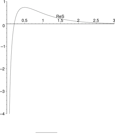
Figure 7: The moduli potential as a function of the dilaton $Re(S)$ with detunings $w_{1}=0$ and $w_{2}=exp(-\frac{3}{2b_{0}}S)$ (gaugino condensation on the hidden brane), depending on the value of $\hat{V}(T_{i})$ and $\hat{G}(T_{i})\equiv\hat{K}(T_{i})+ln|\kappa_{4}^{3}\hat{W}(T_{i})|^{2}$. Notice that $\kappa_{4}^{4}\hat{V}+e^{\hat{G}}$ is negative.

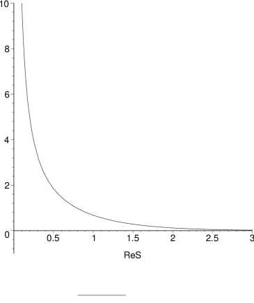
Figure 8: The moduli potential as a function of the dilaton $Re(S)$ with detunings $w_{1}=0$ and $w_{2}=exp(-\frac{3}{2b_{0}}S)$ (gaugino condensation on the hidden brane), depending on the value of $\hat{V}(T_{i})$ and $\hat{G}(T_{i})\equiv\hat{K}(T_{i})+ln|\kappa_{4}^{3}\hat{W}(T_{i})|^{2}$. Notice that $\kappa_{4}^{4}\hat{V}+e^{\hat{G}}$ is positive.

Another relevant case is the race–track superpotential on the second brane where

$$h(S)=\lambda_{1}\exp(-b_{1}S)+\lambda_{2}\exp(-b_{2}S)$$ (97)

with $b_{1},b_{2}\geq 0$. This factor originates from the gaugino condensation in two different gauge groups, and is especially motivated in our case as being known to allow for stabilization racetrack . The extrema with $F^{S}=0$ satisfy

$$\Big{|}\frac{\lambda_{2}}{\lambda_{1}}\Big{|}\exp\Big{(}(b_{1}-b_{2})Re(S)\Big{)}=\frac{1+2b_{1}Re(S)}{1+2b_{2}Re(S)}$$

$$(b_{1}-b_{2})Im(S)=\pi+arg(\frac{\lambda_{1}}{\lambda_{2}})\ (mod\ 2\pi)$$ (98)

with a unique solution in Re(S), at least when $|\frac{\lambda_{2}}{\lambda_{1}}|=1$. The stability of this configuration depends on the moduli $T_{i}$ and deserves further study.

The soft terms can be related to the soft terms when no dilaton is present. One can of course evaluate them at the various extrema.

$$y_{eff} = (S+\bar{S})^{-1/2}\hat{y}_{eff}$$

$$\mu_{eff} = (S+\bar{S})^{-1/2}\hat{\mu}_{eff}^{no\ GM}+|h(S)|(S+\bar{S})^{-1/2}\hat{\mu}_{eff}^{GM\ only}$$

$$m_{3/2} = |h(S)|(S+\bar{S})^{-1/2}\hat{m}_{3/2}$$

$$m^{2} = |h(S)|^{2}(S+\bar{S})^{-1}\hat{m}^{2}+\kappa_{4}^{-2}\frac{|F^{S}|^{2}}{(S+\bar{S})^{2}}$$

$$A = |h(S)|(S+\bar{S})^{-1}\hat{A}$$

$$B = |h(S)|(S+\bar{S})^{-1}\hat{B}^{no\ GM}+\lambda_{GM}\kappa_{4}^{-2}\frac{|F^{S}|^{2}}{(S+\bar{S})^{2}}+|h(S)|^{2}(S+\bar{S})^{-1}\hat{B}^{GM\ only}$$

$$m_{a} = |h(S)|(S+\bar{S})^{-1/2}\hat{m}_{a}$$ (99)

For most terms, this results in a simple rescaling with S-dependent factors. Note that accordingly the Giudice-Masiero parts of the effective $\mu$-term and the B-term are not rescaled like their ordinary parts. The soft masses and B-terms also have new additive contributions in $|F^{S}|^{2}$ from their vacuum energy term.

To conclude the racetrack case, we find that as long as the imaginary parts of the $T_{i}$ moduli vanish and $S$ sits at the extremum where $F^{S}=0$, the gauginos are still massless $m_{a}=0$. In section VI we will see however that the gauginos can pick up a mass via anomaly mediation.

VI Anomaly Mediated Supersymmetry Breaking

We have seen that the tree level action does not mix the moduli dependence of the gauge coupling functions coming from each brane. This is due to the locality of the coupling to the bulk scalar field in five dimensions. Now there is a quantum conformal anomaly at one loop which leads to a coupling of both moduli to the gauge sectors on each brane. We will follow closely the superfield method of anomaly in order to derive its consequences on the soft breaking terms, especially the gaugino masses and the $A$ terms.

Let us consider the supergravity action written with the chiral compensator formalism. To simplify the discussion we only consider a single matter $\Sigma$ field on the first brane

$$\int d^{4}xd^{2}\theta d^{2}\bar{\theta}\ \Big{[}-3f(t_{1},t_{2})+a^{2}(t_{1})\Big{(}|\Sigma|^{2}+\frac{1}{2}(\lambda\Sigma^{2}+\bar{\lambda}\bar{\Sigma}^{2})\Big{)}\Big{]}|\Phi|^{2}$$ (100)

$$+\int d^{4}xd^{2}\theta\ \Phi^{3}a^{3}(T_{1})[\frac{1}{2}\mu\Sigma^{2}+\frac{1}{6}y\Sigma^{3}]+h.c.$$ .

This is the action in the brane frame as can be seen from the non-canonical term $-3f(t_{1},t_{2})|\Phi|^{2}$. The coupling to the moduli has been determined in section 2. We have included a Giudice-Masiero term involving the coupling $\lambda$. The $\theta=0$ component of the conformal compensator has not yet been gauge-fixed.

In the following we will factorise real superfields $R$

$$R(\theta,\bar{\theta})=R_{0}+R_{1}\theta^{2}+\bar{R}_{1}\bar{\theta}^{2}+R_{2}\theta^{2}\bar{\theta}^{2}$$ (101)

as

$$R(\theta,\bar{\theta})=R_{0}(1+\frac{R_{1}}{R_{0}}\theta^{2})(1+\frac{\bar{R}_{1}}{\bar{R}_{0}}\bar{\theta}^{2})(1+D_{R}\theta^{2}\bar{\theta}^{2})$$ (102)

where $D_{R}=\frac{R_{2}}{R_{0}}-\frac{|R_{1}|^{2}}{R_{0}^{2}}$. We will denote by

$${\cal{R}}=R_{0}^{1/2}(1+\frac{R_{1}}{R_{0}}\theta^{2})$$ (103)

the chiral part of the factorisation of $R(\theta,\bar{\theta})$.

The change to the superspace Einstein frame is realized by the chiral superfield redefinition

$$\tilde{\Phi}={\mathcal{F}}\Phi$$ (104)

where ${\cal F}=f^{1/2}|_{\theta=0}(1+\theta^{2}\frac{1}{2}\frac{f_{t_{i}}}{f}F^{T_{i}})$. The action becomes

$$\int d^{4}xd^{2}\theta d^{2}\bar{\theta}\ \Big{[}-3(1+D_{f}\theta^{2}\bar{\theta}^{2})|\tilde{\Phi}|^{2}+\frac{|\tilde{\Phi}|^{2}}{|{\mathcal{F}}|^{2}}a^{2}(t_{1})\Big{(}|\Sigma|^{2}+\frac{1}{2}(\lambda\Sigma^{2}+\bar{\lambda}\bar{\Sigma}^{2})\Big{)}\Big{]}$$

$$+\int d^{4}xd^{2}\theta\ \frac{\tilde{\Phi}^{3}}{{\mathcal{F}}^{3}}a^{3}(T_{1})[\frac{1}{2}\mu\Sigma^{2}+\frac{1}{6}y\Sigma^{3}]+h.c.$$ (105)

The $D_{f}$ term contributes to the classical action only. One can now gauge-fix $\tilde{\Phi}|_{\theta=0}=1$ corresponding to the Einstein frame. Let us also factorise the real superfield $a^{2}(t_{1})$.

$$\int d^{4}xd^{2}\theta d^{2}\bar{\theta}\ \Big{[}-3|\tilde{\Phi}|^{2}(1+D_{f}\frac{1}{4}\theta^{2}\bar{\theta}^{2})]+\frac{|\tilde{\Phi}|^{2}|{\cal A}|^{2}}{|{\cal F}|^{2}}(1+D_{a^{2}}\theta^{2}\bar{\theta}^{2})\Big{(}|\Sigma|^{2}+\frac{1}{2}(\lambda\Sigma^{2}+\bar{\lambda}\bar{\Sigma}^{2})\Big{)}\Big{]}$$ (106)

$$+\int d^{4}xd^{2}\theta\ \frac{\tilde{\Phi}^{3}a^{3}(T_{1})}{{\mathcal{F}}^{3}}[\frac{1}{2}\mu\Sigma^{2}+\frac{1}{6}y\Sigma^{3}]+h.c.$$ .

where ${\cal A}=a(t_{1})|_{\theta=0}(1+\frac{\partial\ln a(t_{1})}{\partial t_{i}}F^{T_{i}})$. Now we can redefine the matter fields

$$\tilde{\Sigma}=\frac{\tilde{\Phi}{\cal A}}{\cal F}\Sigma\equiv{\cal G}\Sigma$$ (107)

Explicitly this reads

$$\tilde{\Sigma}=\frac{a(t_{1})}{f^{1/2}}\Big{|}_{\theta=0}(1+F_{\cal G}\theta^{2})\Sigma$$ (108)

where

$$F_{\cal G}=(F_{\tilde{\Phi}}+\frac{\partial\ln\ a(t_{1})f^{-1/2}}{\partial t_{i}}F^{T_{i}}).$$ (109)

Notice that according to this definition of $F_{\cal G}$, the $F$-term of $\cal{G}$ is actually $\frac{a(t_{1})}{f^{1/2}}\Big{|}_{\theta=0}F_{\cal G}$. The matter action becomes

$$\int d^{4}xd^{2}\theta d^{2}\bar{\theta}\Big{(}1+\theta^{2}\bar{\theta}^{2}|F^{T_{1}}|^{2}\frac{1}{a(t_{1})}\frac{\partial^{2}a(t_{1})}{(\partial t_{1})^{2}}\Big{)}\Big{(}|\tilde{\Sigma}|^{2}+\frac{1}{2}\lambda\frac{\bar{\mathcal{G}}}{\mathcal{G}}\tilde{\Sigma}^{2}+h.c.\Big{)}$$

$$+\int d^{4}xd^{2}\theta\ \frac{\tilde{\Phi}^{3}a^{3}(T_{1})}{{\mathcal{F}}^{3}{\mathcal{G}}^{3}}[\frac{1}{2}\mu{\mathcal{G}}\tilde{\Sigma}^{2}+\frac{1}{6}y\tilde{\Sigma}^{3}]+h.c.$$ (110)

This is the classical action in terms of the normalised matter fields in the Einstein frame. The superpotential action can be rewritten as

$$\int d^{4}xd^{2}\theta\ \frac{a^{3}(T_{1})}{{\mathcal{A}}^{3}}[\frac{1}{2}\mu{\mathcal{G}}\tilde{\Sigma}^{2}+\frac{1}{6}y\tilde{\Sigma}^{3}]+h.c.$$ (111)

The field redefinitions that we have performed are all anomalous. Let us now write the action with renormalized couplings, evaluated at a given energy scale $E$. The superpotential couplings are not renormalised. The effective ultra-violet field-dependent cut-off is $\Lambda_{UV}{\mathcal{G}}$ and is superfield dependent. This superfield ${\mathcal{G}}$ breaking supersymmetry when $F_{\mathcal{G}}\neq 0$, the rescaling generates anomalous soft terms. We thus have the kinetic part of the action

$$S_{qu}\supset\int d^{4}xd^{2}\theta d^{2}\bar{\theta}\Big{(}Z(\frac{E}{\Lambda_{UV}|{\mathcal{G}}|})|\tilde{\Sigma}|^{2}+\frac{1}{2}\lambda(\frac{E}{\Lambda_{UV}|{\mathcal{G}}|})\tilde{\Sigma}^{2}+h.c.\Big{)}$$ (112)

where we have discarded the $\theta^{2}\bar{\theta}^{2}|F^{T_{1}}|^{2}\frac{1}{a(t_{1})}\frac{\partial^{2}a(t_{1})}{(\partial t_{1})^{2}}$ and $\frac{\bar{\mathcal{G}}}{{\mathcal{G}}}|_{\theta\neq 0}$ terms of (110) as contributing only to the tree level soft breaking action, already computed in the previous sections, and not to the anomalous terms. Similarly, in the classical superpotential action (111), the $\frac{a^{3}(T_{1})}{{\mathcal{A}}^{3}}|_{\theta\neq 0}$ and ${\mathcal{G}}|_{\theta\neq 0}$ terms will be eliminated from now on.

Now the wave function normalization Z contains $\theta^{2}$ and $\bar{\theta}^{2}$ terms

$$Z(\frac{E}{\Lambda_{UV}|{\mathcal{G}}|})=Z(\frac{Ef^{1/2}(t_{1},t_{2})}{\Lambda_{UV}a(t_{1})})\Big{|}_{\theta=0}\Big{|}1-\frac{\gamma}{2}\theta^{2}F_{\mathcal{G}}\Big{|}^{2}\Big{(}1+\frac{1}{8}\theta^{2}\bar{\theta}^{2}(\frac{\partial\gamma}{\partial g}\beta_{g}+\frac{\partial\gamma}{\partial\ln\lambda}\xi)|F_{\mathcal{G}}|^{2}\Big{)}$$ (113)

We can redefine the matter fields using

$$\hat{\Sigma}=Z^{1/2}|_{\theta=0}\Big{(}1-\frac{\gamma}{2}\theta^{2}F_{\mathcal{G}}\Big{)}\tilde{\Sigma}.$$ (114)

where we have defined $\gamma\equiv\frac{\partial lnZ}{\partial lnE}$ the anomalous dimension of $\tilde{\Sigma}$, similarly $\xi\equiv\frac{\partial ln\lambda}{\partial lnE}$, and $\beta_{g}\equiv\frac{\partial g}{\partial lnE}$ where $g$ is a gauge coupling. The resulting action involves several blocks each leading to soft breaking terms. The soft masses come from

$$\int d^{4}xd^{2}\theta d^{2}\bar{\theta}\ (1-\theta^{2}\bar{\theta}^{2}m^{2}_{an.})|\hat{\Sigma}|^{2}$$ (115)

and read

$$m^{2}_{an.,\bar{i}j}=-\frac{1}{8}\delta_{\bar{i}j}(\frac{\partial\gamma_{i}}{\partial g}\beta_{g}+\frac{\partial\gamma_{i}}{\partial\ln\lambda_{kl}}\xi_{kl})|F_{\mathcal{G}}|^{2}$$ (116)

We have restored the index structure in the final formulae to take into account the case with several chiral multiplets, with the simplification assumption of diagonal wave function renormalisation $Z_{\bar{i}j}=Z_{i}\delta_{\bar{i}j}$. Notice that this is the generalisation of the result of Randall and Sundrum where the contribution from the moduli fields has been taken into account. The $B$ and the $\mu$ terms are also generated at one loop

$$\int d^{4}xd^{2}\theta d^{2}\bar{\theta}\frac{1}{2}\Big{(}(\lambda_{R}+\bar{\theta}^{2}\mu_{an.}-\theta^{2}\bar{\theta}^{2}B_{an.}^{G.M.})\hat{\Sigma}^{2}+h.c.\Big{)}$$

$$+\int d^{4}xd^{2}\theta\frac{1}{2}(\mu_{R}+\theta^{2}B^{\mu}_{an.})\hat{\Sigma}^{2}+h.c.$$ (117)

where $\lambda_{R,ij}=\frac{\lambda_{ij}}{\sqrt{Z_{i}Z_{j}}}$ and are given by

$$B_{an,ij}=B^{\mu}_{an,ij}+B_{an,ij}^{G.M.}$$ (118)

with

$$B_{an.,ij}^{\mu}=\frac{\gamma_{i}+\gamma_{j}}{2}F_{\mathcal{G}}\mu_{R,ij}$$ (119)

where $\mu_{R,ij}=\frac{a^{3}(T_{1})}{a^{2}(t_{1})f^{1/2}\sqrt{Z_{i}Z_{j}}}\mu_{ij}$ and

$$B_{an.,ij}^{G.M.}=\frac{1}{4}\Big{(}\frac{1}{2}\frac{\partial\xi_{ij}}{\partial g}\beta_{g}+\frac{1}{2}\frac{\partial\xi_{ij}}{\partial\ln\lambda_{kl}}\xi_{kl}-(\gamma_{i}+\gamma_{j})\xi_{ij}\Big{)}|F_{\mathcal{G}}|^{2}\lambda_{R,ij}$$ (120)

The anomalous effective $\mu$ term is given by

$$\mu_{an.,ij}=-\frac{\xi_{ij}}{2}F_{\mathcal{G}}\lambda_{R,ij}.$$ (121)

Notice that when the tree level $\mu_{eff}=0$, one can generate a loop contribution to the $\mu$ term via the Giudice–Masiero term. Finally the $A$ terms are also generated at one loop from

$$\int d^{4}xd^{2}\theta\frac{1}{6}(y_{R}+\theta^{2}A_{an.})\hat{\Sigma}^{3}+h.c.$$ (122)

where $y_{R,ijk}=\frac{a^{3}(T_{1})}{a^{3}(t_{1})\sqrt{Z_{i}Z_{j}Z_{k}}}|_{\theta=0}y_{ijk}$ leading to

$$A_{an.,ijk}=\frac{\gamma_{i}+\gamma_{j}+\gamma_{k}}{2}F_{\mathcal{G}}y_{R,ijk}$$ (123)

The order parameter for anomaly mediation is $F_{\mathcal{G}}$. The contribution in $F^{T_{i}}$ arising in $F_{\mathcal{G}}$ springs from the conformal anomaly in going from the brane frame to the Einstein frame. We have already computed $F^{T_{i}}$, we find now

$$F_{\tilde{\Phi}}=\frac{2\kappa_{4}^{2}}{3\Delta^{3/2}}\Big{(}ik{\cal I}mT_{1}a(\bar{T}_{1})^{3-4\alpha^{2}}\bar{w}_{1}+ik{\cal I}mT_{2}a(\bar{T}_{2})^{3-4\alpha^{2}}\bar{w}_{2}\Big{)}+\frac{1}{2}\frac{f_{t_{i}}}{f}F^{T_{i}}$$ (124)

This can be obtained by noticing that the superspace volume element $E^{-1}\supset\bar{\Phi}\Phi$.

Note that in principle the running couplings are now evaluated for a cut-off

$$\Lambda_{UV}\Big{|}1-\frac{\gamma}{2}\theta^{2}F_{\mathcal{G}}\Big{|}$$ (125)

which is again $\theta$-dependent. This dependence should be expanded, yielding extra contributions to the soft terms, but these would be of higher order and were consequently neglected.

Let us conclude with the anomalous gaugino masses, deduced from the running gauge coupling function

$$f(E)=f^{0}+\frac{b}{2\pi}\ln(\frac{E}{\Lambda_{UV}{\mathcal{G}}})=f_{i}^{0}+\frac{b}{2\pi}\ln(\frac{Ef^{1/2}(t_{1},t_{2})}{\Lambda_{UV}a(t_{1})}|_{\theta=0})-\frac{b}{2\pi}\theta^{2}F_{\mathcal{G}}.$$ (126)

Thus the anomalous contribution to the gaugino masses is

$$m^{an.}_{a}=\frac{b_{a}}{2\pi}F_{\mathcal{G}}.$$ (127)

Notice that all the soft terms emanating from anomaly mediation are of order $F_{\mathcal{G}}$.

VII Soft Supersymmetry Breaking from the Hidden Brane

We come back to the case where no hypermultiplet is in the bulk. Having analysed the breaking of supersymmetry in the brane models with a vector multiplet scalar field, we will extract ingredients with phenomenological relevance. We will focus on the case where the potential admits a global minimum for $\rho=0$, $w_{1}=0$, i.e. supersymmetry breaking is only due to the negative tension brane. The axions will be taken to be at the extremum ${\mathcal{I}}mT_{i}=0$, which in this case is stable for ${\mathcal{I}}mT_{2}$ and flat for ${\mathcal{I}}mT_{1}$. Notice that $F^{T_{2}}\neq 0$ implying that supersymmetry is broken.

The supersymmetry breaking can be better understood using the normalised moduli fields. We redefine the non-axionic fields in the following way:

$$a(t_{1})^{1+2\alpha^{2}} = e^{\sigma}\cosh r$$

$$a(t_{2})^{1+2\alpha^{2}} = e^{\sigma}\sinh r$$ (128)

Notice that $r=0$ when the second brane hits the singularity while $r=\infty$ when the two branes collide. The sliding field $\sigma$ describes the position of the centre of mass of the two branes. In the Einstein frame the kinetic terms are expressed as

$$S=\frac{1}{2\kappa_{4}^{2}}\int d^{4}x\sqrt{-g}({\cal R}^{(4)}-\frac{12\alpha^{2}}{1+2\alpha^{2}}(\partial\sigma)^{2}-\frac{6}{1+2\alpha^{2}}(\partial r)^{2})$$ (129)

This is a sigma–model Lagrangian with normalisation matrix $\gamma_{rr}=\frac{6}{1+2\alpha^{2}}$ and $\gamma_{\sigma\sigma}=\frac{12\alpha^{2}}{1+2\alpha^{2}}$. Notice that $\sigma$ decouples in the RS model as the centre of mass of the brane system is irrelevant. Moreover in the RS model,

$$\tanh r=e^{-kt}$$ (130)

where $t$ is the radion.

Before analysing the structure of the soft terms, let us concentrate on the $\mu$ problem. Indeed the $\mu$ term must be of the order of the weak scale. There are two sources for the $\mu$ term here, the supersymmetric $\mu$ term in the superpotential and the Giudice-Masiero term in the Kähler potential. It turns out that one cannot use the Giudice-Masiero mechanism to obtain a small $\mu$ term indeed

$$\mu^{eff}\approx\mu e^{-\frac{2\alpha^{2}}{1+2\alpha^{2}}\sigma}$$ (131)

is independent of $\lambda_{GM}$. However it is possible to use the field $\sigma$ to generate the electroweak hierarchy between a Planck scale fundamental $\mu$-term and the weak scale effective $\mu$-term. This new mechanism using the sliding field $\sigma$ is not possible in the pure Randall-Sundrum model with $\alpha=0$.

Another interesting scenario can be obtained when the classical fundamental $\mu$ term vanishes. At one loop the $\mu$ term depends on $F_{\mathcal{G}}$

$$F_{\mathcal{G}}\approx 2\kappa_{4}^{2}\bar{w}_{2}e^{-\frac{6\alpha^{2}\sigma}{1+2\alpha^{2}}}r^{\frac{3}{1+2\alpha^{2}}}$$ (132)

We thus obtain that

$$\mu=-\frac{\xi}{2}\lambda_{GM}F_{\mathcal{G}}$$ (133)

with $\xi\equiv\frac{\partial ln\lambda_{GM}}{\partial lnE}$. The $\mu$ term can be of the order of the electro–weak scale provided the $F_{\mathcal{G}}$ breaking term is in TeV range.

The soft masses are given by

$$m^{2}\approx\frac{1}{\lambda_{GM}}B$$ (134)

where the tree level contribution dominates. Hence the $B$ terms are naturally of order of the soft masses. Now the soft masses are related to $F_{\mathcal{G}}$ breaking term via

$$m^{2}\approx\frac{1}{2(1+2\alpha^{2})}\frac{|F_{\mathcal{G}}|^{2}}{r^{2}}.$$ (135)

Notice that for small $r$ the soft masses can be larger than the TeV range. Of course this can be modified provided $\xi\lambda$ is large enough. In that case $\mu\approx\xi\lambda F_{\mathcal{G}}\approx F_{\mathcal{G}}/r\approx m$ may both be at the electro–weak scale even for small $r$, at the cost of a unnatural relation between the parameters $r_{now}$ and $\xi\lambda$.

Supersymmetry is broken and the gravitino mass becomes

$$m_{3/2}\approx\frac{F_{\mathcal{G}}}{2}$$ (136)

implying that the gravitino mass can also be within the $TeV$ range.

Now the tree level gaugino masses vanish as ${\cal I}mT_{i}=0$. A non-vanishing contribution results from anomaly mediation. Therefore the anomalous contribution becomes

$$m^{an.}_{a}\approx\sqrt{\frac{1+2\alpha^{2}}{2}}\frac{b_{a}}{\pi}mr$$ (137)

This is suppressed by a $r$ factor with respect to the soft masses.

Finally the classical A term vanishes. The $A$ term picks a quantum contribution

$$A_{an}\approx 3\gamma y\sqrt{\frac{1+2\alpha^{2}}{2}}mr$$ (138)

which is suppressed by $\gamma r$ with respect to the soft masses.

We have thus characterized the mass spectrum of the superpartners. The soft terms are all determined by the supersymmetry breaking scale $F_{\mathcal{G}}$ and the value of the radion field $r$ where $r$ is driven to zero according to the scalar potential. The conclusions are unmodified for the Randall-Sundrum case $\alpha=0$.

Notice that the potential for the radion $r$ is now

$$V=\frac{3\kappa_{4}^{2}}{1+2\alpha^{2}}e^{-\frac{12\alpha^{2}}{1+2\alpha^{2}}\sigma}|w_{2}|^{2}\sinh^{\frac{4-4\alpha^{2}}{1+2\alpha^{2}}}(r)$$ (139)

driving the $r$ field to zero. As the field rolls down to its minimum, the vacuum energy becomes smaller and smaller. Notice that for small $r$

$$V\approx\frac{3}{4(1+2\alpha^{2})}\frac{|F_{\mathcal{G}}|^{2}}{\kappa_{4}^{2}}r^{-2}$$ (140)

Fine–tuning the cosmological constant for $|F_{\mathcal{G}}|\approx 1$ TeV would require $r_{now}\approx 10^{45}$. To remedy this problem, we now introduce an explicit supersymmetry breaking step. This will allow us to obtain a very small vacuum energy, so that the soft terms have the usual physical interpretation as masses and coupling constants in an almost flat space-time.

VIII Charged Branes

The branes that we have considered so far are neutral branes. One can also consider the case where a four–form lives in the bulk and couples to the bulk scalar field. This induces a new contribution to the potential for the moduli which turns out to be of the same form as the potential obtained with $w_{i}\neq 0$ detuned . The main difference here springs from the fact the we introduce the brane charges in an explicitly supersymmetry breaking form. It would be nice to embedd the charged case in a fully supersymmetric framework. A possibility would consist in using the Lagrange multiplier four–form of (8), but then the added kinetic terms would have to be supersymmetrised too.

Let us consider a four–form $C_{abcd}$ living in the bulk. We define its field strength $F=dC$ which is a five–form dual to a scalar field $*F$. The branes have charges $\pm Q$. The global charge is zero as the fifth dimension is compact. We choose the Lagrangian to be

$$S_{C}=-\frac{1}{2}\int\frac{1}{U^{2}}F\wedge*F-\frac{\sqrt{6(1-\alpha^{2})}}{1+2\alpha^{2}}\frac{\kappa_{5}Q}{\sqrt{k}}\int_{+}C+\frac{\sqrt{6(1-\alpha^{2})}}{1+2\alpha^{2}}\frac{\kappa_{5}Q}{\sqrt{k}}\int_{-}C$$ (141)

The prefactors are chosen for convenience. Notice that the coupling constant for the four–form is proportional to $U$. One can easily find the solutions of the equations of motion for $C$

$$*F=\frac{\sqrt{6(1-\alpha^{2})}}{1+2\alpha^{2}}\frac{\kappa_{5}Q}{\sqrt{k}}\epsilon(z)U^{2}$$ (142)

where $\epsilon(z)$ is the odd function jumping from -1 to 1 at the first brane and 1 to -1 at the second brane. Notice that the boundary term depends on $\int F$ and vanishes altogether. The action (141) when evaluated yields a potential in the Einstein frame which turns out to be

$$V=-\frac{3\kappa_{4}^{2}}{1+2\alpha^{2}}a(t_{1})^{-12\alpha^{2}}\frac{Q^{2}\rho^{4-4\alpha^{2}}-Q^{2}}{(1-\rho^{2+4\alpha^{2}})^{2}}$$ (143)

This is nothing but the potential for the moduli when substituting $|w_{1,2}|^{2}\to-Q^{2}$. In particular the total potential taking into account both the tension detuning and the explicit supersymmetry breaking by the charge $Q$ is now

$$V=\frac{3\kappa_{4}^{2}}{1+2\alpha^{2}}a(t_{1})^{-12\alpha^{2}}\frac{(|w_{2}|^{2}-Q^{2})\rho^{4-4\alpha^{2}}-(|w_{1}|^{2}-Q^{2})}{(1-\rho^{2+4\alpha^{2}})^{2}}$$ (144)

This potential has a much richer structure. We can distinguish five cases. We will discuss the nature of the potential as a function of $\rho=a(t_{2})/a(t_{1})$ (see figures 1, 2, 3, 4, 5 and 6).

i) $\Big{(}|w_{2}|\leq|w_{1}|$ and $|Q|<|w_{1}|\Big{)}$ or $|w_{2}|<|w_{1}|=|Q|$

The potential is negative and unbounded from below. This case is not favoured phenomenologically. This corresponds to figures 3 and 5.

ii) $|Q|<|w_{1}|<|w_{2}|$

The potential admits a negative minimum leading to anti de Sitter space. This is not a viable phenomenological case. Note that this is the only case where radion stabilisation occurs. This corresponds to figure 1 on the left hand side.

iii) $|Q|>|w_{1}|>|w_{2}|$

The potential is unbounded from below as $\rho\to 1$. Nevertheless it admits a local minimum at the origin corresponding to a positive cosmological constant. The de Sitter phase of the theory with $\rho=0$ is a metastable state protected from the unstable branch of the potential by a local maximum. Eventually the Universe would tunnel through this finite energy barrier. The resulting phase would result in a big crunch singularity due to the brane collision. This case corresponds to figure 2.

iv) $\Big{(}|w_{1}|\leq|w_{2}|$ and $|w_{1}|<Q\Big{)}$ or $|w_{2}|>|w_{1}|=|Q|$

In that case the potential is bounded from below. Its minimum is at the origin $\rho=0$. The corresponding cosmological constant is positive and can be fine–tuned to match the present value of the vacuum energy. This corresponds to figures 4 and 6 on the right hand sides.

v) $|Q|=|w_{1}|=|w_{2}|$

The potential vanishes altogether, a situation reminiscent of a BPS bound.

IX Cosmological and Gravitational Consequences

We will now investigate the cosmological consequences of the previous model where supersymmetry is broken on the hidden brane. The potential reads

$$V=\frac{3\kappa_{4}^{2}}{1+2\alpha^{2}}e^{-\frac{12\alpha^{2}}{1+2\alpha^{2}}\sigma}[Q^{2}\cosh^{\frac{4-4\alpha^{2}}{1+2\alpha^{2}}}(r)-(Q^{2}-|w_{2}|^{2})\sinh^{\frac{4-4\alpha^{2}}{1+2\alpha^{2}}}(r)]$$ (145)

Note that $\rho=\frac{a(t_{2})}{a(t_{1})}=\tanh^{\frac{1}{1+2\alpha^{2}}}(r)$. The field $r$ is driven towards its minimum at $r=0$. For small $r$ the potential reduces to an exponential potential for the sliding field $\sigma$

$$V=\frac{3\kappa_{4}^{2}\tilde{Q}^{2}(r)}{1+2\alpha^{2}}e^{-\frac{12\alpha^{2}}{1+2\alpha^{2}}\sigma}$$ (146)

where we have defined $\tilde{Q}^{2}(r)\equiv Q^{2}\cosh^{\frac{4-4\alpha^{2}}{1+2\alpha^{2}}}(r)-(Q^{2}-|w_{2}|^{2})\sinh^{\frac{4-4\alpha^{2}}{1+2\alpha^{2}}}(r)>0$, which reduces to the constant $Q^{2}$ for small enough $r$. This is a typical example of a quintessence potential for $\sigma$. The phenomenology of this type of potential is well–known. Let us summarize some of its salient features.

The exponential potential admits an attractor with scale factor

$$a=a_{0}t^{\frac{1+2\alpha^{2}}{3\alpha^{2}}}$$ (147)

which is accelerating as soon as $\alpha<1$. Even in the presence of cosmological matter such as cold dark matter, the above attractor still exists and attracts the energy fraction carried by the sliding field towards

$$\Omega_{\sigma}=1$$ (148)

i.e. the Universe becomes scalar field dominated eventually. On the attractor the equation of state of the Universe is constant

$$w=-1+\frac{4\alpha^{2}}{1+2\alpha^{2}}$$ (149)

We will see that $\alpha$ is constrained by solar system experiments leading to a tight bound on the equation of state.

These results are equivalent to solving the full 5d equations of motion with a positive detuning of the tension on the positive tension brane. In 5d the motion of the positive tension brane is at constant speed in conformal coordinates with speed $v$

$$\sqrt{1-v^{2}}=\frac{1}{1+\kappa_{5}^{2}\tilde{Q}^{2}}$$ (150)

For small $\tilde{Q}$, the brane is non–relativistic and $v=\pm\sqrt{2}\kappa_{5}\tilde{Q}$.

Of course, the Universe cannot be on the attractor now as one expects $\Omega_{\sigma}\approx.7$. Hence one must fine–tune the value of the sliding field now in such a way that

$$\tilde{Q}e^{-\frac{6\alpha^{2}}{1+2\alpha^{2}}\sigma_{now}}\approx\sqrt{\frac{1+2\alpha^{2}}{3\kappa_{4}^{2}}}\sqrt{\Omega_{\Lambda}\rho_{c}}$$ (151)

where $\Omega_{\Lambda}\approx 0.7$ and $\rho_{c}\approx 10^{-48}$ GeV⁴. Numerically this leads to

$$\tilde{Q}e^{-\frac{6\alpha^{2}}{1+2\alpha^{2}}\sigma_{now}}\approx 10^{-6}\hbox{GeV}^{3}$$ (152)

This is nothing but the usual fine–tuning of the cosmological constant. In particular, due to the smallness of the vacuum energy we can interpret the soft terms in the conventional way where the cosmological constant is set to zero. Notice that this is achieved thanks to the charge Q.

The fields $\sigma$ and $r$ are extremely light fields of masses of the order of the Hubble rate $H_{0}\approx 10^{-42}$ GeV. These extremely light fields may lead to large deviations from gravity in solar system experiments. The solar system experiments are mainly sensitive to the variation of the nucleon masses as a function of the moduli. The bulk of the nucleon masses is given by the QCD condensate $\Lambda_{QCD}$ expressed in the Einstein frame. This condensate can be estimated from the pole of the strong coupling constant at one loop and reads

$$\Lambda_{QCD}=A(\sigma,r)e^{-\frac{2\pi}{b_{3}}{\mathcal{R}}e\ f_{3}(\sigma,r,{\cal I}mT_{1})}\Lambda_{0}$$ (153)

where $f_{3}$ is the strong coupling function in the Lagrangian and $b_{3}$ is the QCD renormalisation group coefficient (the 3 index signaling the SU(3) gauge group). The overall factor $A(\sigma,r)$ accounts for the change of frame between the brane frame and the Einstein frame. The scale $e^{-\frac{2\pi}{b_{3}}{\mathcal{R}}e\ f_{3}(\Lambda_{0})}\Lambda_{0}$ is the renormalisation group invariant QCD scale in the brane frame where ordinary matter is minimally coupled to the brane metric. Explicitly we find that

$$A(\sigma,r)=e^{-\frac{2\alpha^{2}}{1+2\alpha^{2}}\sigma}\cosh^{\frac{1}{1+2\alpha^{2}}}(r)$$ (154)

The solar system experiments give tight bounds on the Eddington parameter $|\gamma_{ED}-1|\leq 10^{-5}$ testsGR . The Eddington parameter is related to $\gamma_{ED}-1\approx-2\theta$ where $\theta$ depends the coupling constants

$$\alpha_{r}=\frac{\partial\ln\Lambda_{QCD}}{\partial r},\alpha_{\sigma}=\frac{\partial\ln\Lambda_{QCD}}{\partial\sigma},\alpha_{{\cal I}mT_{1}}=\frac{\partial\ln\Lambda_{QCD}}{\partial{\cal I}mT_{1}}$$ (155)

and the normalisation of the fields $\gamma_{ij}$, with inverse matrix $\gamma^{ij}$. It is defined by

$$\theta=\gamma^{ij}\alpha_{i}\alpha_{j}=\gamma^{rr}\alpha_{r}^{2}+\gamma^{\sigma\sigma}\alpha_{\sigma}^{2}+\frac{1}{2}K^{T_{1}\bar{T}_{1}}\alpha_{{\cal I}mT_{1}}^{2}.$$ (156)

This constraint is valid for massless scalar fields, in the sense as their inverse mass is larger than solar system scales. This is the case for the moduli we consider whose inverse mass is typically of the size of the Hubble radius. Explicitly this leads to

$$\theta = \frac{1}{3}\frac{\alpha^{2}}{1+2\alpha^{2}}\Big{(}1+\frac{\pi}{b_{3}}{\mathcal{R}}ef_{3}\frac{\beta_{3}}{\alpha^{2}}(\frac{a(t_{1})}{a(T_{1})})^{4\alpha^{2}}\Big{)}^{2}+\frac{\tanh^{2}r}{6(1+2\alpha^{2})}\Big{(}1-\frac{2\pi}{b_{3}}{\mathcal{R}}ef_{3}\ \beta_{3}(\frac{a(t_{1})}{a(T_{1})})^{4\alpha^{2}}\Big{)}^{2}$$ (157)

$$+\frac{1}{12(1+2\alpha^{2})}\Big{(}1+2\alpha^{2}\tanh^{2}(r)\Big{)}\frac{4\pi^{2}}{b_{3}^{2}}\Big{(}{\mathcal{R}}ef_{3}\frac{\beta_{3}}{\alpha}(\frac{a(t_{1})}{a(T_{1})})^{4\alpha^{2}}\Big{)}^{2}.$$

Note that $\beta^{i}_{a}\equiv\frac{\partial\ln{\mathcal{R}}ef^{i}_{a}}{\partial\ln a(T_{i})}$ is now defined from the real gauge coupling ${\mathcal{R}}ef^{i}_{a}$ and not any longer from its complex version.

Imposing the experimental bounds leads to

$$\alpha<10^{-2},\ r_{now}\leq 10^{-2}$$ (158)

together with the fact that $\frac{{\mathcal{R}}ef_{3}}{\alpha}|\beta_{3}|=\frac{1}{\alpha}|\frac{\partial{\mathcal{R}}ef_{3}}{\partial lna(T_{1})}|$ cannot be too large compared to one. Considering the part of moduli-dependence due to the coupling of the gauge kinetic terms with the brane value of the bulk scalar field $\phi(T_{1})=-4\alpha\ \ln(a(T_{1}))$, one has $\frac{{\mathcal{R}}ef_{3}}{\alpha}|\beta_{3}|=4|\frac{\partial{\mathcal{R}}ef_{3}}{\partial\phi(T_{1})}|$ which has to be small compared to one.

The QCD gauge coupling $f_{3}$ is of order one and the factor $|\frac{a(t_{1})}{a(T_{1})}|$ is always smaller than one. The bound on $r_{now}$ can be fulfilled as the value $r=0$ is a minimum of the potential. Choosing $\alpha$ small enough, we find that the scalar–tensor theory is attracted towards general relativity. Notice that this leads to a very tight constraint on the equation of state of matter on the attractor $w_{\sigma}\leq-0.96$ hardly distinguishable from a pure cosmological constant.

Now let us come back to the supergravity case with a vector multiplet where $\alpha^{2}=1/12,1/3$. As can be seen the sliding field $\sigma$ leads to large deviations from ordinary gravity which are not compatible with experiments. The $\gamma^{\sigma\sigma}\alpha_{\sigma}^{2}$ contribution to the $\theta$ parameter is indeed the one proportional to $\alpha^{2}$ and thus too large in the vector multiplet case. Of course this is the usual stabilisation problem as already appearing for the dilaton. One possibility indeed would be to stabilise the $\sigma$ field. This would require to find a potential with an appropriate minimum. This is a notoriously difficult problem. Let us conclude with the pure Randall-Sundrum case $\alpha=0$. The quintessence field $\sigma$ disappears so that the gravitational constraints are now satisfied ; the vacuum energy is adjusted to its present value through the $\tilde{Q}$ parameter. This is the fine–tuning of the cosmological constant.

Hence in the Randall-Sundrum case with supersymmetric matter on the positive tension brane and detuning of the negative tension brane, the gravitational constraints are satisfied for far–away branes. In that case, the soft terms are determined by the anomaly mediation breaking term $F_{\cal G}$ and the value of the radion now. The radion is driven to zero implying that gravity is retrieved and the soft masses are very large compared to the gaugino masses and the $\mu$ term. For small values of $r$ this would lead to a naturalness problem for the electro–weak breaking. The detailed analysis of the phenomenology of these models is left for future work.

X Conclusion

We have analysed the supersymmetry breaking of 5d supergravity models with boundary branes in the presence of one vector multiplet and the universal hypermultiplet. As a particular case, this includes the supersymmetric Randall–Sundrum model. We have discussed the soft breaking terms and the moduli potential when supersymmetry is broken on both branes. We have focused on the case where matter is present on the positive tension brane and supersymmetry is broken on the negative tension brane. We have seen that the spectrum is determined both by the anomaly mediation $F_{\cal G}$ term and the normalised radion field $r$. In particular the radion $r$ is driven to zero where general relativity is retrieved. In that case the soft masses are much larger than the gaugino masses leading to a possible naturalness problem.

We have also discussed the case with the universal hypermultiplet and in particular brane race–track models. These models are very intricate and would deserve further study. In particular one may hope that the moduli may become stabilised at appropriate values.

We have seen that the supergravity models with a vector multiplet are disfavoured as leading to strong deviations from general relativity. One way of modifying this result would be for the moduli to become chameleon fields whereby their masses depend on the environment chameleon . In the solar system, this could be enough to evade the gravitational constraints and enlarge the class of phenomenologically relevant models. This is left for future work.

Acknowledgements

We would like to thank U. Ellwanger and Z. Lalak for useful comments and discussions.

Appendix A $AdS_{4}$ Supersymmetry and Radion stabilisation

Let us consider the Randall-Sundrum brane system with detuned tensions $\lambda_{1,2}=\pm\delta_{1,2}6k$ where

$$\delta_{1,2}=1-\kappa_{5}^{2}|w_{1,2}|^{2}$$ (159)

where we assume that the detuning is small

$$\kappa_{5}^{2}|w_{1,2}|^{2}\ll 1.$$ (160)

The solution of the 5d equations of motion including the brane boundary condition leads to a fixed value of the interbrane distance

$$kt=\frac{1}{2}\ln\Big{(}\frac{(\lambda+\lambda_{1})(\lambda-\lambda_{2})}{(\lambda+\lambda_{2})(\lambda-\lambda_{1})}\Big{)}$$ (161)

where $\lambda=6k$ is the tuned RS tension. For small detuning this gives

$$kt=\ln|\frac{w_{2}}{w_{1}}|.$$ (162)

Notice that stabilisation of the radion can only be achieved when $|w_{2}|>|w_{1}|$. In that case, the configuration is known to respect $AdS_{4}$ supersymmetry. We will compare this 5d analysis to the effective action approach.

In 4d at low energy, the Kähler potential

$$K=-3\ln(e^{-k(T_{1}+\bar{T}_{1})}-e^{-k(T_{2}+\bar{T}_{2})})$$ (163)

complemented with the superpotential

$$W=w_{1}e^{-3kT_{1}}+w_{2}e^{-3kT_{2}}$$ (164)

is equivalent to

$$K = -3\ln(1-e^{-k(T+\bar{T})})$$

$$W = w_{1}+w_{2}e^{-3kT}$$ (165)

up to a Kähler transformation, with $T=T_{2}-T_{1}$. The scalar potential admits a minimum when $|\frac{w_{2}}{w_{1}}|>1$ where

$$kt=\ln|\frac{w_{2}}{w_{1}}|$$ (166)

coinciding with the 5d result. At the minimum the $F^{T}$ term reads

$$F^{T}=-\frac{W}{|W|}\frac{\kappa_{4}^{2}}{k}\bar{w}_{1}(1-|\frac{w_{1}}{w_{2}}|^{2})^{-1/2}(1+e^{3ik{\cal I}mT-i\eta})$$ (167)

where $\eta$ is the phase of $\frac{w_{2}}{w_{1}}$. This vanishes for

$$3k{\cal I}mT=\eta+\pi(mod\ 2\pi)$$ (168)

leading to a configuration with a negative potential energy

$$V=-3\frac{m_{3/2}^{2}}{\kappa_{4}^{2}}$$ (169)

and a non zero gravitino mass. The solution of Einstein’s equations is then $AdS_{4}$ which breaks Poincaré invariance.

Appendix B Soft terms in the Randall-Sundrum case $\alpha=0$

In the Randall-Sundrum limit, only one chiral superfield out of the $T_{1,2}$ remains physical. We start from

$$K = -3ln(1-e^{-k(T+\bar{T})})$$

$$W = w_{1}+w_{2}e^{-3kT}$$ (170)

where $T=T_{2}-T_{1}$ is the radion superfield, and we will write $T=t+i{\cal I}mT$. As can be checked the results will be the same as those obtained from our general calculation by taking the limit $\alpha=0$. We write the soft Lagrangian for the canonically normalised complex matter scalars $\tilde{s}_{i}$ on the positive tension brane as

$${\cal L}_{soft}=-m^{2}_{i\bar{j}}\tilde{s}_{i}\overline{\tilde{s}_{j}}-(\frac{1}{2}B_{ij}\tilde{s}_{i}\tilde{s}_{j}+hc)-(\frac{1}{6}A_{ijk}\tilde{s}_{i}\tilde{s}_{j}\tilde{s}_{k}+hc).$$ (171)

The radion potential

$$V=-3\kappa_{4}^{2}\frac{|w_{1}|^{2}-e^{-4kt}|w_{2}|^{2}}{(1-e^{2kt})^{2}}$$ (172)

does not depend on ${\cal I}mT$. The gravitino mass is

$$m_{3/2}=\kappa_{4}^{2}\frac{|w_{1}+w_{2}e^{-3kT}|}{(1-e^{-2kt})^{3/2}}.$$ (173)

The radion F–term is

$$F^{T}=-\frac{\bar{W}}{|W|}\frac{\kappa_{4}^{2}}{k}\frac{\bar{w}_{1}+\bar{w}_{2}e^{-kt+3ik{\cal I}mT}}{(1-e^{-2kt})^{1/2}}.$$ (174)

The effective normalised superpotential is given by

$$\mu_{ij}^{eff} = \frac{\bar{W}}{|W|}\frac{1}{(1-e^{-2kt})^{1/2}}(\mu_{ij}+\kappa_{4}^{2}\lambda_{ij}w_{1})$$

$$\lambda^{eff}_{ijk} = \frac{\bar{W}}{|W|}\lambda_{ijk}.$$ (175)

The normalised soft mass is

$$m^{2}_{i\bar{j}}=\delta_{i\bar{j}}\frac{2}{3}\kappa_{4}^{2}V=-2\delta_{i\bar{j}}\kappa_{4}^{4}\frac{|w_{1}|^{2}-e^{-4kt}|w_{2}|^{2}}{(1-e^{2kt})^{2}}$$ (176)

and the normalised soft bilinear term is

$$B_{ij} = -\frac{\kappa_{4}^{2}\bar{w}_{1}}{1-e^{-2kt}}\mu_{ij}+\kappa_{4}^{4}\lambda_{ij}\frac{1}{(1-e^{-2kt})^{2}}$$ (177)

$$\Big{(}-|w_{1}|^{2}(1+e^{-2kt})+2|w_{2}|^{2}e^{-4kt}\Big{)}.$$

The normalised soft trilinear term is vanishing :

$$A_{ijk}=0.$$ (178)

References

• (1) P. Roy, Mechanisms of Supersymmetry Breaking in the MSSM, Pramana 60 (2003) 169-182 [arXiv:hep-ph/0207293] ; G.F. Giudice and R. Rattazzi, Theories with Gauge-Mediated Supersymmetry Breaking, Phys.Rept. 322 (1999) 419-499 [arXiv:hep-ph/9801271].
• (2) N. Arkani-Hamed, S. Dimopoulos and G. Dvali, The Hierarchy Problem and New Dimensions at a Millimeter, Phys.Lett. B429 (1998) 263-272 [arXiv:hep-ph/9803315].
• (3) L. Randall and R. Sundrum, A large mass hierarchy from a small extra dimension, Phys. Rev. Lett. 83 (1999) 3370 [arXiv:hep-ph/9905221].
• (4) N. Arkani-Hamed, S. Dimopoulos, N. Kaloper and R. Sundrum, A Small Cosmological Constant from a Large Extra Dimension, Phys.Lett. B480 (2000) 193-199 [hep-th/0001197] ; S. Kachru, M. Schulz and E. Silverstein, Self-tuning flat domain walls in 5d gravity and string theory, Phys.Rev. D62 (2000) 045021 [arXiv:hep-th/0001206].
• (5) R. Altendorfer, J. Bagger and D. Nemeschansky, Supersymmetric Randall-Sundrum scenario, Phys. Rev. D 63 (2001) 125025 [arXiv:hep-th/0003117].
• (6) A. Falkowski, Z. Lalak and S. Pokorski, Supersymmetrizing branes with bulk in five-dimensional supergravity, Phys. Lett. B 491 (2000) 172 [arXiv:hep-th/0004093].
• (7) E. Bergshoeff, R. Kallosh and A. Van Proeyen, Supersymmetry in singular spaces, JHEP 0010 (2000) 033 [arXiv:hep-th/0007044].
• (8) M. Zucker, Supersymmetric brane world scenarios from off-shell supergravity, Phys. Rev. D 64 (2001) 024024 [arXiv:hep-th/0009083].
• (9) A. Falkowski, Z. Lalak and S. Pokorski, Five-dimensional gauged supergravities with universal hypermultiplet and warped brane worlds, Phys. Lett. B 509 (2001) 337 [arXiv:hep-th/0009167].
• (10) Ph. Brax, A. Falkowski and Z. Lalak, Non-BPS branes of supersymmetric brane worlds, Phys. Lett. B 521 (2001) 105 [arXiv:hep-th/0107257].
• (11) J. Bagger and D. Belyaev, Supersymmetric branes with (almost) arbitrary tensions, Phys. Rev. D 67 (2003) 025004 [arXiv:hep-th/0206024].
• (12) P. Brax and Z. Lalak, Brane world supersymmetry, detuning, flipping and orbifolding, Acta Phys. Polon. B 33 (2002) 2399 [arXiv:hep-th/0207102].
• (13) Z. Lalak and R. Matyszkiewicz, On Scherk-Schwarz mechanism in gauged five-dimensional supergravity and on its relation to bigravity, Nucl. Phys. B 649 (2003) 389 [arXiv:hep-th/0210053].
• (14) Z. Lalak and R. Matyszkiewicz, Twisted supergravity and untwisted super-bigravity, Phys.Lett. B 562 (2003) 347-357 [arXiv:hep-th/0303227].
• (15) J. Bagger and D. Belyaev, Twisting Warped Supergravity, JHEP 0306 (2003) 013 [arXiv:hep-th/0306063].
• (16) Ph. Brax, A. Falkowski and Z. Lalak, Cosmological constant and kinetic supersymmetry breakdown on a moving brane, Nucl.Phys.B 667 (2003) 149-169 [arXiv:hep-th/0303167].
• (17) Ph. Brax and N. Chatillon, Detuned Branes and Supersymmetry Breaking, JHEP 0312 (2003) 026 [arXiv:hep-th/0309117].
• (18) M. A. Luty and R. Sundrum, Hierarchy Stabilization in Warped Supersymmetry, Phys. Rev. D 64 (2001) 065012 [arXiv:hep-th/0012158].
• (19) J. Bagger, D. Nemeschansky and R.-J. Zhang, Supersymmetric radion in the Randall-Sundrum scenario, JHEP 0108 (2001) 057 [arXiv:hep-th/0012163].
• (20) A. Falkowski, Z. Lalak and S. Pokorski, Four dimensional supergravities from five dimensional brane worlds, Nucl. Phys. B 613 (2001) 189-217 [arXiv:hep-th/0102145].
• (21) J. Bagger and M. Redi, Radion effective theory in the detuned Randall-Sundrum model, JHEP 0404 (2004) 031 [arXiv:hep-th/0312220].
• (22) J-P. Derendinger, C. Kounnas and F. Zwirner, Potentials and superpotentials in the effective N=1 supergravities from higher dimensions [arXiv:hep-th/0403043].
• (23) C. M. Will, The confrontation between General Relativity and Experiment, Living Rev.Rel. 4 (2001) 4 [arXiv:gr-qc/0103036].
• (24) Ph. Brax and C. van de Bruck, Brane Cosmology: a Review, Class. Quant. Grav. 20 (2003) R201 [arXiv:hep-th/0303095].
• (25) Ph. Brax, C. van de Bruck and A. C. Davis, Brane World Cosmology, [arXiv: hep-th/0404011].
• (26) Ph. Brax, C. van de Bruck, A.-C. Davis and C.S. Rhodes, Cosmological Evolution of Brane World Moduli, Phys.Rev. D67 (2003) 023512 [arXiv:hep-th/0209158].
• (27) C.S. Rhodes, C. van de Bruck, Ph. Brax and A.C. Davis, CMB Anisotropies in the Presence of Extra Dimensions, Phys.Rev. D68 (2003) 083511 [arXiv:astro-ph/0306343].
• (28) J. Casas, J. R. Espinoza and I. Navarro, Unconventional low-energy SUSY from warped geometry, Nucl. Phys. B620 (2002) 195 [arXiv:hep-ph/0109127].
• (29) M. A. Luty and N. Okaba, Almost No-Scale Supergravity, JHEP 0304 (2003) 050 [arXiv:hep-th/0209178].
• (30) J. Bagger, F. Ferruglio and F. Zwirner, Brane-induced supersymmetry breaking, JHEP 0202 (2002) 010 [arXiv:hep-th/0108010].
• (31) W. D. Linch III, M. A. Luty and J. Phillips, Five dimensional supergravity in N = 1 superspace, Phys. Rev. D68 (2003) 025008 [arXiv:hep-th/0209060].
• (32) I. L. Buchbinder, S. J. Gates, H. S. Goh, W. D. Linch III, M. A. Luty, S. P. Ng and J. Phillips, Supergravity loop contributions to brane world supersymmetry breaking [arXiv:hep-th/0305169].
• (33) E. Cremmer, Supergravities in 5 dimensions, in Superspace and Supergravity, Eds. S.W. Hawking and M. Rocek (Cambridge univ. press, 1981), 267.
• (34) M. Gunaydin, G. Sierra and P.K. Townsend, The geometry of N=2 Einstein supergravity and Jordan algebras, Nucl. Phys. B242 (1984) 244 ; Gauging the d=5 Maxwell-Einstein supergravity theories : more on Jordan algebras, Nucl. Phys. B253 (1985) 573.
• (35) A. Ceresole and G. Dall’Agata, General matter coupled N=2, D=5 gauged supergravity, Nucl. Phys. B585 (2000) 143-170 [arXiv:hep-th/0004111].
• (36) A. Lukas, B. A. Ovrut, K.S. Stelle and D. Waldram, Heterotic M-theory in Five Dimensions, Nucl. Phys. B 552 (1999) 246 [arXiv:hep-th/9806051].
• (37) Ph. Brax and A. C. Davis, Cosmological Solutions of Supergravity in Singular Spaces, Phys. Lett. B 497 (2001) 289, [arXiv:hep-th/0011045].
• (38) P. Brax, C. van de Bruck, A.C. Davis and C.S. Rhodes, Wave function of the radion with a bulk scalar field, Phys. Lett. B 531 (2002) 135-142 [arXiv:hep-th/0201191].
• (39) C. Charmousis, R. Gregory and V. A. Rubakov, Wave function of the radion in a brane world, Phys. Rev. D 62 (2000) 067505 [arXiv:hep-th/9912160].
• (40) T. Shiromizu, K. Maeda and M. Sasaki, The Einstein Equations on the 3-Brane World, Phys.Rev. D 62 (2000) 024012 [arXiv:gr-qc/9910076]; S. Kanno and J. Soda, Radion and Holographic Brane Gravity, Phys.Rev. D66 (2002) 083506 [arXiv:hep-th/0207029].
• (41) Ph. Brax and N. Chatillon, The 4d effective action of 5d gauged supergravity with boundaries [arXiv:hep-th/0407025].
• (42) S. Weinberg, The quantum theory of fields vol. 3 - Supersymmetry, Cambridge university press (2000).
• (43) L. Randall and R. Sundrum, Out of this world supersymmetry breaking, Nucl. Phys. B 557 (1999) 79-118 [arXiv:hep-th/9810155].
• (44) A. Brignole, L.E. Ibañez and C. Muñoz, Towards a Theory of Soft Terms for the Supersymmetric Standard Model, Nucl.Phys. B422 (1994) 125-171, Erratum-ibid. B436 (1995) 747-748 [arXiv:hep-ph/9308271].
• (45) E. Cremmer, S. Ferrara, C. Kounnas and D.V. Nanopoulos, Naturally vanishing cosmological constant in N=1 supergravity, Phys.Lett. B 133 (1983) 61.
• (46) G.F. Giudice and A. Masiero, A natural solution to the mu problem in supergravity theories, Phys.Lett. B206 (1988) 480-484.
• (47) J. Bagger and M. Redi, Supersymmetry breaking by Wilson lines in AdS5, Phys.Lett. B582 (2004) 117-120 [arXiv:hep-th/0310086].
• (48) H.P. Nilles, Gaugino Condensation and SUSY Breakdown [arXiv:hep-th/0402022].
• (49) M. Dine and Y. Shirman, Remarks on the Racetrack Scheme, Phys.Rev. D 63 (2001) 046005 [arXiv:hep-th/9906246] ; R. Ciesielski and Z. Lalak, Racetrack models in theories from extra dimensions, JHEP 0212 (2002) 028 [arXiv:hep-ph/0206134].
• (50) J. Khoury and A. Weltman, Awaiting Surprises for Tests of Gravity in Space [arXiv:astro-ph/0309300] ; J. Khoury and A. Weltman, Chameleon Cosmology, Phys.Rev. D69 (2004) 044026 [arXiv:astro-ph/0309411].