All Exact Solutions of a 1/4 Bogomol’nyi-Prasad-Sommerfield Equation

Abstract

We obtain all possible solutions of a $1/4$ Bogomol’nyi-Prasad-Sommerfield equation exactly, containing configurations made of walls, vortices and monopoles in the Higgs phase. We use supersymmetric $U(N_{\rm C})$ gauge theories with eight supercharges with $N_{\rm F}$ fundamental hypermultiplets in the strong coupling limit. The moduli space for the composite solitons is found to be the space of all holomorphic maps from a complex plane to the wall moduli space found recently, the deformed complex Grassmann manifold. Monopoles in the Higgs phase are also found in $U(1)$ gauge theory.

Dirichlet branes (D-branes) are Bogomol’nyi-Prasad-Sommerfield (BPS) states preserving a fraction of supersymmetry (SUSY) and have played a key role in non-perturbative analysis in string theory Po . (D-)strings ending on a D-brane have been realized in the effective field theory on the D-brane BIon . A $1/2$ BPS composite soliton of vortex (string) ending on a wall called a D-brane soliton has been constructed in a SUSY nonlinear sigma model (NLSM) with eight SUSY GPTT , which can be interpreted as SUSY $U(1)$ gauge theory SY1 in the strong gauge coupling limit. Solitons such as a wall junction, a string intersection were constructed both in NLSMs DW1 and gauge theories DW2 with eight SUSY. Recently a new $1/4$ BPS equation has been obtained admitting a monopole in Higgs phase as a kink on vortices mono-Higgs . The equation turns out to admit domain walls also and therefore one expects that this BPS equation allows interesting brane configurations made of these three kinds of solitons. In this Letter, we exactly give all possible solutions of the 1/4 BPS equations in the SUSY $U(N_{\rm C})$ gauge theory with $N_{\rm F}(>N_{\rm C})$ fundamental hypermultiplets in the strong gauge coupling limit, including composite solitons made of walls, vortices and monopoles. This we find the complete moduli space for these solutions. To the best of our knowledge this is the first example with completely determined moduli space for composite solitons. Our results hopefully open up a new research direction to classify and exhaust all the BPS equations, their solutions and their moduli space.

We consider a five-dimensional SUSY model with minimal kinetic terms for vector and hypermultiplets whose physical bosonic fields are ($W_{M},\Sigma$) and $H^{irA}$, respectively. The $A$-th hypermultiplet mass, the Fayet-Illiopoulos parameters, and a common gauge coupling constant for $U(N_{\rm C})$ are denoted as $m_{A}$, $c_{a},\,(a=1,2,3)$, and $g$. After eliminating auxiliary fields, the bosonic part of our Lagrangian with the scalar potential $V$ reads

$${\cal L} \!\!\!= \!\!\!-\frac{1}{2g^{2}}{\rm Tr}(F_{MN}(W)F^{MN}(W))+\frac{1}{g^{2}}{\rm Tr}({\cal D}^{M}\Sigma{\cal D}_{M}\Sigma)$$ (1)

$$\!\!\!+{\cal D}_{M}H_{irA}^{\dagger}{\cal D}^{M}H^{irA}-V,$$

$$V = \frac{g^{2}}{4}{\rm Tr}\left[\left((\sigma_{a})^{j}{}_{i}H^{i}H_{j}^{\dagger}-c_{a}{\bf 1}_{N_{\rm C}}\right)^{2}\right]$$ (2)

$$\qquad{}+H_{irA}^{\dagger}[(\Sigma-m_{A})^{2}]^{r}{}_{s}H^{isA}.$$

Covariant derivatives are ${\cal D}_{M}\Sigma=\partial_{M}\Sigma+i[W_{M},\Sigma]$, ${\cal D}_{M}H^{irA}=(\partial_{M}\delta_{s}^{r}+i(W_{M})^{r}{}_{s})H^{isA}$, and the gauge field strength is $F_{MN}(W)=-i[{\cal D}_{M},{\cal D}_{N}]$. We assume non-degenerate mass and $m_{A}>m_{A+1}$ for all $A$. The $SU(2)_{R}$ allows us to choose $c_{a}=(0,\ 0,\ c)$ with $c>0$.

Let us obtain the 1/4 BPS equations for combined solitons of walls, vortices and monopoles. A wall preserves half of the eight supercharges defined by $\gamma^{3}(i\sigma_{3})^{i}{}_{j}\varepsilon^{j}=\varepsilon^{i}$ INOS . We can obtain vortex preserving a different half defined by another projection $\gamma^{12}(i\sigma_{3})^{i}{}_{j}\varepsilon^{j}=-\varepsilon^{i}$. Combining them together, we preserve $1/4$ of supercharges. The resulting Killing spinor automatically satisfies the third projection $\gamma^{123}\varepsilon^{i}=\varepsilon^{i}$, which allows a monopole. We assume the solutions depend on $x^{1},x^{2},x^{3}$ (co-dimension three) and assume Poincaré invariance in $x^{0},x^{4}$. Then we obtain $W_{0}=W_{4}=0$. We have proved $H^{2}=0$ for 1/2 BPS saturated (pararell) walls in the case of non-degenerate masses INOS . A similar argument can be applied for the 1/4 BPS solutions to obtain $H^{2}=0$. Requiring the SUSY transformation of fermions to vanish along the above $1/4$ SUSY directions, a set of 1/4 BPS equations is obtained in the matrix notation as mono-Higgs

$$0 = {\cal D}_{3}H^{1}+\Sigma H^{1}-HM,$$ (3)

$$0 = {\cal D}_{1}H^{1}+i{\cal D}_{2}H^{1},$$ (4)

$$0 = {}^{*}F_{1}-{\cal D}_{1}\Sigma,\quad 0={}^{*}F_{2}-{\cal D}_{2}\Sigma,$$ (5)

$$0 = {}^{*}F_{3}-{\cal D}_{3}\Sigma+{g^{2}\over 2}\left(c{\bf 1}_{N_{\rm C}}-H^{1}H^{1}{}^{\dagger}\right),$$ (6)

where $(M)^{A}{}_{B}\equiv m_{A}\delta^{A}{}_{B}$ and ${}^{*}F_{m}\equiv\frac{1}{2}\epsilon_{mnl}F^{nl}(W)$ with $m=1,2,3$.

We obtain the BPS bound of the energy density $\cal E$ as ${\cal E}\geq t_{\rm w}+t_{\rm v}+t_{\rm m}+\partial_{m}J_{m}$ with $t_{\rm w},\,t_{\rm v}$ and $t_{\rm m}$ the energy densities for walls, vortices and monopoles, and the correction term $J_{m}$, which does not contribute for individual walls and vortices

$$t_{\rm w} = c\partial_{3}{\rm Tr}\Sigma,\quad t_{\rm v}=-c{\rm Tr}{}^{*}\!F_{3},$$

$$t_{\rm m} = \frac{2}{g^{2}}\partial_{m}{\rm Tr}(\Sigma{}^{*}\!F_{m}),$$ (7)

$$J_{1} = {\rm Re}\left(-i{\rm Tr}(H^{1}{}^{\dagger}{\cal D}_{2}H^{1})\right),\,J_{2}={\rm Re}\left(i{\rm Tr}(H^{1}{}^{\dagger}{\cal D}_{1}H^{1})\right),$$

$$J_{3} = -{\rm Tr}(H^{1}{}^{\dagger}(\Sigma-M)H^{1}).$$ (8)

Let us note that the magnetic flux from our monopole is measured in terms of the dual field strength multiplied (projected) by the Higgs field $\Sigma{}^{*}\!F_{m}$, as is usual to obtain the $U(1)$ field strength for the monopole in the Higgs phase mono-Higgs .

Let us construct solutions for the BPS eqs.(3)-(6), following the method to obtain complete solutions of non-Abelian walls INOS . It is crucial to observe that eq.(5) guarantees the integrability condition $[{\cal D}_{1}+i{\cal D}_{2},\,{\cal D}_{3}+\Sigma]=[\partial_{1}+i\partial_{2},\,\partial_{3}]=0$. Therefore we can introduce an $N_{\rm C}\times N_{\rm C}$ invertible complex matrix function $S(x^{m})\in GL(N_{\rm C},\mathbf{C})$ defined by

$$\Sigma+iW_{3} \equiv S^{-1}\partial_{3}S,\quad\left(({\cal D}_{3}+\Sigma)S^{-1}=0\right),$$ (9)

$$W_{1}+iW_{2} \equiv -2iS^{-1}\bar{\partial}S,\,\left(({\cal D}_{1}+i{\cal D}_{2})S^{-1}=0\right),\quad$$ (10)

where $z\equiv x^{1}+ix^{2}$, and $\bar{\partial}\equiv\partial/\partial z^{*}$. With (9) and (10), Eq. (5) is automatically satisfied, and Eqs. (3) and (4) are easily solved without any assumptions by

$$H^{1}=S^{-1}(z,z^{*},x^{3})H_{0}(z)e^{Mx^{3}}.$$ (11)

Here $H_{0}(z)$ is an arbitrary $N_{\rm C}\times N_{\rm F}$ matrix whose elements are arbitrary holomorphic functions of $z$, which we call “moduli matrix”. Let us define an $N_{\rm C}\times N_{\rm C}$ Hermitian matrix $\Omega\equiv SS^{\dagger}$, invariant under the $U(N_{\rm C})$ gauge transformations $S\rightarrow SU^{\dagger}$ with $U\in U(N_{\rm C})$. The remaining BPS eq. (6) can be rewritten in terms of this matrix $\Omega$ and the moduli matrix $H_{0}$ as

$$4\partial\bar{\partial}\Omega-4(\partial\Omega)\Omega^{-1}(\bar{\partial}\Omega)+\partial_{3}^{2}\Omega-(\partial_{3}\Omega)\Omega^{-1}(\partial_{3}\Omega)$$

$$=g^{2}\left(c\,\Omega-H_{0}\,e^{2My}H_{0}{}^{\dagger}\right).$$ (12)

Eqs.(9)–(12) determine a map from our moduli matrix $H_{0}(z)$ to all possible $1/4$ BPS solutions in three-dimensional configuration space. Let us stress that our moduli matrix $H_{0}(z)$ should be the full initial data for this map. The nonlinear partial differential eq.(12) should determine $\Omega$ in terms of the moduli matrix $H_{0}$, with the aid of appropriate boundary conditions. From the experience of walls, we expect that there is no more integration constants for $\Omega$ INOS . This expectation is explicitly borne out in the explicit solution at infinite gauge coupling as we show below.

The first two energy densities in (7) can be combined in terms of $\Omega$ as

$$t_{\rm wv}\equiv t_{\rm w}+t_{\rm v}={c\over 2}\,\partial_{m}\partial_{m}\log{\rm det}\Omega.$$ (13)

By using the BPS equations, we find the correction term of the energy density as

$$\partial_{m}J_{m}=-{1\over 2g^{2}}(\partial_{m}\partial_{m})^{2}\log{\rm det}\Omega,$$ (14)

which can be neglected if gauge coupling is large enough.

Though Eq. (12) is difficult to solve explicitly for finite gauge couplings $g$, it reduces to an algebraic equation

$$\Omega_{g\to\infty}=(SS^{\dagger})_{g\to\infty}=c^{-1}H_{0}e^{2My}H_{0}^{\dagger}$$ (15)

in the case of the infinite gauge coupling. In this limit our model reduces to the massive hyper-Kähler NLSM on the cotangent bundle over the complex Grassmann manifold, $T^{*}G_{N_{\rm F},N_{\rm C}}=T^{*}[SU(N_{\rm F})/SU(N_{\rm C})\times SU(N_{\rm F}-N_{\rm C})]$ ANS . By choosing a gauge, we obtain uniquely the $N_{\rm C}\times N_{\rm C}$ complex matrix $S$ from the $N_{\rm C}\times N_{\rm C}$ Hermitian matrix $\Omega$. Then, we find that with a given arbitrary moduli matrix $H_{0}(z)$, explicit solutions for all the quantities, $\Sigma,\,W_{m}$ and $H^{1}$ are obtained by Eqs. (9), (10) and (11). Therefore we can explicitly construct all solutions of the 1/4 BPS eqs. (3)-(6) exactly in the infinite gauge coupling.

Our explicit solution shows that the total moduli space, including all topological sectors, is fully covered by our moduli matrix $H_{0}(z)$. Eqs. (9), (10) and (11) show that a left-multiplication to $S(x^{m})$ and $H_{0}(z)$ by an arbitrary $V(z)$ of $GL(N_{\rm C},{\mathbf{C}})$, whose elements are holomorphic functions, give identical physical quantities $\Sigma,\,W_{m}$ and $H^{1}$. Since holomorphy of $H_{0}(z)$ must be respected, det$V(z)$ should be free of zeroes and singularities except at infinity. Therefore we find that the complete moduli space for solutions of the 1/4 BPS eqs. (3)-(6) is a set of whole holomorphic maps from the complex plane to the complex Grassmann manifold $G_{N_{\rm F},N_{\rm C}}=\{H_{0}|H_{0}\simeq VH_{0},\,V\in GL(N_{\rm C},{\mathbf{C}})\}$. This result can be understood by noting that we obtain for each $z$ non-Abelian multi-wall solutions whose moduli space is $G_{N_{\rm F},N_{\rm C}}$ INOS , while our 1/4 BPS solution may be regarded as a fully developed configuration of $z$-dependent “fluctuations” of moduli fields on walls. Vortices reduce to NLSM lumps SI in $g^{2}\rightarrow\infty$ Sh ; HT . When spatial infinities of $z$ are mapped into a single point in $G_{N_{\rm F},N_{\rm C}}$, the $z$ plane can be compactified to ${\bf C}P^{1}$. Then the moduli space is the whole holomorphic maps from $S^{2}\simeq{\bf C}P^{1}$ to $G_{N_{\rm F},N_{\rm C}}$, and the winding number is measured by $\pi_{2}(G_{N_{\rm F},N_{\rm C}})={\bf Z}$ with vortices winding the 2-cycles in $G_{N_{\rm F},N_{\rm C}}$. A crucial difference with ordinary lumps is that $G_{N_{\rm F},N_{\rm C}}$ is not the target space of a NLSM but the wall moduli space.

Our construction produces rich contents, even if we concentrate on the Abelian case ($N_{\rm C}=1$), which reduces to the massive NLSM on $T^{*}{\bf C}P^{N_{\rm F}-1}$ in the strong coupling limit. First consider the case where infinities of $z$ are mapped into a single point in $G_{N_{\rm F},N_{\rm C}}$. The quantity $\Omega$ reduces to a scalar

$$\Omega=\sum_{A=1}^{N_{\rm F}}|f^{A}(z)|^{2}e^{2m_{A}x^{3}}$$ (16)

with the moduli vector $H_{0}(z)=\sqrt{c}\left(f^{1}(z),\,\dots,f^{N_{\rm F}}(z)\right)$. We have $N_{\rm F}$ vacua, which are ordered by the flavor label $A$, and maximally $N_{\rm F}-1$ parallel walls interpolating between these vacua. For each fixed $z$, we can have maximally $N_{\rm F}-1$ walls at various points in $x^{3}$. By examining energy density, for instance, one can show the $\Omega$ describes a configuration close to the $A$-th vacuum, if only the $A$-th flavor is dominant in $\Omega$. If $A$-th and ($A+1$)-th flavors are comparable and dominant, it describes the $A$-th wall separating the vacua $A$ and $A+1$. The position of the $A$-th wall is easily guessed by comparing two adjacent flavors as $x_{A}^{3}(z)=\left(\log|f_{A+1}(z)|-\log|f_{A}(z)|\right)/(m_{A}-m_{A+1})$. The energy of the wall interpolating between the $A$-th and $B$-th vacua is given by

$$\int^{\infty}_{-\infty}dx^{3}t_{\rm w}={c\over 2}\Big{[}\partial_{3}\log\Omega\Big{]}^{\infty}_{-\infty}=c(m_{A}-m_{B}).$$ (17)

We find that walls are bent unless $f^{A}(z)$ is constant. Especially, if $f^{A}(z)$ has zeroes, walls are bent drastically and form vortices at those points. Actually, our solutions contain vortices stretched between walls at arbitrary positions.

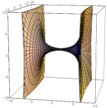
Figure 1: Surfaces defined by the same energy density $t_{\rm w}+t_{\rm v}=0.5c$: a) A vortex stretched between walls with $H_{0}(z)e^{Mx^{3}}=\sqrt{c}(e^{x^{3}},ze^{4},e^{-x^{3}})$. b) A vortex attached to a tilted wall with $H_{0}(z)e^{Mx^{3}}=\sqrt{c}(z^{2}e^{x^{3}},e^{-1/2z})$. Note that there are two surfaces with the same energy for each wall.

To see this let us choose the moduli matrix

$$f^{A}(z)=f^{A}_{0}\prod_{\alpha}(z-z^{A}_{\alpha})^{k^{A}_{\alpha}},\quad k^{A}_{\alpha}\in{\bf Z}_{+},$$ (18)

which gives vortices of vorticity $k_{\alpha}^{A}$ at $z=z^{A}_{\alpha}$ in the $A$-th vacuum. Fig.1 a) illustrates a vortex stretching between two walls, where logarithmic bending of the wall is visible towards $|z|\rightarrow\infty$. To avoid the logarithmic bending, we require $k=\sum_{\alpha}k^{A}_{\alpha}$ to be common to walls, as shown in Fig.2. We obtain the vorticity by an integration on a disc $D$ with infinite radius

$$\int_{D}d^{2}x{t_{\rm v}\over 2\pi c}=-i{1\over 2\pi}\int_{\partial D}dz\partial(\log\Omega)=k$$ (19)

using $\Omega\propto|z|^{2k}$ at $|z|\rightarrow\infty$.

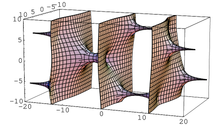
Figure 2: Multi-vorices between multi-walls: Surfaces defined by the same energy density $t_{\rm w}+t_{\rm v}=0.5c$ with $H_{0}(z)e^{Mx^{3}}=\sqrt{c}((z-4-2i)(z+5+8i)e^{3/2x^{3}},(z+8-i)(z-7+6i)e^{1/2x^{3}+12},z^{2}e^{-1/2x^{3}+12},(z-6-5i)(z+6-7i)e^{-3/2x^{3}})$.

In the effective field theory on the D-brane, a brane ending on a single brane has been obtained, but a complete solution of branes stretching between two or more branes was difficult to achieve BIon . Our construction generalizes D-brane soliton in GPTT , and may give insight into string dynamics.

A monopole in the Higgs phase was found recently in non-Abelian gauge theories mono-Higgs . We will now show that a similar monopole in the Higgs phase also exists in $U(1)$ gauge theory. Because of $1/g^{2}$ factor, the energy density of monopoles $t_{\rm m}$ vanish in the limit of infinite gauge coupling. The monopole charge $g^{2}t_{\rm m}$ is, however, finite as a kink on the vortex, precisely analogous to the non-Abelian case mono-Higgs . In a simple example of a vortex with winding number $k$ stretched between two walls, we obtain the monopole charge

$$\int_{V}d^{3}xg^{2}t_{\rm m}=-\pi|m_{A}-m_{B}|k.$$ (20)

Let us stress that our monopole in the Higgs phase should give non-vanishing contribution to the energy density once gauge coupling becomes finite.

In the case where infinities of $z$ are mapped into a single point in $G_{N_{\rm F},N_{\rm C}}$, walls are perpendicular to, and vortices are extending along, the $x^{3}$-axis in our 1/4 BPS solutions. If we relax this condition and allow an exponential function of $z$, such as $e^{mz}$, somewhere in the moduli matrix $H_{0}(z)$, the corresponding wall is no longer perpendicular to the $x^{3}$-axis. If we choose $H_{0}(z)$, for instance,

$$H_{0}e^{Mx^{3}}\!=\!\sqrt{c}(e^{m_{1}x^{3}+\tilde{m}_{1}z},\,e^{m_{2}x^{3}+\tilde{m}_{2}z}),\,\,\tilde{m}_{1,2}\in{\mathbf{C}},$$ (21)

we can guess that the wall position is expressed as $m_{1}x^{3}+{\rm Re}(\tilde{m}_{1}z)=$ $m_{2}x^{3}+{\rm Re}(\tilde{m}_{2}z)$. Actually we find the energy density $t_{\rm wv}=(c/2)\left(\Delta m^{2}+|\Delta\tilde{m}|^{2}\right){\rm sech}^{2}(X)$ to depend only on $X\equiv\Delta mx^{3}+{\rm Re}(\Delta\tilde{m}z)$ with $\Delta m=m_{1}-m_{2}$ and $\Delta\tilde{m}=\tilde{m}_{1}-\tilde{m}_{2}$. We thus find that the wall configuration is perpendicular to a vector $(\Delta m,\,{\rm Re}(\Delta\tilde{m}),\,-{\rm Im}(\Delta\tilde{m}))$. Moreover we find the dual field strength

$${}^{*}F_{3} = -2\partial\bar{\partial}\log\Omega=-{1\over 2}{|\Delta\tilde{m}|^{2}{\rm sech}^{2}(X)},$$

$${}^{*}F_{1}+i{}^{*}F_{2} = \bar{\partial}\partial_{3}\log\Omega={1\over 2}{\Delta m\Delta\tilde{m}^{*}{\rm sech}^{2}(X)},$$ (22)

flows down along the tilted wall to negative infinity of $x^{3}$: $\Delta mF_{3}+\Delta\tilde{m}\left({}^{*}F_{1}+i{}^{*}F_{2}\right)=0$. If vortices are present, they are no longer perpendicular to such tilted walls as illustrated in Fig. 1 b). This configuration offers a field theoretical model of the string ending on the D-brane with a magnetic flux HH .

We can construct a domain wall junction from two tilted walls using $H_{0}(z)$ with $\tilde{m}_{1},\,\tilde{m}_{2},\,\tilde{m}_{3}\in{\mathbf{C}}$

$$H_{0}(z)=\sqrt{c}(e^{\tilde{m}_{1}z},\,e^{\tilde{m}_{2}z},\,e^{\tilde{m}_{3}z}).$$ (23)

Positions $x^{3}_{1}(z),\,x^{3}_{2}(z)$ of the two walls can be guessed as $x^{3}_{A}(z)={\rm Re}((\tilde{m}_{A+1}-\tilde{m}_{A})z)/(m_{A}-m_{A+1})$, for $A=1,2$, which is a good estimate when $x^{3}_{1}(z)\gg x^{3}_{2}(z)$. In regions where $x^{3}_{1}(z)<x^{3}_{2}(z)$, however, we find that the configuration describes just a single wall whose position is given by the center of mass ${{\rm Re}((\tilde{m}_{3}-\tilde{m}_{1})z)}/{(m_{1}-m_{3})}$. Therefore the solution gives a junction of three walls which meet at $x^{3}=x^{3}_{1}(z)=x^{3}_{2}(z)$. These features are visible in Fig.3 where we show a “cat’s-cradle” soliton as a complicated example of composite solitons which can be easily constructed as an exact solution by our method.

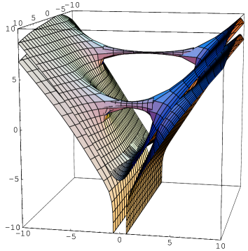
Figure 3: A cat’s-cradle soliton: Surfaces defined by the same energy density $t_{\rm w}+t_{\rm v}=0.5c$ with $H_{0}(z)e^{Mx^{3}}=\sqrt{c}(e^{x^{3}},(z-2-5i)(z-6+5i)e^{3/4z-1/2},e^{-x^{3}})$.

We have constructed composite solitons exactly in contrast to a description by the effective field theory on the host brane BIon , which is valid as an approximation for small fluctuation. Our method gives all possible solutions exactly also for non-Abelian $U(N_{\rm C})$ case easily. We have used $U(1)$ case merely to illustrate the power of our method.

References

• (1) J. Polchinski, Phys. Rev. Lett. 75, 4724 (1995).
• (2) C. G. Callan,Jr. and J. M. Maldacena, Nucl. Phys. B513, 198 (1998); G. W. Gibbons, Nucl. Phys. B514, 603 (1998); A. Hashimoto, Phys. Rev. D57, 6441 (1998).
• (3) J. P. Gauntlett, R. Portugues, D. Tong, and P.K. Townsend, Phys. Rev. D63, 085002 (2001).
• (4) M. Shifman and A. Yung, Phys. Rev. D67, 125007 (2003).
• (5) E. Abraham and P. K. Townsend, Phys. Lett. B 291, 85 (1992); J. P. Gauntlett, D. Tong, and P. K. Townsend, Phys. Rev. D63, 085001 (2001); Phys. Rev. D64, 025010 (2001); M. Naganuma, M. Nitta and N. Sakai, Grav. Cosmol. 8, 129 (2002); R. Portugues, P. K. Townsend, JHEP 0204 039, (2002); D. Tong, Phys. Rev. D66, 025013 (2002). JHEP 0304, 031 (2003); M. Arai, M. Naganuma, M. Nitta and N. Sakai, Nucl. Phys. B652, 35 (2003); M. Arai, E. Ivanov and J. Niederle, Nucl. Phys. B680, 23 (2004).
• (6) D. Tong, Phys. Rev. D66, 025013 (2002); K. Kakimoto and N. Sakai, Phys. Rev. D68, 065005 (2003). Y. Isozumi, K. Ohashi, and N. Sakai, JHEP 11, 060 (2003); JHEP 11, 061 (2003); M. Shifman and A. Yung, hep-th/0312257.
• (7) D. Tong, Phys. Rev. D69, 065003 (2004); R. Auzzi, S. Bolognesi, J. Evslin, K. Konishi and A. Yung, Nucl. Phys. B673, 187 (2003); R. Auzzi, S. Bolognesi, J. Evslin and K. Konishi, hep-th/0312233; M. Shifman and A. Yung, hep-th/0403149; A. Hanany and D. Tong, hep-th/0403158.
• (8) Y. Isozumi, M. Nitta, K. Ohashi and N. Sakai, hep-th/0404198.
• (9) M. Arai, M. Nitta, and N. Sakai, hep-th/0307274.
• (10) See, e.g., A. M. Perelomov, Phys. Rept. 146, 135 (1987).
• (11) B. J. Schroers, Nucl. Phys. B475, 440 (1996).
• (12) A. Hanany and D. Tong, JHEP 0307, 037 (2003).
• (13) K. Hashomoto, JHEP 9907, 016 (1999);A. Hashimoto and K. Hashimoto, JHEP 9911, 005 (1999).