hep-th/0405128

KEK-TH-954

May 2004

Gravitational Corrections for Supersymmetric Gauge Theories with Flavors via Matrix Models

Hiroyuki Fuji and Shun’ya Mizoguchi

Theory Division, Institute of Particle and Nuclear Studies
High Energy Accelerator Research Organization (KEK)
Tsukuba, Ibaraki 305-0801, Japan

We study the gravitational corrections to the F-term in four-dimensional ${\cal N}=1$ $U(N)$ gauge theories with flavors, using the Dijkgraaf-Vafa theory. We derive a compact formula for the annulus contribution in terms of the prime form on the matrix model curve. Remarkably, the full $\mbox{Tr}R\wedge R$ correction can be reproduced as a special momentum sector of a single $c=1$ CFT correlator, which closely resembles that in the bosonization of fermions on Riemann surfaces. The ${\cal N}=2$ limit of the torus contribution agrees with the multi-instanton calculations as well as the topological A-model result. The planar contributions, on the other hand, have no counterpart in the topological gauge theories, and we speculate about the origin of these terms.

1 Introduction

Since the discovery by Dijkgraaf and Vafa, we have recognized that non-perturbative aspects of four-dimensional supersymmetric gauge theories can be studied via matrix models. In this framework the effective superpotential for ${\cal N}=1$ supersymmetric gauge theories can be determined as the large $N$ free energy of a matrix model [1], and by minimizing it the non-perturbative vacua and their phase structures can be investigated [2]. This part of the proposal has been elegantly proven by using the chiral ring relations of ${\cal N}=1$ supersymmetry in the generalized Konishi anomaly equations [3, 4].

On the other hand, the non-planar diagrams have been shown to correspond to the gravitational corrections to the gauge theory [5, 6, 7, 8, 9, 10], in particular, the genus one free energy of the matrix model computes the gravitational F-term

$$\frac{1}{16\pi^{2}}\int d^{4}x{\cal F}_{1}(S){\rm Tr}R\wedge R.$$ (1.1)

Recently, there has been much progress in the analysis of ${\cal N}=2$ gravitational F-terms in terms of the multi-instanton calculations [11] and geometric engineering [12, 13, 14]. To compare them with the matrix model results, it is essential to know the precise form of the gravitational F-terms computed using the matrix model. For the pure gauge theory case, it has been checked that the torus free energy ${\cal F}_{1}$ coincides with the topological partition function [15] of the Donaldson-Witten theory, and hence the ${\cal N}=2$ gravitational F-terms [5, 6]. The planar free energy is also known to contribute to the gravitational corrections [16].

This framework can be extended to ${\cal N}=1$ supersymmetric gauge theories with $N_{f}$ flavors in the fundamental representation [17, 18, 19]. The dual matrix model consists of a bosonic matrix and vectors which correspond to the adjoint scalar $\phi$ and $N_{f}$ flavor fields $q^{I}$, $\tilde{q}_{I}$ ($I=1,\cdots,N_{f}$) of the gauge theory, respectively. In the vector coupled matrix model, there are two kinds loops with $\hat{N}$ and $N_{f}$ indices; the former are summed up but the latter remain as boundaries of Feynman diagrams. It looks as if the model has not only the closed string but also the open string sectors [20]. In order to evaluate $R^{2}$ terms for this gauge theory, it is necessary to consider both the torus and annulus contributions.

In this paper, we evaluate the $R^{2}$ correction terms for ${\cal N}=1$ $U(N)$ gauge theories with $N_{f}$ flavors. Using the ordinary large $N$ analysis [21], we derive a compact formula for the annulus contribution to the correction in terms of the prime form on the matrix model curve. Remarkably, the full $\mbox{Tr}R\wedge R$ correction containing the torus as well as all the planar contributions is reproduced as a special momentum sector of a single $c=1$ CFT correlator, which closely resembles that in the bosonization of fermions on Riemann surfaces. It is in accord with the recent observation in topological string theory that the non-compact B-branes correspond to fermions in a chiral boson theory on a hyper-elliptic curve [22, 23].

The plan of this paper is as follows: In section 2 we briefly review the Dijkgraaf-Vafa theory including a string theory derivation of gravitational corrections. In section 3 we compute the planar gravitational corrections for the ${\cal N}=1$ $U(N)$ gauge theories. In particular, we derive in section 3.4 a compact formula for the annulus contributions in terms of the prime form on the matrix model curve. Section 4 is devoted to some examples, in which our formula is confirmed explicitly. In section 5 we show that the full $\mbox{Tr}R\wedge R$ gravitational correction, including both the torus and planar contributions, is reproduced as a single chiral correlator of a $c=1$ conformal field theory, which closely resembles that in the bosonization of fermions on Riemann surfaces. In section 6 we consider the ${\cal N}=2$ limit, and speculate about the origin of the planar contributions. Finally, we conclude our paper with a summary and outlook on future work in section 7. The appendices contain some technical details which we need in the text.

2 Gravitational F-terms from Matrix Models

2.1 The Dijkgraaf-Vafa Theory with Flavors

The original proposal of Dijkgraaf and Vafa[1] was summarized as follows :

• The low energy effective superpotential of ${\cal N}=1$ gauge theories can be computed by summing over the planar diagrams of the matrix model with the same tree-level potential.

• The non-planar diagrams compute the gravitational F-terms for these theories.

The first statement was proven in [3], and was generalized to the cases with flavors in [18]. The latter part was also supported by many arguments [8, 9], and was explicitly confirmed in the pure gauge theory cases [5, 6].

Let us consider the ${\cal N}=1$ $U(N)$ gauge theory coupled to matter superfields $q_{I},\tilde{q}_{I}$ ($I=1,\cdots,N_{f}$) in the (anti-)fundamental representation with the superpotential [17]

$$V(\phi,q_{I}) = \mbox{tr}W(\phi)+\sum_{I=1}^{N_{f}}\tilde{q}_{I}(\phi-m_{I})q_{I},$$

$$W(\phi) = \sum_{p=1}^{n+1}\frac{g_{p}}{p}\phi^{p}.$$ (2.1)

$\phi$ is the adjoint chiral superfield. In the classical vacuum the gauge group is broken as

$$U(N) \rightarrow \prod_{i=1}^{n}U(N_{i}),~{}~{}~{}~{}~{}~{}\sum_{i=1}^{n}N_{i}=N.$$ (2.2)

The claim of [1] is that the non-perturbative vacuum structure of this theory can be analyzed by a vector coupled matrix model with action

$$S_{\mbox{\scriptsize matrix}}(\Phi,Q_{I},\tilde{Q}_{I})={\rm Tr}_{\hat{N}\times\hat{N}}W(\Phi)+\sum_{I=1}^{N_{f}}\tilde{Q}_{I}(\Phi-m_{I})Q_{I}$$ (2.3)

where $\Phi$ is an $\hat{N}\times\hat{N}$ hermitian matrix and $Q_{I}$, $\tilde{Q}_{I}$ are $\hat{N}$-component vectors. The vector-matrix coupling $\tilde{Q}_{I}\Phi Q_{I}$ leads to Feynman diagrams with boundaries in various topologies.

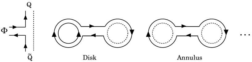
Figure 1: Feynman diagrams with boundaries.

In the low energy effective theory, the glueball superfields $S_{i}=\frac{1}{32\pi^{2}}{\rm tr}_{SU(N_{i})}W_{\alpha}W^{\alpha}$ $(i=1,\ldots,n)$ play the role of the fundamental fields. According to the proposal, $S_{i}$ is identified with the ’t Hooft coupling $g_{s}\hat{N}_{i}$ for each $i$, where $g_{s}$ is the matrix model coupling constant and $\hat{N}_{i}$ is the number of eigenvalues distributed on the $i$-th cut. Under this identification, the effective superpotential for the gauge theory is given by

$$W_{\rm eff}(S_{i})=\sum_{i=1}^{n}\left(N_{i}\frac{\partial{\cal F}_{0}^{(0)}(S_{i})}{\partial S_{i}}+\tau S_{i}\right)+{\cal F}_{0}^{(1)}(S_{i})$$ (2.4)

where ${\cal F}_{0}^{(0)}(S_{i})$ and ${\cal F}_{0}^{(1)}(S_{i})$ are given by the large $\hat{N}$ sphere and disk free energies of the matrix model, respectively. $\tau$ is the bare coupling. By extremizing this superpotential, one can analyze the non-perturbative vacuum structure of the gauge theory [2].

2.2 String Theory Derivation of Gravitational F-terms

To extend the analysis to the study of the gravitational F-terms, it is useful to consider how they arise in string theory. The gauge theory setup above can be realized in type IIB string theory on a Calabi-Yau three-fold [24, 25]

$$W^{\prime}(z)^{2}+y^{2}+v^{2}+w^{2}=0,\quad(z,y,v,w)\in\bf{C}^{4}$$ (2.5)

with $n$ singular points. By blowing them up, we obtain a smooth geometry with exceptional 2-cycles $C_{i}$ ($i=1,\cdots,n$). We then consider $N$ D5-branes wrapped around $C_{i}$’s and $N_{f}$ D5-branes around non-compact 2-cycles $C_{I}$ ($I=1,\cdots,N_{f}$). The ${\cal N}=1$ gauge theory above is realized on the space-time filling world-volume of the D5-branes.

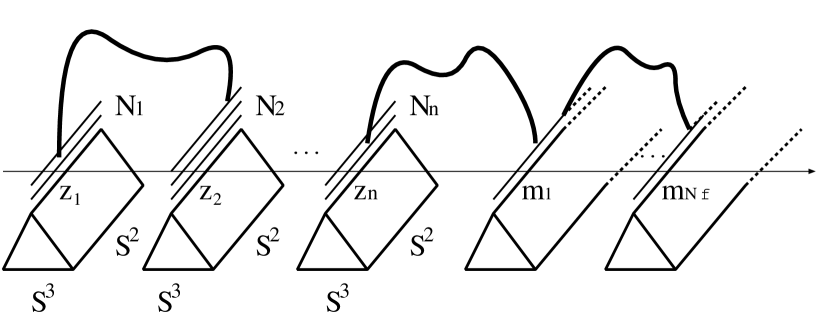
Figure 2: The brane configuration in the resolved geometry.

To evaluate the F-term corrections it is advantageous to utilize the hybrid formalism [26, 7]. The string Lagrangian density for the four-dimensional part is given by

$${\cal L}=\frac{1}{2}\partial X^{\mu}\bar{\partial}X_{\mu}+p_{\alpha}\bar{\partial}\theta^{\alpha}+p_{\dot{\alpha}}\bar{\partial}\theta^{\dot{\alpha}}+\bar{p}_{\alpha}\bar{\partial}\bar{\theta}^{\alpha}+\bar{p}_{\dot{\alpha}}\bar{\partial}\bar{\theta}^{\dot{\alpha}},$$ (2.6)

where $p$, $\bar{p}$, $\theta$ and $\bar{\theta}$ are the fermionic fields. Inserting two gluino vertex operators $\oint_{\gamma}W^{\alpha}p_{\alpha}$ on the boundaries $\gamma$ of the world-sheet, the stringy corrections lead to the F-terms containing the glueball superfields.

The string world-sheet can end either on $N$ compact or $N_{f}$ non-compact branes in the Calabi-Yau direction. Resorting to the fermion zero-mode arguments [27, 28], we can conclude that only the planar string world-sheets with at most one boundary ending on the non-compact branes can contribute to the effective superpotential [1]. A simple combinatorial argument then yields the effective superpotential (2.4) where the sphere and disk free energies of string theory are identified with those of the matrix model.

The gravitational F-term corrections are given by inserting RR vertex operators on the bulk of the string world-sheet. A candidate for such an operator is the self-dual gravitino vertex operator [7, 8]

$$\int G^{\alpha\beta\gamma}\biggl{(}p_{\alpha}X_{\beta\dot{\beta}}\bar{\partial}X_{\gamma\dot{\gamma}}+\bar{p}_{\alpha}X_{\beta\dot{\beta}}\partial X_{\gamma\dot{\gamma}}\biggr{)}\epsilon^{\dot{\beta}\dot{\gamma}}+\int G^{\alpha\beta\gamma}p_{\alpha}\bar{p}_{\beta}(\theta_{\gamma}-\bar{\theta}_{\gamma}).$$ (2.7)

Due to the chiral ring relations

$$\{W_{\alpha},W_{\beta}\}\equiv 2G_{\alpha\beta\gamma}W^{\gamma},\quad G^{4}\equiv 0\quad({\rm mod}\;\bar{D}),$$ (2.8)

at most two $G_{\alpha\beta\gamma}$ insertions can contribute to the gravitational F-term corrections. Such $G^{2}$ terms are given by the torus (Figure 3) as well as the planar world-sheet corrections (Figure 4). In particular, there are three types of planar world-sheets depending on which (compact or non-compact) branes the string ends on.

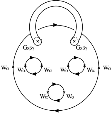
Figure 3: Gravitational corrections from the torus.

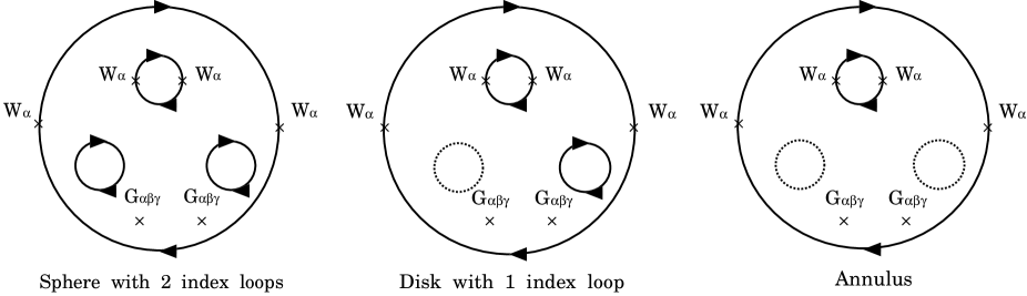
Figure 4: Three types of planar string world-sheets.

The gravitational F-term containing $G^{2}$ takes the form

$$\int d^{4}xd^{2}\theta{\cal F}_{\chi=0}(S_{i})G^{2},$$ (2.9)

where ${\cal F}_{\chi=0}(S_{i})$ ($=$ the planar $+$ torus gravitational corrections) is the contribution from the $\chi=0$ string world-sheets. If we further consider a self-dual graviphoton background $F_{\alpha\beta}$, then we also have gravitational F-terms from the graviphoton fields. Such F-terms are obtained by decomposing ${\cal N}=2$ gravitational F-terms into the ${\cal N}=1$ F-terms. It was shown in [7] that the superstring computation of these Feynman diagrams is identical to that in the field theory limit, and the combinatorial factors can be calculated in the associated matrix model.

In the following sections, we will derive a formula for the free energy ${\cal F}_{\chi=0}(S_{i})$.

3 Planar Gravitational Corrections

3.1 Gravitational Corrections from Sphere and Disk Diagrams

There are three kinds of planar diagrams which contribute to the $\mbox{Tr}R\wedge R$ correction (Figure 4). The first and second types of contributions are determined by the sphere and the disk free energies through the following combinatorial arguments: For the unbroken gauge group case (one-cut case), the coefficient of planar gravitational corrections yields

$$\sum_{h=1}^{\infty}\phantom{}{}_{h}C_{2}{\cal F}_{0,h}^{(0)}(\mbox{tr}_{SU(N)}1)^{2}S^{h-2}=\frac{N^{2}}{2}\frac{\partial^{2}{\cal F}_{0}^{(0)}(S)}{\partial S^{2}},\quad{\cal F}_{0}^{(0)}(S)=\sum_{h=1}^{\infty}{\cal F}_{0,h}^{(0)}S^{h}$$ (3.1)

for the first type, and

$$\sum_{h=1}^{\infty}\phantom{}{}_{h}C_{1}{\cal F}_{h}^{(0)}(\mbox{tr}_{SU(N)}1)^{2}S^{h-1}=N\frac{\partial{\cal F}_{0}^{(1)}(S)}{\partial S},\quad{\cal F}_{0}^{(1)}(S)=\sum_{h=1}^{\infty}{\cal F}_{0,h}^{(1)}S^{h}$$ (3.2)

for the second type. ${\cal F}_{0,h}^{(0)}$ and ${\cal F}_{0,h}^{(1)}$ are the symmetric factors of Feynman diagrams with $h$ boundaries for the sphere and disk topologies, respectively. Generalizing to the cases of arbitrary breaking patterns, we have

$$\frac{1}{2}\sum_{i,j=1}^{n}N_{i}N_{j}\frac{\partial^{2}{\cal F}^{(0)}_{0}}{\partial S_{i}\partial S_{j}}\quad(\mbox{for a sphere with 2 index loops}),$$ (3.3)

$$\sum_{i=1}^{n}N_{i}\frac{\partial{\cal F}^{(1)}_{0}}{\partial S_{i}}\quad\quad\quad\quad\;(\mbox{for a disk with 1 index loop}).$$ (3.4)

The third type of gravitational corrections come from annulus diagrams, which we will compute below using the familiar large $N$ technique in matrix models [21].

3.2 Planar Diagrams with Boundaries

Let $\Phi$ be an $\hat{N}\times\hat{N}$ hermitian matrix, and $Q^{I}$ $(I=1,\ldots,N_{f})$ be $\hat{N}$-dimensional complex vectors. We consider the partition function

$$Z = \frac{1}{\mbox{vol}~{}\!U(\hat{N})}\int d\Phi\prod_{I=1}^{N_{f}}(dQ_{I}d\tilde{Q}_{I})$$ (3.5)

$$\times\exp\left[-\frac{1}{g_{s}}\left({\rm Tr}W(\Phi)+\sum_{I=1}^{N_{f}}(\tilde{Q}_{I}\Phi Q^{I}-m_{I}\tilde{Q}_{I}Q^{I})\right)\right]$$

with a polynomial tree level potential $W(\Phi)$. It allows a topological expansion [29]

$$Z = \exp(g_{s}^{-2}{\cal F}),$$

$${\cal F} = \sum_{g=0}^{\infty}\sum_{k=0}^{\infty}g_{s}^{2g+k}{\cal F}_{g}^{(k)},$$ (3.6)

where ${\cal F}_{g}^{(k)}$ is the contributions from the connected genus $g$ diagrams with $k$ boundaries. ${\cal F}_{0}^{(0)}$ also includes the non-perturbative piece coming from the gauge volume [30].

To evaluate the annulus amplitude ${\cal F}_{0}^{(2)}$, we carry out the $dQ_{I}d\tilde{Q}_{I}$ integrations first. This yields

$$Z \propto \int d\Phi\exp\left[-\frac{1}{g_{s}}{\rm Tr}\left(W(\Phi)+g_{s}\sum_{I=1}^{N_{f}}\log(\Phi-m_{I})\right)\right]$$ (3.7)

up to an irrelevant multiplicative constant which is independent of $\Phi$, $W(\Phi)$ or $m_{I}$’s. This integrations organize a resummation of diagrams. The $g_{s}$ factor of the $\log$ potential indicates that there is a matter ($=Q\tilde{Q}$ ) loop at each $\log$ vertex. Thus, instead of $Z$, we consider the following double expansion

$$Z(g_{s},\epsilon) := \int d\Phi\exp\left[-\frac{1}{g_{s}}{\rm Tr}\left(W(\Phi)+\epsilon\sum_{I=1}^{N_{f}}\log(\Phi-m_{I})\right)\right]$$

$$:= \exp(g_{s}^{-2}{\cal F}(g_{s},\epsilon)),$$

$${\cal F}(g_{s},\epsilon) = \sum_{g=0}^{\infty}g_{s}^{2g}{\cal F}_{g}(\epsilon),$$ (3.9)

$${\cal F}_{g}(\epsilon) = \sum_{k=0}^{\infty}\epsilon^{k}{\cal F}_{g}^{(k)}$$ (3.10)

and set $\epsilon=g_{s}$. Then ${\cal F}_{1}^{(0)}$ and ${\cal F}_{0}^{(2)}$ are of same $g_{s}^{2}$ order in the ordinary $g_{s}$ expansion of the free energy; the former is the torus, whereas the latter is the annulus amplitude.

One of the aims of this paper is to determine the precise form of ${\cal F}_{0}^{(2)}$ for general $n$ and for a general polynomial potential $W(z)$, in terms of the language of Riemann surfaces that the matrix model defines. ${\cal F}_{0}^{(k)}$ $(k=1,2,\ldots)$ can be extracted from $Z(g_{s},\epsilon)$ as follows: Writing the expectation value of any function $f(\Phi)$ of $\Phi$ with respect to the measure (3.2) as $\left<f(\Phi)\right>_{g_{s},\epsilon}$, we have

$${\cal F}_{0}^{(k)} = \frac{1}{k!}\left.\frac{\partial^{k}{\cal F}_{0}(\epsilon)}{\partial\epsilon^{k}}\right|_{\epsilon=0}$$ (3.11)

$$= \frac{1}{k!}\left.\lim_{g_{s}\rightarrow 0}\frac{\partial^{k}{\cal F}(g_{s},\epsilon)}{\partial\epsilon^{k}}\right|_{\epsilon=0}$$

$$= \frac{1}{k!}\left.\lim_{g_{s}\rightarrow 0}\frac{\partial^{k-1}}{\partial\epsilon^{k-1}}\left(-g_{s}\left<\mbox{Tr}{\textstyle\sum_{I=1}^{N_{f}}}\log(\Phi-m_{I})\right>_{g_{s},\epsilon}\right)\right|_{\epsilon=0}.$$

Keeping $S:=g_{s}\hat{N}$ fixed, $g_{s}\rightarrow 0$ implies $\hat{N}\rightarrow\infty$. In this limit the expectation value can be written as

$$\lim_{g_{s}\rightarrow 0}\frac{1}{\hat{N}}\left<\mbox{Tr}f(\Phi)\right>_{g_{s},\epsilon} = \int_{-\infty}^{\infty}d\lambda\rho(\lambda,\epsilon)f(\lambda)$$ (3.12)

for any $f(\Phi)$, where $\rho(\lambda,\epsilon)$ is the eigenvalue density function of $\Phi$ normalized as

$$\int_{-\infty}^{\infty}d\lambda\rho(\lambda,\epsilon)=1.$$ (3.13)

Therefore, expanding $\rho(\lambda,\epsilon)$ as

$$\rho(\lambda,\epsilon) = \sum_{k=0}^{\infty}\epsilon^{k}\rho^{(k)}(\lambda),$$ (3.14)

we find

$${\cal F}_{0}^{(k)} = \left.\frac{1}{k!}\frac{\partial^{k-1}}{\partial\epsilon^{k-1}}\left(-S\int_{-\infty}^{\infty}d\lambda\rho(\lambda,\epsilon)\sum_{I=1}^{N_{f}}\log(\lambda-m_{I})\right)\right|_{\epsilon=0}$$ (3.15)

$$= -\frac{S}{k}\int_{-\infty}^{\infty}d\lambda\rho^{(k-1)}(\lambda)\sum_{I=1}^{N_{f}}\log(\lambda-m_{I}),$$

in particular, the disk [17, 18]

$${\cal F}_{0}^{(1)} = -S\int_{-\infty}^{\infty}d\lambda\rho^{(0)}(\lambda)\sum_{I=1}^{N_{f}}\log(\lambda-m_{I}).$$ (3.16)

and the annulus

$${\cal F}_{0}^{(2)} = -\frac{S}{2}\int_{-\infty}^{\infty}d\lambda\rho^{(1)}(\lambda)\sum_{I=1}^{N_{f}}\log(\lambda-m_{I}).$$ (3.17)

$\rho^{(k-1)}(\lambda)$ can be computed by means of the standard large $N$ technique for evaluating the planar diagrams [21].

To be rigorous, one would need to show that the $g_{s}\rightarrow 0$ limit and the operation of $\frac{\partial}{\partial\epsilon}$ commute. In Appendix A we will give a different derivation of the formula (3.17) for an arbitrary polynomial potential $W(\Phi)$ using Riemann’s bilinear identity, thereby providing an alternative proof of it.

3.3 The Large $N$ Technique

We will now briefly review the large $N$ ($=\hat{N}$) technique developed in [21] to fix our notation. (See also [31].) As we introduced above, $\rho(\lambda,g_{s})$ is the density function of the eigenvalue $\lambda$ of $\Phi$ normalized as (3.13). The nonzero support of $\rho(\lambda,g_{s})$ (as a function of $\lambda$) consists of several disjoint intervals on the real $\lambda$ axis. These intervals are the branch cuts of the resolvent $\omega(z,g_{s})$ defined by

$$\omega(z,g_{s}):=\int_{-\infty}^{\infty}d\lambda\frac{\rho(\lambda,g_{s})}{z-\lambda}$$ (3.18)

on the complex $z$ plane. (3.18) is equivalent to

$$\omega(\lambda+i0,g_{s})-\omega(\lambda-i0,g_{s}) = -2\pi i\rho(\lambda,g_{s})$$ (3.19)

in the boundary value representation. If the number of cuts is $n$, $\omega(z,g_{s})dz$ is a meromorphic differential on a hyper-elliptic curve of genus $n-1$ with a parameter $g_{s}$.

Let ${{\it\Sigma}^{g_{s}}_{n-1}}$ be a family of genus $n-1$ hyper-elliptic curves defined by the equation

$$y^{2}=\prod_{i=1}^{2n}(z-a_{i}(g_{s}))~{}~{}~{}~{}(i=1,\ldots,2n)$$ (3.20)

with a parameter $g_{s}$. We denote by $\sqrt{\prod_{i=1}^{2n}(z-a_{i}(g_{s}))}$ a branch of $y$ such that $y>0$ when $z\in\bf{R}$, $z\rightarrow\infty$. We call it the first sheet, and the other the second sheet.

The $n$ cut solution to the large $\hat{N}$ saddle point equation

$$\omega(z,g_{s})=\frac{\sqrt{\prod_{i=1}^{2n}(z-a_{i}(g_{s}))}}{4\pi iS}\sum_{j=1}^{n}\oint_{A_{j}}dw\frac{W^{\prime}(w)+\sum_{I=1}^{N_{f}}\frac{g_{s}}{w-m_{I}}}{(z-w)\sqrt{\prod_{i=1}^{2n}(w-a_{i}(g_{s}))}}$$ (3.21)

defines a meromorphic differential on ${\it\Sigma}^{g_{s}}_{n-1}$. The contour surrounds all the cuts but not the points $w=z,m_{I}$ ($I=1,\ldots,N_{f}$). The definitions of the contours are summarized in Figure 5.

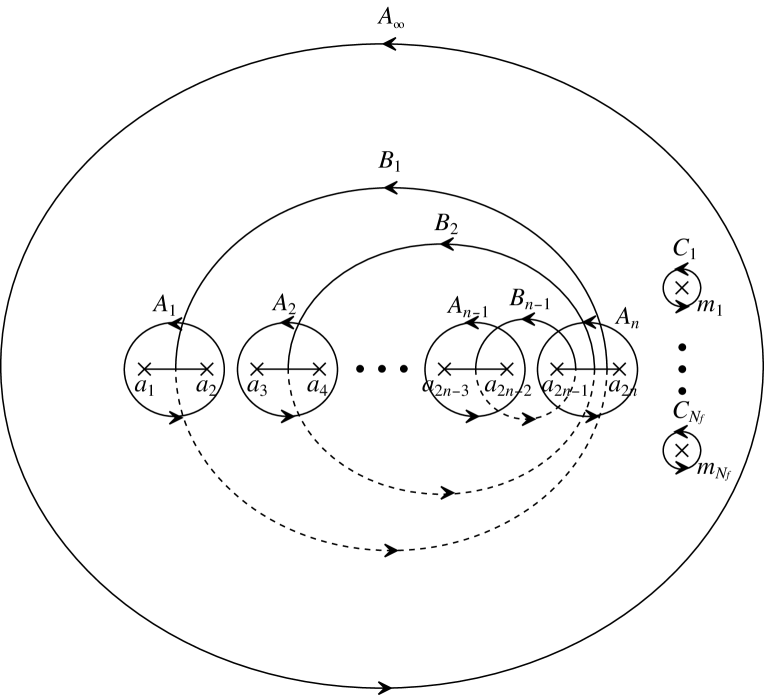
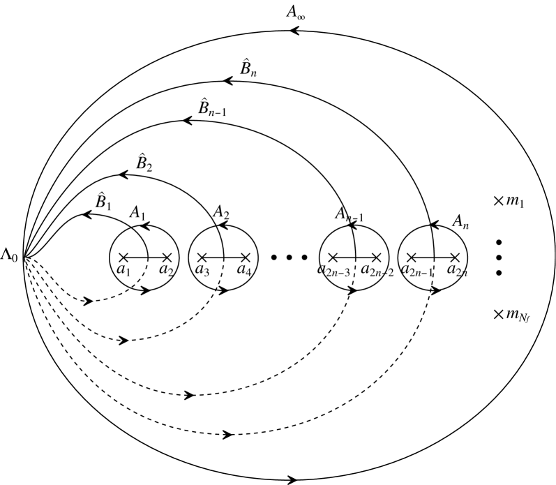
Figure 5: The contours. Those on the second sheet are shown in broken lines. $A_{\infty}$ is defined to go along $|z|=|\Lambda_{0}|$ counter-clockwise on the $z$-plane.

The positions of the $2n$ branch points $a_{i}(g_{s})$ $(i=1,\ldots,2n)$ are determined by the $2n$ conditions

$$\left(\oint_{A_{\infty}}-\sum_{I=1}^{N_{f}}\oint_{C_{I}}\right)dw\frac{\lambda^{k}(W^{\prime}(w)+\sum_{I=1}^{N_{f}}\frac{g_{s}}{w-m_{I}})}{\sqrt{\prod_{i=1}^{2n}(w-a_{i}(g_{s}))}}=4\pi iS\delta_{k,n}~{}~{}~{}(k=0,\ldots,n)$$ (3.22)

and

$$\oint_{A_{j}}dw~{}\omega(w,g_{s})=2\pi i\frac{S_{j}}{S}~{}~{}~{}(j=1,\ldots,n).$$ (3.23)

The first $n+1$ conditions (3.22) arise from the requirement that $\omega(z,g_{s})$ behaves like $\frac{1}{z}$ as $z\rightarrow\infty$ on the first sheet, whereas the latter are the conditions for a given set of filling fractions. Only $n-1$ of (3.23) are independent.

The large $\hat{N}$ free energy for the potential

$$W(\Phi,g_{s}) := W(\Phi)+g_{s}\sum_{I=1}^{N_{f}}\log(\Phi-m_{I})$$ (3.24)

is given by

$${\cal F}_{0}(g_{s}) = -S\int_{-\infty}^{\infty}d\lambda\rho(\lambda,g_{s})W(\lambda,g_{s})$$ (3.25)

$$+S^{2}\int_{-\infty}^{\infty}d\lambda\int_{-\infty}^{\infty}d\lambda^{\prime}\rho(\lambda,g_{s})\rho(\lambda^{\prime},g_{s})\log\frac{|\lambda-\lambda^{\prime}|}{\Lambda}.$$

$\Lambda$ is an arbitrary integration constant, which may be regarded as the physical scale parameter of the corresponding gauge theory up to a potential dependent constant.

3.4 Annulus Diagrams

We would now like to write (3.17) in terms of the language of Riemann surfaces. $\omega(\lambda,g_{s})$ is expanded as

$$\omega(z,g_{s}) = \sum_{k=0}^{\infty}g_{s}^{k}\omega^{(k)}(z).$$ (3.26)

The differential $\omega^{(1)}(z)dz$ must have zero A-periods because the right hand side of (3.23) does not depend on $g_{s}$.

Let us analyze the singularities of the differential $\omega^{(1)}(z)dz$. Since the discontinuity of $\omega(z,g_{s})$ is the eigenvalue density, it satisfies

$$\frac{1}{2\pi i}\sum_{j=1}^{n}\oint_{A_{j}}dz\;\omega(z,g_{s})=1.$$ (3.27)

$\omega(z,g_{s})$ also satisfies

$$\frac{1}{2\pi i}\oint_{A_{\infty}}dz\;\omega(z,g_{s})=1$$ (3.28)

because $\omega(z,g_{s})$ goes to $\frac{1}{z}$ at infinity on the first sheet. (3.27)(3.28) imply that $\omega(z,g_{s})dz$ has a pole of first order at $z=\infty$ on the first sheet with residue $-1$, but otherwise it is regular everywhere else on the first sheet. Therefore we conclude that $\omega^{(1)}(z)dz$ is regular everywhere on the first sheet. On the other hand, $\omega(z,g_{s})$ can be written in the form

$$\omega(z,g_{s}) = \frac{1}{2S}\left(W^{\prime}(z)+\sum_{I}\frac{g_{s}}{z-m_{I}}-y(z,g_{s})\right),$$

$$y(z,g_{s}) = -\frac{\sqrt{\prod_{i=1}^{2n}(z-a_{i}(g_{s}))}}{2\pi i}\left(\oint_{A_{\infty}}-\sum_{I=1}^{N_{f}}\oint_{C_{I}}\right)dw\frac{W^{\prime}(w)+\sum_{I=1}^{N_{f}}\frac{g_{s}}{\lambda-m_{I}}}{(z-w)\sqrt{\prod_{i=1}^{2n}(w-a_{i}(g_{s}))}}.$$

We similarly expand

$$y(z,g_{s})=\sum_{k=0}^{\infty}g_{s}^{k}y^{(k)}(z).$$ (3.30)

Note that the difference of the contours of $y(z,g_{s})$ and $\omega(z,g_{s})$; thanks to this change, the contour integral of $y(z,g_{s})$ gives some rational function of $z$. This implies that $y(z,g_{s})$ changes its sign under the interchange of the first and second sheets.

Since the second term of $\omega(z,g_{s})$ has a first order singularity at each $z=m_{I}$ $(I=1,\ldots,N_{f})$ with residue $\frac{g_{s}}{2S}$ and at $z=\infty$ with residue $-\frac{g_{s}N_{f}}{2S}$ on both sheets, the $y(z,g_{s})$ term must cancel them on the first sheet, and hence in turn doubles the residues on the second sheet. To summarize, denoting coordinates on the second sheet with tildes, $\omega^{(1)}(z)dz$ has first order singularities at

• $z=\tilde{m}_{I}$ with residue $\frac{1}{S}$ for all $I=1,\ldots,N_{f}$, and

• $z=\tilde{\infty}$ with residue $-\frac{N_{f}}{S}$,

otherwise holomorphic everywhere else on ${\it\Sigma}^{g_{s}}_{n-1}$. Thus we have shown that $\omega^{(1)}(z)dz$ is an abelian differential of the third kind with zero A-periods and is given by

$$\omega^{(1)}(z)dz=\frac{1}{S}\sum_{I=1}^{N_{f}}\omega_{\tilde{m}_{I}-\tilde{\infty}},$$ (3.31)

where, following the notation used in [32], $\omega_{a-b}(z)$ denotes a zero A-period abelian differential which has simple poles at $z=a,b$ with residue $\pm 1$, respectively.

One of the nice things for this kind of differentials is that their integrals are compactly described in terms of the prime form $E(z,w)$ on ${\it\Sigma}^{g_{s}}_{n-1}$. The prime form $E(z,w)$ is known to be the unique bi-holomorphic half differential on a compact Riemann surface such that $E(z,w)=0$ if and only if $z=w$. One of the basic properties of the prime form is [32]

$$\omega_{a-b}(z) = d_{z}\log\frac{E(z,a)}{E(z,b)}.$$ (3.32)

Using this formula, we finally obtain the third type of contributions to the gravitational correction

$${\cal F}_{0}^{(2)} = -\frac{1}{4\pi i}\sum_{j=1}^{n}\oint_{A_{j}}\sum_{J=1}^{N_{f}}\omega_{\tilde{m}_{J}-\tilde{\infty}}(z)\sum_{I=1}^{N_{f}}\log(z-m_{I})$$ (3.33)

$$= \frac{1}{2}\sum_{I,J=1}^{N_{f}}\int_{m_{I}}^{\infty}\omega_{\tilde{m}_{J}-\tilde{\infty}}(z)$$

$$= \frac{1}{2}\sum_{I,J=1}^{N_{f}}\log\frac{E(m_{I},\tilde{\infty})E(\infty,\tilde{m}_{J})}{E(m_{I},\tilde{m}_{J})E(\infty,\tilde{\infty})}.$$

The full planar gravitational correction ${\cal F}^{(\mbox{\scriptsize pl})}$ is thus

$${\cal F}^{(\mbox{\scriptsize pl})} = \frac{1}{2}\sum_{i,j=1}^{n}N_{i}N_{j}\frac{\partial^{2}{\cal F}^{(0)}_{0}}{\partial S_{i}\partial S_{j}}+\sum_{i=1}^{n}N_{i}\frac{\partial{\cal F}^{(1)}_{0}}{\partial S_{i}}+{\cal F}^{(2)}_{0}$$ (3.34)

with

$$\frac{1}{2}\sum_{i,j=1}^{n}N_{i}N_{j}\frac{\partial^{2}{\cal F}_{0}^{(0)}}{\partial S_{i}\partial S_{j}} = \lim_{|\Lambda_{0}|\rightarrow\infty}\left[\sum_{i,j=1}^{n}N_{i}N_{j}\left(-\pi i\int_{\hat{B}_{i}}\hat{\omega}_{j}(z)+\log\frac{-\Lambda_{0}}{\Lambda}\right)\right],$$ (3.35)

$$\sum_{i=1}^{n}N_{i}\frac{\partial{\cal F}_{0}^{(1)}}{\partial S_{i}} = -\sum_{i,k=1}^{n}N_{i}\oint_{A_{k}}\hat{\omega}_{i}(z)\sum_{I=1}^{N_{f}}\log(z-m_{I})$$ (3.36)

$$= \lim_{|\Lambda_{0}|\rightarrow\infty}\left[\rule{0.0pt}{19.91692pt}\right.\sum_{i=1}^{n}N_{i}\sum_{I=1}^{N_{f}}\left(2\pi i\int_{m_{I}}^{\Lambda_{0}}\hat{\omega}_{i}(z)-\log(-\Lambda_{0})\right)\left.\rule{0.0pt}{19.91692pt}\right]$$

and ${\cal F}_{0}^{(2)}$ given in (3.33). In deriving the above, we have used the special geometry relation [1, 18]

$$\frac{\partial{\cal F}_{0}^{(0)}}{\partial S_{i}} = \lim_{|\Lambda_{0}|\rightarrow\infty}\left(\frac{1}{2}\int_{\hat{B}_{i}}dz\;y^{(0)}(z)-W(\Lambda_{0})+2S\log\frac{-\Lambda_{0}}{\Lambda}\right)$$ (3.37)

as well as the variation formula

$$\frac{\partial y^{(0)}(z)}{\partial S_{i}}dz = -4\pi i\hat{\omega}_{i}(z)(i=1,\ldots,n),$$ (3.38)

where $\hat{\omega}_{i}$ $(i=1,\ldots,n)$ are related with the holomorphic differentials $\omega_{i}$ $(i=1,\ldots,n-1)$ on ${\it\Sigma}^{g_{s}=0}_{n-1}$ through the relations

$$\hat{\omega}_{i} = \omega_{i}-\frac{1}{2\pi i}\omega_{\infty-\tilde{\infty}}~{}~{}~{}(i=1,\ldots,n-1),$$

$$\hat{\omega}_{n} = -\frac{1}{2\pi i}\omega_{\infty-\tilde{\infty}}.$$ (3.39)

They are normalized so that

$$\oint_{A_{i}}\omega_{j}(z) = \delta_{ij}~{}~{}~{}(i,j=1,\ldots,n-1),$$

$$\oint_{A_{i}}\hat{\omega}_{j}(z) = \delta_{ij}~{}~{}~{}(i,j=1,\ldots,n).$$ (3.40)

See Appendix B for details.

4 Examples

4.1 One-cut Solutions for Quadratic Potential with $N_{f}=1$

The first example is the ‘conifold’ case

$$W(\Phi) = -t\Phi^{2}$$ (4.1)

with a single matter field. The resolvent $\omega(z,g_{s})$ is

$$\omega(z,g_{s}) = \frac{1}{2S}\left[\rule{0.0pt}{19.91692pt}-2tz+\frac{g_{s}}{z-m}\right.$$

$$\left.+\sqrt{(z-c(g_{s}))^{2}-\mu(g_{s})^{2}}\left(2t-\frac{\frac{g_{s}}{z-m}}{\sqrt{(m-c(g_{s}))^{2}-\mu(g_{s})^{2}}}\right)\right],$$

where $c(g_{s})$ and $\mu(g_{s})$ are related with the positions of the end points by

$$a_{1}(g_{s}) = c(g_{s})+\mu(g_{s}),$$

$$a_{2}(g_{s}) = c(g_{s})-\mu(g_{s})$$ (4.3)

and satisfy (3.22) and (3.23)

$$0 = 2tc(g_{s})+\frac{g_{s}}{\sqrt{(m-c(g_{s}))^{2}-\mu(g_{s})^{2}}},$$ (4.4)

$$2S = -t\mu(g_{s})^{2}+g_{s}\left(1-\frac{m-c(g_{s})}{\sqrt{(m-c(g_{s}))^{2}-\mu(g_{s})^{2}}}\right).$$ (4.5)

They are solved as a power series

$$c(g_{s}) = -\frac{1}{2t\sqrt{m^{2}-\mu^{2}}}g_{s}+\frac{-\sqrt{m^{2}-\mu^{2}}+2m}{2t^{2}(m^{2}-\mu^{2})^{2}}g_{s}^{2}+{\cal O}(g_{s}^{3}),$$ (4.6)

$$\mu(g_{s}) = \mu+\frac{\sqrt{m^{2}-\mu^{2}}-m}{2t\mu\sqrt{m^{2}-\mu^{2}}}g_{s}+\frac{-(m^{2}-2\mu^{2}-m\sqrt{m^{2}-\mu^{2}})^{2}+5\mu^{4}}{4t^{2}\mu^{3}(m^{2}-\mu^{2})^{2}}g_{s}^{2}+{\cal O}(g_{s}^{3})$$

with $\mu:=\sqrt{-\frac{2S}{t}}$. The integral for the genus zero free energy ${\cal F}_{0}$ (3.25) can be completely performed in this case and is given in Appendix C. ${\cal F}_{0}^{(1)}$ (the disk amplitude) and ${\cal F}_{0}^{(2)}$ (the annulus amplitude) are obtained as coefficients of the Taylor series of ${\cal F}_{0}(g_{s})$. After some calculations using (4.6) and (LABEL:muquadratic) we find

$${\cal F}_{0}^{(1)} = -S\left(\log\frac{m+\sqrt{m^{2}-\mu^{2}}}{2}+\frac{m}{m+\sqrt{m^{2}-\mu^{2}}}-\frac{1}{2}\right),$$ (4.8)

$${\cal F}_{0}^{(2)} = \frac{1}{2}\log\frac{m+\sqrt{m^{2}-\mu^{2}}}{2\sqrt{m^{2}-\mu^{2}}}~{}~{}~{}~{}~{}~{}(\mu={\textstyle\sqrt{-\frac{2S}{t}}}).$$ (4.9)

${\cal F}_{0}^{(1)}$ (4.8) agrees with the calculations in [19].

Let us show that (4.9) can be written in terms of prime forms. Let $w,w^{\prime}\in\bf{C}\cup\{\infty\}={\bf P}^{1}$ be coordinates of some two points in the natural coordinate system, then the prime form is simply given by

$$E(w,w^{\prime}) = \frac{w-w^{\prime}}{\sqrt{dw}\sqrt{dw^{\prime}}}.$$ (4.10)

${\bf P}^{1}$ is also realized as a two-sheeted Riemann surface with a single branch cut. We take two end points at $z=\pm\mu$ ($\mu\in\bf{R}$, $\mu>0$), where $z$ is the coordinate of the two-sheeted Riemann surface. The relation between these two coordinate systems is

$$z=w+\frac{\mu^{2}}{4w}, w=\frac{z+\sqrt{z^{2}-\mu^{2}}}{2}.$$ (4.11)

This map is two to one for generic $z$, except at the two end points of the cut where it is one to one.

The cut ${[}-\mu,\mu{]}$ on the two-sheeted $z$ plane gets mapped to a circle $|w|=\frac{\mu}{2}$ on the $w$ plane. Defining the first and second sheets as before, the region outside this circle corresponds to the first sheet, while inside the second sheet. It is easy to see that

$$E(z,\tilde{z}) = \frac{w-\frac{\mu^{2}}{4w}}{\sqrt{dw(z)}\sqrt{dw(\tilde{z})}}$$

$$= \frac{\sqrt{z^{2}-\mu^{2}}}{\sqrt{dw(z)}\sqrt{dw(\tilde{z})}},$$

$$E(z,\tilde{\infty}) = \frac{w-0}{\sqrt{dw(z)dw(\tilde{\infty})}}$$

$$= \frac{\frac{z+\sqrt{z^{2}-\mu^{2}}}{2}}{\sqrt{dw(z)dw(\tilde{\infty})}},$$

$$E(\infty,\tilde{z}) = \frac{\infty-\frac{\mu^{2}}{4w}}{\sqrt{dw(\infty)dw(\tilde{z})}},$$

$$E(\infty,\tilde{\infty}) = \frac{\infty-0}{\sqrt{dw(\infty)dw(\tilde{\infty})}},$$ (4.12)

where, as before, we have added tildes to the $z$ coordinates for the points on the second sheet. Thus one may write (4.9) as

$${\cal F}_{0}^{(2)} = \frac{1}{2}\log\frac{E(m,\tilde{\infty})E(\infty,\tilde{m})}{E(m,\tilde{m})E(\infty,\tilde{\infty})}.$$ (4.13)

This agrees with our general formula (3.33).

4.2 Two-cut Solutions for a Quartic Potential with $N_{f}=2$

The next example is an even quartic superpotential with two flavors with masses

$$m_{1}=-m_{2}:=m,$$ (4.14)

in which we find a symmetric $2$-cut solution. The potential is

$$W(\Phi)=-t\Phi^{2}-u\Phi^{4}.$$ (4.15)

Without matter, a large $N$ symmetric solution was obtained long time ago by [35] in terms of elementary functions. Despite the symmetric potential, asymmetric filling is also possible and the solution is written using elliptic functions in general [36, 37].

After integrating out the matter fields, we have

$$W(\lambda,g_{s})=-t\lambda^{2}-u\lambda^{4}+g_{s}\log(\lambda^{2}-m^{2}).$$

With a symmetric ansatz, we find the resolvent

$$2S\omega(z,g_{s})=-2tz-4uz^{3}+\frac{g_{s}}{z-m}+\frac{g_{s}}{z+m}$$

$$\hskip 48.36958pt+z\sqrt{(z^{2}-a^{2})(z^{2}-b^{2})}\left[4u-\frac{2g_{s}}{(z^{2}-m^{2})\sqrt{(m^{2}-a^{2})(m^{2}-b^{2})}}\right],$$ (4.16)

where two cuts are created at $[-b,-a]$ and $[a,b]$. The density function of eigenvalues yields

$$\rho(\lambda,g_{s})=\frac{1}{2\pi S}\lambda\sqrt{(\lambda^{2}-a^{2})(b^{2}-\lambda^{2})}\left[-4u+\frac{2g_{s}}{(\lambda^{2}-m^{2})\sqrt{(m^{2}-a^{2})(m^{2}-b^{2})}}\right].$$ (4.17)

Being symmetric, the condition (3.23) is automatically satisfied, while the asymptotic conditions (3.22) yield

$$0=2uc+t+\frac{g_{s}}{\sqrt{(c-M)^{2}-\mu^{2}}},$$ (4.18)

$$S=-u\mu^{2}+g_{s}\left(1-\frac{M-c}{\sqrt{(M-c)^{2}-\mu^{2}}}\right),$$ (4.19)

where parameters $c$, $\mu$ and $M$ are defined by

$$c=\frac{a+b}{2},\quad\mu=\frac{b-a}{2},\quad M=m^{2}.$$

From these conditions we find an iterative solution

$$c=-\frac{t}{2u}-\frac{g_{s}}{\sqrt{(t+2uM)^{2}+4uS}}+\frac{2g_{s}^{2}u(2t+4uM-\sqrt{(t+2uM)^{2}+4uS})}{[(t+2uM)^{2}+4uS]^{2}}+{\cal O}(g_{s}^{3}),$$

$$\mu=\sqrt{-\frac{S}{u}}+\frac{g_{s}}{2}\sqrt{-\frac{1}{uS}}\left(1-\frac{t+2uM}{(t+2uM)^{2}+4uS}\right)$$

$$\hskip 28.45274pt+\frac{g_{s}^{2}}{2}\sqrt{-\frac{u}{S}}\Biggl{[}-\frac{2}{(t+2uM)^{2}+4uS}+\frac{1}{4uS}\left(1-\frac{t+2uM}{\sqrt{(t+2uM)^{2}+4uS}}\right)^{2}$$

$$\hskip 28.45274pt+\frac{2(t+2uM)(2t+4uM-\sqrt{(t+2uM)^{2}+4uS})}{((t+2uM)^{2}+4uS)^{2}}\Biggr{]}+{\cal O}(g_{s}^{3}).$$ (4.20)

The multi-cut large $\hat{N}$ free energy is given in Appendix A, and is in the present case

$${\cal F}_{0} = -S\int d\lambda\rho(\lambda,g_{s})\left(\frac{1}{2}W(\lambda,g_{s})-\frac{S}{2}\log\frac{|\lambda^{2}-\lambda_{0}^{2}|}{\Lambda^{2}}\right)-\frac{S}{2}W(\lambda_{0},g_{s}),$$ (4.21)

where $\int_{-b}^{-a}d\lambda\rho(\lambda,g_{s})=\int_{a}^{b}d\lambda\rho(\lambda,g_{s})=1/2$. Plugging (4.17) (4.20) into (4.21) and picking up the ${\cal O}(g_{s}^{2})$ terms, we obtain the free energy of annulus diagrams as before. The result is

$${\cal F}_{0}^{(2)}=\frac{1}{2}\log\left(\frac{t+2uM+\sqrt{(t+2uM)^{2}+4uS}}{2\sqrt{(t+2uM)^{2}+4uS}}\right).$$ (4.22)

Let us compare this with (3.33). The prime form is defined on the curve

$$y^{2}=(z^{2}-a^{2})(z^{2}-b^{2}),$$

$$a^{2}=-\frac{t}{2u}-\sqrt{-\frac{S}{u}},\quad b^{2}=-\frac{t}{2u}+\sqrt{-\frac{S}{u}}.$$ (4.23)

In the present case (3.33) reads

$$\frac{1}{2}\log\frac{E(m,\tilde{m})E(m,-\tilde{m})E(-m,\tilde{m})E(-m,-\tilde{m})}{E(m,\tilde{\infty})^{2}E(-m,\tilde{\infty})^{2}} = \frac{1}{2}\left(\int_{m}^{\infty}+\int_{-m}^{\infty}\right)(\omega_{\tilde{m}-\tilde{\infty}}+\omega_{(-\tilde{m})-\tilde{\infty}}).$$

The relevant meromorphic 1-form with zero A-periods is

$$\omega_{\tilde{m}-\tilde{\infty}}+\omega_{(-\tilde{m})-\tilde{\infty}}=-\frac{1}{2}\left(\frac{y(m)}{y(z)}\frac{1}{z-m}+\frac{y(-m)}{y(z)}\frac{1}{z+m}-\frac{1}{z-m}-\frac{1}{z+m}\right)dz-\frac{zdz}{y(z)}.$$

By changing the integration variable $z$ to $x=z^{2}$, the above integration reduces to a simple form

$$(\ref{F02Nf=2}) = \frac{1}{2}\int_{M}^{\infty}dx\left\{\frac{1}{x-M}-\frac{y(M)}{y(x)}\frac{1}{x-M}-\frac{1}{y(x)}\right\}$$ (4.26)

$$= \frac{1}{2}\log\left(\frac{t+2uM+\sqrt{(t+2uM)^{2}+4uS}}{2\sqrt{(t+2uM)^{2}+4uS}}\right).$$

This result exactly coincides with the matrix model calculation.

4.3 Two-cut Solutions for a Cubic Potential with $N_{f}=1$

4.3.1 Perturbative Computations in Gauged Matrix Models

The final example is the perturbative computations of the two-cut free energy for a cubic potential [38]

$$W=g{\rm Tr}\left(\frac{1}{3}\Phi^{3}+\frac{\Delta}{2}\Phi^{2}\right)+\tilde{Q}(\Phi-m)Q.$$ (4.27)

In this two-cut case we need to consider the fluctuation around the vacuum

$$\Phi=\left(\begin{array}[]{cc}a_{1}{\bf 1}_{\hat{N}_{1}}&0\\ 0&a_{2}{\bf 1}_{\hat{N}_{2}}\end{array}\right)+\left(\begin{array}[]{cc}\Phi_{11}&\Phi_{12}\\ \Phi_{21}&\Phi_{22}\end{array}\right).$$ (4.32)

where $a_{1}$ and $a_{2}$ are classical roots of $W^{\prime}(z)=0$. Around this vacuum the original gauge symmetry of matrix model

$$\Phi\to U\cdot\Phi\cdot U^{-1},\quad U\in U(\hat{N})$$ (4.33)

reduces to $U(\hat{N})\to U(\hat{N}_{1})\times U(\hat{N}_{2})$, and the matrix model action is given by

$$W_{\rm tree}(\Phi)=g{\rm Tr}\left(\frac{1}{3}\Phi_{11}^{3}+\frac{\Delta}{2}\Phi_{11}^{2}\right)+g{\rm Tr}\left(\frac{1}{3}\Phi_{22}^{3}-\frac{\Delta}{2}\Phi_{22}^{2}\right).$$ (4.34)

Since the off-diagonal block of the matrix does not appear in the action, a convenient gauge choice is

$$\Phi_{ij}=0,\quad i\neq j.$$ (4.35)

In this gauge the coupling to vectors $Q,\tilde{Q}$ is

$$W_{\rm matter}=\tilde{Q}_{1}(\Phi_{11}-m)Q_{1}+\tilde{Q}_{2}(\Phi_{22}-m-\Delta)Q_{2}.$$ (4.36)

The gauge fixing requires the introduction of the ghost matrices $B$ and $C$ with action

$$W_{\rm ghost}(B,C) = \Delta{\rm Tr}(B_{21}C_{12})-\Delta{\rm Tr}(B_{12}C_{21})$$ (4.37)

$$+{\rm Tr}(B_{21}\Phi_{11}C_{12}+C_{21}\Phi_{11}B_{12})$$

$$+{\rm Tr}(B_{12}\Phi_{22}C_{21}+C_{12}\Phi_{22}B_{21}).$$

From the matrix model action

$$W(\Phi,B,C) = W_{\rm tree}(\Phi)+W_{\rm ghost}(B,C),$$ (4.38)

we can read off the propagators

$$\langle\Phi_{11}\Phi_{11}\rangle=\frac{1}{g\Delta},\quad\langle\Phi_{22}\Phi_{22}\rangle=-\frac{1}{g\Delta},$$

$$\langle B_{12}C_{21}\rangle=-\langle B_{21}C_{12}\rangle=\frac{1}{g\Delta},$$

$$\langle Q_{1}Q_{1}\rangle=-\frac{1}{m},\quad\langle Q_{2}Q_{2}\rangle=-\frac{1}{m+\Delta}.$$ (4.39)

For $\Phi^{3}$ and $B\Phi C$ vertices we assign weight $g$, and for $\tilde{Q}\Phi Q$ vertex we assign weight $1$ (Figure 6). For a ghost loop, we add an extra factor of $-1$.

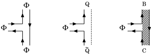
Figure 6: Vertices in the gauged matrix model.

Having found the Feynman rules, we can calculate the annulus contributions perturbatively. The annulus diagrams are drawn in Figures 7-9 up to three loops,.

Figure 7: The dump-bell diagram.

The contributions to annulus free energy from the dump-bell diagram Figure 7 is

$$\frac{S_{1}}{2g\Delta m^{2}}-\frac{S_{2}}{2g\Delta(m+\Delta)^{2}}.$$ (4.40)

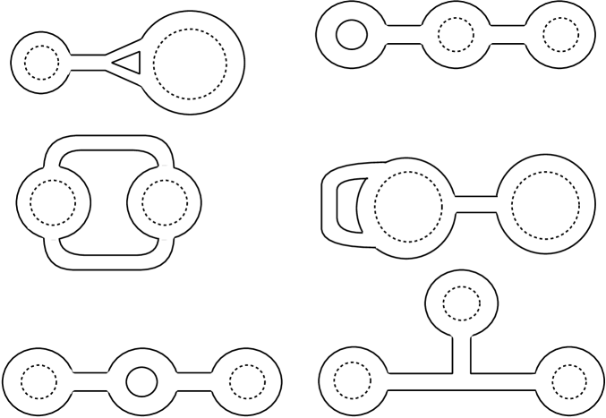
Figure 8: Three-loop diagrams contributing to $S_{1}^{2}$ or $S_{2}^{2}$.

Figure 9: Three-loop diagrams contributing to $S_{1}S_{2}$.

From the three-loop diagrams, we obtain the terms involving the $S_{1}^{2}$, $S_{2}^{2}$ and $S_{1}S_{2}$. The diagrams in Figure 8 lead to the $S_{1}^{2}$ and $S_{2}^{2}$ terms. We obtain the $S_{1}^{2}$ terms

$$\Bigl{[}-\frac{1}{g^{2}\Delta^{3}m^{3}}-\frac{1}{g^{2}\Delta^{3}m^{3}}+\frac{1}{4g^{2}\Delta^{2}m^{4}}+\frac{1}{g^{2}\Delta^{2}m^{4}}+\frac{1}{g^{2}\Delta^{4}m^{2}}+\frac{1}{g^{2}\Delta^{4}m^{2}}\Bigr{]}S_{1}^{2}.$$ (4.41)

The $S_{2}^{2}$ terms can be obtained by replacements $S_{1}\to S_{2}$, $\Delta\to-\Delta$ and $m\to m+\Delta$

$$\Bigl{[}\frac{1}{g^{2}\Delta^{3}(m+\Delta)^{3}}+\frac{1}{g^{2}\Delta^{3}(m+\Delta)^{3}}+\frac{1}{4g^{2}\Delta^{2}(m+\Delta)^{4}}+\frac{1}{g^{2}\Delta^{2}(m+\Delta)^{4}}$$

$$+\frac{1}{g^{2}\Delta^{4}(m+\Delta)^{2}}+\frac{1}{g^{2}\Delta^{4}(m+\Delta)^{2}}\Bigr{]}S_{2}^{2}.$$ (4.42)

Finally, the diagrams in Figure 9 lead to the $S_{1}S_{2}$ terms.

$$-\Biggl{[}\frac{1}{g^{2}\Delta^{4}}\left(\frac{1}{m^{2}}+\frac{1}{(m+\Delta)^{2}}\right)+\frac{2}{g^{2}\Delta^{4}}\left(\frac{1}{m^{2}}+\frac{1}{(m+\Delta)^{2}}\right)$$

$$\hskip 19.91684pt+\frac{2}{g^{2}\Delta^{3}}\left(-\frac{1}{m^{3}}+\frac{1}{(m+\Delta)^{3}}\right)+\frac{2}{g^{2}\Delta^{4}m(m+\Delta)}\Biggr{]}S_{1}S_{2}.$$ (4.43)

4.3.2 Comparison with the Annulus Formula

To compare these diagrammatic computation with the annulus formula (3.33), let us expand the latter in powers of $S_{1}$ and $S_{2}$. For the two-cut solution the prime form is defined on the curve

$$y^{2} = \left(\frac{1}{g}W^{\prime}(z)\right)^{2}+f_{1}(z)=(z-z_{1})(z-z_{2})(z-z_{3})(z-z_{4}),$$

$$W(z) = g\left(\frac{1}{3}z^{3}+\frac{\Delta}{2}z^{2}\right).$$ (4.44)

There are two 1-cycles : $A_{1}$ around $[z_{1},z_{2}]$ and $A_{2}$ around $[z_{3},z_{4}]$. We assume that the two cuts to be small so that we shall find a solution in a power series of the periods.

Using the addition theorem for the prime form, we write the annulus formula (3.33) on the curve (4.44) as

$$\frac{1}{2}\log\frac{E(m,\tilde{m})E(\tilde{\infty},\infty)}{E(m,\tilde{\infty})E(\tilde{m},\infty)}=\frac{1}{2}\int_{m}^{\infty}\omega_{\tilde{m}-\tilde{\infty}}.$$ (4.45)

The meromorphic 1-form $\omega_{\tilde{m}-\tilde{\infty}}$ on this curve is given by

$$\omega_{\tilde{m}-\tilde{\infty}}=\frac{1}{2}\left[\frac{dz}{z-m}\left(1-\frac{y(m)}{y(z)}\right)+\frac{(\alpha_{1}z+\alpha_{2})dz}{y(z)}\right].$$ (4.46)

The coefficients $\alpha_{1}$, $\alpha_{2}$ for the holomorphic forms are determined by the zero A-period conditions

$$\sum_{i=1}^{2}\oint_{A_{i}}\omega_{\tilde{m}-\tilde{\infty}}=0,$$

$$\oint_{A_{2}}\omega_{\tilde{m}-\tilde{\infty}}=0.$$

The integration in the first condition can be performed by deforming the contour to $A_{\infty}\cup(-{\cal C}_{m})$. As a result, we obtain $\alpha_{1}=1$. The integration in the second condition is rather difficult. To perform this integration, we introduce the parameterization [24]

$$z_{1}=\frac{Q-I}{2}-\Delta_{21},\quad z_{2}=\frac{Q-I}{2}+\Delta_{21},$$

$$z_{3}=\frac{Q+I}{2}-\Delta_{43},\quad z_{4}=\frac{Q+I}{2}+\Delta_{43},$$

$$Q:=\frac{z_{1}+z_{2}+z_{3}+z_{4}}{2},\quad I:=\frac{z_{3}+z_{4}}{2}-\frac{z_{1}+z_{2}}{2}.$$

By expanding the condition $\int_{z_{3}}^{z_{4}}\omega_{\tilde{m}-\tilde{\infty}}=0$ in terms of $\Delta_{21}$, we determine the coefficient $\alpha_{2}$ perturbatively up to ${\cal O}(\Delta_{21}^{4})$ as

$$\alpha_{2} = \sqrt{(m^{\prime}-z_{3})(m^{\prime}-z_{4})}+\frac{\Delta_{21}^{2}(z_{3}+z_{4})\biggl{(}-m^{\prime}+\sqrt{(m^{\prime}-z_{3})(m^{\prime}-z_{4})}\biggr{)}}{4z_{3}z_{4}m^{\prime}}$$

$$+\frac{\Delta_{21}^{4}}{128z_{3}^{3}z_{4}^{3}m^{\prime\;3}}\biggl{[}-m^{\prime\;2}\biggl{(}m^{\prime}+\sqrt{(m^{\prime}-z_{3})(m^{\prime}-z_{4})}\biggr{)}(z_{3}+z_{4})(9z_{3}^{2}-10z_{3}z_{4}+9z_{4}^{2})$$

$$+\sqrt{(m^{\prime}-z_{3})(m^{\prime}-z_{4})}\biggl{(}8z_{3}^{2}z_{4}^{2}(z_{3}+z_{4})+2z_{3}z_{4}m^{\prime}(3z_{3}^{2}+2z_{3}z_{4}+3z_{4}^{2})\biggr{)}\biggr{]}+{\cal O}(\Delta_{21}^{6}),$$

where $m^{\prime}:=m+\frac{I-Q}{2}$.

The periods of the curve (4.44)

$$S_{1}=g\int_{z_{3}}^{z_{4}}\frac{dz}{2\pi}\;y(z),\quad S_{2}=g\int_{z_{1}}^{z_{2}}\frac{dz}{2\pi}\;y(z)$$ (4.47)

are evaluated in terms of the variables $(Q,I,\Delta_{21},\Delta_{43})$. We can iteratively solve the inverse relations $\Delta_{21}(S_{1},S_{2},g,\Delta)$, $\Delta_{43}(S_{1},S_{2},g,\Delta)$ as [6]

$$\Delta_{43}(S_{1},S_{2},g,\Delta)^{2}=\frac{4}{g\Delta}S_{1}+\frac{8}{g^{2}\Delta^{4}}(2S_{1}^{2}-3S_{1}S_{2})+\frac{8}{g^{3}\Delta^{7}}S_{1}(5S_{1}-13S_{2})(4S_{1}-3S_{2})$$

$$\hskip 105.2751pt+{\cal O}(S^{4}),$$

$$\Delta_{21}(S_{1},S_{2},g,\Delta)^{2}=\Delta_{43}(S_{1},S_{2},g,-\Delta).$$ (4.48)

The integration of meromorphic 1-form (4.45) can be performed by expanding in terms of $\Delta_{21}$ and $\Delta_{43}$. By plugging the inverse relations (4.48), we obtain the perturbative expansion

$${\cal F}_{0}^{(2)} = \frac{S_{1}}{2g\Delta m^{2}}-\frac{S_{2}}{2g\Delta(m+\Delta)^{2}}$$ (4.49)

$$+\frac{5\Delta^{2}-8\Delta m+8m^{2}}{4g^{2}\Delta^{4}m^{4}}S_{1}^{2}+\frac{5\Delta^{2}+8\Delta m+8m^{2}}{4g^{2}\Delta^{4}(m+\Delta)^{4}}S_{2}^{2}$$

$$+\frac{2\Delta^{4}+3\Delta^{3}m-5\Delta^{2}m^{2}-16\Delta m^{3}-8m^{4}}{g^{2}\Delta^{4}m^{3}(m+\Delta)^{3}}S_{1}S_{2}+{\cal O}(S^{3}).$$

These terms precisely coincide with (4.41), (4.42) and (4.43). The absence of the contribution from $\omega^{(2)}(z)$ can also be checked to all orders by numerical calculations.

5 CFT Techniques

So far we have considered the planar contributions to the $\mbox{Tr}R\wedge R$ corrections in supersymmetric gauge theories. On the other hand, there are also corrections coming from the torus diagrams [39, 31, 40, 41], which are known to be elegantly computed using CFT techniques [42, 43, 5]. In this section we will see how the full $\mbox{Tr}R\wedge R$ correction ${\cal F}_{\chi=0}$ ($=$ the planar gravitational corrections ${\cal F}^{\mbox{\scriptsize(pl)}}$ (3.34) + the torus contribution ${\cal F}_{1}^{(0)}$) is reproduced in this framework for the gauge theories with matter. We will first recall how it works in the case without matter [44, 45, 46, 33], and then examine how the matter fields fit in the story.

5.1 CFT Techniques without Matter

Consider the matrix model partition function

$$Z = \int d\Phi\exp\left(-\frac{1}{g_{s}}{\rm Tr}W(\Phi)\right)$$ (5.1)

with an arbitrary tree level potential

$$W(\Phi)=-\sum_{k=0}^{\infty}t_{k}\Phi^{k}.$$ (5.2)

CFT techniques are based on the the equivalence of the loop equation and the Virasoro constraints [44, 45, 46, 33]. That is, defining the loop operator

$$\omega(z) := \frac{1}{\hat{N}}\mbox{Tr}\frac{1}{z-\Phi}$$ (5.3)

and the corrective field

$$\varphi(z) := -W(z)+2g_{s}\mbox{Tr}\log(z-\Phi),$$ (5.4)

$$\partial\varphi(z) = 2S\omega(z)-W^{\prime}(z),$$

the loop equation

$$\left<\omega(z)^{2}\right> = \frac{1}{g_{s}}\sum_{i=1}^{\hat{N}}\left<\frac{W^{\prime}(\lambda_{i})}{z-\lambda_{i}}\right>$$ (5.5)

can be written in the equivalent form

$$\left<\frac{1}{2\pi i}\oint_{C}dw\frac{(\partial\varphi(w))^{2}}{w-z}\right> = 0,$$ (5.6)

where $<\cdots>$ denotes the expectation value. Here the contour $C$ encircles all $w=\lambda_{i}$, the eigenvalues of $\Phi$, but not $w=z$. Since

$$\partial\varphi(z) = \sum_{n=0}^{\infty}nt_{n}z^{n-1}+\sum_{n=-\infty}^{-1}2g_{s}^{2}z^{n-1}\frac{\partial}{\partial t_{n}}$$

inside a correlator, $\varphi(z)$ may be regarded as a free chiral boson of conformal field theory [47], and the equation (5.5) can be written as the Virasoro constraints

$$\left<\oint_{C}dw\frac{T_{\mbox{\scriptsize em}}(w)}{w-z}\right> = 0,$$ (5.7)

where

$$T_{\mbox{\scriptsize em}}(z) = +\frac{1}{4g_{s}^{2}}(\partial\varphi(z))^{2}$$ (5.8)

is the energy-momentum tensor. Note that the prefactor $\frac{1}{4g_{s}^{2}}$ has been chosen so that their moments generate the Virasoro algebra in the standard normalization.

To leading order in $g_{s}$, $Z$ is computed by the saddle point approximation in which $\partial\varphi(z)$ is replaced with its large $\hat{N}$ expectation value $-y^{(0)}(z)$ [1]. We need to compute the next-to-leading order, which may be obtained by the Gaussian approximation around a classical solution [43], and hence is described by a free conformal field theory.

For the case of pure gauge theories without matter, CFT techniques were utilized [5] to compute the genus one contribution to the $\mbox{Tr}R\wedge R$ correction. This goes as follows: Consider the correlation function of $2n$ twist operators $\sigma(a_{i},\bar{a}_{i})$ $(i=1,\ldots,2n)$ on a sphere [48, 49, 50, 51, 52]

$$\left<\prod_{k=1}^{2n}\sigma(a_{k},\bar{a}_{k})\right>^{\rm\!\!CFT} = |\det A|^{-1}\prod_{i<j}^{2n}|a_{i}-a_{j}|^{-\frac{1}{4}}\sum_{(\{p_{i}\},\{\bar{p}_{i}\})}\exp\left[\frac{1}{2}i\pi(p\cdot\tau\cdot p-\bar{p}\cdot\bar{\tau}\cdot\bar{p})\right].$$

where $\tau$ is the period matrix of the double cover with genus $n$ (not $n\!-\!1$!; the extra handle arises by the plumbing fixture connecting $z=\infty$ and $\tilde{\infty}$. See Section 5.3.) and

$$A_{ij} := \oint_{A_{i}}dz\frac{z^{j-1}}{y}.~{}~{}~{}$$ (5.10)

The loop momenta $\{p_{i}\}_{i=1,\ldots,n-1}$ run over a certain momentum winding lattice.

It was argued in [43], and was recently confirmed in [40], that the genus one free energy can be built from the chiral determinant of a $c=1$ free boson CFT, or the chiral piece of (LABEL:A) with particular loop momenta

$$\left<\prod_{k=1}^{2n}\sigma(a_{k})\right>^{\rm\!\!CFT}_{p_{i}=-\sqrt{2}N_{i}} = e^{\pi iN\cdot\tau\cdot N}\mbox{det}\Delta_{0}^{-\frac{1}{2}}$$ (5.11)

$$= e^{\pi iN\cdot\tau\cdot N}\det A^{-\frac{1}{2}}\prod_{i<j}^{2n}(a_{i}-a_{j})^{-\frac{1}{8}}.$$

The important point is that the twist operator $\sigma(z)$ does not satisfy the Virasoro constraint (because, for example, it has nonzero conformal weight $\frac{1}{16}$) and hence must be replaced with an appropriately modified ‘star’ operator $S(z)$ [53] given by

$$S(z) = \mu_{\frac{3}{2}}(z)^{-\frac{1}{24}}\sigma(z),$$ (5.12)

$$<\partial\varphi(z)> = \sum_{r\geq\frac{1}{2}}\mu_{r}(a_{i})~{}(z-a_{i})^{r-1}$$ (5.13)

to this order of the approximation. If the number of cuts $n$ is equal to the degree of $W^{\prime}(\Phi)$, we find

$$\sum_{i=1}^{2n}\log\mu_{\frac{3}{2}}(a_{i}) = \log\prod_{i<j}(a_{i}-a_{j}),$$ (5.14)

The replacement (5.12) then correctly yields the genus one free energy

$$e^{{\cal F}^{\mbox{\scriptsize(pl)}}+{\cal F}_{1}^{(0)}} = \left<\prod_{k=1}^{2n}S(a_{k})\right>^{\rm\!\!CFT}_{p_{i}=-\sqrt{2}N_{i}}$$ (5.15)

$$= e^{\pi iN\cdot\tau\cdot N}\det A^{-\frac{1}{2}}\prod_{i<j}(a_{i}-a_{j})^{-\frac{1}{6}}$$

as was confirmed in [31, 40]. Note that the CFT result (5.15) also automatically includes the planar gravitational correction from sphere diagrams [16] with the momentum identification

$$p_{i} = -\sqrt{2}N_{i}~{}~{}~{}(i=1,\ldots,n).$$ (5.16)

5.2 The Full $\mbox{Tr}R\wedge R$ Correction and Fermion Correlators

We next consider the CFT interpretation of the gravitational corrections for gauge theories with matter. The partition function is now

$$Z = \int d\Phi\exp\left(-\frac{1}{g_{s}}{\rm Tr}W(\Phi)\right)e^{-\sum_{I=1}^{N_{f}}\mbox{\scriptsize Tr}\log(\Phi-m_{I})}.$$ (5.17)

Treating the second factor perturbatively, it is an expectation value of $e^{-\sum_{I=1}^{N_{f}}\mbox{\scriptsize Tr}\log(\Phi-m_{I})}$ with respect to the measure without matter. Since

$$\mbox{Tr}\log(\Phi-m_{I}) = \frac{1}{2g_{s}}(\varphi(m_{I})+W(m_{I}))+\mbox{Tr}\log(-1),$$ (5.18)

it should be obtained as a correlator of vertex operators charge $-\frac{1}{2g_{s}}$. If we take the convention that

$$<\varphi(z)\varphi(w)>^{\mbox{\scriptsize CFT}} \sim -\log(z-w),$$ (5.19)

the prefactor of (5.8) must be $-\frac{1}{2}$ so that $g_{s}^{2}=-\frac{1}{2}$. This motivates us to consider the CFT correlator

$$\left<\prod_{k=1}^{2n}\sigma(a_{k},\bar{a}_{k})\prod_{I=1}^{N_{f}}e^{\frac{1}{\sqrt{2}}i\varphi(m_{I})}\cdot e^{-\frac{N_{f}}{\sqrt{2}}i\varphi(\infty)}\right>^{\rm\!\!CFT}.$$ (5.20)

This is equivalent to a correlation function of conjugate pairs of the vertex operators on a hyper-elliptic Riemann surface without twist operators, except that their zero-mode contributions differ by a factor of two [52, 54]. In fact, to correctly reproduce the annulus amplitude we also need to take the normal ordering of the vertex operators on the same sheets :

$$\left<:\prod_{I=1}^{N_{f}}e^{\frac{1}{\sqrt{2}}i\varphi(m_{I})}\cdot e^{-\frac{N_{f}}{\sqrt{2}}i\varphi(\infty)}::\prod_{I=1}^{N_{f}}e^{-\frac{1}{\sqrt{2}}i\varphi(\tilde{m}_{I})}\cdot e^{\frac{N_{f}}{\sqrt{2}}i\varphi(\tilde{\infty})}:\right>^{\rm\!\!CFT}$$

$$\quad\quad\quad\quad=(\mbox{det}\Delta_{0})^{-1}\sum_{\scriptsize\begin{array}[]{c}(\{p_{i}\},\{\bar{p}_{i}\})\end{array}}A_{0}^{\{p_{i}\}}{\overline{A}_{0}^{\{p_{i}\}}},$$ (5.22)

where $A_{0}^{\{p_{i}\}}$ is the holomorphic block with loop momenta $\{p_{i}\}$ $(i=1,\ldots,n)$. Again, let us focus on a particular block of (5.22) with $p_{i}=-\sqrt{2}N_{i}$ $(i=1,\ldots,n)$. Taking the logarithm of this block, we have [52]

$$\log A_{0}^{\{-\sqrt{2}N_{i}\}} = 2\left(\pi i\sum_{i,j=1}^{n}\tau_{ij}N_{i}N_{j}+2\pi i\sum_{i=1}^{n}N_{i}\sum_{I=1}^{N_{f}}\int_{m_{I}}^{\infty}\hat{\omega}_{i}\right)$$ (5.23)

$$+\frac{1}{2}\sum_{I,J=1}^{N_{f}}\log\frac{E(m_{I},\tilde{\infty})E(\infty,\tilde{m}_{J})}{E(m_{I},\tilde{m}_{J})E(\infty,\tilde{\infty})}.$$

$\tau_{ij}$ is the period matrix of the Riemann surface on which the CFT is defined (See Section 5.3.). The first and second terms are twice of the planar gravitational corrections (3.35)(3.36). As we mentioned, the zero-mode part of the twist correlator is half of that on its double cover (eqs.(4.3) and (5.21) in [52]). The last term is equal to the annulus amplitude ${\cal F}_{0}^{(2)}$ (3.33); by definition of normal ordering, it does not contain the correlations between pairs of points on the same sheet. The ‘star’ization of the matter vertices is not necessary, since the contour $C$ in (5.7) does not encircle $z=m_{I}$. Thus we have shown that the chiral block (5.23) together with the corrected chiral determinant precisely reproduces all the contributions to the full $\mbox{Tr}R\wedge R$ correction for the gauge theories with matter.

Remarkably, the correlator (5.20) closely resembles that in the bosonization of fermions on Riemann surfaces [54]. This is in accord with the fact that the correlators of $\det(\Phi-m_{I})$ can be described as free fermion insertions in the soliton theory [55], and in some special case they are realized as CFT correlators [56]. However, a significant difference here is that they are all for the full matrix model correlators, whereas our result concerns only the contributions of ${\cal O}(1/\hat{N}^{2})$. Another important point is that the normal ordering is required in (5.22).

5.3 Non-compact Calabi-Yau as a Pinched Riemann Surface

The ${\cal N}=1$ supersymmetric gauge theories are realized in type IIB superstring theory on non-compact Calabi-Yau three-folds. If one computes the effective superpotential by using the geometric transition, one needs to introduce a cutoff $\Lambda_{0}$ to regularize some periods of a reduced non-compact Riemann surface. Although the quantities computed in matrix models are finite (since the eigenvalues are distributed on finite intervals), a cutoff is needed again if the free energy (or the disk amplitude) is written as a contour integral around infinity. Thus a matrix model curve with $n$ cuts is a genus $n-1$ punctured Riemann surface.

On the other hand, the CFT correlator formula obtained in [52] and used above assumes that the Riemann surface on which the CFT is defined is compact with no punctures. How can we understand the cutoff $\Lambda_{0}$ here? In fact, the Riemann surface for the CFT can be thought of as a pinched Riemann surface of genus $n$, where $|\Lambda_{0}/\Lambda|^{-2}$ is identified as the the pinching parameter $t$ of the plumbing fixture. Indeed, suppose that we identify two annular regions near $\infty$, $\tilde{\infty}$

$$W_{1} = \left\{p\in{\it\Sigma}^{g_{s}=0}_{n-1}\mbox{~{}on the 1st sheet}~{}\left|~{}|\Lambda|<|z(p)|<\left|\frac{\Lambda_{0}^{2}}{\Lambda}\right|\right.\right\},$$

$$W_{2} = \left\{p\in{\it\Sigma}^{g_{s}=0}_{n-1}\mbox{~{}on the 2nd sheet}~{}\left|~{}|\Lambda|<|z(p)|<\left|\frac{\Lambda_{0}^{2}}{\Lambda}\right|\right.\right\}$$ (5.24)

by gluing them with a cylinder

$$S = \{(X,Y)\in{\bf C}^{2}~{}|~{}XY=t\}$$ (5.25)

through the identification

$$(X,Y) = \left(\frac{|\Lambda|}{z},\frac{tz}{|\Lambda|}\right)\mbox{~{}~{}~{}for $W_{1}$},$$

$$(X,Y) = \left(\frac{tz}{|\Lambda|},\frac{|\Lambda|}{z}\right)\mbox{~{}~{}~{}for $W_{2}$}$$ (5.26)

with $\sqrt{t}=|\frac{\Lambda}{\Lambda_{0}}|$. Then $\hat{B}_{i}$’s $(i=1,\ldots,n)$ become closed contours, and we can verify by a change of the canonical homology basis that the period matrix $\{-\int_{\hat{B}_{i}}dz\;\hat{\omega}_{j}\}_{i,j=1,\ldots,n}$ coincides with Fay’s period matrix formula for the pinched Riemann surface [32] in the $|\Lambda_{0}|\rightarrow\infty$ limit.

6 On-shell Condition

6.1 The ${\cal N}=2$ Limit and the Torus Contribution

The ${\cal N}=2$ supersymmetry can be restored for $U(N)$ gauge theories if the superpotential is in the form

$$W(\phi)=g_{N+1}\left(\phi^{N+1}+\sum_{p=1}^{N}\frac{g_{p}}{p}\phi^{p}\right)$$ (6.1)

so that the gauge breaking pattern is $U(N)\to U(1)^{N}$; an ${\cal N}=2$ theory can be realized by taking the $g_{N+1}\rightarrow 0$ limit [25]. The Seiberg-Witten curve is recovered from the matrix model curve in this limit if the moduli $S_{i}$ satisfy the on-shell condition $\partial W_{\rm eff}(S_{i})/\partial S_{i}=0$ [17, 18]. (See also [57].) Turning off the superpotential term in this way, the ${\cal N}=1$ Weyl superfield $G_{\alpha\beta\gamma}(\theta)$ and the graviphoton superfield $F_{\alpha\beta}(\theta)$ are combined into a single ${\cal N}=2$ Weyl superfield $W_{\alpha\beta}(\theta,\psi)=F_{\alpha\beta}(\theta)+\psi^{\gamma}G_{\alpha\beta\gamma}$. Consequently, the ${\cal N}=1$ gravitational F-terms yield to an ${\cal N}=2$ F-term

$$\int d^{4}xd^{4}\theta{\cal F}_{\chi=0}({\cal S}_{i})W_{\alpha\beta}W^{\alpha\beta}.$$ (6.2)

One can thus recover the ${\cal N}=2$ results by simply replacing the matrix model curve with the Seiberg-Witten curve.

The $W^{2}$ factor contains the $\mbox{Tr}R\wedge R$ component; it can be calculated by topologically twisted ${\cal N}=2$ Yang-Mills theories [15], since the effect of the topological twist becomes invisible on a hyper-Kähler four-manifold $M_{4}$ and the coefficient of $\mbox{Tr}R\wedge R$ term of physical ${\cal N}=2$ theories agrees with that of topological theories. The latter yields up to a constant factor

$${\cal F}_{\chi=0}=b(S_{i})-\frac{2}{3}c(S_{i}),$$ (6.3)

$$b(S_{i})=-\frac{1}{2}\log\det A_{ij},\quad A_{ij}=\oint_{A_{i}}dz\frac{z^{j-1}}{y},$$

$$c(S_{i})=-\frac{1}{12}\log\Delta,\quad\Delta=\prod_{i<j}^{2N}(z_{i}-z_{j})^{2},$$

where $b(S_{i})$ and $c(S_{i})$ are defined on the Seiberg-Witten curve

$$y^{2}=P_{N}(z)^{2}-\Lambda^{2N-N_{f}}\prod_{I=1}^{N_{f}}(z-m_{I})=\prod_{i=1}^{2N}(z-z_{i}).$$ (6.4)

On the Seiberg-Witten curve, the torus free energy which is obtained by conformal field theory techniques exactly coincides with (6.3). Recently, it was confirmed that the topological partition function coincides with the multi-instanton counting formula [11] for $g=1$ [13]. Thus we find consistency of our formula with the ${\cal N}=2$ SYM results.

6.2 The Origin of the Planar Contributions?

We have, however, also the planar gravitational corrections, which have no counterpart in the instanton calculations of ${\cal N}=2$ theories. Where do these terms come from? A suggestive observation is that all the planar terms can be combined into a simple integral

$${\cal F}^{\mbox{\scriptsize(pl)}} = 2\pi i\left(\frac{1}{2}\sum_{i,j=1}^{n}N_{i}N_{j}\tau_{ij}+\sum_{i=1}^{n}N_{i}\sum_{I=1}^{N_{f}}\int_{m_{I}}^{\infty}\hat{\omega}_{i}\right)+\frac{1}{2}\sum_{I,J=1}^{N_{f}}\log\frac{E(m_{I},\tilde{\infty})E(\infty,\tilde{m}_{J})}{E(m_{I},\tilde{m}_{J})E(\infty,\tilde{\infty})}$$ (6.5)

$$= -\pi i\left(\sum_{i=1}^{n}N_{i}\int_{\hat{B}_{i}}-\sum_{I=1}^{N_{f}}\int_{m_{I}}^{\infty}\right)dz\;T(z),$$

where

$$T(z)\;dz = \sum_{i=1}^{n}N_{i}\hat{\omega}_{i}+\frac{1}{2\pi i}\sum_{I=1}^{N_{f}}\omega_{\tilde{m_{I}}-\tilde{\infty}}$$ (6.6)

is nothing but the gauge theory expectation value of $\left<\mbox{Tr}\frac{1}{z-\phi}\right>$ and solves the Konishi anomaly equations [18]! Since the B-period integrals of $T(z)$ on shell may naturally be regarded as NS-NS fluxes on a deformed Calabi-Yau three-fold [24]

$$W^{\prime}(z)^{2}+f_{n-1}(z)+y^{2}+v^{2}+w^{2}=0,\quad(z,y,v,w)\in\bf{C}^{4},$$ (6.7)

it suggests that ${\cal F}^{\mbox{\scriptsize(pl)}}$ would correspond to some interaction term on the D5-branes couple to 2-form field $B_{2}=B_{R}+\tau B_{NS}$ before the geometric transition. This motivates us to consider the induced Chern-Simons term on D$p$-branes [58]

$$I=\int_{M_{p+1}}C\wedge{\rm ch}(F)\wedge\sqrt{\hat{A}(R)},$$ (6.8)

where $C$ is a form field on the D$p$-branes. ${\rm ch}(F)$ and $\hat{A}(R)$ are defined for the Chan-Paton gauge and tangent bundles on $M_{p+1}$, respectively. In our case D5-branes are wrapped around 2-cycles in a Calabi-Yau three-fold and filling the four-dimensional space-time. From this Chern-Simons term we obtain the $\mbox{Tr}R\wedge R$ term

$$\int_{M_{6}}C\wedge({\rm tr}{\bf 1})\mbox{Tr}R\wedge R,$$ (6.9)

where ${\rm tr}{\bf 1}$ comes from ${\rm ch}(F)$ and $C$ is restricted to a 2-form in the Calabi-Yau direction. In this brane setup we will have the $\mbox{Tr}R\wedge R$ term

$$\left(\sum_{i=1}^{n}N_{i}\int_{\hat{B}_{i}}+\sum_{I=1}^{N_{f}}\int_{\tilde{m}_{I}}^{\tilde{\infty}}\right)B_{\rm NS}\int_{\bf{R}^{4}}\mbox{Tr}R\wedge R.$$ (6.10)

Note that the weight factors $N_{i}$ naturally arise from ${\rm tr}{\bf 1}$. Thus, we conjecture that the on-shell planar gravitational corrections may have their origin in the Chern-Simons coupling induced on the D5-branes.

Although these arguments are not conclusive, the relation (6.5) is certainly suggestive and would be worth being studied.

7 Summary and Discussion

In this paper we have studied the gravitational corrections to the effective superpotential in four-dimensional ${\cal N}=1$ $U(N)$ gauge theories with flavors in the fundamental representation, using the matrix model approach of Dijkgraaf and Vafa. We derived a compact formula for the annulus contribution to the corrections in terms of the prime form on the matrix model curve. We also showed that the full $\mbox{Tr}R\wedge R$ correction containing the torus as well as all the planar contributions can be reproduced as a special momentum sector of a single $c=1$ CFT correlator. The ${\cal N}=2$ limit of the torus contribution agrees with the answer of the multi-instanton calculations and also with the geometric engineering argument from the topological A-model. The planar contributions, on the other hand, have no counterpart in the instanton calculations of ${\cal N}=2$ gauge theories, and we speculated that the latter might correspond to the Chern-Simons term induced on the D5-branes.

The CFT correlator we found is very close to the fermion correlator on the Riemann surface. In [22] the correspondence between the non-compact B-branes and fermions has been discussed. Since the matter contributions come from the $N_{f}$ D5-branes wrapped around non-compact 2-cycles, our result is consistent with the picture [22, 23]. In the topological B-model, the genus one partition function is given by a generalized holomorphic Ray-Singer torsion on the Calabi-Yau geometry [28]

$${\cal F}_{1}=\sum_{p,q=1}^{3}pq(-1)^{p+q}\log\det\Delta_{p,q},$$ (7.1)

where $\Delta_{p,q}$ is the Laplacian acting on $(p,q)$-forms. By using Quillen’s anomaly, we also find the one-loop open topological string partition function. Our formula may lead to the explicit expression for it on a non-compact Calabi-Yau three-fold.

There are various interesting directions to extend our analysis carried out in this paper. A simple extension of our analysis will be to investigate the gravitational corrections to the $SO/Sp$ gauge theories. If the ${\cal N}=2$ theory is deformed by an adjoint chiral superfield, the Chern-Simons coupling term is also induced by the orientifold plane [59]. It would be interesting to see whether such terms arise from the Klein bottle amplitudes in orthogonal matrix models. On the other hand, real symmetric/symplectic matrix models describe non-perturbative aspects of the $SO/Sp$ gauge theories with flavors in the symmetric/antisymmetric tensor representations, respectively. The CFT description of these matrix models can be given by a $c=-2$ CFT [60]. We will report on this elsewhere.

Another interesting issue to consider concerns higher dimensional gauge theories. It was proposed in [61, 62] that some five dimensional gauge theories can be described by unitary matrix models. The associated matrix model curve is represented by a pair of cylinders, where $z=+\infty$ and $-\infty$ cannot be distinguished. As a result there exist two chiral boson fields in the CFT description. It is interesting to investigate whether the five dimensional multi-instanton calculations can be reproduced in this CFT analysis. We also expect that the meaning of the five dimensional Chern-Simons term [14, 62] will be clarified.

Acknowledgements: We would like to thank M. Naka for his collaboration at an early stage of this work, and N. Ishibashi and H. Kanno for useful discussions. We also thank H. Eguchi, T. Eguchi, S. Hosono, S. Iso, K. Ito, M. Jinzenji, A. Kato, H. Kawai, T. Kawai, Y. Kitazawa, Y. Matsuo, Y. Nakayama, M. Natsuume, Y. Ookouchi, H. Suzuki, Y. Sugawara, Y. Tachikawa, Y. Yamada and A. Yamaguchi for helpful comments. The research of S.M. was supported in part by Grant-in-Aid for Scientific Research (C)(2) #14540286 from Ministry of Education, Culture, Sports, Science and Technology.

Appendix A  

In this Appendix we give an alternative proof of (3.17). See Section 3.3 for the definitions of $\omega^{(2)}(z)$, $y^{(2)}(z)$, etc.

A.1 Singularities of $\omega^{(2)}(z)dz$

We will first determine $\omega^{(2)}(z)dz$ from its singularities. In fact, to prove the assertion, the precise form is not needed. We will nevertheless derive it for future convenience for it is relevant to the computation of ${\cal F}_{0}^{(3)}$.

First of all, $\omega^{(2)}(z)dz$ (as well as other higher $\omega^{(k)}(z)dz$’s for all $k\geq 1$) has zero A-periods, for the same reason as before —— $S_{i}$’s are independent of $g_{s}$. In fact, $\omega^{(2)}(z)dz$ has only singularities at the $2n$ branch points $z=a_{i}(0)$ $(i=1,\ldots,2n)$, which are of second order. They arise since the matter insertions change the locations of the cuts. We will show that $\omega^{(2)}(z)dz$ is an abelian differential of the second kind with zero A-periods and given by

$$\omega^{(2)}(z) = \frac{1}{\sqrt{\prod_{l=1}^{2n}(z-a_{l})}}\sum_{i=1}^{2n}\frac{{a^{\prime}_{i}}^{2}M_{i}^{(1)}\prod_{\scriptsize\begin{array}[]{c}k\!\!=\!\!1\\ k\!\!\neq\!\!i\end{array}}^{2n}(a_{i}-a_{k})}{16S(z-a_{i})}+\frac{\sum_{j=0}^{n-2}p_{j}z^{j}}{\sqrt{\prod_{l=1}^{2n}(z-a_{l})}}$$ (A.3)

for some $p_{j}$ $(j=0,\ldots,n-2)$, where $a_{i}:=a_{i}(0)$, $a^{\prime}_{i}:=a^{\prime}_{i}(0)$ and

$$M_{i}^{(1)} = \frac{1}{2\pi i}\oint_{A_{\infty}}dz\frac{W^{\prime}(z)}{(z-a_{i})\sqrt{\prod_{l=1}^{2n}(z-a_{l})}}~{}~{}~{}(i=1,\ldots,2n).$$ (A.4)

$M_{i}^{(1)}$’s are the moments introduced in [31]. $p_{j}$’s $(j=0,\ldots,n-2)$ are determined so that $\omega^{(2)}(z)$ has zero A-periods.

Instead of studying the singularities of $\omega(z,g_{s})$ directly, it is easier to investigate those of $y(z,g_{s})$ (LABEL:yzgs). $y^{(2)}(z)$ and $-2S\omega^{(2)}(z)$ have the same singularities since the difference between the two is only linear in $g_{s}$.

It is easy to see that $y^{(2)}(z)dz$ is regular at $z=m_{I}$, $\tilde{m}_{I}$ $(I=1,\ldots,N_{f})$ since $\sum_{I}\frac{g_{s}}{z-m_{I}}$ has no singularity of ${\cal O}(g_{s}^{2})$. The integral representation (LABEL:yzgs) shows that $y^{(2)}(z)dz$ has possible singularities at $z=\infty$, $\tilde{\infty}$ and the branch points $z=a_{j}(0)$ ($j=1,\ldots,2n$). However, using the conditions (3.22) as well as those obtained by acting $\frac{\partial}{\partial g_{s}}|_{g_{s}=0}$ and $\frac{\partial^{2}}{\partial g_{s}^{2}}|_{g_{s}=0}$, it can be shown that the singularities at $z=\infty$, $\tilde{\infty}$ precisely cancel. Therefore, we have only to examine the singular behavior of $y^{(2)}(z)$ at the branch points.

Since

$$y^{(2)}(z) = \frac{1}{2}\left.\frac{\partial^{2}y(z,g_{s})}{\partial g_{s}^{2}}\right|_{g_{s}=0},$$ (A.5)

we see that the singularities at the branch points arise when $\left.\frac{\partial^{2}}{\partial g_{s}^{2}}\right|_{g_{s}=0}$ acts on the first factor $\sqrt{\prod_{i=1}^{2n}(z-a_{i}(g_{s}))}$ of $y(z,g_{s})$, and therefore $y^{(2)}(z)$ is proportional to

$$\frac{1}{2\pi i}\left(\oint_{C}+\oint_{C_{z}}\right)dw\left.\frac{W^{\prime}(w)+\sum_{I=1}^{N_{f}}\frac{g_{s}}{w-m_{I}}}{(z-w)\sqrt{\prod_{i=1}^{2n}(w-a_{i}(g_{s}))}}\right|_{g_{s}=0}$$

$$~{}~{}~{}~{}~{}~{}~{}~{}~{}~{}~{}~{}=\frac{1}{2\pi i}\oint_{A_{\infty}}dw\frac{W^{\prime}(w)}{(z-w)\sqrt{\prod_{i=1}^{2n}(w-a_{i}(0))}}$$

$$~{}~{}~{}~{}~{}~{}~{}~{}~{}~{}~{}\stackrel{{\scriptstyle z\rightarrow a_{j}}}{{\longrightarrow}}~{}-M_{j}^{(1)}~{}~{}~{}(j=1,\ldots,2n).$$ (A.6)

The contour $C$ surrounds all the cuts, and $C_{z}$ surrounds $w=z$. Matching the Laurent coefficients at the branch points, we obtain

$$y^{(2)}(z) = -\frac{1}{\sqrt{\prod_{l=1}^{2n}(z-a_{l})}}\sum_{i=1}^{2n}\frac{{a^{\prime}_{i}}^{2}M_{i}^{(1)}}{8(z-a_{i})}\prod_{\scriptsize\begin{array}[]{c}k\!\!=\!\!1\\ k\!\!\neq\!\!i\end{array}}^{2n}(a_{i}-a_{k})+\mbox{holomorphic differentials}.$$ (A.9)

This implies the equation (A.3).

Unlike $\omega^{(1)}(z)$, $\omega^{(2)}(z)$ depends on the potential $W(\Phi)$ not only through the positions of the cut but also through the moments $M_{i}^{(1)}$, reflecting the non-universality of ${\cal F}^{(3)}_{0}$.

A.2 An Alternative Proof of (3.17)

We will now prove (3.17). Using the saddle point equation

$$\frac{\partial W(\lambda,g_{s})}{\partial\lambda} = 2S\int_{-\infty}^{\infty}d\lambda^{\prime}\frac{\rho(\lambda^{\prime},g_{s})}{\lambda-\lambda^{\prime}},$$ (A.11)

the large $\hat{N}$ free energy (3.25) is written as

$${\cal F}_{0}(g_{s})=\sum_{j=1}^{n}S_{j}\left(\int_{-\infty}^{\infty}d\lambda\rho(\lambda,g_{s})\left(-\frac{1}{2}W(\lambda,g_{s})+S\log\frac{|\lambda-\lambda_{0j}|}{\Lambda}\right)-\frac{1}{2}W(\lambda_{0j},g_{s})\right).$$ (A.12)

Note that (A.11) is true only if $\lambda$ belongs to the nonzero support of $\rho(\lambda,g_{s})$, that is, only if $\lambda$ is such that $\rho(\lambda,g_{s})\neq 0$. $\lambda_{0j}$ is an arbitrary point on the $j$-th cut, whose location is independent of $g_{s}$.

We can extract the annulus contribution

$${\cal F}_{0}^{(2)} = {\cal F}_{0}^{(2)}({\bf I})+{\cal F}_{0}^{(2)}({\bf II}),$$ (A.13)

$${\cal F}_{0}^{(2)}({\bf I}) := -\frac{S}{2}\int_{-\infty}^{\infty}d\lambda\rho^{(1)}(\lambda)\sum_{I=1}^{N_{f}}\log(\lambda-m_{I}),$$

$${\cal F}_{0}^{(2)}({\bf II}) := -\sum_{j=1}^{n}\frac{S_{j}}{2}\int_{-\infty}^{\infty}d\lambda\rho^{(2)}(\lambda)\left(W(\lambda)-2S\log|\lambda-\lambda_{0j}|\rule{0.0pt}{11.38109pt}\right).$$ (A.14)

($\log\Lambda$ drops out since $\int_{-\infty}^{\infty}d\lambda\rho^{(2)}(\lambda)=0$.) Since ${\cal F}_{0}^{(2)}({\bf I})$ is already the right hand side of (3.17), we must show that ${\cal F}_{0}^{(2)}({\bf II})=0$. For this purpose let us first rewrite (A.14) in a contour integral on the first sheet using $\omega^{(2)}(z)$. We take the branch cut of $\log(z-\lambda_{0j})$ so that it runs from $z=\lambda+i0$ ($z=\lambda$ on the upper side of the cut)to $z=-\infty$. Then depending on $i<j$, $=j$ or $>j$ we have

$$\int_{a_{2i-1}}^{a_{2i}}d\lambda\rho^{(2)}(\lambda)\log|\lambda-\lambda_{0j}|$$

$$=\left\{\begin{array}[]{ll}{\displaystyle\frac{1}{2\pi i}\int_{A_{i}}dz\;\omega^{(2)}(z)\left(\log(z-\lambda_{0j})+\pi i\right)}&(i<j),\\ {\displaystyle\frac{1}{2\pi i}\left(\int_{A_{j}(\lambda_{0j})}dz\;\omega^{(2)}(z)\log(z-\lambda_{0j})+\pi i\int_{\lambda_{0j}+i0}^{\lambda_{0j}-i0}dz\;\omega^{(2)}(z)\right)}&(i=j),\\ {\displaystyle\frac{1}{2\pi i}\int_{A_{i}}dz\;\omega^{(2)}(z)\log(z-\lambda_{0j})}&(i>j),\end{array}\right.$$ (A.18)

where the contour $A_{j}(\lambda_{0j})$ starts from $z=\lambda_{0j}+i0$, surrounds the $j$th cut once anti-clockwise and goes back to $z=\lambda_{0j}+i0$ again but on the other side of the branch cut of $\log(z-\lambda_{0j})$. From (A.18) we find

$$\int_{-\infty}^{\infty}d\lambda\rho^{(2)}(\lambda)\log|\lambda-\lambda_{0j}| = \frac{1}{4S}\lim_{|\Lambda_{0}|\rightarrow\infty}\int_{\hat{B}_{j}}dz\;y^{(2)}(z)~{}~{}~{}(j=1,\ldots,n).$$ (A.19)

Therefore, to prove $F_{0}^{(2)}({\bf II})=0$ it suffices to show that

$$\frac{1}{2\pi i}\sum_{j=1}^{n}\oint_{A_{j}}\!\!dz\;y^{(2)}(z)W(z)+\sum_{j=1}^{n}S_{j}\!\!\oint_{B_{j}}dz\;y^{(2)}(z) = 0.$$ (A.20)

This can be proved by applying Riemann’s bilinear identity, as we will show below.

Cut out along

$$A_{n-1}B_{n-1}A_{n-1}^{-1}B_{n-1}^{-1}\cdots A_{1}B_{1}A_{1}^{-1}B_{1}^{-1},$$ (A.21)

${\it\Sigma}^{g_{s}}_{n-1}$ is represented by a $4(n-1)$-sided polygon with identification in a standard manner. Since $y^{(2)}(z)dz$ is an abelian differential of the second kind, its integral

$$Y(z):=\int_{z_{0}}^{z}dx\;y^{(2)}(x)$$ (A.22)

defines a single-valued meromorphic function $Y(z)$ inside the polygon for an arbitrary reference point $z_{0}$. Let us evaluate the integral of

$$\eta:=Y(z)y^{(0)}(z)dz$$ (A.23)

along the $4(n-1)$ sides of the polygon. Applying Riemann’s bilinear identity, we obtain

$$2\pi i\sum_{p\in{\it\Sigma}^{g_{s}}_{n-1}}\mbox{Res}_{p}\eta = \sum_{j=1}^{n-1}\left(\oint_{A_{j}}\!\!dzy^{(2)}(z)\oint_{B_{j}}\!\!dxy^{(0)}(x)-\oint_{B_{j}}\!\!dzy^{(2)}(z)\oint_{A_{j}}\!\!dxy^{(0)}(x)\right).$$

The right hand side is

right hand side of (LABEL:identity) $$= 4\pi i\sum_{j=1}^{n-1}S_{j}\oint_{B_{j}}\!\!dz\;y^{(2)}(z).$$ (A.25)

Let us compute the left hand side. Since

$$y^{(0)}(z) \stackrel{{\scriptstyle z\rightarrow\infty}}{{\rightarrow}} -\frac{2S}{z}+W^{\prime}(z)+{\cal O}(z^{-2}),$$ (A.26)

$$\stackrel{{\scriptstyle z\rightarrow\tilde{\infty}}}{{\rightarrow}} +\frac{2S}{z}-W^{\prime}(z)+{\cal O}(z^{-2}),$$

we find

$$2\pi i\mbox{Res}_{\infty}\eta = \oint_{A_{\infty}}dz\;y^{(2)}(z)W(z)+4\pi iSY(\infty),$$

$$2\pi i\mbox{Res}_{\tilde{\infty}}\eta = -\oint_{A_{\tilde{\infty}}}dz\;y^{(2)}(z)W(z)-4\pi iSY(\tilde{\infty})$$ (A.27)

$$= +\oint_{A_{\infty}}dz\;y^{(2)}(z)W(z)-4\pi iSY(\tilde{\infty}),$$

where $A_{\tilde{\infty}}$ is the same as $A_{\infty}$ but on the second sheet. We have shown in section A.1 that $y^{(2)}(z)dz$ has second order poles at every branch point $z=a_{i}$ $(i=1,\ldots,2n)$, and therefore $Y(z)$ has first order poles there, while we also see from (LABEL:yzgs) that $y^{(0)}dz$ has first order zeroes at those branch points. Therefore $\eta$ is regular there and hence has no nonzero residues. Thus, in all, we have

$$\mbox{left hand side of (\ref{identity})}=2\oint_{A_{\infty}}dz\;y^{(2)}(z)W(z)+4\pi iS\left(Y(\infty)-Y(\tilde{\infty})\right).$$ (A.28)

By definition

$$Y(\infty)-Y(\tilde{\infty}) = \int^{\infty}_{\tilde{\infty}}dz\;y^{(2)}(z),$$ (A.29)

where the contour cannot cross any side of the polygonal region since $Y(z)$ is single-valued only inside. Therefore the contour can pass only through the $n$th cut:

$$Y(\infty)-Y(\tilde{\infty}) = \lim_{|\Lambda_{0}|\rightarrow\infty}\int_{\hat{B}_{n}}dz\;y^{(2)}(z).$$ (A.30)

Plugging (A.30) into (A.28) and equating it with (A.25), we obtain the desired equation (A.20).

Appendix B  The Special Geometry Relation

It is now well-known that the sphere amplitude ${\cal F}_{0}^{(0)}$ satisfies the special geometry relation

$$\frac{\partial{\cal F}_{0}^{(0)}}{\partial S_{i}} = \lim_{|\Lambda_{0}|\rightarrow\infty}\left(\frac{1}{2}\int_{\hat{B}_{i}}dz\;y^{(0)}(z)-W(\Lambda_{0})+2S\log\frac{-\Lambda_{0}}{\Lambda}\right).$$ (B.1)

This fact was pointed out and proven using the energy cost argument in [1]. A proof using a Legendre transformation was given in [18]. In this Appendix we will give a sketch of an alternative proof neither using Legendre transformations nor resorting to any physical argument.

Before we consider (B.1), we first recall the relation [36]

$$\frac{\partial y^{(0)}(z)}{\partial S_{i}}dz = -4\pi i\hat{\omega}_{i}(z)~{}~{}~{}(i=1,\ldots,n),$$ (B.2)

where, as we defined in the text, $y^{(0)}(z)$ is related to the large $\hat{N}$ resolvent $\omega^{(0)}(z)$ by

$$y^{(0)}(z) = W^{\prime}(z)-2S\omega^{(0)}(z).$$ (B.3)

Note that the relation (B.2) is also true when the degree of $W^{\prime}(z)$ exceeds the number of the cut $n$ and $y^{(0)}(z)$ has extra zero factors (See footnote 3.). To see this we first use the integral representation of $y^{(0)}(z)$ (obtained by setting $g_{s}=0$ in (LABEL:yzgs)) to verify that the possible singularities of $\frac{\partial y^{(0)}(z)}{\partial S_{i}}$ are only located at $z=\infty$ and $\tilde{\infty}$. Next we write

$$y^{(0)}(z) =\sqrt{W^{\prime}(z)^{2}+f(z,\{S_{j}\})}$$ (B.4)

for some $f(z,\{S_{j}\})$ to find that

$$\frac{f(z,\{S_{j}\})}{W^{\prime}(z)} \stackrel{{\scriptstyle z\rightarrow\infty}}{{\rightarrow}} {\cal O}(\frac{1}{z})$$ (B.5)

since

$$2S\omega^{(0)}(z) = W^{\prime}(z)-\sqrt{W^{\prime}(z)^{2}+f(z,\{S_{j}\})}$$ (B.6)

$$= \frac{-f(z,\{S_{j}\})}{W^{\prime}(z)+\sqrt{W^{\prime}(z)^{2}+f(z,\{S_{j}\})}}$$

must behave like $\frac{2S}{z}+{\cal O}(\frac{1}{z^{2}})$ as $z\rightarrow\infty$. Therefore we find that

$$\frac{\partial y^{(0)}}{\partial S_{i}}dz = \frac{\frac{\partial}{\partial S_{i}}f(z,\{S_{j}\})}{2\sqrt{W^{\prime}(z)^{2}+f(z,\{S_{j}\})}}dz$$ (B.7)

has at most a first order pole at $z=\infty$, and hence can be written as a linear combination of $\hat{\omega}_{i}$’s. Then (B.2) follows from the fact that the $A_{i}$-period of $y^{(0)}(z)dz$ is $-4\pi iS_{i}$ $(i=1,\ldots,n)$.

We will now prove the special geometry relation (B.1). ${\cal F}_{0}^{(0)}$ is given by

$${\cal F}_{0}^{(0)} = -\frac{S}{2}\int_{-\infty}^{\infty}d\lambda\rho^{(0)}(\lambda)W(\lambda)$$ (B.9)

$$+S\sum_{j=1}^{n}S_{j}\left(\int_{-\infty}^{\infty}d\lambda\rho^{(0)}(\lambda)\log\frac{|\lambda-\lambda_{0j}|}{\Lambda}-\frac{1}{2S}W(\lambda_{0j})\right).$$

We express it in terms of contour integrals of the complex plane. Note that the integral of $dzy^{(0)}(z)\log(z-\lambda_{0j})$ along $A_{\infty}$ does not vanish as $|\Lambda_{0}|\rightarrow\infty$, and hence must be taken into account:

$${\cal F}_{0}^{(0)} = \lim_{|\Lambda_{0}|\rightarrow\infty}\left[\rule{0.0pt}{19.91692pt}\frac{1}{8\pi i}\oint_{A_{\infty}}dz\;y^{(0)}(z)W(z)\right.$$ (B.10)

$$~{}~{}~{}~{}~{}~{}\left.+\sum_{j=1}^{n}\frac{S_{j}}{4}\int_{\hat{B}_{j}}dz\;y^{(0)}(z)-\frac{S}{2}W(\Lambda_{0})+S^{2}\log\frac{-\Lambda_{0}}{\Lambda}\right].$$

Differentiating it by $S_{i}$, we find

$$\frac{\partial{\cal F}_{0}^{(0)}}{\partial S_{j}} = \lim_{|\Lambda_{0}|\rightarrow\infty}\left[-\frac{1}{2}\oint_{A_{\infty}}\hat{\omega}_{i}(z)W(z)-\pi i\sum_{j=1}^{n}S_{j}\int_{\hat{B}_{j}}\hat{\omega}_{i}(z)+S\log\frac{-\Lambda_{0}}{\Lambda}\right.$$ (B.11)

$$~{}~{}~{}~{}~{}~{}~{}\left.+\frac{1}{4}\int_{\hat{B}_{j}}dz\;y^{(0)}(z)-\frac{1}{2}W(\Lambda_{0})+S\log\frac{-\Lambda_{0}}{\Lambda}\right],$$

where the $S\log\Lambda_{0}$ terms are separated so that each line gives a finite result. Again, we can simplify it by using Riemann’s bilinear relation. In this case we cut out the Riemann surface along

$$A_{n-1}B_{n-1}A_{n-1}^{-1}B_{n-1}^{-1}\cdots A_{1}B_{1}A_{1}^{-1}B_{1}^{-1}A_{\tilde{\infty}}\hat{B}_{n}A_{\infty}(\hat{B}_{n})^{-1}$$ (B.12)

and evaluate

$$\int dz\;y^{(0)}(z)\Omega_{i}(z),~{}~{}~{}\Omega_{i}(z):=\int_{z_{0}}^{z}\omega_{i}(x)~{}~{}~{}(i=1,\ldots,n),~{}~{}~{}\omega_{n}(z):=\hat{\omega}_{n}(z)$$ (B.13)

along the boundary of the resulting polygon. The result we obtain is

$$\lim_{|\Lambda_{0}|\rightarrow\infty}\left[\oint_{A_{\infty}}\hat{\omega}_{i}(z)W(z)+2\pi i\sum_{j=1}^{n}S_{j}\int_{\hat{B}_{j}}\hat{\omega}_{i}(z)+\frac{1}{2}\int_{\hat{B}_{i}}dz\;y^{(0)}(z)-W(\Lambda_{0})\right]=0$$ (B.14)

for $i=1,\ldots,n$. Using (B.14) in (B.11), we obtain the special geometry relation (B.1).

Appendix C  The Large $\hat{N}$ Free Energy for a Quadratic Potential

$${\cal F}_{0} = \frac{S}{2}\left[\frac{t^{2}\mu(g_{s})^{2}}{S}\left(\frac{c(g_{s})^{2}}{2}+\frac{\mu(g_{s})^{2}}{8}\right)\right.$$ (C.1)

$$-\frac{\frac{g_{s}t}{S}}{\alpha(g_{s})-\alpha(g_{s})^{-1}}\left(\frac{\mu(g_{s})(m+c(g_{s}))}{2}-\frac{m^{2}}{\alpha(g_{s})}\right)$$

$$-\frac{g_{s}t\mu(g_{s})^{2}}{2S}\left(\log\left(-\frac{\mu(g_{s})\alpha(g_{s})}{2}\right)+\frac{1}{2\alpha(g_{s})^{2}}\right)$$

$$-\frac{g_{s}^{2}}{S}\left(\frac{\alpha(g_{s})^{-1}(\log(-\frac{\mu(g_{s})}{2})-1)+\alpha(g_{s})\log\alpha(g_{s})}{\alpha(g_{s})-\alpha(g_{s})^{-1}}-\log(\alpha(g_{s})-\alpha(g_{s})^{-1})\right)$$

$$+t\mu(g_{s})^{2}\left(\log\frac{\mu(g_{s})}{2}+\frac{c(g_{s})^{2}}{\mu(g_{s})^{2}}-\frac{1}{2}\right)$$

$$+2g_{s}\left(\frac{\frac{m-c(g_{s})}{\mu(g_{s})}\log\frac{\mu(g_{s})}{2}+\frac{c(g_{s})}{\mu(g_{s})}}{\alpha(g_{s})-\alpha(g_{s})^{-1}}-\frac{1}{2}\log\frac{m}{\alpha(g_{s})}\right)$$

$$\left.\rule{0.0pt}{17.07164pt}+g_{s}\log(-m)\right],$$

where

$$\alpha(g_{s})^{\pm 1} = \frac{m-c(g_{s})\pm\sqrt{(m-c(g_{s}))^{2}-\mu(g_{s})^{2}}}{\mu(g_{s})}.$$ (C.2)

References

- [1] R. Dijkgraaf and C. Vafa, Nucl. Phys. B644 (2002) 3 [hep-th/0206255]; Nucl. Phys. B644 (2002) 21 [hep-th/0207106]; [hep-th/0208048].
- [2] F. Cachazo, N. Seiberg and E. Witten, JHEP 0302 (2003) 042 [hep-th/0301006]
-
[3]
F. Cachazo, M. R. Douglas, N. Seiberg and E. Witten,
JHEP 0212 (2002) 071 [hep-th/0211170].
N. Seiberg, JHEP 0301 (2003) 061 [hep-th/0212225]. -
[4]
H. Kawai, T. Kuroki and T. Morita,
Nucl. Phys. B664 (2003) 185 [hep-th/0303210],
Nucl. Phys. B683 (2004) 27 [hep-th/0312026].
T. Morita, [hep-th/0403259]. - [5] R. Dijkgraaf, A. Sinkovics and M. Temurhan [hep-th/0211241].
- [6] A. Klemm, M. Marino and S. Theisen, JHEP 0303 (2003) 051 [hep-th/0211216].
- [7] H. Ooguri and C. Vafa, Adv. Theor. Math. Phys. 7 (2003) 53 [hep-th/0302109]; Adv. Theor. Math. Phys. 7 (2004) 405 [hep-th/0303063].
-
[8]
J. R. David, E. Gava and K.S. Narain,
JHEP 0309 (2003) 043 [hep-th/0304227].
L. F. Alday, M. Cirafici, J. R. David, E. Gava and K.S. Narain, JHEP 0401 (2004) 001 [hep-th/0305217].
L. F. Alday and M. Cirafici, JHEP 0309 (2003) 031 [hep-th/0306299].
J. R. David, E. Gava and K.S. Narain, JHEP 0309 (2003) 043 [hep-th/0311086]. -
[9]
H. Ita, H. Nieder and Y. Oz,
JHEP 0312 (2003) 046 [hep-th/0309041].
B. M. Gripaios, [hep-th/0311025]. - [10] S. Chiantese, A. Klemm and I. Runkel, JHEP 0403 (2004) 033 [hep-th/0311258].
-
[11]
N. Nekrasov,
[hep-th/0206161].
A. S. Losev, A. Marshakov and N. Nekrasov, [hep-th/0302191].
N. Nekrasov and A. Okounkov, [hep-th/0306238]. -
[12]
A. Iqbal and A-K. Kashani-Poor,
Adv. Theor. Math. Phys. 7 (2004) 457 [hep-th/0212279];
[hep-th/0306032].
T. J. Hollowood, A. Iqbal and C. Vafa, [hep-th/0310272]. - [13] T. Eguchi and H. Kanno, JHEP 0401 (2004) 025 [hep-th/0311141]; Phys. Lett. B585 (2004) 163 [hep-th/0312234].
- [14] Y. Tachikawa, JHEP 0402 (2004) 050 [hep-th/0401184].
-
[15]
E. Witten,
Selecta Math. 1 (1995) 383
[hep-th/9505186].
G. Moore and E.Witten, Adv. Theor. Math. Phys. 1 (1998) 298 [hep-th/9709193].
M. Marino and G. Moore, Commun. Math. Phys. 199 (1998) 25 [hep-th/9802185]. - [16] R. Dijkgraaf, M. T. Grisaru, H. Ooguri, C. Vafa and D. Zanon, JHEP 0404 (2004) 028 [hep-th/0310061].
- [17] S. Naculich, H. Schnitzer and N. Wyllard JHEP 0301 (2003) 015 [hep-th/0211254].
- [18] F. Cachazo, N. Seiberg and E. Witten, JHEP 0304 (2003) 018 [hep-th/0303207].
-
[19]
R. Argurio, G. Ferretti and R. Heise,
Phys. Rev. D67 (2003) 065005 [hep-th/0210291];
[hep-th/0311066].
J.McGreevy, JHEP 0301 (2003) 047 [hep-th/0211009].
H. Suzuki, JHEP 0303 (2003) 005 [hep-th/0211052]; JHEP 0303 (2003) 036 [hep-th/0212121].
I. Bena and R. Roiban, Phys. Lett. B555 (2003) 117 [hep-th/0211075].
Y. Demasure and R. A. Janik, Phys. Lett. B553 (2003) 105 [hep-th/0211082]; Nucl. Phys. B661 (2003) 153 [hep-th/0212212].
I. Bena, R. Roiban and Radu Tatar, Nucl. Phys. B679 (2004) 168 [hep-th/0211271].
K. Ohta, JHEP 0302 (2003) 057 [hep-th/0212025].
C. Hofman, JHEP 0310 (2003) 022 [hep-th/0212095].
T. J. Hollowood and K. Ohta, [hep-th/0405051].
C. h. Ahn, B. Feng, Y. Ookouchi and M. Shigemori, [hep-th/0405101]. - [20] V. A. Kazakov, Phys. Lett. B237 (1990) 212.
- [21] E. Brezin, C. Itzykson, G. Parisi and J.B. Zuber, Commun. Math. Phys. 59 (1978) 35.
-
[22]
M. Aganagic, A. Klemm, M. Marino and C. Vafa, [hep-th/0305132].
M. Aganagic, R. Dijkgraaf, A. Klemm, M. Marino and C. Vafa, [hep-th/0312085]. - [23] H. Ita, H. Nieder, Y. Oz and T. Sakai, [hep-th/0403256].
-
[24]
C. Vafa, J. Math. Phys. 42 (2001) 2798 [hep-th/0008142].
F. Cachazo, K. A. Intriligator and C. Vafa, Nucl. Phys. B603 (2001) 3 [hep-th/0103067], -
[25]
F. Cachazo and C. Vafa,
[hep-th/0206017].
Y. Ookouchi, JHEP 0401 (2004) 014 [hep-th/0211287]. - [26] N. Berkovits, Class. Quant. Grav. 17 (2000) 971, [hep-th/9910251]; Nucl. Phys. B431 (1994) 258 [hep-th/9404162].
- [27] I. Antoniadis, E. Gava, K. S. Narain and T. R. Taylor, Nucl. Phys. B413 (1994) 162 [hep-th/9307158].
- [28] M. Bershadsky, S. Cecotti, H. Ooguri and C. Vafa, Commun. Math. Phys. 165 (1994) 311 [hep-th/9309140].
- [29] G. ’t Hooft, Nucl. Phys. B72 (1974) 461.
- [30] H. Ooguri and C. Vafa, Nucl. Phys. B641 (2002) 3 [hep-th/0205297].
-
[31]
J. Ambjorn, L. Chekhov, C. F. Kristjansen and Yu. Makeenko,
Nucl.Phys. B404 (1993) 127; Erratum-ibid.
B449 (1995) 681 [hep-th/9302014].
G. Akemann, Nucl. Phys. B482 (1996) 403 [hep-th/9606004]. -
[32]
D. Mumford, “Tata lectures on theta, Vol.II,”
Boston, Birkhäuser (1983),
J. Fay, “Theta Functions on Riemann Surfaces,” Springer notes in math., Vol. 352, Springer Verlag (1973). - [33] J. Ambjorn, J. Jurkiewicz and Y. M. Makeenko, Phys. Lett. B251 (1990) 517.
- [34] M. Hanada, M. Hayakawa, N. Ishibashi, H. Kawai, T. Kuroki, Y. Matsuo and T. Tada, [hep-th/0405076].
- [35] Y. Shimamune, Phys. Lett. B108 (1982) 407.
- [36] F. Ferarri, Phys. Rev. D67 (2003) 085013 [hep-th/0211069]
-
[37]
D. Shih, JHEP 0311 (2003) 025 [hep-th/0308001].
H. Fuji and S. Mizoguchi, Phys. Lett. B578 (2004) 432 [hep-th/0309049].
C. Ahn and Y. Ookouchi, Phys. Rev. D69 (2004) 086006 [hep-th/0309156]; JHEP 0402 (2004) 009 [hep-th/0312162]. - [38] R. Dijkgraaf, S. Gukov, V. A. Kazakov and C. Vafa, Phys. Rev. D68 (2003) 045007 [hep-th/0210238].
-
[39]
D. Bessis, Commun. Math. Phys. 69 (1979) 147.
D. Bessis, C. Itzykson and J. B. Zuber, Adv. Appl. Math. 1 (1980) 109. - [40] L. Chekhov, [hep-th/0401089].
- [41] B. Eynard, A. Kokotov and D. Korotkin, [hep-th/0401166]; [hep-th/0403072].
-
[42]
M. R. Douglas, [hep-th/9311130].
R. Dijkgraaf, Nucl. Phys. B493 (1997) 588 [hep-th/9609022]. - [43] I. K. Kostov, [hep-th/9907060].
-
[44]
R. Dijkgraaf, E. Verlinde and H. Verlinde,
Nucl. Phys. B348 (1991) 435.
M. Fukuma, H. Kawai and R.Nakayama, Int. J. Mod. Phys. A6 (1991) 1385 - [45] H. Itoyama and Y. Matsuo, Phys. Lett. B255 (1991) 202.
- [46] A. Mironov and A. Morozov, Phys. Lett. B252 (1990) 47.
- [47] E. Witten, Commun. Math. Phys. 144 (1992) 189.
-
[48]
L. J. Dixon, D. Friedan, E. J. Martinec and S. H. Shenker,
Nucl. Phys. B282 (1987) 13.
S. Hamidi and C. Vafa, Nucl. Phys. B279 (1987) 465. - [49] A. B. Zamolodchikov, Nucl. Phys. B285 (1987) 481.
-
[50]
M. Bershadsky and A. Radul,
Int. J. Mod. Phys. A2 (1987) 165.
K. Miki, Phys. Lett. B191 (1987) 127. - [51] E. Verlinde and H. Verlinde, Nucl. Phys. B288 (1987) 357.
- [52] R. Dijkgraaf, E. Verlinde and H. Verlinde, Commun. Math. Phys. 115 (1988) 649.
-
[53]
T. Miwa,
Publ. Res. Inst. Math. Sci. 17 (1987) 665.
G. W. Moore, Commun. Math. Phys. 133 (1990) 261. - [54] D. Bernard, Nucl. Phys. B302 (1988) 251.
- [55] E. Date, M. Kashiwara, M. Jimbo and T. Miwa, in: Proceedings of RIMS Symposium on Non-Linear Integrable System — Classical Theory and Quantum Theory, Kyoto (1981), eds. M. Jimbo and T. Miwa (World Science Publ. 1983).
- [56] N. Ishibashi, Y. Matsuo and H. Ooguri, Mod. Phys. Lett. A2 (1987) 119.
-
[57]
M. Matone and L. Mazzucato,
JHEP 0307 (2003) 015
[hep-th/0305225].
R. Flume, F. Fucito, J. F. Morales and R. Poghossian, JHEP 0404 (2004) 008 [hep-th/0403057]. -
[58]
M. Bershadsky, C. Vafa and V. Sadov,
Nucl. Phys. B463 (1996) 420 [hep-th/9511222].
M. B. Green, J. A. Harvey and G. W. Moore, Class. Quant. Grav. 14 (1997) 47 [hep-th/9605033]. -
[59]
K. Dasgupta, D. P. Jatkar and S. Mukhi,
Nucl. Phys. B523 (1998) 465 [hep-th/9707224].
K. Dasgupta and S. Mukhi, JHEP 9803 (1998) 004 [hep-th/9709219].
B. Craps and F. Roose, Phys. Lett. B450 (1999) 358 [hep-th/9812149].
J. F. Morales, C. A. Scrucca and Marco Serone, Nucl. Phys. B552 (1999) 291 [hep-th/9812071].
B. Stefanski, Jr., Nucl. Phys. B548 (1999) 275 [hep-th/9812088]. M. Gomez-Reino, S. G. Naculich and H.J. Schnitzer, JHEP 0404 (2004) 033 [hep-th/0403129]. -
[60]
G. R. Harris, Nucl. Phys. B356 (1991) 685.
H. Awata, Y. Matsuo, S. Odake and J. Shiraishi, [hep-th/9503028].
P. Svrcek, [hep-th/0311238]. - [61] R. Dijkgraaf and C. Vafa, [hep-th/0302011]
- [62] M. Wijnholt, [hep-th/0401025].