Closed Strings in Misner Space:
Cosmological Production of Winding Strings

Abstract:

Misner space, also known as the Lorentzian orbifold $\Real^{1,1}/boost$, is one of the simplest examples of a cosmological singularity in string theory. In this work, the study of weakly coupled closed strings on this space is pursued in several directions: (i) physical states in the twisted sectors are found to come in two kinds: short strings, which wind along the compact space-like direction in the cosmological (Milne) regions, and long strings, which wind along the compact time-like direction in the (Rindler) whiskers. The latter can be viewed as infinitely long static open strings, stretching from Rindler infinity to a finite radius and folding back onto themselves. (ii) As in the Schwinger effect, tunneling between these states corresponds to local pair production of winding strings. The tunneling rate approaches unity as the winding number $w$ gets large, as a consequence of the singular geometry. (iii) The one-loop string amplitude has singularities on the moduli space, associated to periodic closed string trajectories in Euclidean time. In the untwisted sector, they can be traced to the combined existence of CTCs and Regge trajectories in the spectrum. In the twisted sectors, they indicate pair production of winding strings. (iv) At a classical level and in sufficiently low dimension, the condensation of winding strings can indeed lead to a bounce, although the required initial conditions are not compatible with Misner geometry at early times. (v) The semi-classical analysis of winding string pair creation can be generalized to more general (off-shell) geometries. We show that a regular geometry regularizes the divergence at large winding number.

1 Introduction

In spite of its great power in inspiring new cosmological scenarios, string theory in cosmological backgrounds remains a mostly uncharted territory. One may hope that inherently stringy phenomena play a rôle in early universe cosmology, possibly alleviating some of the problems facing an effective field theory approach to that subject. For example, in perturbative string theory, the exponentially growing density of states and the existence of topologically stable excitations are expected to lead to strong departures from ordinary FRW cosmology near the string scale, and possibly to observable stringy signatures [1]. This context requires the development of new tools for investigating string theory in a dynamical setting.

Cosmological production of winding and excited strings, as well as other solitons, would perhaps be best described in the framework of a field theory of closed strings, a sorely missing item from the string theorist’s toolbox. It is thus important to see how far the ordinary, first quantized world-sheet description of strings can be pushed to address these questions (see [2, 3, 4] for recent progress). We will see that application of this formalism, even in the simple context studied here, is subtle and requires extending and generalizing the usual rules of string perturbation theory.

Following earlier work [5, 6, 7, 8, 9, 10, 11, 12, 13, 14, 15] on related models, we study here a simple model of a cosmological singularity, known as the Misner (or Milne) Universe [16]. Being the orbifold of flat Minkowski space $\Real^{1,1}$ by a discrete boost, the world-sheet theory is in principle solvable by standard conformal field theory techniques. The adjustments entailed by the Lorentzian signature of the background may nevertheless be non-trivial, as indicated by the divergences found in the tree-level scattering amplitudes of untwisted states [13], possibly hinting at a breakdown of perturbation theory [9, 17]. Whether Misner space inevitably collapses gravitationally or rebounces to a new expanding epoch is still a matter for debate.

In an earlier work [14], two of the present authors focused on the twisted sector of the orbifold, which for Euclidean orbifolds was the key to resolving the singularity. By noting the analogy with charged particles in an electric field, it was shown that there exists a delta-function normalizable continuum of physical twisted states, which may in principle be pair-produced by the Schwinger mechanism [18]. Since the energy of the produced winding strings scales with the radius of the Milne Universe, hence acts like a positive cosmological constant, it is conceivable that the resulting transient inflation be sufficient to halt the cosmological collapse. If so, the instability towards black hole creation raised in [17] could be evaded and a smooth transition to an expanding region may take place, although perturbation theory may not suffice to describe this process consistently.

In this work, we continue our investigations of closed strings in Misner space in several directions. Some of the issues we raise and conclusions we reach are expected to be generic in any dynamical background of string theory.

We begin, in Section 2, by summarizing known features about quantum fields in Misner space, and its deformation known as Grant space [19], or the electric Melvin universe [10]. We comment in particular on subtleties arising when quantizing higher spin fields in this background. We furthermore discuss the one-loop energy-momentum tensor for free fields in such backgrounds, to be compared with the string theory answer in Section 4.

In Section 3 we discuss the quantization of twisted strings in this background. First we clarify the relation to the charged particle case, and give a new classical interpretation of the winding states: in addition to the strings winding around the Milne direction, which will be dubbed “short strings”, there exist new classical configurations of “long strings” living purely in the Rindler regions of the Lorentzian orbifold; these objects are static with respect to Rindler time, and correspond to infinite strings extending from infinity to a finite radius and back to Rindler infinity again. In contrast, short strings extend from the Milne into the Rindler regions, and have a finite length proportional to their winding number. Quantum mechanically, a long string coming from infinity may tunnel near its turning point into a short string, and escape to the Milne future region. We expect that such “long strings” exist in other examples locally equivalent to the Lorentzian orbifold. We conclude Section 3 by discussing the second quantization of the twisted sector modes. We concentrate on the vacuum ambiguity in this sector, and demonstrate that additional choices for twisted sector vacua exist, which are ”stringy” in the sense that they treat the left and right movers asymmetrically.

In Section 4 we investigate the target space interpretation of the one-loop amplitude for closed strings in Misner and Grant spaces. This partition function was computed in [7, 10] and shown to have various divergences in the bulk of the moduli space. We compare the zero-mode part of the amplitude in the untwisted sector to the field theory answer, and trace the divergences in the untwisted sector to the existence of Regge trajectories with arbitrarily high spins. Moreover, we revisit the divergences in the twisted sectors, and relate them to periodic closed string trajectories in imaginary proper time. While the one-loop amplitude remains real, we find instabilities corresponding to the spontaneous production of (short and long) winding strings.

Finally, in Section 5, we consider the effect of the production of winding strings on the cosmological evolution, at the classical level. We show that twisted mode condensation may lead, at least with low co-dimension, to smooth bouncing geometries. Self-consistently, in such putative smooth geometries the infinite production rate of winding strings gets regularized. The issue of the proper implementation of back-reaction in string perturbation theory, possibly generalizing similar attempts in the case of electric fields [20], is very challenging, and merits more work.

2 Untwisted Fields in Misner Space

In this Section we summarize some of the known features about field theory in Misner space, as well as their extension to string theory in the untwisted sector. In particular we construct wave functions for higher spin fields and note that their convergence requires regularization of the orbifold action in a manner explained below. We then briefly recall a deformation of Misner space known as Grant space, or the electric Melvin universe, and review the computation of the one-loop energy-momentum tensor in such backgrounds, for comparison with the string theory answer in Section 4.

2.1 Classical Propagation in Misner Space

Misner space was introduced long ago as a toy model for the singularities of the Lorentzian Taub-NUT space [16]. It is defined as the quotient of flat Minkowski space by a boost, $x^{\pm}\equiv x^{\pm}e^{\pm 2\pi\beta}$. Defining coordinates

$$x^{\pm} = Te^{\pm\beta\theta}/\sqrt{2}\ ,\quad x^{+}x^{-}>0~{}\mbox{(Milne regions)}$$ (1)

$$x^{\pm} = \pm re^{\pm\beta\eta}/\sqrt{2}\ ,\quad x^{+}x^{-}<0~{}\mbox{(Rindler regions)}$$ (2)

the metric can be written as

$$ds^{2}=-2dx^{+}dx^{-}+(dx^{i})^{2}=\left\{\begin{matrix}-dT^{2}+\beta^{2}T^{2}d\theta^{2}\\ dr^{2}-\beta^{2}r^{2}d\eta^{2}\end{matrix}\right\}+(dx^{i})^{2}$$ (3)

where the spatial direction $\theta$ in the Milne region is identified with period $2\pi$ by the orbifold action, $\theta\equiv\theta+2\pi$. Accordingly, the time coordinate in the Rindler regions (also known as “whiskers”) is also compact, $\eta\equiv\eta+2\pi$, leading to the existence of closed time-like curves (CTC). From (1),(2) it may appear that $\theta$ and $\eta$ should also be identified modulo the complex period $2\pi i/\beta$, as this would leave the coordinates $x^{\pm}$ unchanged. There is however no sense in identifying a real scalar field under both real and imaginary translations, hence we only impose the real identification $\theta\equiv\theta+2\pi$. In particular, the Rindler time is not identified under imaginary translations, hence we do not expect Misner space to have any thermal properties.

Due to the orbifold nature of Misner space, classical trajectories are simply straight lines on the covering space,

$$X^{\pm}=x_{0}^{\pm}+p^{\pm}\tau$$ (4)

where $M^{2}=2p^{+}p^{-}$. A non-tachyonic particle with $p^{+},p^{-}>0$ therefore comes from the infinite past in the Milne patch at $\tau=-\infty$ and exits in the future Milne patch at $\tau=+\infty$. To describe its motion along the angular direction $\theta$, it is useful to eliminate $\tau$ from (4), and express $\theta$ directly in terms of the cosmological time $T$,

$$\theta=\frac{1}{2\beta}\log\frac{p^{+}}{p^{-}}+\frac{1}{2\beta}\mbox{sgn}(T)\log\frac{\sqrt{j^{2}+M^{2}T^{2}}+j}{\sqrt{j^{2}+M^{2}T^{2}}-j}$$ (5)

where $j=p^{+}x_{0}^{-}-p^{-}x_{0}^{+}$ is the angular momentum along the compact direction $\theta$. At late and early times, we have

$$\theta=\frac{1}{2\beta}\log\frac{p^{+}}{p^{-}}+\mbox{sgn}(T)\left(\frac{j}{MT}-\frac{j^{3}}{6(MT)^{3}}+\dots\right)$$ (6)

so that the angular velocity decreases to zero at $T=\pm\infty$: indeed, the moment of inertia increases to infinity as the circle decompactifies. It is important to note that, due to the compactness of $\theta$, $j$ is quantized in units of $1/\beta$. Around $T\to 0$, on the other hand, $\theta\sim\mbox{sgn}(T)\log|T|$ independently of the values of $j$ and $M$: by the familiar “spinning skater” effect, the particle winds faster and faster as the circle shrinks, implying a large blue-shift factor.

For $j\neq 0$, the particle crosses into the Rindler regions at $T=0$. There, the expression (5) still holds, upon replacing $T\to ir$ and $\theta\to\eta$. The resulting particle trajectory winds infinitely many times around the compact time direction as it emerges from $r=0$, propagates till a maximum radius $r=|j|/M$, and then propagates back towards $r=0$. More aptly, an observer at fixed Rindler time $\eta$ will see an infinite number of copies of the particle accumulating towards $r=0$, emerging from and being re-absorbed by the singularity in a periodic fashion. The angular momentum $j$ now describes the Rindler energy of each of these particles, and is quantized in accordance with the compactness of the time variable $\eta$. The total Rindler energy of the configuration is thus infinite.

The infinite blue shift experienced by a particle in the Milne patch, and the corresponding infinite energy of the particles in the Rindler patch, have been argued to imply, in a similar context, an instability towards large black hole creation [17]. Our working hypothesis here, however, is that pair production of twisted states may alter the geometry sufficiently to prevent this collapse.

2.2 Wave Functions in Misner Space

Field theory on Misner space is a textbook example in the study of time-dependent backgrounds (see e.g. [21]). Typical to such backgrounds it possesses different vacua, differing due to cosmological particle production. A vacuum of particular interest is the one inherited from the Minkowski vacuum on the covering space: this seems to the implicit vacuum in first quantized string theory defined by standard orbifold techniques. By definition, “positive energy” modes in this vacuum are superpositions of positive energy modes on the covering space, which are invariant under the boost identification. While these modes may be obtained by summing over the images of the Minkowski plane waves, it is more useful to consider states which are eigenmodes of the boost operator,

$$\phi_{j,s,M^{2}}(x^{+},x^{-})=\int_{-\infty}^{\infty}dv\exp\left[i\left(p^{+}x^{-}e^{-v}+p^{-}x^{+}e^{v}\right)+ivj-vs\right]$$ (7)

where the light-cone momenta $p^{+},p^{-}$ satisfy the mass-shell condition $2p^{+}p^{-}=M^{2}$, and are positive, as appropriate for a positive energy solution; without loss of generality, we choose $p^{+}=p^{-}=M/\sqrt{2}$. The wave function (7) of the light-cone coordinates should of course be multiplied by a proper eigenmode in the transverse directions, e.g. $e^{ip_{i}x^{i}}$, in which case the two-dimensional mass $M$ is related to the physical mass $m$ via $M^{2}=m^{2}+p_{i}^{2}$. In (7) we also included the dependence on the spin $s$ in the plane $(x^{+},x^{-})$ (for a complex scalar field, an imaginary value for $s$ corresponds to the automorphic parameter in the gravity literature). Covariance under the boost-identification

$$\phi_{j,s,M^{2}}\left(e^{2\pi\beta}x^{+},e^{-2\pi\beta}x^{-}\right)=e^{2\pi\beta s}\phi_{j,s,M^{2}}(x^{+},x^{-})$$ (8)

then implies that the orbital boost momentum $j$ should be an integer multiple of $1/\beta$. For conciseness, we shall complexify the orbital momentum $j$ so that $\Im(j)=s$.

As it stands, the integral in (7) is ill-defined: while its oscillatory behavior yields a finite result for spinless fields ($s=0$) in the future Milne region ($x^{+}>0$ and $x^{-}>0$), its proper definition for all $s$ requires to deform the $v$ integral into a contour that interpolates between $-\infty-i\epsilon$ to $+\infty+i\epsilon$ (where $\epsilon$ may be chosen to be $\pi/2$ to ensure the best convergence.).

One thus obtains, utilizing the standard integral representation of the Hankel function $H^{(1)}$, the following expression for the positive energy wave functions in the future Milne region:

$$\phi^{+,F}_{j,s,M^{2}}(x^{+},x^{-}) = i\pi~{}e^{\pi j/2}~{}e^{-ij\beta\theta}~{}~{}~{}H_{-ij}^{(1)}(MT)$$ (9)

$$= i\pi~{}e^{\pi j/2}~{}\left(\frac{x^{+}}{x^{-}}\right)^{-ij/2}H_{-ij}^{(1)}\left(2M\sqrt{x^{+}x^{-}}\right)$$

For $|s|<1$, it is easy to check that the integral can in fact be performed on the real $v$-axis without changing the result, however for general values of the spin, it is necessary to give a small imaginary part to $v$. This is a first departure from standard orbifold technology. Equivalently, one may continue the space-time coordinates slightly into the upper half plane, in such a way that $\sqrt{x^{+}x^{-}}$ picks up a small imaginary part.

Negative energy modes on the other hand may be obtained by choosing $p^{+}=p^{-}=-M/\sqrt{2}$. The proper contour in (7) then interpolates between $-\infty+i\epsilon$ and $+\infty-i\epsilon$, yielding the other Hankel function,

$$\phi^{-,F}_{j,s,M^{2}}(x^{+},x^{-})=-i\pi~{}e^{-\pi j/2}~{}\left(\frac{x^{+}}{x^{-}}\right)^{-ij/2}H_{-ij}^{(2)}\left(2M\sqrt{x^{+}x^{-}}\right)$$ (10)

The modes (9) and (10) form a basis of positive and negative energy modes for the Minkowski vacuum. From their behavior at $T\to+\infty$,

$$\phi^{\pm,F}_{j,s,M^{2}}(x^{+},x^{-})\sim e^{-ij\beta\theta}e^{\pm iMT}$$ (11)

we see that they can also be interpreted as positive and negative frequency modes with respect to the adiabatic out vacuum.

In order to define global wave functions on the orbifold, it is necessary to analytically continue (9) and (10) to the other regions. Since positive energy modes in Minkowski space are analytic and bounded at the horizons in the upper half of the complex $x^{\pm}$ planes, one should analytically continue positive energy modes under $x^{-}\to e^{i\pi}x^{-}$ across the horizon at $x^{+}=0$, and $x^{+}\to e^{i\pi}x^{+}$ across the horizon at $x^{-}=0$, while negative energy modes should be continued in the lower half complex $x^{\pm}$ planes. One thus obtains modes which decay exponentially towards the spatial Rindler infinities,

$$\phi^{+,R}_{j,s,M^{2}}(x^{+},x^{-}) = -i\pi~{}e^{-\pi j/2}~{}\left(\frac{x^{+}}{-x^{-}}\right)^{-ij/2}K_{-ij}\left(2M\sqrt{(-x^{-})x^{+}}\right)$$

$$\phi^{+,L}_{j,s,M^{2}}(x^{+},x^{-}) = -i\pi~{}e^{-\pi j/2}~{}\left(\frac{-x^{+}}{x^{-}}\right)^{-ij/2}K_{-ij}\left(2M\sqrt{(-x^{+})x^{-}}\right)$$ (12)

This behavior is to be contrasted with the case of charged particles or winding states, which, as will be recalled in Section 3, can classically propagate to $|r|=\infty$.

Finally, the modes (2.2) can be analytically continued across the Rindler past horizons, by further continuing the $\phi^{R}$ modes under $x^{-}\to x^{-}e^{i\pi}$, or equivalently the $\phi^{L}$ modes under $x^{+}\to x^{+}e^{i\pi}$, leading to

$$\phi^{+,P}_{j,s,M^{2}}(x^{+},x^{-})=i\pi~{}e^{\pi j/2}~{}\left(\frac{-x^{+}}{-x^{-}}\right)^{-ij/2}H_{-ij}^{(2)}\left(2M\sqrt{(-x^{+})(-x^{-})}\right)$$ (13)

As in (11), it can be seen that $\phi^{+,P}_{j,s,M^{2}}$ is also a positive frequency mode with respect to the adiabatic in vacuum: there is therefore no particle production between the in and out vacua, because those are simply projections of the Minkowski vacuum on the covering space. This is not to say that particle production does not take place in this cosmological background, but rather that all particles produced at $T<0$ annihilate at $T>0$ – a reflection of the invariance of the background under time reversal. On the other hand, it is well known that the “conformal” vacuum, defined by the behavior of the (effectively massless) wave functions at $T=0$, is related by a non-trivial Bogolubov transformation to the in or out vacua [21].

It is interesting to remark that the various analytic continuations needed to define the positive energy wave function in all quadrants can be summarized by a simple prescription, namely continue the space-time coordinates into the complex upper half plane, $x^{\pm}\to x^{\pm}+i\epsilon$: this amounts to inserting a regularizing factor in (7),

$$\phi_{j,s,M^{2}}(x^{+},x^{-})=\int_{-\infty}^{\infty}dv\exp\left[i\frac{M}{\sqrt{2}}\left(p^{+}x^{-}e^{-v}+p^{-}x^{+}e^{v}\right)-\epsilon\sqrt{2}\cosh v+ivj-vs\right]$$ (14)

which renders the $v$ integral convergent in all quadrants, irrespective of the spin $s$. Negative energy eigenfunctions with $p^{+}<0$ and $p^{-}<0$ should instead be continued in the complex lower half plane, $x^{\pm}\to x^{\pm}-i\epsilon$. This analytic continuation of course breaks the boost symmetry, and it is important to check that the latter is recovered in the limit $\epsilon\to 0$.

Notice that this prescription fails in the case of tachyonic wave functions with $p^{+}p^{-}<0$; nevertheless, it is possible to regularize tachyonic wave functions with non zero spin $s$ by continuing only one of the light-cone coordinates, in a direction that depends on the sign of $s$. This remark will become relevant below, when we discuss long winding strings in Misner space.

Finally, let us note that wave functions may also be regularized by constructing wave packets of different $M^{2}$: while the mass-shell condition in Minkowski space selects only one eigenvalue, it is expected that back-reaction will deform Misner space, in such a way that physical eigenmodes in this geometry will be superpositions of modes with different mass on the covering space. The resulting modes

$$\int\rho(M)~{}\phi_{j,s,M^{2}}(x^{+},x^{-})dM=\int_{-\infty}^{\infty}dv~{}\hat{\rho}\left[\frac{1}{\sqrt{2}}\left(p^{+}x^{-}e^{-v}+p^{-}x^{+}e^{v}\right)\right]\exp\left(+ivj-vs\right)$$ (15)

are then unambiguously defined in all quadrants provided the Fourier transform $\hat{\rho}$ of the wave profile decreases sufficiently rapidly at $\infty$. Implementing this within string perturbation theory requires a better handle on back-reaction in that framework.

2.3 Wave Functions in Grant Space

A close cousin of Misner space is Grant space [19, 10], i.e. the orbifold of flat Minkowski space by the combination of a boost and a translation,

$$\left(e^{2\pi\beta}x^{+},e^{-2\pi\beta}x^{-},x+2\pi R\right)\equiv(x^{+},x^{-},x)$$ (16)

Since the identification has no fixed point, the quotient is perfectly regular. Nevertheless, it still possesses regions with Closed Timelike Curves. Defining invariant coordinates $z^{\pm}=x^{\pm}e^{\mp 2\pi\beta x/R}$, the metric can be rewritten in a Kaluza-Klein form

$$ds^{2}=P^{2}(dx+A)^{2}-2dz^{+}dz^{-}-\frac{E^{2}}{P^{2}}(z^{+}dz^{-}-z^{-}dz^{+})^{2}$$ (17)

where the radius $\rho$ of the compact direction and the Kaluza-Klein electric field $E$ are given by

$$P^{2}=1+2E^{2}z^{+}z^{-}\ ,\quad dA=\frac{E}{P^{4}}dz^{+}dz^{-}\ ,\quad E=\beta/R$$ (18)

The compact direction $x$ therefore becomes time-like in the region $2z^{+}z^{-}<-1/E^{2}$, though there are closed time-like geodesics passing through any point with negative $z^{+}z^{-}$.

Wave functions in Grant space are simply given by the product of eigenfunctions in Misner space by plane waves $e^{ipx}$ in the $x$ direction, upon changing the quantization rule to $\beta j-pR\in\mathbb{Z}$. They therefore remain singular at $x^{+}x^{-}=0$, which is now interpreted as a chronology horizon rather than a cosmological singularity. Again, there is no particle production between the adiabatic in and out vacua. In contrast to the Misner case however, the boost momentum $j$ can take arbitrary values (by suitably choosing $p$), hence wave packets which are smooth across the chronology horizon can be constructed.

2.4 Energy-momentum Tensor in Field Theory

As a preparation for our discussion of the string theory amplitude in Section 4, we now discuss some aspects of vacuum energy for field theory in Misner and Grant space [35, 19].

Due to the existence of CTCs, both Misner space and Grant space can be anticipated to have a divergent one-loop energy momentum tensor (at least in field theory), and therefore to be subject to a large back-reaction. The one-loop energy-momentum tensor generated by the quantum fluctuations of a free field $\phi$ with (two-dimensional) mass $M^{2}$ and spin $s$ in Grant space can be derived from the Feynman propagator at coinciding points (and derivatives thereof). By definition, any Green function in the Minkowski vacuum is given by a sum over images of the corresponding one on the covering space. Using a (Lorentzian) Schwinger time representation for the latter, we obtain

$$G(x^{\mu};{x^{\prime}}^{\mu})= \sum_{l=-\infty}^{\infty}\int_{0}^{\infty}d\rho\int dp_{\mu}\exp\left[-ip^{-}(x^{+}-e^{2\pi\beta l}{x^{\prime}}^{+})-ip^{+}(x^{-}-e^{-2\pi\beta l}{x^{\prime}}^{-})\right.$$ (19)

$$\left.-ip_{x}(x-x^{\prime}+2\pi Rl)+i\rho(2p^{+}p^{-}+p_{x}^{2}+p_{\perp}^{2}+M^{2})-2\pi sl\right]$$

where $s$ is the total spin carried by the field bilinear. Performing the Gaussian integration over the momenta $p_{\mu}$, one obtains

$$G(x^{\mu};{x^{\prime}}^{\mu})= \sum_{l=-\infty}^{\infty}\int_{0}^{\infty}d\rho(i\rho)^{-D/2}\exp\left[-i(x^{+}-e^{2\pi\beta l}x^{+^{\prime}})(x^{-}-e^{-2\pi\beta l}x^{-^{\prime}})/4\rho\right.$$ (20)

$$\left.-i(x-x^{\prime}+2\pi Rl)^{2}/4\rho+i\rho M^{2}-2\pi sl\right]$$

The renormalized propagator at coinciding points is obtained in this case by dropping the $l=0$ contribution. As is well known, it is related to the expectation of the energy momentum tensor by taking two derivatives, e.g. in the case of a massless scalar field in 4 dimensions with general coupling $\xi$ to the Ricci curvature,

$$\langle 0|T_{ab}|0\rangle_{ren}(x)=\lim_{x\to x^{\prime}}\left[(1-2\xi)\nabla_{a}\nabla^{\prime}_{b}-2\xi\nabla_{a}\nabla_{b}+(2\xi-\frac{1}{2})g_{ab}\nabla_{c}\nabla^{{}^{\prime}c}\right]G_{ren}(x,x^{\prime})$$ (21)

which diverges like $K/T^{4}$ at the cosmological singularity ($T=0$) of Misner space [35, 36], where the constant $K$ is given by

$$K=\sum_{n=1}^{\infty}\cosh[2\pi ns\beta]\frac{2+\cosh 2\pi n\beta}{(\cosh 2\pi n\beta-1)^{2}}$$ (22)

In the case of Grant space, the components of the energy-momentum tensor diverge like $1/(T^{2}R^{2})$ near the chronological horizon at $z^{+}z^{-}=0$. In addition, there are further divergences on the “polarized surfaces”, where the distance $R_{l}^{2}$ between one point and its $l$-th image becomes null. This type of divergence is in fact the basis for Hawking’s chronology protection conjecture [29]. Notice that for spin $|s|>1$, the constant $K$ itself becomes infinite, a reflection of the already noticed non-normalizability of the wave functions for fields with spin.

In string theory, the local expectation value $\langle 0|T_{ab}(x)|0\rangle_{ren}$ is not an on-shell quantity, hence not directly observable. In contrast, the integrated free energy, given by a torus amplitude, is a valid observable. Of course, one may probe the local structure of the one-loop energy by computing scattering amplitudes at one-loop [27]. Instead, in this Section we will compute the integrated one-loop free energy in field theory, for the purpose of comparison with the string theory result in the next Section.

The integrated free energy for a spinless scalar field of mass $M^{2}$ may be obtained by integrating the propagator at coinciding points (20) once with respect to $M^{2}$, as well as over all positions. In analogy with Section 4.1.2, it may also be computed by a path integral method,

$$Z=-\int_{0}^{\infty}\frac{d\rho}{\rho}\int[DX]~{}e^{iS[X]}$$ (23)

where the path integration is over all periodic paths with period $\rho$, and the Lagrangian for a free scalar particle in Minkowski space is

$$S[X]=\int_{0}^{\rho}\left[2\partial_{\tau}{X^{+}}\partial_{\tau}{X^{-}}+(\partial_{\tau}{X^{i}})^{2}\right]d\tau+\rho M^{2}$$ (24)

Closed trajectories in Grant space correspond to trajectories on the covering space which close up to the action of the orbifold,

$$X^{\pm}(\tau+\rho)=e^{\pm l\beta}X^{\pm}(\tau)\ ,\qquad X(\tau+\rho)=X(\tau)+2\pi lR$$ (25)

In the semiclassical approximation, the path integral is dominated by the classical trajectories, which are simply straight lines on the covering space. Their action is the square of the geodesic distance between a point $(x^{\pm},x)$ and its $l$-th image,

$$R_{l}^{2}=l^{2}R^{2}-4\sinh^{2}(l\beta/2)x^{+}x^{-}$$ (26)

Taking into account the fluctuations around this classical trajectory including in the $D$ transverse directions, one finds

$$\mathcal{F}=\sum_{l=-\infty}^{\infty}\int dx^{+}dx^{-}\int_{0}^{\infty}\frac{d\rho}{(i\rho)^{\frac{D}{2}-1}}\exp\left(-8i\sinh^{2}(\pi\beta l)x^{+}x^{-}-i(2\pi Rl)^{2}+iM^{2}\rho\right)$$ (27)

In contrast to the flat space case, the integral over the zero-modes $x^{\pm},x$ does not reduce to a volume factor, but gives a Gaussian integral, centered on the light cone $x^{+}x^{-}=0$. Dropping as usual the divergent $l=0$ flat-space contribution, one obtains a finite result

$$\mathcal{F}=\sum_{l=-\infty,l\neq 0}^{+\infty}\int_{0}^{\infty}\frac{d\rho}{\rho^{1-\frac{D}{2}}}\frac{e^{-M^{2}\rho-\frac{\pi^{2}R^{2}l^{2}}{\rho_{2}}-2\pi\beta sl}}{\sinh^{2}\left(\pi\beta l\right)}=i\ln\langle adia,{\it out}|adia,{\it in}\rangle$$ (28)

where we reinstated the dependence on the spin $s$ of the particle. As written out on the right-hand side, the integrated free energy should be interpreted as the logarithm of the transition amplitude between the adiabatic in and out vacua. Consistently with our analysis of the positive energy modes in Section 2.2, ${\cal F}$ does not have any imaginary part, implying the absence of net particle production between past and future infinity. Additionally the free energy is infrared finite for each spin $s$, even for the Misner ($R=0$) limit. We shall return to (28) in Section 4.2, to compare it with the string theory one-loop amplitude in the untwisted sector.

3 Twisted Strings in Misner Space

In this Section, we clarify the nature of physical twisted states, pursuing the discussion in [14]. One of the main insights, based on the analogy with the charged open string in an electric field, was that care should be exercised in quantizing the bosonic zero-modes : in contrast to the Euclidean rotation orbifold, where the string center of mass is effectively confined by an harmonic potential, in the Lorentzian orbifold case the center of mass moves in an inverted harmonic potential, hence has a continuous spectrum. On the other hand, for excited modes, it was found that the standard Fock space quantization, valid in flat space, was also appropriate in the Lorentzian orbifold. While fermionic modes were not discussed in [14], it is easy to see that both zero-modes and excited modes should be treated in the same way as in flat space: indeed, they lead to imaginary values for $L_{0}$ and $\tilde{L}_{0}$, as appropriate for states carrying a non-zero spin. We thus restrict our attention to the bosonic zero-modes, which are responsible for the non-trivial space-time dependence of the wave functions.

In Section 3.1 we recall the basic first quantization formulae for closed strings in the Lorentzian orbifold, following the discussion of [14]. In Section 3.2, we discuss the classical string trajectories, and find that physical states in the twisted sectors come in two kinds: short strings, which wind along the compact space-like direction in the cosmological (Milne) region, and long strings, which wind along the compact time direction in the (Rindler) whiskers. The latter can be viewed as infinitely long static open strings, stretching from Rindler infinity to a finite radius and folding back onto themselves.

We then turn to the problem of first quantization, and we find two convenient representations of spacetime modes of the twisted sector fields. In Section 3.3 we use the relation of twisted closed strings to a charged particle in an electric field, clarifying the analogy used in [14]. For this set of modes, just as in the Schwinger effect, we find that local production of pairs of long or short strings occurs as a result of tunneling under the potential barrier in the Rindler patches. An alternative representation of the zero-mode algebra, which we call the oscillator representation, is introduced in Section 3.4, and the relation between both sets of modes is described there.

Finally, we take some preliminary steps towards second quantization in Section 3.5, concentrating mainly on the vacuum structure of the space. We find that in addition to the familiar vacuum ambiguity, string theory exhibits more options, which we call ”charged particle vacua”, as they utilize the analogy with the problem of charged particle in an electric field. We comment on the advantages and drawbacks of the suggested quantization schemes. Irrespective of the choice of vacua, the general conclusion is that Bogolubov coefficients are given by the tree-level two-point function of twisted fields, after properly identifying the basis of in and out states. The pair production rate thus follows from the choice of basis of the zero-mode wave functions only.

3.1 Review of First Quantization

Using the same conventions as in [14], we recall that the string quasi-zero mode (thus named because its frequency can be much below the string scale) takes the simple form

$$X_{0}^{\pm}(\tau,\sigma)=\pm\frac{1}{2\nu}\alpha_{0}^{\pm}e^{\pm\nu(\tau-\sigma)}\mp\frac{1}{2\nu}\tilde{\alpha}_{0}^{\pm}e^{\mp\nu(\tau+\sigma)}$$ (29)

where $\nu=-\beta w$ is the product of the boost parameter $\beta$ of the orbifold, and the winding number $w$. An important feature of the solution (29) is that it depends on the world-sheet coordinate $\sigma$ only by a boost, $X_{0}^{\pm}(\sigma,\tau)=e^{\mp\nu\sigma}X_{0}^{\pm}(0,\tau)$, ensuring the appropriate periodicity condition $X^{\pm}(\sigma+2\pi,\tau)=e^{\pm w\beta}X^{\pm}(\sigma,\tau)$. At a given time $\tau$, the world-sheet therefore wraps $w$ times the compact Milne or Rindler circle. The radial coordinate on the other hand depends on $\tau$ as

$$2\nu^{2}(X^{+}X^{-}+X^{-}X^{+})=\alpha_{0}^{+}\tilde{\alpha}_{0}^{-}e^{2\nu\tau}+\alpha_{0}^{-}\tilde{\alpha}_{0}^{+}e^{-2\nu\tau}-\frac{1}{2}\left(M^{2}+\tilde{M}^{2}\right)$$ (30)

Here we used the Virasoro conditions, which require

$$M^{2}=\alpha_{0}^{+}\alpha_{0}^{-}+\alpha_{0}^{-}\alpha_{0}^{+}\ ,\quad\tilde{M}^{2}=\tilde{\alpha}_{0}^{+}\tilde{\alpha}_{0}^{-}+\tilde{\alpha}_{0}^{-}\tilde{\alpha}_{0}^{+}$$ (31)

where $M^{2}$ and $\tilde{M}^{2}$ depend on the oscillator numbers for the excited modes, and the momentum of the remaining spatial directions, e.g. in the bosonic string case,

$$M^{2} = \nu^{2}-2\sum_{m=1}^{\infty}\left(\alpha_{-m}^{+}\alpha_{m}^{-}+\alpha_{-m}^{-}\alpha_{m}^{+}\right)+N_{L}-\frac{1}{12}$$

$$\tilde{M}^{2} = \nu^{2}-2\sum_{m=1}^{\infty}\left(\tilde{\alpha}_{-m}^{+}\tilde{\alpha}_{m}^{-}+\tilde{\alpha}_{-m}^{-}\tilde{\alpha}_{m}^{+}\right)+\tilde{N}_{R}-\frac{1}{12}$$ (32)

where $N_{L}$ and $\tilde{N}_{R}$ are the left-moving and right-moving contributions from the conformal field theory describing the remaining transverse directions. Canonical quantization imposes the commutation relations

$$[\alpha_{m}^{+},\alpha_{n}^{-}]=-(m+i\nu)\delta_{m+n}\ \quad[\tilde{\alpha}_{m}^{+},\tilde{\alpha}_{n}^{-}]=-(m-i\nu)\delta_{m+n}\ ,\quad$$ ,

$$(\alpha_{-n}^{\pm})^{*}=\alpha_{n}^{\pm}\ \quad(\tilde{\alpha}_{-n}^{\pm})^{*}=\tilde{\alpha}_{n}^{\pm}$$ , (33)

In particular, the zero-mode algebra will be of particular interest:

$$[\alpha_{0}^{+},\alpha_{0}^{-}]=-i\nu\ ,\quad[\tilde{\alpha}_{0}^{+},\tilde{\alpha}_{0}^{-}]=i\nu$$ (34)

Notice from (3.1) that a creation oscillator $\alpha^{\pm}_{-n}$ contributes an imaginary part $\pm i\nu$ to $M^{2}$, while $\tilde{\alpha}^{\pm}_{-n}$ contributes an imaginary part $\mp i\nu$ to $\tilde{M}^{2}$. Denoting

$$h = \sum_{m=1}^{\infty}\left(\frac{\alpha_{-m}^{-}\alpha_{m}^{+}}{m+i\nu}-\frac{\alpha_{-m}^{+}\alpha_{m}^{-}}{m-i\nu}\right)\in\mathbb{Z}$$

$$\tilde{h} = \sum_{m=1}^{\infty}\left(\frac{\tilde{\alpha}_{-m}^{-}\tilde{\alpha}_{m}^{+}}{m-i\nu}-\frac{\tilde{\alpha}_{-m}^{+}\tilde{\alpha}_{m}^{-}}{m+i\nu}\right)\in\mathbb{Z}$$ (35)

(plus the integer or half-integer valued fermionic contributions in the Neveu-Schwarz or Ramond sectors of the superstring) we see that the zero-mode boost operator

$$j=\frac{1}{2\nu}\left(\alpha^{+}_{0}\alpha^{-}_{0}+\alpha^{+}_{0}\alpha^{-}_{0}\right)-\frac{1}{2\nu}\left(\tilde{\alpha}^{+}_{0}\tilde{\alpha}^{-}_{0}+\tilde{\alpha}^{-}_{0}\tilde{\alpha}^{+}_{0}\right)=\frac{1}{2\nu}\left(M^{2}-\tilde{M}^{2}\right)$$ (36)

picks up an imaginary part $\Im(j)=h+\tilde{h}$ equal to the spin of the state in the $(x^{+},x^{-})$ plane, in accordance with our discussion in Section 2. In addition, the total mass $\mu^{2}=(M^{2}+\tilde{M}^{2})/2$ receives an non-zero imaginary part $2\nu i(h-\tilde{h})$ for distinct left and right-moving helicities. We shall be interested in non tachyonic states only, such that $\Re(M^{2})\geq 0,\Re(\tilde{M}^{2})\geq 0$.

3.2 Semiclassical Analysis: Short and Long Strings

At the classical level, we may choose the origin of $\tau$ and $\sigma$ such that $|\alpha_{0}^{+}|=|\alpha_{0}^{-}|$ and $|\tilde{\alpha}_{0}^{+}|=|\tilde{\alpha}_{0}^{-}|$. We are thus left with two choices of sign,

$$\alpha_{0}^{+}=\alpha_{0}^{-}=\epsilon M/\sqrt{2}\ ,\quad\tilde{\alpha}_{0}^{+}=\tilde{\alpha}_{0}^{-}=\tilde{\epsilon}\tilde{M}/\sqrt{2}\ ,\quad\epsilon=\pm 1\ ,\tilde{\epsilon}=\pm 1$$ (37)

As apparent from (30), the location of the string at large world-sheet time $|\tau|$ depends crucially on the sign of the product: for $\epsilon\tilde{\epsilon}>1$, the string starts and ends at large positive $X^{+}X^{-}$, and therefore in the Milne region; in contrast, for $\epsilon\tilde{\epsilon}<1$, it start and ends in the Rindler regions. Restricting to $j=0$ for simplicity, the zero-more indeed takes one of two simple forms,

• $(\epsilon,\tilde{\epsilon})=(1,1)$ (short string):

  $$X^{\pm}(\sigma,\tau)=\frac{M}{\nu\sqrt{2}}\sinh(\nu\tau)e^{\pm\nu\sigma}\ ,\quad T=\frac{M}{\nu}\sinh(\nu\tau)\ ,\quad\theta=w\sigma$$ (38)

  describes a string winding around the Milne circle, and propagating from past infinity $T=-\infty$ to future infinity $T=+\infty$ as world-sheet time $\tau$ passes. The opposite case $(\epsilon,\tilde{\epsilon})=(-1,-1)$ is just the time reversal of this process.

• $(\epsilon,\tilde{\epsilon})=(1,-1)$ (long string):

  $$X^{\pm}(\sigma,\tau)=\pm\frac{M}{\nu\sqrt{2}}\cosh(\nu\tau)e^{\pm\nu\sigma}\ ,\quad r=\frac{M}{\nu}\cosh(\nu\tau)\ ,\quad\eta=w\sigma$$ (39)

  in contrast is entirely contained in the right Rindler patch: from the point of view of an observer at fixed Rindler time, it can be viewed as a static string stretching from Rindler infinity $r=\infty$ to a finite radius $r_{0}=M/\nu$, folding onto itself and extending back to $r=\infty$ again. The opposite choice $(\epsilon,\tilde{\epsilon})=(-1,1)$ describes a stretched static string in the left Rindler patch. Each of these configurations is invariant under time reversal.

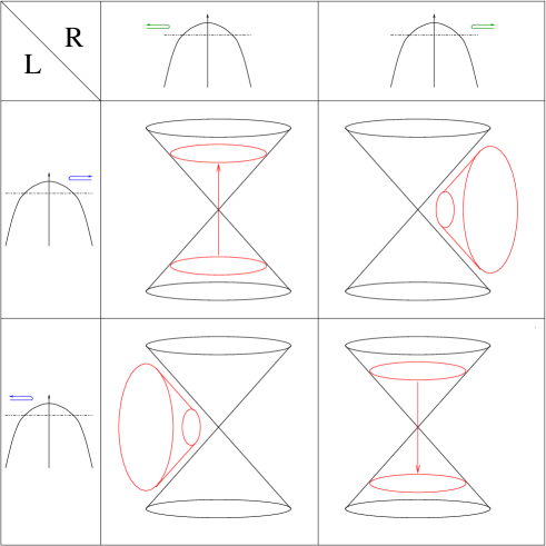
Figure 1: Winding strings on the Lorentzian orbifold exist in two different species: short strings (wrapping the Milne circle) and long strings (stretched from Rindler infinity to a finite radius and folded back onto themselves). The inverted harmonic potentials refer to the symmetric quantization scheme of Sec. (3.4).

In view of the very different nature of these states, we shall refer to them as short and long winding strings, respectively. For non-vanishing $j$, the situation is much the same, except that the extremal radius reached by the string is now

$$r_{0}^{2}=-2X^{+}X^{-}=\frac{1}{4\nu^{2}}(M-\epsilon\tilde{\epsilon}\tilde{M})^{2}$$ (40)

Long strings therefore stay away from the origin of Rindler patch, while short strings wander for a finite interval $[\tau_{0},\tau_{1}]$ into one of the Rindler patches, depending on the sign of $j$: again, in this region they can be viewed as static strings, which extend from the origin of Rindler space to a finite radius, and fold back onto themselves. In contrast to the long strings, they have finite length at every finite cosmological time $T$. The fact that a string world-sheet winding around a compact time direction is better thought of as a static string is quite general.

It is important to note that the induced metric on the long string solution has unusual causality properties: the world-sheet $\sigma$ direction wraps the target-space time-like direction $\eta$, while the world-sheet $\tau$ direction generates a motion in the space-like radial direction $r$. This also takes place during the interval $[\tau_{0},\tau_{1}]$ for short strings with $j\neq 0$, where the induced metric undergoes a signature flip as the string crosses the horizon. Such a behavior is reminiscent to the case of classical trajectories for tachyonic states in flat space, however here it is found for otherwise sensible physical states with $M^{2}>0,\tilde{M}^{2}>0$. More aptly, it is analogous to the case of supertubes or long strings in Gödel Universe[24, 25]).

There seems to be however no reason to exclude these solutions a priori, since they are bona fide solutions of the Polyakov action in the conformal gauge . We will return to this point in Section 3.5.3, where we quantize the strings from the point of view of an observer in the Rindler patches.

Finally, the above classical solutions carry over to Grant space, after modifying the quantization condition on $j$ appropriately. The single-valued coordinates $z^{\pm}$ introduced in (17) are now independent of the $\sigma$ coordinate,

$$Z_{0}^{\pm}(\tau,\sigma)=\pm\frac{1}{2\nu}\alpha_{0}^{\pm}e^{\pm\nu\tau}\mp\frac{1}{2\nu}\tilde{\alpha}_{0}^{\pm}e^{\mp\nu\tau}$$ (41)

so that the string center of motion follows a particular world-line in the Grant geometry, while the string itself wraps the compact coordinate $x$. It is easy to see that the matching conditions imply that, for long strings, the extremal radius $r_{0}$ always lies in the region where the coordinate $x$ is time-like. Short strings on the other hand come from infinite past, cross the chronological horizon $z^{+}z^{-}=0$ and return into the future patch, much as in the original Misner geometry. For appropriate choices of $j$ and $p$, they may cross over into the $r_{0}>1/E$ region.

3.3 From Twisted Closed Strings to Charged Particles

As observed in [14], the closed string zero-mode (29) is strikingly reminiscent of the classical trajectory of a charged particle (or string) in an electric field

$$X^{\pm}(\tau)=x_{0}^{\pm}\pm\frac{a_{0}^{\pm}}{\nu}e^{\pm\nu\tau}$$ (42)

Clearly, the world-line of the charged particle mode $(x_{0}^{\pm},a_{0}^{\pm})$ can be mapped to the motion of a point at fixed $\tau+\sigma$ on the twisted closed string world-sheet, upon identifying

$$x_{0}^{\pm}=\mp\frac{1}{2\nu}\tilde{\alpha}_{0}^{\pm}\ ,\quad a_{0}^{\pm}=\frac{1}{2}\alpha_{0}^{\pm}$$ (43)

Since the closed string zero-mode (29) depends on $\sigma$ only through the boost action, it is thus straightforward to obtain the entire closed string world-sheet by smearing the charged particle trajectories under the boost action. Charged particle trajectories which remain inside the Rindler patches are thus associated to long string configurations, while charged particle trajectories which cross the Rindler horizon are associated to short strings.

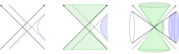
Figure 2: The twisted string world-sheet can be obtained by smearing the charged particle trajectory under the action of the boost. Charged particles crossing the Rindler horizon correspond to short strings (in green), while charged particles escaping to Rindler infinity correspond to long strings (in blue).

This embedding can be used to simplify the first quantization of the twisted closed string. At the quantum level, the closed string zero-modes algebra (34) is also isomorphic to the charged particle algebra under the identification (43). This implies that we can use the same representation in terms of covariant derivatives acting on wave functions of two coordinates $x_{+},x_{-}$ as in the charged particle case,

$$\alpha_{0}^{\pm}=i\nabla_{\mp}=i\partial_{\mp}\pm\frac{\nu}{2}x^{\pm}\ ,\quad\tilde{\alpha}_{0}^{\pm}=i\tilde{\nabla}_{\mp}=i\partial_{\mp}\mp\frac{\nu}{2}x^{\pm}$$ (44)

in such a way that the physical state conditions are simply the Klein-Gordon operators for a particle with charge $\pm\nu$ in a constant electric field,

$$M^{2}=\nabla_{+}\nabla_{-}+\nabla_{-}\nabla_{+}\ ,\quad\tilde{M}^{2}=\tilde{\nabla}_{+}\tilde{\nabla}_{-}+\tilde{\nabla}_{-}\tilde{\nabla}_{+}$$ (45)

To understand the physical meaning of the $x^{\pm}$ coordinates in the closed string setting, observe that in this representation, the zero-mode (29) reads

$$X^{\pm}_{0}(\sigma,\tau)=e^{\mp\nu\sigma}\left[\frac{1}{2}\cosh(\nu\tau)~{}x^{\pm}\pm\frac{i}{\nu}\sinh(\nu\tau)~{}\partial_{\mp}\right]=\frac{1}{2}x^{\pm}~{}~{}~{}\mbox{at}~{}\tau=\sigma=0$$ (46)

The coordinates $x^{\pm}$ are thus (up to a factor of 2) the (Schrödinger picture) operators corresponding to the location of the closed string at $\sigma=0$. The radial coordinate $r=\sqrt{-2x^{+}x^{-}}$ associated to the coordinate representation (44), should be thought of as the radial position of the closed string in the Rindler wedges at a fixed $\tau$. On the other hand the world-sheet dependence on the angular coordinate (for a given winding number) is fixed in terms of the boost momentum $j$.

The physical state conditions are most usefully imposed in this representation on $\mu^{2}=(M^{2}+\tilde{M}^{2})/2$ and on $j=(M^{2}-\tilde{M}^{2})/(2\nu)$. The wave functions for the radial location of the twisted closed string modes are thus the same as the radial part of the quantum wave functions for charged particles in an electric field, with boost momentum $j=i(x^{+}\partial_{+}-x^{-}\partial_{-})$ given by the quantized value (36).

We can therefore make use of the discussion of charged particle wave functions in Rindler coordinates [14, 26], and obtain the wave functions in the right Rindler patch as zero-energy modes of the Schrödinger operator $-\frac{d^{2}}{dy^{2}}+V(y)=0$, with potential

$$V(y)=M^{2}r^{2}-\left(j+\frac{1}{2}\nu r^{2}\right)^{2}=\frac{M^{2}\tilde{M}^{2}}{\nu^{2}}-\left(\frac{M^{2}+\tilde{M}^{2}}{2\nu}-\frac{\nu}{2}r^{2}\right)^{2}$$ (47)

where $r=e^{y}$. Assuming that the state is non-tachyonic, i.e. $M^{2}>0$ and $\tilde{M}^{2}>0$, the potential includes a classically forbidden region, with turning points given by (40). Depending on the sign of $j$, this corresponds to the tunneling of a long string coming from Rindler infinity into a short string going forward ($j<0$) or backward ($j>0$) in time. The wave functions ${\cal U}_{in,R}^{j}$ and ${\cal V}_{in,R}^{j}$ introduced in [26, 14] can now be interpreted as operators creating a long string stretching from infinity, resp. a short string stretching into the horizon.

It is perhaps enlightening to describe the tunneling process semi-classically. As usual in ordinary quantum mechanics, tunneling can be described by continuing the proper time $\tau$ to the imaginary axis, i.e. solving the Schrödinger equation (47) in the flipped potential $-V(y)$. One thus obtains an Euclidean world-sheet stretching between the long and short string world-sheet, i.e. between two hyperbolas centered at the origin in the Rindler wedges. Alternatively, one may keep using a Lorentzian world-sheet but analytically continue the target space, i.e. rotate $\nu\to i\nu$ as well as change the reality conditions on $X^{\pm}$ to $(X^{\pm})^{*}=\pm X^{\mp}$. This maps the Lorentzian orbifold in the Rindler regions to the Euclidean rotation orbifold, $Z\equiv e^{i\beta}Z$. The tunneling trajectories now describe closed strings trapped at the tip of the conical singularity and oscillating between an inner and outer radius $r^{\pm}$. It would be tempting to use this analytic continuation at $X^{0}<0$ to define a Hartle-Hawking type of vacuum in the Rindler regions, however such a prescription does not seem to be consistent with the orbifold identification. We shall return to this issue in Section 4, and argue that the correct picture to describe winding string production is the “EM” one: Euclidean world-sheet and Lorentzian target space.

For a given choice of vacuum, we can now obtain the pair production rate by simply evaluating the Bogolubov coefficients, i.e. the overlap of the corresponding wave functions. The transmission coefficients in the Rindler and Milne regions can be read off from [26, 14],

$$q_{2}=e^{-\pi M^{2}/2\nu}\frac{|\sinh\pi j|}{\cosh\left[\pi\tilde{M}^{2}/2\nu\right]}\ ,\quad q_{4}=e^{-\pi M^{2}/2\nu}\frac{\cosh\left[\pi\tilde{M}^{2}/2\nu\right]}{|\sinh\pi j|}\ ,$$ (48)

respectively. As in the Schwinger effect, tunneling corresponds to induced pair production, and implies that spontaneous pair production takes place as well. From (48), one notices that the production rate in the Milne regions $q_{4}$ is infinite for vanishing boost momentum $j=0$, while the production rate in the Rindler regions vanishes. This can be traced to the fact that the energy of the tunneling process becomes equal to the potential energy at the horizon $y\to\infty$, leading to the production of a non-normalizable state. For $j$ non-zero, and holding the contribution of excited and transverse modes $M^{2},\tilde{M}^{2}$ fixed, the rate $q_{4}$ diverges linearly in $w$ as the winding number grows to infinity. As we shall see in Section 5, this can be viewed as a consequence of the singular geometry, and resolving it leads to a finite production rate at $j=0$ (or $w=\infty$).

Given the wave function in the Rindler patch, there are many ways to analytically continue it across the horizons to other patches, consistently with charge conservation. Among these various choices, those which involve only analytic continuation into the upper half of the complex $x^{+}$ and $x^{-}$ planes play a special rôle: they have support on positive energy states as measured by a static observer in the Minkowski covering space. These global modes are usually known as Unruh modes in the neutral case, and we will keep this name in our case as well. In Figure 3, we have represented two examples of Unruh modes for a charged particle, and their interpretation in terms of winding strings. Just as in the untwisted sector case, Unruh modes should be the positive energy modes implicit in the perturbative string expansion.

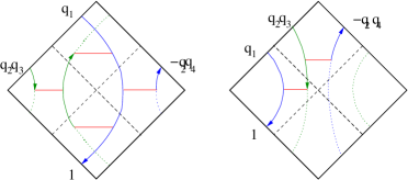
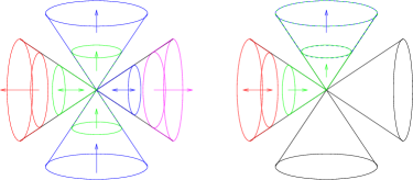
Figure 3: Global Unruh modes for a charged particle in an electric field (left), and their interpretation as closed string wave functions (right). The latter are obtained by smearing the charged particle wave function over the action of continuous boosts.

3.4 Oscillator Representation

We now come to an alternative representation of the closed string zero modes, which treats left and right movers symmetrically. The zero mode algebra (34) consists of two harmonic oscillators. Motivated by the standard treatment of the harmonic oscillator we can represent the zero mode on the space of functions $f(\alpha^{+},\tilde{\alpha}^{-})$, with

$$\alpha^{-}=i\nu\partial_{\alpha^{+}},\ \ \ \tilde{\alpha}^{+}=i\nu\partial_{\tilde{\alpha}^{-}}$$ (49)

The Virasoro constraints then requires that the wave function depends on $\alpha^{+},\tilde{\alpha}^{-}$ as a power,

$$f(\alpha^{+},\tilde{\alpha}^{-})=\left(\epsilon~{}\alpha^{+}\right)^{\frac{M^{2}}{2i\nu}-\frac{1}{2}}\left(\tilde{\epsilon}~{}\tilde{\alpha}^{-}\right)^{\frac{\tilde{M}^{2}}{2i\nu}-\frac{1}{2}}\ ,$$ (50)

up to a normalization factor. The choice of signs $\epsilon,\tilde{\epsilon}$ is correlated with the short and long string branches discussed in Section 3.2. In addition to its simplicity, the interest of this representation stems from the fact that eigenstates (50) can be obtained from the oscillator states $(a^{\dagger})^{n}(\tilde{a}^{\dagger})^{\tilde{n}}$ of the standard (Euclidean) harmonic oscillator by analytically continuing the integers $(n,\bar{n})$ to complex values [27].

The relation of this representation to the real-space $(x^{+},x^{-})$ representation (44) may be obtained by diagonalizing simultaneously $\alpha^{+}$ and $\tilde{\alpha}^{-}$, leading to

$$f(x^{+},x^{-})=\int d\alpha^{+}d\tilde{\alpha}^{-}\Phi^{+}_{\nu,\alpha^{+},\tilde{\alpha}^{-}}(x^{+},x^{-})f(\alpha^{+},\tilde{\alpha}^{-})$$ (51)

where

$$\Phi^{+}_{\nu,\alpha^{+},\tilde{\alpha}^{-}}(x^{+},x^{-})=\exp\left(\frac{i\nu x^{+}x^{-}}{2}-i\alpha^{+}x^{-}-i\tilde{\alpha}^{-}x^{+}+\frac{i}{\nu}\alpha^{+}\tilde{\alpha}^{-}\right)$$ (52)

Alternatively, one may choose to diagonalize $\alpha^{-}$ and $\tilde{\alpha}^{+}$, leading to

$$f(x^{+},x^{-})=\int d\tilde{\alpha}^{+}d\alpha^{-}~{}\Phi^{+}_{\nu,\tilde{\alpha}^{+},\alpha^{-}}(x^{+},x^{-})~{}f(\tilde{\alpha}^{+},\alpha^{-})$$ (53)

where

$$\Phi^{-}_{\nu,\tilde{\alpha}^{+},\alpha^{-}}(x^{+},x^{-})=\exp\left(-\frac{i\nu x^{+}x^{-}}{2}-i\tilde{\alpha}^{+}x^{-}-i\alpha^{-}x^{+}-\frac{i}{\nu}\tilde{\alpha}^{+}\alpha^{-}\right)$$ (54)

On shell wave functions in this representation are related to (50) by Fourier transform, and are now given by

$$f(\tilde{\alpha}^{+},\alpha^{-})=\left(\tilde{\epsilon}~{}\tilde{\alpha}^{+}\right)^{-\frac{\tilde{M}^{2}}{2i\nu}-\frac{1}{2}}\left(\epsilon~{}\alpha^{-}\right)^{-\frac{M^{2}}{2i\nu}-\frac{1}{2}}$$ (55)

up to normalization. The kernels (52) and (54) can be thought as the analogue, for twisted states, of the off-shell wave functions $e^{-ik^{+}x^{-}-ik^{-}x^{+}}$ in Minkowski space.

Upon substituting in (53) the wave function (50), and integrating over $\alpha^{+}$, $\tilde{\alpha}^{-}$ in one of the four quadrants, one obtains in principle an on-shell wave function – provided the integral is well defined. Defining $\alpha^{+}=\epsilon ue^{v},\tilde{\alpha}^{-}=\tilde{\epsilon}ue^{-v}$ with $u>0$, one can first perform the angular integral, obtaining the same wave functions as in the untwisted case: for a short string moving forward in time ($\epsilon=\tilde{\epsilon}=1$), one obtains

$$f(x^{+},x^{-})=\int_{0}^{\infty}dr\left[\left(\frac{x^{+}}{x^{-}}\right)^{-ij/2}H^{(1)}_{-ij}(2r\sqrt{x^{+}x^{-}})\right]r^{\frac{i(M^{2}+\tilde{M}^{2})}{2\nu}}e^{ir^{2}/\nu}$$ (56)

with the Hankel function $H^{(1)}$ being replaced by $H^{(2)}$ in the time-reversed case. On the other hand, for a long string in the right Rindler patch ($\epsilon=-\tilde{\epsilon}=-1$), the wave function appearing after the $v$ integration corresponds to the wave function for a tachyonic untwisted state. Again, we stress that long strings are nevertheless non-tachyonic physical states with $M^{2},\tilde{M}^{2}>0$.

It is also instructive to carry out the integration in reversed order. The radial integration leads to a parabolic cylinder function, which in the limit of large $|v|$ is dominated by the saddle point value,

$$f(x^{+},x^{-})\propto\int_{-\infty}^{\infty}dv\left[\left(\tilde{\epsilon}x^{-}e^{v}+\epsilon x^{+}e^{-v}\right)\right]^{\frac{M^{2}+\tilde{M}^{2}}{2i\nu}}\exp\left[-\frac{i\nu\epsilon\tilde{\epsilon}}{4}\left((x^{+})^{2}e^{-2v}+(x^{-})^{2}e^{2v}\right)-ijv\right]$$ (57)

Comparing to the untwisted case (7), we see that this expression is well defined as an integral over the real $v$ axis only when the spin $s=\Im(j)<2$, which is a (minor) improvement over the untwisted case. For higher values one should deform the $v$ integration contour in the complex plane as in (7). Equivalently, one should continue $x^{\pm}\to x^{\pm}-i~{}\mbox{sgn}(\epsilon\tilde{\epsilon}x^{\pm})~{}0^{+}$: the required analytic continuation is thus different for long and short strings. We shall return to the analyticity properties of these wave functions when we discuss second quantization in Section 3.5.1 below.

3.5 Second Quantization

Having described the first quantization of the twisted sector zero-modes $\alpha_{0}^{\pm},\tilde{\alpha}_{0}^{\pm}$ on the closed string world-sheet, we now come to the issue of the second quantization of the resulting continuum of physical states. As we are dealing with a time-dependent geometry, we expect a variety of vacua, depending on the kind of observer:

• String perturbation theory presumably picks the “Minkowski” vacuum, defined with respect to the $x^{0}$ time variable on the covering space. While creation and annihilation operators are usually discriminated by their analyticity properties in the complex $x^{0}$ plane, we will see that long strings have no such analyticity property (in line with their other tachyon-like features) and an ad hoc prescription must be devised for them: we propose that they be distinguished by the sign of their boost momentum $j$ , which generates time evolution in the Rindler patches. We will show in Section 4.2 that the string vacuum amplitude has no imaginary part, which implies that there should be no overall pair production in this vacuum.

• On the other hand, one may be interested in the vacuum defined by an accelerated observer in the Rindler patch, i.e. an observer sitting at a fixed radius in one of the Rindler patches. This choice is particularly appealing since the geometry in the Rindler patch is time-independent, and states can be quantized unambiguously according to the sign of their energy (after deciding on an arrow of time in each of the Rindler regions). In addition, the line $x^{0}=0$ is the most natural Cauchy surface in the geometry, and one may describe the global quantum state as a state in the tensor product of the left and right Rindler patches. This would allow a description of the cosmological evolution in the Milne patch by standard time-independent techniques, adapted to the existence of CTCs. As we shall see, one problem with this vacuum is that short strings have an unbounded negative energy spectrum, which, at least in the absence of CTCs, would lead to an instability.

• As in the untwisted case, one may choose to define a “conformal” vacuum in terms of the behavior as $T\to 0$ in the Milne patch. This procedure will however miss the long string states, which live in the Rindler patches only and never approach the horizon. We will not discuss these vacua any further here.

• More radically, one may choose to quantize with respect to the radial coordinate $r$ in the Rindler patches. This procedure would be natural from an holographic point of view, where one would impose boundary conditions at Rindler infinity, and let them evolve into the bulk. This is already suggested by the long strings, which propagate radially rather than forward in time under the world-sheet time evolution. However, this procedure would miss the short string states, which do not propagate to Rindler infinity.

Finally, one may push the analogy to the charged particle to the level of second quantization, and devise a closed string vacuum modeled on the $in$ and $out$ vacua for charged particles in an electric field. Since treating the left and right moving zero-modes $\alpha_{0}^{\pm}$ and $\tilde{\alpha}_{0}^{\pm}$ symmetrically and independently does not lead to an unambiguous prescription for the long strings, one may instead choose to identify one side with the center of motion coordinate $x_{0}^{\pm}$ and the other with the velocity $a_{0}^{\pm}$ of the charged particle (as in Section 3.3), and inherit a well defined prescription for $in$ and $out$ vacua. However, making the opposite choice would lead to different vacua, so the physical interpretation of these vacua is unclear. This is so partially due to their inherently stringy nature, as they treat the left and right movers asymmetrically.

Irrespective of the choice of vacua, Bogolubov coefficients, hence the global pair production rate, are given by the overlap of the the zero-mode wave functions, or equivalently by the two-point function of twisted fields at tree-level, after a basis for in and out states is chosen (see e.g. [28] for a related conclusion).

We now supply some details on the vacua outlined above.

3.5.1 Minkowski Vacuum

In the untwisted sector one divides operators uniquely into creation and annihilation by requiring that wave packets built out of creation operators are analytic in the lower half plane of the complex time coordinate. In Minkowski space, this is equivalent to saying that the wave functions $e^{-iEx^{0}}$ corresponding to creation operators have positive energy, $E>0$. We will try and implement this definition for the twisted sector.

For this, we return to the oscillator representation (50), and analyze the analyticity properties of the wave function in real space $f(x^{+},x^{-})$. For the short string $(\epsilon,{\tilde{\epsilon}})=(1,1)$ case, the kernel picks up a converging factor $\exp(-(\alpha^{+}+\alpha^{-})0^{+})$ upon continuing $x^{\pm}\to x^{\pm}-i0^{+}$: the resulting mode is thus analytic and bounded in the lower $x^{0}$ half plane, hence, from the discussion in Section 2.2, should correspond to a creation operator in the (Minkowski) covering space vacuum. Similarly, for $(\epsilon,{\tilde{\epsilon}})=(-1,-1)$ the mode is analytic and bounded in the upper $x^{0}$ half plane, hence corresponds to an annihilation operator.

On the other hand, for the long string $\epsilon\tilde{\epsilon}=-1$ case, it is easy to see that the kernel $\Phi$ is analytic and bounded neither in the upper nor in the lower half plane, hence cannot be assigned any definite quantization rule on this basis alone. However, recall that the classical long string solutions are localized within one of the Rindler wedges depending on the signs of $\epsilon$ and ${\tilde{\epsilon}}$: for $(\epsilon,{\tilde{\epsilon}})=(1,-1)$ they were localized in the region $x^{+}>0,\ x^{-}<0$. This fact carries over to the quantum wave function in a standard way - the function will decay rapidly at infinity unless a stationary phase exists for $(\alpha_{0}^{+},\tilde{\alpha}_{0}^{-})$, which for $(\epsilon,{\tilde{\epsilon}})=(1,-1)$ indeed happens only for $x^{+}>0,\ x^{-}<0$. Moreover, the Lorentz boost operator $j$ evolves forward in the right Rindler region $R$, and backward in the left Rindler region $L$, with respect to the time orientation on the covering space. It is thus natural to split the long string states into creation and annihilation operators according to the sign of the product $\mbox{sgn}(j)\epsilon$: in this way, creation operators will indeed evolve forward in Minkowski time.

In this prescription $j=0$ states should be thought of as “zero modes” of the configuration. Note that $j$ is quantized, hence these zero modes are not part of a continuum. Rather they are like 0+1 dimensional quantum mechanical modes (for example String theory compactified in all directions spatial will have isolated vertex operators with zero momentum in all directions, and zero energy for massless fields). The situation here is particularly pathological from this point of view - these modes exist for any value of $M$, as long as ${\tilde{M}}^{2}=M^{2}$ and hence can happen at for any transverse momentum and for every oscillator number.

3.5.2 Charged Particle Vacua

In the oscillator representation (49), the wave function factorizes into a product of wave functions for the left and right movers, each of which corresponding to eigenmodes of an inverted harmonic oscillator. As discussed in [14], the same situation is encountered when quantizing a particle in an electric field in static coordinates: states bouncing on the right of the potential barrier are interpreted as electrons propagating forward in time, while states bouncing on the left side of the potential are positrons propagating backward in time – tunneling under the barrier being simply Schwinger induced pair production. In addition, the charged particle has spectator translational zero-modes $x^{\pm}_{0}$. The closed strings modes $\alpha^{\pm}_{0}$ and $\tilde{\alpha}^{\mp}_{0}$ can thus be interpreted as a pair of charged particles with opposite charge, upon disregarding their translational zero-modes.

On the basis of this analogy, one may therefore quantize the closed string modes according to their charged particle interpretation. Short strings with $(\epsilon,\tilde{\epsilon})=(1,1)$ correspond to the tensor product of an electron and a positron, both of them propagating forward in time: according to our rule, it is thus a creation operator. Similarly, short strings with $(\epsilon,\tilde{\epsilon})=(-1,-1)$ correspond to the tensor product of a positron and an electron, both of them propagating backward in time, hence are annihilation operators. On the other hand, long strings with $(\epsilon,\tilde{\epsilon})=\pm(1,-1)$ correspond to the tensor product of two electrons (or positrons), one of which propagating forward in time while the other one propagates backward. This rule therefore does not determine the vacuum for long strings.

However, motivated by the discussion in Section 3.3, we may break the symmetry between the left and right movers, and choose a particular identification of the closed string modes $(\alpha_{0}^{\pm},\tilde{\alpha}_{0}^{\pm})$ with the charged particle’s $(a_{0}^{\pm},x_{0}^{\pm})$, say relation (43). As we discussed in Section 3.3, the physical states are now eigenmodes of the Schrödinger equation (47) describing charged particles in an electric field from the point of view of an accelerated observer. As explained in [26, 14], there is now an unambiguous way to quantize the system in each of the Rindler patches, depending on the sign of $\epsilon$: in this prescription, short strings propagating forward in time and long strings living in the right Rindler patch are creation operators, while short strings propagating backward in time and long strings living in the left Rindler patch are annihilation operators. In order to completely specify the vacuum, one should specify the basis of wave functions according to their behavior at infinity or on the light-cone, and apply the above rule to the dominant part of the wave function. As explained above, there is an ambiguity in this prescription which of the left or right moving zero-modes $\alpha^{\pm}_{0}$ and $\tilde{\alpha}^{\pm}_{0}$ is identified with the charged particle’s $x_{0}^{\pm}$. We see that the two possible choices lead to two different prescriptions for the long string modes.

3.5.3 Quantization in the Rindler Patch

We now discuss the second quantization from the point of view of an observer sitting at a fixed radius $r$ in one of the Rindler patches. As emphasized in Section 3.2, for strings which propagate in the Rindler region (be it long or short strings), the world-sheet time $\tau$ generates a radial motion, while the $\sigma$ direction winds around the compact time coordinate $\eta=w\sigma$. It is thus natural to first quantize the string with respect to $\sigma$ evolution, rather than $\tau$. The energy measured by a Rindler observer, corresponding to translations of time $\eta$, is now given by an integral over the non-compact $\tau$ coordinate,

$$W=-\int_{-\infty}^{\infty}d\tau\left(X^{+}\partial_{\sigma}X^{-}-X^{-}\partial_{\sigma}X^{+}\right)=\int_{-\infty}^{\infty}d\tau R^{2}\partial_{\sigma}\eta$$ (58)

while the mass-shell conditions, $M^{2}=2\alpha_{0}^{+}\alpha_{0}^{-}$ and its tilded counterpart, are unchanged since, at the zero-mode level, the world-sheet energy-momentum tensor is independent of $\sigma$ and $\tau$, and hence leads to the same Virasoro conditions (up to an infinite multiplicative factor) in either quantization scheme.

Notice in particular that the Rindler energy has nothing to do with the boost momentum $j=(M^{2}-\tilde{M}^{2})/(2\nu)$ which was found for the usual $\tau$ evolution, rather it is proportional to the winding number $w$. In particular, in this quantization scheme there appears to be no reason to quantize the boost momentum $j$, but rather $W$ should be quantized in units of $1/\beta$. Nevertheless, if one continues to quantize the oscillators in the same way, the quantization of $j$ will still result from the matching condition.

The Rindler energy (58) diverges, as expected for an infinitely extended open string. Nevertheless, it is easy to compute the Rindler energy density, by unit of radial element,

$$W=\int_{-\infty}^{\infty}w(r)~{}\frac{dr}{d\tau}~{}d\tau$$ (59)

where

$$w(r)=\frac{4\nu^{2}r^{3}\mbox{sgn}(\nu)}{\sqrt{(M^{2}+\tilde{M}^{2}-4\nu^{2}r^{2})^{2}-4M^{2}\tilde{M}^{2}}}$$ (60)

This energy density diverges as $(r-r_{0})^{-1/2}$ at the turning point $r=r_{0}$, but the singularity is integrable. As $r\to\infty$, for long strings at $r\to\infty$, the energy diverges quadratically, as a result of the infinite tensive energy (positive for $w>0$) stored at large radius. For short strings, one should instead integrate over $r\in[0,r_{0}]$, as the string spends only a finite interval $\tau[\tau_{0},\tau_{1}]$ in the Rindler patch. However it is not consistent with energy conservation to truncate to an interval, and indeed energy leaks from the Rindler patch to the Milne patch. Rather, integrating over the full time axis, one finds an infinite large negative value (for $w>0$). In the absence of CTC, this would lead to the conclusion that the Rindler vacuum defined by classifying states according to the sign of $W$ is in fact unstable. It would be interesting to understand whether the compactness of $\eta$ somehow alleviates this instability.

4 One-loop String Vacuum Amplitude

In this Section, we discuss the calculation and interpretation of the one-loop partition function. In particular, we discuss the various divergences and their relation to Euclidean periodic trajectories various decay modes. The issues of particle creation, divergent energy-momentum tensors and back-reaction intimately depend on the choice of vacuum. We will be able to obtain only partial results, with the particular choice of vacuum implicit in the orbifold prescription of string theory.

For orientation purposes, we start by reviewing the case of charged open strings in an electric field, first discussed in [31]. We emphasize some subtleties in the analytic continuation, both on the world-sheet and in target space, and argue that the one-loop amplitude should be properly viewed as a path integral over Euclidean world-sheet and Lorentzian target space. We then adapt the semi-classical methods developed in [32] for the ordinary, field-theoretic, Schwinger effect to the string theory setting, recovering the standard pair creation rate of charged open strings from an analysis of the periodic trajectories in imaginary time.

We then return to the subject of Misner space, and analyze the one-loop vacuum amplitude, both in the untwisted and twisted sectors. In the former case, while local divergences of the energy-momentum found at the field theory level in Section 2.4 disappear in string theory upon integration over space-time, we find new divergences (appearing for the open string as well) arising from the sum over Regge trajectories required in string theory. This genuine stringy feature should play a rôle quite generally in string theory near cosmological singularities.

We then study the twisted sectors, and analyze the imaginary periodic orbits in analogy with the open string case. Upon regulating the singularities of the one-loop amplitude appropriately, we find that the vacuum amplitude remains real, despite the fact that the Euclidean action has instabilities towards condensation of large winding strings. We thus conclude that localized particle creation, and therefore back-reaction on the geometry, does take place in generic vacua.

4.1 Charged Open Strings in an Electric Field

Let us start by recalling the Schwinger computation of pair production of charged particles in an electric field, at the field-theory level.

4.1.1 Analytic Continuation and Production Rate

Using the standard Schwinger proper-time representation

$$\log\frac{a}{b}=\int_{0}^{\infty}\frac{d\rho}{\rho}\left(e^{i\rho(b+i\epsilon)}-e^{i\rho(a+i\epsilon)}\right)$$ (61)

the logarithm of the vacuum-to-vacuum amplitude for a charged particle of mass $M$, charge $\nu$ and spin $s$ can be written as the “MM” integral (for Minkowski world-sheet – Minkowski target space)

$${\cal F}=-\frac{1}{2(2\pi)^{D-2}}\int_{0}^{\infty}\frac{d\rho}{\rho^{D/2}}\left[\frac{\nu}{\sinh(\nu\rho)}\chi_{s}(\rho)-\frac{2s+1}{\rho}\right]e^{-i(M^{2}-i\epsilon)\rho}$$ (62)

where $\chi_{s}(\rho)=\sinh[(2s+1)\nu\rho]/{\sinh(\nu\rho)}$ is the character of the $SU(2)$ representation of spin $s$. The second term in the bracket corresponds to the subtraction of the one-loop vacuum amplitude in the absence of an electric field. This integral suffers from the usual ultraviolet divergences at $\rho\to 0$, which give rise to a renormalization of the action of the electromagnetic field. Thanks to the Feynman $i\epsilon$ prescription, the integral converges in the infrared $\rho\to\infty$, however only for spin $|s|<1$. In this case only, one may rotate the integration contour in the upper half plane, and rewrite (62) as an “EM” integral (Euclidean world-sheet, Minkowski target space),

$${\cal F}=-\frac{i^{D/2}}{2(2\pi)^{D-2}}\int_{0}^{\infty}\frac{d\rho}{\rho^{D/2}}\left[\frac{\nu\sin[(2s+1)\nu\rho]}{\sin^{2}(\nu\rho)}-\frac{2s+1}{\rho}\right]e^{-M^{2}\rho}$$ (63)

where the contour runs slightly to the right of the poles at $\nu\rho=k\pi$. Using the standard principal part prescription $[x-i\epsilon]^{-1}=P(1/x)+2\pi i\delta(x)$ , one finds that, just as the original result (62), the dispersive (real) part of ${\cal F}$ is given by a finite principal part (except for the ultraviolet logarithmic divergence at $\rho=0$), while the dissipative (imaginary) part of ${\cal F}$, hence the pair production rate, is a sum of residues

$${\cal W}=\Im{\cal F}=\frac{1}{2(2\pi)^{D-1}}(2s+1)\sum_{k=1}^{\infty}(-1)^{F(k+1)}\left(\frac{|\nu|}{k}\right)^{D/2}\exp\left(-\pi k\frac{M^{2}}{|\nu|}\right)$$ (64)

Note that the principal part prescription does not strictly follow from Feynman’s $i\epsilon$ prescription, however it is necessary in order to recover the manifestly finite result (62). Note also that in field theory, rotating the Schwinger parameter $\rho\to i\rho$ is essentially equivalent to rotating the electric field to a magnetic field.

For spins $|s|>1$ however, the MM integral (62) is ill-defined in the infrared. On the other hand, the EM integral (63) is perfectly well defined, leading to a consistent production rate (64), sum of contributions of the various helicity states, and a finite dispersive part. Our attitude is therefore to take the EM integral (63) as the fundamental observable, and obtain (62) by analytic continuation $\rho\to e^{i\theta}\rho$, with $\theta$ ranging from $0$ to $\pi/2$. For spin $|s|>1$, it is easy to see that the rotation ceases to be valid at $\tan\theta=M^{2}/(2s-1)\nu$, where the contribution at infinity does not vanish anymore. This divergence is simply the reflection of the Nielssen-Olesen tachyonic instability of a massive charged particle of spin $s\geq 1$ in a magnetic field [33], which would have been encountered if one were rotating the electric field instead. Just as the Schwinger instability relaxes the electric field, the Nielssen-Olesen instability relaxes the magnetic field to zero [34].

4.1.2 Periodic Trajectories and Schwinger Production Rate

We now wish to rederive the stringy Schwinger production rate from a different point of view, which emphasizes the semi-classical interpretation of the process as an instanton, as explained in [32]. For simplicity, we recall the argument in the case of a charged scalar particle in an electric field. As in the Schwinger approach, we start with the first-quantized representation of the free-energy (i.e. the logarithm of the vacuum-to-vacuum transition amplitude),

$$\mathcal{F}=-\int_{0}^{\infty}\frac{d\rho}{\rho}\int[DX(\tau)]~{}e^{-S[X]}$$ (65)

where $S$ is the action for a particle of charge $\nu$ in an electric field in imaginary proper time,

$$S[X]=2\pi M^{2}\rho+\int_{0}^{2\pi\rho}\left[\partial_{\tau}X^{+}\partial_{\tau}X^{-}-\frac{i\nu}{2}\left(X^{+}\partial_{\tau}X^{-}-X^{-}\partial_{\tau}X^{+}\right)\right]d\tau$$ (66)

The path integral is restricted to configurations $X(\tau)$ periodic in imaginary time $\tau$ with period $2\pi\rho$ .

Schwinger’s computation consists in evaluating the path integral over $X(\tau)$ first, obtaining $\mathcal{F}(\rho)$, and then integrate over the proper time $\rho$ to obtain $\mathcal{F}=-\int_{0}^{\infty}\frac{d\rho}{\rho}\mathcal{F}(\rho)$. By the optical theorem, the total decay rate of the vacuum is given by the imaginary part of the free energy. Since the world-line action is real, an imaginary part can only arise from singularities in $\mathcal{F}(\rho)$. However, not all such singularities of $\mathcal{F}(\rho)$ are related to decay processes, for example we will see that singularities in $\mathcal{F}(\rho)$ may also arise from the rapid growth of the density of states, as is the case for the stringy Hagedorn behavior. Therefore, to avoid confusion, we will relate directly periodic classical solutions to decay rates, bypassing whenever possible a discussion of $\mathcal{F}(\rho)$ and its singularities.

Instead, as proposed in [32], one may first carry out the integration over $\rho$, which is of Bessel type after rescaling $\tau\to\rho\tau$. In the saddle point (large $M$) approximation, the integral is peaked around

$$\rho=\frac{1}{M}\sqrt{\int_{0}^{2\pi}d\tau\left(\partial_{\tau}X^{+}\partial_{\tau}X^{-}\right)}$$ (67)

and yields the saddle point action,

$$S=2M\sqrt{\int_{0}^{2\pi}d\tau\left(\partial_{\tau}X^{+}\partial_{\tau}X^{-}\right)}-\frac{i\nu}{2}\int_{0}^{2\pi}d\tau\left(X^{+}\partial_{\tau}X^{-}-X^{-}\partial_{\tau}X^{+}\right)$$ (68)

The path integral is now over periodic configurations in imaginary time with period 1, and can be evaluated semi-classically by expanding around the classical solutions. Despite the apparent non-linearities in (68), classical solutions are still the usual charged particle trajectories, up to a rescaling of imaginary time $\tau\to\rho\tau$,

$$X^{\pm}_{0}(\tau)=x_{0}^{\pm}\pm\frac{{a_{0}^{\pm}}}{\nu}e^{\pm ik\tau}$$ (69)

where the integer $k$ indicates the number of revolutions during the period $2\pi$. The radius of the circle $R^{2}:=2a^{+}a^{-}$ is fixed by the equations of motion resulting from (68) to the on-shell value $R=M$, while the classical action and period are given by

$$S_{k}=\pi kM^{2}/\nu\ ,\quad\rho_{k}=k/\nu$$ (70)

Notice that $\rho_{k}$ is precisely the value of the Schwinger parameter where the one-loop amplitude (64) becomes singular.

In order to evaluate the path integral, one must now compute the determinant of fluctuations around (69). The complete analysis was carried out in [32], where it was found that fluctuations of radius $R$ of the trajectory around the saddle value $R=M$ corresponds to a negative eigenvalue for the action, while other deformations of the trajectory have a positive eigenvalue. In addition, the zero-mode $x_{0}^{\pm}$ of course has zero action and leads to a factor of volume, as appropriate for the total vacuum-to-vacuum transition amplitude. For our purposes, it will be sufficient to concentrate on the radial mode $R$. Evaluating the action (68) (before any rescaling of time) on the off-shell configuration (69), we obtain

$$S[X_{0}]=\frac{\pi k^{2}}{\nu^{2}\rho}\left(1-\frac{\nu\rho}{k}\right)R^{2}+\pi M^{2}\rho$$ (71)

Clearly, when $\rho=k/\nu$ the Gaussian integral over $R^{2}$ diverges, which is the origin of the divergence in (64). However, one may integrate over $\rho$ first, and replace it by its saddle point value $\rho=|k|R/(\nu M)$, obtaining

$$S=\frac{k\pi}{\nu}R(2M-R)$$ (72)

This action indeed has a maximum at $R=M$, leading to an imaginary part for the transition amplitude. The sum over the Euclidean solutions (69) for all $k$, including the one loop determinant, generates the classic Schwinger result for the vacuum decay rate (64) [32].

This semi-classical derivation of the spontaneous production rate is complementary to the semi-classical derivation of induced pair production outlined in Section 3.3. Both processes involve a propagation in imaginary proper time: in the case of induced pair production, the Lorentzian trajectory is continued to Euclidean time at the turning point, evolved through the potential barrier, and continued back to Lorentzian on the other side. In the case of spontaneous pair production, an Euclidean periodic trajectory is cut at mid-period and used as an initial electron-positron state which undergoes subsequent Lorentzian evolution (much as in the Hartle-Hawking prescription for quantum gravity). Since the zero modes $x^{\pm}_{0}$ are arbitrary, the pair production is spatially homogeneous. As we shall see, these two semi-classical pictures carry over to the closed string case, with appropriate adjustments.

4.1.3 Charged Open Strings in an Electric Field

We now briefly proceed to the case of open strings stretched between two D-branes carrying different uniform electric fields $e_{0},e_{1}$ [31, 30]. Such open strings carry an overall charge under the electric field $e_{0}-e_{1}$, hence behave much like charged particles, except for additional polarization effects. In field theory, a standard assumption is that the Schwinger proper time can be rotated from Minkowski to Euclidean without difficulties. We will see that the excited string modes invalidate this lore in string theory.

Starting with the semi-classical approach outlined above, we look for periodic classical trajectories in imaginary world-sheet time. A complete set of classical solutions with those boundary conditions is given by

$$X^{\pm}_{n}(\sigma,\tau)=e^{(n\pm i\nu)\tau}\cos\left[(n\pm i\nu)\sigma\right]$$ (73)

where $\pi\nu=\arctan(\pi e_{0})+\arctan(\pi e_{1})$ [31]. Unless $n=0$, none of these solutions is periodic in Euclidean time. The mode $n=0$ corresponds to the same classical solution (69) for the open string center of motion, therefore the partition function has only the previous set of saddle points. The contribution of the stringy modes to the one loop determinant around each of them can be extracted from the computation by Bachas and Porrati of the one-loop vacuum amplitude, e.g. for the bosonic open string

$$A_{bos}=\frac{i\pi V_{26}(e_{0}+e_{1})}{2}\int_{0}^{\infty}\frac{d\rho}{(4\pi^{2}\rho)^{13}}\frac{e^{-\pi\nu^{2}\rho/2}}{\eta^{21}(i\rho/2)~{}\theta_{1}(\rho\nu/2;i\rho/2)}$$ (74)

where $\theta_{1}$ is the Jacobi theta function,

$$\theta_{1}(v;\rho)=2q^{1/8}\sin\pi v\prod_{n=1}^{\infty}(1-e^{2\pi iv}q^{n})(1-q^{n})(1-e^{-2\pi iv}q^{n})\ ,\quad q=e^{2\pi i\rho}$$ (75)

As in the field-theoretical EM integral above, the poles on the real $\tau$ axis at $\rho=2m/\nu$ contribute to the imaginary part, yielding a sum of the Schwinger pair creation rates (64) over excited states of the open string spectrum (with a mass shift $M^{2}\to M^{2}+\nu^{2}$, in the bosonic string case only). This is the result found in [31].

On the other hand, the partition function has additional poles in the complex $\rho$ plane, at $\rho\nu/2=m+n~{}i\rho/2$. If we were to adopt the prescription of starting from a Minkowskian world-sheet and then rotating $\rho\to i\rho$, these poles would give an extra contribution to the creation rate, equal to

$$\sum_{m,n}e^{-i\pi\nu^{2}\rho/2}\eta^{-24}\left[\frac{m}{n+i\nu}\right]$$ (76)

This prescription would however be in disagreement with the semi-classical reasoning outlined above. We conclude that the Schwinger production rate should not include the contributions of the poles away from the imaginary proper time axis. Thus, computing the imaginary part using the imaginary and the real Schwinger proper time contours gives different results. The two are not equivalent and the additional string poles, associated with excited strings modes, invalidate the standard field theory procedure of analytically continuing from one to the other.

As in the charged particle case, it is possible to understand the origin of the poles at the level of the path integral: For $\rho\nu/2=m+n~{}i\rho/2$, the action corresponding to the excited mode (73) vanishes, and the integral over $a_{n}^{\pm}$ diverges. It is also possible to regard these poles as a consequence of the existence of Regge trajectories in the string spectrum. Indeed, starting with the Schwinger result (64) for fields with arbitrary spin $S$, we see that the sum over an infinite set of states with $M^{2}=M_{0}^{2}+nS$, $S=0\dots\infty$ gives rise to poles in the complex $\rho$ plane at $\rho\nu/2=k+ni\rho/2$. These are precisely the extra poles of the partition function, arising from the Jacobi theta function in the denominator of (74). A similar effect will be shown to occur shortly in the closed string case. However, for the calculation of the pair production rate, these divergences are irrelevant. Indeed the production rate for each particle species depends on the spin through an overall multiplicity factor of $2s+1$, hence remains finite.

To summarize, the lesson is that the decay rate can be read off from the one-loop vacuum amplitude with an Euclidean world-sheet, and a target space signature fixed by the existence of periodic orbits. Poles away from the imaginary world-sheet time axis do not contribute to the pair creation rate, and can be viewed as a consequence of the existence of states with arbitrarily high spin in the spectrum.

4.2 Closed String Theory Vacuum Amplitude

After this detour via open strings in an electric fields, we now return to closed strings in Misner space, and analyze the one-loop vacuum amplitude, computed by path integral and Hamiltonian methods in [7, 10]. The one-loop vacuum amplitude can be written as an “EM” (Euclidean world-sheet, Minkowskian target space) integral on the fundamental domain of the moduli space of the torus,

$$A_{bos}=\int_{{\cal F}}\sum_{l,w=-\infty}^{\infty}\frac{d\rho_{1}d\rho_{2}}{(2\pi^{2}\rho_{2})^{13}}\frac{e^{-2\pi\beta^{2}w^{2}\rho_{2}-\frac{R^{2}}{4\pi\rho_{2}}|l+w\rho|^{2}}}{\left|\eta^{21}(\rho)~{}\theta_{1}\left[i\beta(l+w\rho);\rho\right]\right|^{2}}$$ (77)

where $\rho=\rho_{1}+i\rho_{2}$, and $\theta_{1}$ and $\eta$ are the Jacobi and Dedekind functions,

$$\theta_{1}(v;\rho) = 2q^{1/8}\sin\pi v\prod_{n=1}^{\infty}(1-e^{2\pi iv}q^{n})(1-q^{n})(1-e^{-2\pi iv}q^{n})$$ (78)

$$\eta(\rho) = q^{1/24}\prod_{n=1}^{\infty}(1-q^{n})\ ,\qquad q=e^{2\pi i\rho}$$ (79)

Expanding the inverse of the Jacobi function in powers of $q$, one easily recovers the spectrum of the world-sheet conformal field theory. In particular, as explained in [14], the zero-mode contribution $|\sinh(\beta(l+w\rho)]|^{2}$ can be interpreted either as the contribution of the (left-moving and right-moving) discrete spectrum of the harmonic oscillator in Euclidean time, or as the contribution of the continuous real spectrum of the inverted harmonic oscillator in Lorentzian time.

In this Section, we analyze the target space interpretation of the one-loop amplitude (77), with particular attention to the singularities of the integrand in the moduli space of the torus, at

$$\rho=\frac{k-i\beta l}{n+i\beta w}$$ (80)

where the integer $n$ labels which factor in the product formula of the Jacobi theta function vanishes, and the integer $k$ parametrizes the poles. In contrast to the open string case, these poles occur simultaneously on the holomorphic and anti-holomorphic side, and therefore are not expected to yield an imaginary part, rather, they give rise to logarithmic divergences. Such singularities are very reminiscent of the long string poles appearing in Euclidean AdS₃ [37], and, as we shall see, can also be related to infrared problems.

4.2.1 Untwisted sector

We start with the untwisted sector $w=0$. Expanding in powers of $q$ the inverse of the Dedekind function and the $n\neq 0$ terms of the Jacobi functions, it is apparent that the string theory vacuum amplitude can be viewed as the field theory result (28) summed over the spectrum of (single particle) excited states, satisfying the matching condition enforced by the integration over $\rho_{1}$. As usual, field-theoretical UV divergences at $\rho\to 0$ are cut-off by restricting the integral to the fundamental domain $F$ of the upper half plane. By the standard unfolding trick, one may unfold the integration domain to the strip $[0,1]+i\Real^{+}$ upon restricting the sum to $w=0$.

In contrast to the field theory result, where the integrated free energy is finite for each particle separately, the free energy here has poles in the domain of integration, at

$$\rho=\frac{k-i\beta l}{n}$$ (81)

Those poles arise only after summing over infinitely many string theory states. Indeed, each pole originates from the $(1-e^{\pm 2\pi iv}q^{n})$ factor in (78), hence re-sums the contributions of a complete Regge trajectory of fields with mass $M^{2}=M_{0}^{2}+\alpha^{\prime}p$ and spin $s=p$ ($p\in\mathbb{N}$). In other words, the usual exponential suppression of the partition function by the increasing masses along the Regge trajectory is overcome here by the spin dependence of that partition function. Regge trajectories are a universal feature of perturbative string theory, and we believe that this distinctive stringy effect should manifest itself generically in the presence of space-like singularities. From this point of view, the poles (80) with $w=0$ are related to ultraviolet divergences due to higher spin effects.

Finally, notice that the dependence on the zero-modes $(x^{+},x^{-})$ could be reinstated in the string one-loop amplitude by writing the zero-mode part of the Jacobi function $\sinh^{2}\pi\beta l$ as a Gaussian integral similar to (27). This suggests that the one-loop energy momentum, probed by on-shell vertex operators, will again diverge on the chronology horizon [27]. While this divergence may be somewhat alleviated in the superstring case, we still expect divergences as supersymmetry is explicitly broken by the cosmological background.

4.2.2 Twisted sectors

Let us now turn to the twisted sectors, with $w\neq 0$. The target space interpretation of the one-loop amplitude (77) can be understood by adapting the computation of the charged particle path integral, outlined in Section 4.1.2, to the closed string case. Following the general lesson from section 4.1, we take the target space to be Lorentzian ($X^{\pm}$ real), but rotate the worldsheet time to the imaginary axis. The closed string path integral is given by

$$\mathcal{F}=\int_{F}\frac{d\rho_{1}d\rho_{2}}{\rho_{2}}\sum_{l,w=0}^{\infty}\int[DX]e^{-S_{l,w}}$$ (82)

with action (for $\alpha^{\prime}=1$)

$$S=\frac{1}{2}\int_{0}^{2\pi\rho_{2}}d\tau\int_{0}^{2\pi}d\sigma\left(\partial_{\tau}X^{+}\partial_{\tau}X^{-}+\partial_{\sigma}X^{+}\partial_{\sigma}X^{-}\right)$$ (83)

The path integral is restricted to periodic configurations on the torus of modulus $\rho=\rho_{1}+i\rho_{2}$,

$$X^{\pm}(\sigma+2\pi,\tau)=e^{\pm 2\pi\beta w}X^{\pm}(\sigma,\tau)$$

$$X^{\pm}(\sigma+2\pi\rho_{1},\tau+2\pi\rho_{2})=e^{\mp 2\pi\beta l}X^{\pm}(\sigma,\tau)$$ (84)

where $(-l,w)$ denote the orbifold twists in the $\sigma$ and $\tau$ directions. Interpreting the path integral as the sum of single particle free energies, the integration over $\rho_{1}$ enforces level matching, while $\rho_{2}$ is interpreted as the Schwinger parameter appearing in the previous discussion, with a UV cut-off enforced by the restriction to the fundamental domain $F$

For simplicity, we now restrict the path integral to quasi-zero-mode configurations (which become solutions only when $\rho$ coincides with ones of the poles),

$$X^{\pm}=\pm\frac{1}{2\nu}\alpha^{\pm}e^{\mp(\nu\sigma-iA\tau)}\mp\frac{1}{2\nu}\tilde{\alpha}^{\pm}e^{\mp(\nu\sigma+i\tilde{A}\tau)}$$ (85)

where $\nu=-\beta w$ and

$$A=\frac{k}{\rho_{2}}-i\beta\frac{l+\rho_{1}w}{\rho_{2}}\ ,\quad\tilde{A}=\frac{\tilde{k}}{\rho_{2}}+i\beta\frac{l+\rho_{1}w}{\rho_{2}}$$ (86)

and $k,\tilde{k}$ are a pair of integers labelling the periodic trajectory, for fixed twists $(l,w)$. In order to satisfy the reality condition on $X^{\pm}$, one should restrict to configurations with

$$k=\tilde{k}\ ,\qquad\alpha^{\pm}=-(\tilde{\alpha}^{\pm})^{*}$$ (87)

Nevertheless, for the sake of generality we shall not impose these conditions at this stage. Notice then that for $k=-\tilde{k}$, the world-sheet described by (85) becomes degenerate, and half of the modes, say $\tilde{\alpha}^{\pm}$, should be set to zero to avoid redundancy. This case will be excluded in the following discussion.

We now evaluate the Euclidean world-sheet action (83) for such a configuration,

$$S = \frac{\pi}{2\nu^{2}\rho_{2}}\left(\left[k-i(\beta l+\nu\rho_{1})\right]^{2}-\nu^{2}\rho_{2}^{2}\right)~{}\alpha^{+}\alpha^{-}+\frac{\pi}{2\nu^{2}\rho_{2}}\left(\left[\tilde{k}+i(\beta l+\nu\rho_{1})\right]^{2}-\nu^{2}\rho_{2}^{2}-\right)~{}\tilde{\alpha}^{+}\tilde{\alpha}^{-}$$ (88)

$$-2\pi ij\nu\rho_{1}+2\pi\mu^{2}\rho_{2}$$

where the last line, equal to $-i\pi\rho M^{2}+i\pi\tilde{\rho}\tilde{M}^{2}$, summarizes the contributions of excited modes. It is then convenient to use hyperbolic angular coordinates,

$$\alpha^{\pm}=\pm Re^{\pm\eta}/\sqrt{2}\ ,\qquad\tilde{\alpha}^{\pm}=\pm\tilde{R}e^{\pm\tilde{\eta}}/\sqrt{2}$$ (89)

where the reality condition imposes

$$\tilde{\eta}=\eta^{*}\ ,\quad R^{2}=\tilde{R}^{2}$$ (90)

The integration over the overall angle $\eta+\tilde{\eta}$ gives a finite constant $2\pi\beta$ due to the orbifold identification, while the integration over $\eta-\tilde{\eta}$ gives an infinite factor, independent of the moduli.

In addition, there are divergences coming from the integration over $R$ and $\tilde{R}$ whenever either of the two following conditions are satisfied,

$$\nu\rho_{2}=\pm\left[k-i(\beta l+\nu\rho_{1})\right]\qquad\mbox{or}\qquad\nu\rho_{2}=\pm\left[\tilde{k}+i(\beta l+\nu\rho_{1})\right]$$ (91)

(with uncorrelated signs) The two conditions above are then satisfied simultaneously at

$$\rho_{1}=-\frac{\beta l}{\nu}-i\frac{\nu}{2}(k-\tilde{k})\ ,\qquad\rho_{2}=\frac{|k+\tilde{k}|}{2\nu}$$ (92)

which, for $k=\tilde{k}$, are precisely the double poles (80). We can therefore interpret these poles as coming from infrared divergences due to existence of modes with arbitrary size $(R,\tilde{R})$. For $k\neq\tilde{k}$, the double poles are now in the complex $\rho_{1}$ plane, and may contribute for specific choices of integration contours, or second-quantized vacua. In either case, these divergences may be regulated by enforcing a cut off $|\rho-\rho_{0}|>\epsilon$ on the moduli space, or an infrared cut-off on $R$. It would be interesting to understand the deformation of Misner space corresponding to this cut off, analogous to the Liouville wall in $AdS_{3}$ [37].

Rather than integrating over $R,\tilde{R}$ first, which is ill-defined at $(\rho_{1},\rho_{2})$ satisfying (91), we may choose to integrate over the modulus $\rho,\tilde{\rho}$ first. The integral with respect to $\rho_{1}$ is Gaussian, dominated by a saddle point at

$$\rho_{1}=-\frac{\beta l}{\nu}+i\frac{\tilde{k}\tilde{R}^{2}-kR^{2}}{\nu(R^{2}+\tilde{R}^{2})}-2i\frac{j\nu\rho_{2}}{R^{2}+\tilde{R}^{2}}$$ (93)

It is important to note that this saddle point is a local maximum of the Euclidean action, unstable under perturbations of $\rho_{1}$. The resulting Bessel-type action

$$S=\pi\rho_{2}\left[2\mu^{2}-\frac{1}{2}(R^{2}+\tilde{R}^{2})-\frac{j^{2}\nu^{2}}{R^{2}+\tilde{R}^{2}}\right]+\frac{\pi}{2\nu^{2}\rho_{2}}\frac{(k+\tilde{k})^{2}R^{2}\tilde{R}^{2}}{R^{2}+\tilde{R}^{2}}+2\pi j\frac{kR^{2}-\tilde{k}\tilde{R}^{2}}{R^{2}+\tilde{R}^{2}}-2\pi i\beta jl$$ (94)

has again, for $k+\tilde{k}\neq 0$, a (now stable) saddle point in $\rho_{2}$, at

$$\rho_{2}=\frac{R\tilde{R}|k+\tilde{k}|}{\nu\sqrt{(R^{2}+\tilde{R}^{2})(4\mu^{2}-R^{2}-\tilde{R}^{2})-4j^{2}\nu^{2}}}$$ (95)

Integrating over $\rho_{2}$ in the saddle point approximation, we finally obtain the action as a function of the radii $R,\tilde{R}$:

$$S=\frac{|k+\tilde{k}|R\tilde{R}\sqrt{(R^{2}+\tilde{R}^{2})(R^{2}+\tilde{R}^{2}-4\mu^{2})+4j^{2}\nu^{2}}}{\nu(R^{2}+\tilde{R}^{2})}\pm 2\pi j\frac{\tilde{k}\tilde{R}^{2}-kR^{2}}{\nu(R^{2}+\tilde{R}^{2})}\pm 2\pi i\beta jl$$ (96)

where the sign is that of $k+\tilde{k}$. In analogy with the open string action (72), we may now analyze the behavior of this action as a function of $R$ and $\tilde{R}$. Not surprisingly, we find that it admits an extremum at the on-shell values

$$R^{2}=\mu^{2}-j\nu,\qquad\tilde{R}^{2}=\mu^{2}+j\nu\qquad\mbox{with action}\quad S_{k,\tilde{k}}=\frac{\pi M\tilde{M}}{\nu}|k+\tilde{k}|$$ (97)

Notice that these values are consistent with the reality condition (90), since the boost momentum $j$ is imaginary in Euclidean proper time. Evaluating $(\rho_{1},\rho_{2})$ for the values (97), we reproduce (92), which implies that the integral is indeed dominated by the region around the double pole. Under variations of $R$ and $\tilde{R}$ around the on-shell values (97), we find that the Euclidean action varies as

$$\Delta S=\frac{\pi(k+\tilde{k})}{\nu}\left[(\Delta R)^{2}+(\Delta\tilde{R})^{2}\right]=\frac{2\pi(k+\tilde{k})}{\nu}\left[(\Delta R_{1})^{2}-(\Delta R_{2})^{2}\right]$$ (98)

where $R=R_{1}+iR_{2},\tilde{R}=R_{1}-iR_{2}$, due to the reality condition (90). Together with the negative eigenvalue along $\rho_{1}$ and the positive one along $\rho_{2}$, we find that fluctuations in $(\rho_{1},\rho_{2},R,\tilde{R})$ directions around the saddle point have signature $(+,+,-,-)$, hence a positive fluctuation determinant, equal to $M^{2}\tilde{M}^{2}$ up to a positive numerical constant. This implies that the one-loop amplitude in the twisted sectors does not have any imaginary part, in accordance with the naive expectation based on the double pole singularities. It is also in agreement with the answer in the untwisted sectors, where the globally defined $in$ and $out$ vacua where shown to be identical, despite the occurence of pair production at intermediate times.

Nevertheless, the instability of the Euclidean action under fluctuations of $\rho_{1}$ and $\rho_{2}$ indicates that spontaneous pair production takes place, by condensation of the two unstable modes. Thus, we find that winding string production takes place in Misner space, at least for vacua such that the integration contours picks up contributions from these states. This is consistent with our discussion of the first quantized wave functions, where tunneling in the Rindler regions implies induced pair production of short and long strings. The periodic trajectories (85) describe the propagation across the potential barrier in imaginary proper time, and correspond to Euclidean world-sheet interpolating between the string Lorentzian world-sheets.

5 The Effects of Winding Strings

Our analysis so far has concentrated on the specific case of the Lorentzian orbifold, for which we have shown that winding strings were produced in generic vacua by a tunneling process, analogous to Schwinger pair production of charged particles in an electric field. The all-important question is to determine whether the back-reaction resulting from the production of these states is sufficient, in specific cases, to resolve the cosmological singularity.

As a first step on this direction we investigate the effects of winding string in a class of cosmological backgrounds with a single compact direction, which includes the Misner space. In Section 5.1, we study this problem at a classical level, assuming that a constant number of strings winding along the compact direction have condensed. We find that indeed, for low transverse dimensionality and certain initial conditions, the compact direction may experience a bounce, rather analogous to the usual BKL behavior in inhomogeneous spaces [38].

In Section 5.2, we assume that the back-reaction is described by a mean field deformed geometry, and compute the production rate by generalizing the arguments of Section 3. We find that, for a smooth geometry, the production rate is suppressed at high winding number, hence curing the pathology of the singular Misner space. We leave it as a challenging open problem to determine the mean field geometry self-consistently.

5.1 Back-reaction of Winding Strings

One of the main reasons to believe that the production of winding strings may resolve the singularity is that, once produced, winding strings contribute an energy proportional to the radius of the compact dimension, hence acting like a two-dimensional positive cosmological constant. It is thus plausible that the resulting transient inflation may be sufficient to drive a bounce in the geometry and avoid the singularity. At first sight, this may seem to go opposite to the mechanism proposed in [1, 39] where the condensation of winding strings was invoked to stop the expansion of the universe beyond three spatial dimensions – while momentum states prevented the collapse to zero size. However, the analysis in [1, 39] relies on a isotropic distribution of winding strings, whereas we will rely on anisotropies. Furthermore, these authors assumed the presence of both winding and momentum states (as dictated by the condition of thermal equilibrium), whereas in our case momentum states become very heavy towards the singularity and are thus unlikely to be produced. Somewhat surprisingly, we will find that our bounce takes place only when the number of spatial dimensions is less or equal to 3.

5.1.1 Homogeneous Kasner solutions with matter

To investigate this mechanism, let us consider a homogeneous Kasner-type solution

$$ds^{2}=-dT^{2}+\sum_{i=1}^{D}a_{i}^{2}(T)dx_{i}^{2}\ ,\qquad$$ (99)

of Einstein’s equations with a general conserved energy momentum tensor source,

$$T_{\mu\nu}=\mbox{diag}(\rho,a_{i}^{2}~{}p_{i})$$ (100)

where $\rho$ and $p_{i}$ are the total energy density and pressure along the direction $i$, respectively. Defining the Hubble parameters as $H_{i}=\dot{a_{i}}/a_{i}$ and setting the Newton constant to $1/(4\pi)$, the Friedmann equation reads

$$\rho=\sum_{i<j}H_{j}H_{j}$$ (101)

The equations of motion for the radii can be written as

$$\dot{H_{i}}=-H_{i}\left(\sum_{j=1}^{D}H_{j}\right)+p_{i}+\frac{1}{D-1}\left(\rho-\sum_{j=1}^{D}p_{j}\right)$$ (102)

The consistency of (101) and (102) requires the conservation law for the energy-momentum tensor,

$$\dot{\rho}+\sum_{i}H_{i}(p_{i}+\rho)=0$$ (103)

The evolution of the volume element of the spatial directions is easily obtained by summing (102) over all directions,

$$\dot{H}=-H^{2}+\frac{1}{D-1}\left(D\rho-\sum_{i=1}^{D}p_{i}\right)$$ (104)

where $H=\sum_{i=1}^{D}H_{i}$.

In the absence of matter, i.e. when $\rho=p_{i}=0$, the general solution is the well-known Kasner class of geometries, where each radius evolves monotonously as a power law,

$$a_{i}(T)\sim T^{\alpha_{i}}\ ,\qquad\sum_{j=1}^{D}\alpha_{j}=\sum_{j=1}^{D}(\alpha_{j})^{2}=1$$ (105)

Except for the Misner case $(1,0,0,\dots)$, at least one of the exponents $\alpha_{i}$ must be negative, and another two must be positive. The Hubble parameters $H_{i}=\alpha_{i}/t$ blow up at $t=0^{-}$, where all radii shrink to zero size simultaneously.

In the presence of spatial inhomogeneities, these Kasner epoches are separated by bounces, where one shrinking direction becomes expanding while another expanding direction turns into a shrinking one [38], while the overall volume keeps decreasing towards $t=0$. Here we restrict to homogenous cosmologies only, so are not interested in these kind of bounces.

5.1.2 General Conditions for a Bounce

Returning to a general conserved energy-momentum tensor, we can now read from (102) a necessary condition for a bounce to occur in the $i$-th direction: the time derivative $\dot{H_{i}}$ should be strictly positive at $H_{i}=0$, that is when the extremal size is attained. Hence

$$\rho\geq\sum_{j=1}^{D}p_{j}-(D-1)p_{i}$$ (106)

or, more covariantly, $\eta^{\mu\nu}T_{\mu\nu}<(D-1)g^{ii}T_{ii}$. This condition is generally easy to satisfy, for example by using pressure-less dust of positive energy density. In string theory, a gas of massless gravitons (momentum modes) in 10 dimensions will satisfy this condition.

For completeness we discuss the conditions for a bounce of the overall volume. This is much more difficult to achieve: demanding that $\dot{H}>0$ when $H=0$, and noting that (101) can be rewritten as $\rho=(H^{2}-\sum_{i=1}^{D}H_{i}^{2})/2$, we get from (101) and (104) the conditions,

$$\rho\leq 0~{}~{}~{}~{}\mbox{and}~{}~{}~{}~{}(D-2)\rho+\sum_{j=1}^{D}p_{j}\leq 0$$ (107)

The first of these conditions (on $H$) is fairly restrictive, but can be possibly relaxed e.g. by including coupling to the dilaton in weakly coupled string theory. The second condition (on $\dot{H}$) can be easily satisfied for $D\leq 2$. Even if this condition is not sufficient to guarantee the existence of a bounce, it is important to note that it implies a positive contribution to the r.h.s. of (104), and thus will delay the appearance of the singularity $H\to-\infty$.

The simplest situation to consider is an isotropic distribution of matter, and all $H_{i}$ equal. In this case we can derive the equality

$$\dot{H_{i}}=-\frac{1}{D-1}(p_{i}+\rho)$$ (108)

We see that the condition on $\dot{H_{i}}$ requires violation of the null energy condition in the isotropic case, whereas the situation improves using anisotropies.

In the following, returning to our discussion of Misner space and its deformations, we consider a case where one direction $i$ is compact, and the only non-vanishing components of the energy momentum tensor are $T_{00}=\rho$ and $T_{ii}=a_{i}^{2}p_{i}$. The bounce condition (106) on the $i$’th direction becomes $\rho\geq(2-D)p_{i}$. A momentum mode along direction $i$, with $\rho=p_{i}$, is thus no longer able to induce a bounce. A winding mode along direction $i$ on the other hand may be modeled by an energy momentum tensor

$$\rho=N\frac{{\cal T}_{2}}{V}\ ,\quad p_{i}=-\rho\ ,\quad p_{j}=0\ ,\quad j\neq i$$ (109)

where $V=\prod_{j\neq i}a_{j}$ is the volume of the non-compact directions. From (107) we see that the equation of state $\rho=-p_{i}$ can lead to a bounce in the direction $i$ if the total number of spatial dimensions is $D\leq 3$ (although the total volume will continue decreasing, as discussed above).

This condition may in fact be strengthened by noting that, under the assumption that only $T_{00}$ and $T_{ii}$ are non-vanishing and that the geometry is isotropic in the remaining $(D-1)$ spatial directions $j\neq i$, one may eliminate the pressure $p_{i}$ and energy density $\rho$ from the equation of motion, and obtain

$${\dot{H}}_{i}+(D-2){\dot{H}_{j}}=-H_{i}^{2}-(D-2)H_{i}H_{j}-{(D-1)(D-2)\over 2}H_{j}^{2}$$ (110)

For $D>2$, the r.h.s. is a negative definite quadratic form, and thus the quantity $a_{i}a_{j}^{D-2}$, once decreasing, keeps decreasing until a singularity is reached. For $D\leq 2$, however, it is possible to find solutions where a bounce does take place.

5.1.3 Coupling to the Dilaton

Of course, winding strings couple to the dilaton, and it is not legitimate to neglect the running of the dilaton. Its effect however can be easily introduced by viewing it as the radius of an extra spatial compact direction $k$, and the winding strings as membranes wrapped on the $(i,k)$ torus. In units of the eleven-dimensional Planck length $l_{M}$, the energy-momentum tensor describing this situation is

$$\rho=N\frac{{\cal T}_{3}}{V}\ ,\quad p_{i}=p_{k}=-\rho\ ,\quad p_{j}=0\ ,\quad j\neq(i,k)$$ (111)

where now $V=\prod_{j\neq(i,k)}a_{j}$. The condition (106) now indicates that the bounce occurs only when $D\leq 4$, when $D$ is still the total number of spatial dimensions (including the 11-th one). The critical dimension for a bounce induced by the condensation of winding strings thus appears to be $3+1$.

Again, one may strengthen this condition by assuming that only $T_{00},T_{ii}$ and $T_{kk}$ are non-vanishing and that the geometry is isotropic in the remaining $(D-2)$ spatial directions $j\neq(i,k)$: upon eliminating the pressures $p_{i},p_{k}$ and the energy density $\rho$ from the equations of motion, one obtains

$$\dot{H}_{i}+(D-3)\dot{H}_{j}+\dot{H}_{k}=-H_{i}^{2}-H_{k}^{2}-H_{i}H_{k}-(D-3)H_{j}(H_{i}+H_{k})-\frac{1}{2}(D-2)(D-3)H_{j}^{2}$$ (112)

Again, for $D>3$ the r.h.s. is negative definite, and the combination $a_{i}a_{k}a_{j}^{D-3}$ will keep on decreasing monotonously if it starts out decreasing.

In order to make sure that a bounce of the single compact direction does indeed take place, let us study in more detail the solution corresponding to the energy momentum tensor (111). Since the differential system (102) is homogeneous of degree 2, it is useful to define $x=H_{j}/H_{i}$ and $y=H_{k}/H_{i}$. For these variables, the system reduces to

$$\begin{pmatrix}\dot{x}\\ \dot{y}\end{pmatrix}=\frac{H_{i}}{2(D-1)}\left[2y+(D-2)(D-3)x^{2}+2(D-2)x(1+y)\right]\begin{pmatrix}(D-4)x+3\\ (D-4)(y-1)\end{pmatrix}$$ (113)

This flow has one fixed point at $O=(x=3/(4-D),y=1)$ and a curve of fixed points where $2y+(D-2)(D-3)x^{2}+2(D-2)x(1+y)=0$. This line in fact bounds the physical region where $\rho>0$, the latter containing the fixed point. Trajectories are thus straight lines in the $(x,y)$ plane, which pass through the fixed point $O$,

$$\left(\frac{H_{k}}{H_{i}}-1\right)=\mu\left(\frac{H_{j}}{H_{i}}-\frac{3}{4-D}\right)$$ (114)

where the slope $\mu$ depends on the initial conditions. Substituting back into (102), one easily computes the energy density and the time derivative of the $i$-th Hubble parameter when the bounce $H_{i}=0$ occurs:

$$\dot{H}_{i}=-\frac{(D-2)(D-4)(2\mu+D-3)}{2(D-1)}H_{j}^{2}\ ,\quad\rho=\frac{1}{2}(D-2)(2\mu+D-3)H_{j}^{2}$$ (115)

A bounce for direction $i$ in units of the eleven-dimensional frame therefore takes place for any initial condition such that $2\mu+D-3>0$ and $2<D<4$. A representative trajectory is shown of Figure (4), exhibiting a bounce in the $i$ direction. At late times, $(x,y)$ approaches the fixed point $O$, so that $H_{j}\sim 3H_{i}/(4-D)$, $H_{k}\sim H_{i}$. The radii

$$a_{i}\sim a_{k}\sim t^{\frac{2(4-D)}{3(D-2)}}\ ,\quad a_{j}\sim t^{\frac{2}{D-2}}$$ (116)

thus continue to expand infinitely.

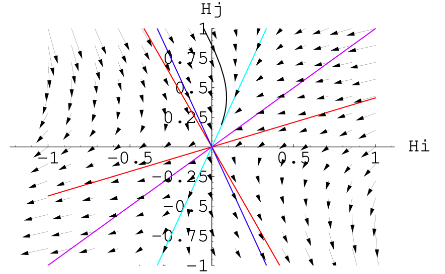
Figure 4: Cosmological flow in the presence of a condensate of winding strings along direction $i$, for $D=3,\mu=1/2$. The axes denote the Hubble parameters of the compact direction $i$ and non-compact directions $j$ in 11D Einstein frame. The dark blue line is the vanishing locus for the Hubble parameter of the direction $i$ in 10D string frame, i.e. $H_{i}+(H_{k}/2)=0$. The purple line is the vanishing locus for the Hubble parameter for the 11th direction $H_{k}$, obtained from Eq. (5.14). The trajectory shown in black corresponds to a bounce of the compact direction $i$ both in 11D Einstein and 10D string frame. It asymptotes to the clear blue line, corresponding to the fixed point $O$.

In order to describe the physics in the string frame, recall that $1/l_{s}^{2}=a_{k}/l_{M}^{3}$ and $g_{s}=(a_{k}/l_{M})^{3/2}$, so that the size of directions $i$ and $j$ in string units are $a_{i}a_{k}^{1/2}$ and $a_{j}a_{k}^{1/2}$, respectively. The dilaton thus appears to be continuously growing to infinity at late times, while the direction $i$ undergoes a bounce in the string frame as well, much before the bounce in the M-theory takes place.

It should however be noted that the class of bouncing solutions that we found cannot be smoothly connected to a Milne geometry in the past, since it would require an initial condition $(|H_{j}|,|H_{k}|)\ll|H_{i}|<1$ outside the basin of attraction for which the bounce occurs.

5.1.4 Condensation of Long Strings in the Rindler Regions

Finally, we would like to discuss the effect of the condensation of winding strings from the point of view of an observer in the Rindler region. The strings are now long strings stretching from radial infinity towards the origin, and are expected to deform the geometry. The Einstein equations can be obtained simply by analytic continuation $T\to ir$, $a_{1}(T)\to ib(r)$, leading to a metric and energy-momentum tensor

$$ds^{2}=dr^{2}-b^{2}(r)d\eta^{2}+c^{2}(r)dx_{j}^{2}\ ,\quad T_{rr}=-\frac{{\cal T}_{2}}{c^{D-1}},\ \ T_{\eta\eta}={\cal T}_{2}\frac{b^{2}}{c^{D-1}}$$ (117)

The main point to observe is a change of sign in the equation of motion (104) for the volume of space-time $bc^{D-1}$,

$$H^{\prime}=-H^{2}+\frac{D+1}{D-1}p\ ,\quad p=\frac{{\cal T}_{2}}{c^{D-1}}$$ (118)

where now $H=(b^{\prime}/b)+(D-1)(c^{\prime}/c)$ and the prime denotes the radial derivative $d/dr$. The effect of long strings in the Rindler region is thus to precipitate the appearance of the singularity $H\to-\infty$. By analytic continuation, this is consistent with the observation that short strings in the Milne region tend to delay the appearance of the singularity.

5.2 Deformations of Misner Space

In the previous subsections, we have shown that a bounce could indeed be induced by the condensation of winding strings, at least for a low transverse dimensionality. In this Section, we will postulate that the Milne geometry is already resolved by the condensation of winding strings and some other mechanism, and study the production rate of winding strings in more general geometries,

$$ds^{2}=-dT^{2}+a^{2}(T)d\theta^{2}+dx_{i}^{2}$$ (119)

Of course, unless $a(T)$ is linear in $T$, such a metric is not a solution of string theory at tree-level, but we expect that (119) is a mean-field description should become on-shell upon including a time-dependent dilaton profile or Fischler-Susskind counterterms, to account for one-loop back-reaction. We assume that $a^{2}(T)$ is even under time reversal, and $a(T)$ is analytic on the real $T$ axis. The metric can then be continued into a Rindler-like regions with time-independent metric

$$ds^{2}=dr^{2}-b^{2}(r)d\eta^{2}+dx_{i}^{2}$$ (120)

with $a(ir)=ib(r)$ is a real and even function of $r$. Note that if $a(T)$ is bounded, $b(r)$ will diverge at some point; this is for example the case of the two-dimensional black hole geometry [41, 11],

$$a(T)=\tanh(\beta T)\ ,\quad b(r)=\tan(\beta r)$$ (121)

On the other hand, even if $a(T)$ is analytic on the real axis, it may have cuts on the imaginary axis, as for example in

$$a(T)=\sqrt{(\beta T)^{2}+\Delta^{2}}\ ,\quad b(r)=\sqrt{(\beta r)^{2}-\Delta^{2}}$$ (122)

with $\Delta>0$ real. In this case, one should retain only the disconnected regions $r<-\Delta$ and $r>\Delta$, which have Lorentzian signature. While the Milne region is now regular, the singularities at $r=\pm\Delta$ in the Rindler regions are now genuine curvature singularities (not to mention the deficit angle introduced by the compactness of $\theta$). This is the geometry which seems to be favored by our qualitative analysis in the previous subsection.

One may also envisage

$$a(T)=\sqrt{(\beta T)^{2}-\Delta^{2}}\ ,\quad b(r)=\sqrt{r^{2}+\Delta^{2}}$$ (123)

which does not satisfy the analyticity condition on the real axis. The two cosmological regions are now disconnected and singular, while the two Rindler regions are connected by a regular throat.

5.2.1 Milne Regions

Let us first consider the dynamics of winding strings in the Milne regions. We choose a gauge such that $\eta(\tau,\sigma)=w\sigma$ and restrict ourselves to configurations where the time coordinate $T(\tau)$ is a function of world-sheet time only. The world-sheet Hamiltonian for $T$ is then given by a simple generalization of (47):

$$L_{0}+\bar{L}_{0}=\frac{1}{a(T)}\partial_{T}~{}a(T)~{}\partial_{T}+\frac{1}{4}w^{2}a^{2}(T)+\frac{J^{2}}{a^{2}(T)}$$ (124)

We recognize in (128) the standard $p_{L}^{2}+p_{R}^{2}$ contribution to $L_{0}+\bar{L}_{0}$ for a compact boson of radius $a(r)$. For $w=0$, this is simply the Laplacian in the deformed geometry (119). This operator has the wrong sign for the kinetic term, but since we are only interested in states with a fixed eigenvalue $-\mu^{2}=-(M^{2}+\tilde{M}^{2})/2$, we may simply consider its opposite. In order to obtain a canonical kinetic term, it is useful to change variables to $x=\int dT/a(T)$, and rewrite the opposite of (124) as a Schrödinger equation $-\partial_{x}^{2}+V(x)=0$ with potential

$$V(x)=-\frac{1}{4}w^{2}a^{4}(T)-\mu^{2}a^{2}(T)-J^{2}=\frac{M^{2}\tilde{M}^{2}}{w^{2}}-\left(\frac{M^{2}+\tilde{M}^{2}}{2w}+\frac{w}{2}a^{2}(T)\right)^{2}$$ (125)

This potential is always negative, and has a maximum when $a^{\prime}(T)=0$; it is unbounded from below if the radius $a(T)$ decompactifies at $T=\pm\infty$ as in the Misner universe case. The potential $V(x)$ is finite even at singular points where $a(T)=0$. Singular points $T_{0}$ where $a(T)$ vanishes at least linearly are at infinite distance in the $x$ metric, leading to disconnected Schrödinger problems on the real $x$-axis for each of the regions $T<T_{0}$ and $T>T_{0}$; the appropriate continuation between the two requires evolving the wave function from the “past Milne region” $T<T_{0}$ into the Rindler patches, and then back into the “future Milne region” $T>T_{0}$. Points where $a(T)$ vanishes less than linearly on the other hand lead to a smooth Schrödinger problem, where trajectories with vanishing mass and angular momentum barely graze the top of the potential.

Let us now assume that the production of winding strings, or some other mechanism, has resolved the cosmological singularity and leads to a nowhere vanishing profile $a(T)$, as in (122) above. We are thus in a “scattering above a potential barrier” situation (see Figure 5, left). A twisted string coming in from $T=-\infty$ will mostly propagate towards $T=+\infty$; part of its wave function however will be reflected back towards $T=-\infty$: as in the Schwinger effect, this can be interpreted as stimulated annihilation of the twisted string. The reflection coefficient can be computing by approximating the potential around $x=0$ by an inverted harmonic oscillator,

$$V(x)=V_{0}-\frac{1}{2}kx^{2}+O(x^{4})\ ,\quad k=\beta^{2}\Delta^{2}(2\mu^{2}+\Delta^{2}w^{2})$$ (126)

leading to a reflection coefficient (e.g. [42], chap.50, ex 4)

$${\cal R}\sim\frac{1}{1+e^{-2\pi V_{0}/\sqrt{k}}}$$ (127)

This is also the spontaneous production rate of twisted strings. At large winding number, the production rate is thus exponentially suppressed as $R\sim\exp(-\pi\frac{w\Delta^{2}}{2\beta})$, in marked improvement from the unresolved Misner geometry. Removing the regulator $\Delta$ at finite $w$ also leads to a vanishingly small reflection coefficient ${\cal R}\sim\exp(-\pi J^{2}\sqrt{2}/\beta\Delta\mu)$, as expected in the Misner limit.

Finally, we note that the classical potential in the $T$ variable, $V(x)/a^{2}(T)$, has only a local minimum at $T=0$, while the true maxima lie at $a^{2}(T)=2|j|/w$ whenever $w<2|j|/\Delta^{2}$. The physical meaning of these off-shell states is unclear.

Figure 5: Potential $V$ controling the production of winding strings in the deformed geometry (122). Left: potential for a winding string in the Milne region, plotted w.r.t. to the flat coordinate $x$. Right: potential for a winding string in the Rindler region, plotted w.r.t. to the flat coordinate $y$. In either case, the horizontal line denotes the (physical) zero energy level. In the Rindler case, the intermediate region has Euclidean signature.

5.2.2 Rindler Regions

Let us now turn to the dynamics of winding strings in the Rindler region. Restricting to configurations with $\eta(\tau,\sigma)=w\sigma$ and $r(\tau)$ is a function of world-sheet time only, the world-sheet Hamiltonian for $r$ is then given by a simple generalization of (47):

$$L_{0}+\bar{L}_{0}=-\frac{1}{b(r)}\partial_{r}~{}b(r)~{}\partial_{r}-\frac{1}{4}w^{2}b^{2}(r)-\frac{J^{2}}{b^{2}(r)}\ ,$$ (128)

equated to $-\mu^{2}=-(M^{2}+\tilde{M}^{2})/2$ by the Virasoro condition. Again, it is useful to change variables to $y=\int dr/b(r)$, leading to a Schrödinger equation $-\partial_{y}^{2}+V(y)=0$ with potential

$$V(y)=-\frac{1}{4}w^{2}b^{4}(r)+\mu^{2}b^{2}(r)-J^{2}=\frac{M^{2}\tilde{M}^{2}}{w^{2}}-\left(\frac{M^{2}+\tilde{M}^{2}}{2w}-\frac{w}{2}b^{2}(r)\right)^{2}$$ (129)

Despite the apparent singularity of the wave equation (128) when $b(r)=0$, the Schrödinger equation based on the potential $V(y)$ is in fact regular (see [43] for an analogous statement in black hole geometries). If $b(r)$ vanishes linearly or faster at $r=r_{0}$, as in the Misner case, the proper distance between the two sides of the singularity is infinite in the $y$ coordinate. In contrast to the Milne regions, these two regions are causally disconnected and the Hilbert space factorizes into a tensor product of states on each side. As we have seen in Section 3, on either side of the singularity, the particles can tunnel between infinity and $r=r_{0}$, leading to production of pairs of long and short strings.

Let us now investigate the case where $b(r)$ is deformed as in (122) with $\Delta^{2}>0$ (see Figure 5, right). The vanishing locus of $b(r)$ now splits into splits into two points at $r=\pm\Delta/\beta$, which are at finite distance in the $y$ coordinate. For $r>r_{0}=\Delta/\beta$, one may choose $r=(\Delta/\beta)\cosh\beta y$ with $y>0$. The potential has a quadratic minimum with negative energy at $y=0$,

$$V=-J^{2}+(\Delta\beta\mu)^{2}y^{2}+O(y^{2})\ ,\quad y>0$$ (130)

then reaches a maximum with positive energy at $y_{1}$ given by $\sinh y_{1}=\sqrt{M^{2}+\tilde{M}^{2}}/(w\Delta)$, such that

$$V=\frac{\mu^{4}}{w^{2}}-J^{2}-\frac{2\beta^{2}\mu^{2}(2\mu^{2}+\Delta^{2}w^{2})}{w^{2}}(y-y_{1})^{2}+O[(y-y_{1})^{3}]$$ (131)

before dropping to negative values at large $y$. There is thus tunneling between the $y<y_{1}$ and $y>y_{1}$ regions, just as in the unresolved Misner geometry. The tunneling rate can be computed as before by approximating the local maximum with an inverted harmonic oscillator. In the large $w$ limit, it is easy to see that the reflection rate reaches a finite value,

$$R\sim\frac{1}{1+\exp\left[\pi\frac{J^{2}\sqrt{2}}{\beta\Delta\mu}\right]}$$ (132)

which goes to zero when the regulator $\Delta$ is removed.

However, the point $y=0$ is now at finite distance, and one needs to enforce boundary conditions there. A natural prescription is to continue solving the wave equation, now in the Euclidean region $-\Delta/\beta<r<\Delta/\beta$. More precisely, in the region where $b(r)$ is imaginary we define the real coordinate $dy=idr/b(r)$. The wave equation can now be written as a Schrödinger equation $+\partial_{y}^{2}+V(y)=0$, with now $r=(\Delta/\beta)\cos(\beta y)$. In other words, the potential governing the $y$ evolution in the $-\Delta/\beta<r<\Delta/\beta$ is now $-V$. Since it is negative, we are again in a classically forbidden region. Finally, we revert to Lorentzian evolution in the $r<-\Delta/\beta$ region, corresponding to the left Rindler patch. Altogether, we thus find an exponentially suppressed coupling between the right and left Rindler patches, through an intermediate region of Euclidean signature. The resulting production rates of long and short strings in each of the Rindler regions can be computed in a reliable way by standard WKB techniques.

If on the other hand the deformation corresponds to (123), the wave equation becomes regular for all values of $y$, and allows propagation between $y>0$ and $y<0$, covering the whole real $r$ axis. This situation is analogous to the Milne region discussed in Section 5.2.1. The turning points at zero energy lie at $b^{2}=(M\pm\tilde{M})^{2}/(w^{2})$ and disappear at large $w$, where the motion between $y>0$ and $y<0$ becomes classically allowed. There is nevertheless pair production in this case as well, which can be computed as above by approximating the potential by an inverted harmonic well.

6 Conclusion

In this paper, we have discussed the behavior of closed strings in Misner space, a toy example of a cosmological singularity where string theory can in principle be solved. By studying semiclassically the tree-level spectrum and one-loop amplitude, we have found several features which we believe should be of more general validity:

• The usual divergences in the energy-momentum tensor in field theory are more acute in string theory, due to the existence of Regge trajectories with arbitrarily high spins. On the other hand, local expectation values of the energy-momentum tensor are not directly observable, and the integrated free energy may still be finite.

• Winding string production can be understood at a semi-classical level as tunneling under the barrier in regions with compact time, or scattering over the barrier in cosmological regions. In general, it can be computed as a tree-level two-point function in an appropriate basis depending on the choice of vacuum. In our free field example, it just reduces to the overlap of the zero-mode wave functions.

• In the presence of CTC, there may exist closed string configurations wrapping the time-like direction. Such strings are better viewed as possibly infinite static stretched strings. Due to the peculiar causal structure of the induced metric on the world-sheet, it may be more appropriate to quantize them with respect to the world-sheet compact coordinate $\sigma$ rather than $\tau$.

• Long strings living the whiskers and short strings living in the cosmological region have a non-trivial two-point function. It is therefore not legitimate to truncate the space to the cosmological region only.

• In the presence of a cosmological singularity with compact transverse space, we expect a production of winding states (strings or D-branes). Their effect on the geometry should be analogous to that of a positive cosmological constant. If sufficient, it may prevent the instabilities towards large black hole formation.

• In addition to the divergences appearing in the energy-momentum tensor of untwisted fields, the production rate for winding strings diverges at large winding number. It should be possible to determine the resolved geometry self-consistently so that the divergences at one-loop cancel those at tree-level. Hopefully, there should exist a regime of parameters where higher loops can consistently be neglected.

It is our hope that the Lorentzian orbifold can teach us some of the new physics which will be needed to understand gravitational back-reaction in the vicinity of cosmological singularities.

Acknowledgments: We are grateful to I. Affleck, O. Bergman, R. Brustein, B. Craps, B. Durin, A. Konechny, R. Parentani, D. Reichmann, K. Schleich, G. Semenoff, K. Skenderis, A. Strominger, M. van Raamsdonk and E. Verlinde for useful discussions and comments. The three authors are indebted to the Aspen Center for Physics for providing a stimulating atmosphere which lead to this collaboration. B. P. and M . R. are grateful to the Weizmann Institute for hospitality during part of this work. M.B. is grateful to KITP and Ecole Polytechnique for their hospitality during part of this work. The work of M.B. is supported by Israeli Academy of Science Centers of Excellence program, by the Minerva Foundation, by the Harold Blumenstein Foundation and by EEC grant RTN-2000-001122. The work of M.R. is supported by NSERC discovery grant.

References

- [1] R. H. Brandenberger and C. Vafa, “Superstrings In The Early Universe,” Nucl. Phys. B 316 (1989) 391.
- [2] A. E. Lawrence and E. J. Martinec, “String field theory in curved spacetime and the resolution of spacelike Class. Quant. Grav. 13 (1996) 63 [arXiv:hep-th/9509149].
- [3] S. S. Gubser, “String production at the level of effective field theory,” Phys. Rev. D 69 (2004) 123507 [arXiv:hep-th/0305099].
- [4] A. J. Hamilton, D. Kabat and M. K. Parikh, “A First-quantized formalism for cosmological particle production,” JHEP 0407 (2004) 024 [arXiv:hep-th/0311180].
- [5] C. R. Nappi and E. Witten, “A Closed, expanding universe in string theory,” Phys. Lett. B 293, 309 (1992) [arXiv:hep-th/9206078].
- [6] J. Khoury, B. A. Ovrut, N. Seiberg, P. J. Steinhardt and N. Turok, “From big crunch to big bang,” Phys. Rev. D 65 (2002) 086007 [arXiv:hep-th/0108187].
- [7] N. A. Nekrasov, “Milne universe, tachyons, and quantum group,” arXiv:hep-th/0203112.
- [8] S. Elitzur, A. Giveon, D. Kutasov and E. Rabinovici, “From big bang to big crunch and beyond,” JHEP 0206, 017 (2002) [arXiv:hep-th/0204189];
- [9] H. Liu, G. Moore and N. Seiberg, “Strings in a time-dependent orbifold,” JHEP 0206, 045 (2002) [arXiv:hep-th/0204168]; “Strings in time-dependent orbifolds,” JHEP 0210, 031 (2002) [arXiv:hep-th/0206182].
- [10] L. Cornalba and M. S. Costa, “A New Cosmological Scenario in String Theory,” Phys. Rev. D 66, 066001 (2002) [arXiv:hep-th/0203031].
- [11] B. Craps, D. Kutasov and G. Rajesh, “String propagation in the presence of cosmological singularities,” JHEP 0206, 053 (2002) [arXiv:hep-th/0205101];
- [12] M. Fabinger and J. McGreevy, “On smooth time-dependent orbifolds and null singularities,” JHEP 0306, 042 (2003) [arXiv:hep-th/0206196].
- [13] M. Berkooz, B. Craps, D. Kutasov and G. Rajesh, “Comments on cosmological singularities in string theory,” JHEP 0303 (2003) 031 [arXiv:hep-th/0212215].
- [14] M. Berkooz, and B. Pioline, “Strings in an electric field, and the Milne universe,” JCAP 0311 (2003) 007 [arXiv:hep-th/0307280].
- [15] B. Craps and B. A. Ovrut, “Global fluctuation spectra in big crunch / big bang string vacua,” Phys. Rev. D 69 (2004) 066001 [arXiv:hep-th/0308057].
- [16] C. W. Misner, in Relativity Theory and Astrophysics I: Relativity and Cosmology, edited by J. Ehlers, Lectures in Applied Mathematics, Vol. 8 (American Mathematical Society, Providence, 1967), p. 160.
- [17] A. Lawrence, “On the instability of 3D null singularities,” JHEP 0211, 019 (2002) [arXiv:hep-th/0205288]; G. T. Horowitz and J. Polchinski, “Instability of spacelike and null orbifold singularities,” Phys. Rev. D 66, 103512 (2002) [arXiv:hep-th/0206228].
- [18] J. S. Schwinger, “On Gauge Invariance And Vacuum Polarization,” Phys. Rev. 82 (1951) 664.
- [19] J. D. Grant, “Cosmic strings and chronology protection,” Phys. Rev. D 47 (1993) 2388 [arXiv:hep-th/9209102].
- [20] F. Cooper, J. M. Eisenberg, Y. Kluger, E. Mottola and B. Svetitsky, “Particle production in the central rapidity region,” Phys. Rev. D 48, 190 (1993) [arXiv:hep-ph/9212206].
- [21] N.D. Birrell and P.C.W. Davies, Quantum Fields in Curved Space, Cambridge, UK: Univ. Pr
- [22] L. Cornalba, M. S. Costa and C. Kounnas, “A resolution of the cosmological singularity with orientifolds,” Nucl. Phys. B 637, 378 (2002) [arXiv:hep-th/0204261].
- [23] L. Cornalba and M. S. Costa, “On the classical stability of orientifold cosmologies,” Class. Quant. Grav. 20 (2003) 3969 [arXiv:hep-th/0302137].
- [24] N. Drukker, B. Fiol and J. Simon, “Goedel’s universe in a supertube shroud,” Phys. Rev. Lett. 91 (2003) 231601 [arXiv:hep-th/0306057].
- [25] D. Israel, “Quantization of heterotic strings in a Goedel/anti de Sitter spacetime and chronology protection,” JHEP 0401 (2004) 042 [arXiv:hep-th/0310158].
- [26] C. Gabriel and P. Spindel, “Quantum charged fields in Rindler space,” Annals Phys. 284 (2000) 263 [arXiv:gr-qc/9912016].
- [27] M. Berkooz, B. Durin, B. Pioline and D. Reichmann, ”Closed strings in misner space: stringy fuzziness with a twist”, arXiv: hep-th/0407216.
- [28] A. Strominger and T. Takayanagi, “Correlators in timelike bulk Liouville theory,” Adv. Theor. Math. Phys. 7 (2003) 369 [arXiv:hep-th/0303221].
- [29] S. W. Hawking, “The Chronology protection conjecture,” Phys. Rev. D 46, 603 (1992).
- [30] E. S. Fradkin and A. A. Tseytlin, “Nonlinear Electrodynamics From Quantized Strings,” Phys. Lett. B 163, 123 (1985); A. Abouelsaood, C. G. Callan, C. R. Nappi and S. A. Yost, “Open Strings In Background Gauge Fields,” Nucl. Phys. B 280, 599 (1987). C. P. Burgess, “Open String Instability In Background Electric Fields,” Nucl. Phys. B 294, 427 (1987).;
- [31] C. Bachas and M. Porrati, “Pair Creation Of Open Strings In An Electric Field,” Phys. Lett. B 296, 77 (1992) [arXiv:hep-th/9209032].
- [32] I. K. Affleck and N. S. Manton, “Monopole Pair Production In A Magnetic Field,” Nucl. Phys. B 194, 38 (1982); I. K. Affleck, O. Alvarez and N. S. Manton, “Pair Production At Strong Coupling In Weak External Fields,” Nucl. Phys. B 197, 509 (1982).
- [33] N. K. Nielsen and P. Olesen, “An Unstable Yang-Mills Field Mode,” Nucl. Phys. B 144 (1978) 376.
- [34] J. R. David, “Unstable magnetic fluxes in heterotic string theory,” JHEP 0209 (2002) 006 [arXiv:hep-th/0208011].
- [35] W. A. Hiscock and D. A. Konkowski, “Quantum Vacuum Energy In Taub - Nut (Newman-Unti-Tamburino) Type Cosmologies,” Phys. Rev. D 26 (1982) 1225.
- [36] S. V. Sushkov, “Chronology protection and quantized fields: Complex automorphic scalar Class. Quant. Grav. 14 (1997) 523 [arXiv:gr-qc/9509056].
- [37] J. M. Maldacena, H. Ooguri and J. Son, “Strings in AdS(3) and the SL(2,R) WZW model. II: Euclidean black hole,” J. Math. Phys. 42, 2961 (2001) [arXiv:hep-th/0005183].
- [38] E. M. Lifshitz and I. M. Khalatnikov, “Investigations In Relativistic Cosmology,” Adv. Phys. 12, 185 (1963); V. A. Belinsky, I. M. Khalatnikov and E. M. Lifshitz, “Oscillatory Approach To A Singular Point In The Relativistic Cosmology,” Adv. Phys. 19, 525 (1970); V. a. Belinsky, I. m. Khalatnikov and E. m. Lifshitz, “A General Solution Of The Einstein Equations With A Time Singularity,” Adv. Phys. 31, 639 (1982).
- [39] A. A. Tseytlin and C. Vafa, “Elements of string cosmology,” Nucl. Phys. B 372 (1992) 443 [arXiv:hep-th/9109048].
- [40] C. Molina-Paris and M. Visser, “Minimal conditions for the creation of a Friedman-Robertson-Walker universe Phys. Lett. B 455, 90 (1999) [arXiv:gr-qc/9810023].
- [41] R. Dijkgraaf, H. Verlinde and E. Verlinde, “String propagation in a black hole geometry,” Nucl. Phys. B 371 (1992) 269.
- [42] L. Landau and E. Lifschitz, Mechanique Quantique, Editions Mir, Moscou; Section 50, Exercice 4.
- [43] A. Giveon, B. Kol, A. Ori and A. Sever, “On the resolution of the time-like singularities in Reissner-Nordstroem and negative-mass Schwarzschild,” arXiv:hep-th/0401209.