AdS/CFT description of D-particle decay

Abstract

Unstable D-particles in type-IIB string theory correspond to sphaleron solutions in the dual gauge theory. We construct an explicit time-dependent solution for the sphaleron decay on $S^{3}\times\mathbb{R}$, as well as the coherent state corresponding to the decay product. We develop a method to count the number of bulk particles in the AdS/CFT setup. When applied to our coherent state, the naive number operator $\hat{O}_{J}^{\dagger}\hat{O}^{\phantom{\dagger}}_{J}$ is shown to be inappropriate, even in the large-$N$ limit. The reason is that the final state consists of a large number of particles. By computing all probabilities for finding multi-particle states in the coherent state, we deduce the bulk particle content of the final state of the sphaleron decay. The qualitative features of this spectrum are compared with the results expected from the gravity side, and agreement is found.

I Introduction and summary

The spectrum of type-IIB string theory contains, apart from the stable BPS and non-BPS states, also a wide variety of unstable D-branes. These unstable branes contain a tachyon field on their world-volume, and the condensation of this field corresponds to the decay of the brane. Recently, a lot of progress has been made in understanding the dynamical aspects of the decay of unstable branes. Most of the analysis was performed directly using boundary conformal field theory in flat space, initiated by Sen’s construction of the boundary states for decaying D-branes Sen (2002), or by using the $c=1$ matrix model for the description of the decay of D-branes in 1+1 dimensional string theory McGreevy and Verlinde (2003). In the present paper we would like to study the problem of decaying branes in the set-up of the “standard” AdS/CFT correspondence.

As was argued by Harvey et al. Harvey et al. (2000), the unstable D-branes in string-theory are equivalents of “sphalerons”: they are unstable solutions located at a saddle point of the potential in configuration space, at the top of a non-contractible loop Manton (1983). In the context of the AdS/CFT conjecture, this correspondence between unstable D-branes and sphalerons is in fact even more direct. It has been argued by Drukker et al. Drukker et al. (2000) that the existence of sphaleronic saddle points in the potential of the theories on both sides is a feature which is preserved when going from weak to strong coupling, despite the fact that the precise form of the potential receives quantum corrections. The unstable D-particles of string theory are then in precise correspondence with known sphaleron solutions of the dual gauge theory. Kinematical aspects of this correspondence were investigated in detail in Drukker et al. (2000).

In the present paper, we will analyse dynamical aspects of this correspondence. Our analysis consists of three parts. First, we will construct the classical solution of the decaying sphaleron, and obtain a quantum mechanical description of the final stage of this decay using a coherent state. We then develop the formalism to count the number of bulk particles into which this final state decomposes. In the last part, we apply this formalism to a concrete case at finite $N$ and extract qualitative features of the decay process. Although the whole process is highly non-supersymmetric, and thus expected to be subject to quantum corrections, we will see that there are indeed qualitative features which agree with known results derived on the string theory side.

The dual gauge theory system is studied by considering a time dependent solution of the decaying sphaleron on the three-sphere. We are able to find an analytic, classical solution for the spherically symmetric decay channel of the sphaleron. While the non-abelian character of the gauge theory (i.e. the non-vanishing coupling) is crucial for the existence of the sphaleron solution near the top of the potential, it turns out that our solution abelianises near the bottom of the potential valley (i.e. it is a solution to the free Yang-Mills equations of motion on the sphere). This allows us to construct a coherent state corresponding to the final product of the sphaleron decay. This coherent state should be dual to the gas of closed string particles which is the decay product of an unstable D-particle.

In order to make a link with calculations on the gravity side, we then calculate the “number operators” in this coherent state $|c\rangle$ for various single trace operators $\hat{O}_{J}$ which are dual to closed string particles. There are two subtle points in this procedure. One is related to the fact that in gravity calculations one uses the “standard” notion of particles in the bulk as (angular) momentum eigenstates, and calculates emission amplitudes for these particles. Hence, in order to make a comparison with gravity possible, we cannot directly use the AdS/CFT correspondence in position space. Instead, we first have to construct boundary operators that are dual to bulk angular momentum eigenstates. To construct these operators one projects the composite operators onto eigen angular momentum operators, by multiplying them with the appropriate tensorial spherical harmonics and integrating over the sphere. This construction is explained in the section II.3 and further illustrated on an explicit example in appendix V.1.

The second subtlety in counting particles in the coherent state is related to the fact that the operators $\hat{O}_{J}$ which create elementary bulk particles are, from the point of view of the gauge theory, composite rather than elementary operators. The naive number operator $\hat{O}^{\dagger}_{J}\hat{O}^{\phantom{\dagger}}_{J}$ turns out to be inappropriate; we will see that this is because it only behaves as a counting operator when both $N\rightarrow\infty$ and the number of particles $p$ in the state satisfies $p\ll N$. Therefore, in order to count the number of particles corresponding to an operator $\hat{O}_{J}$, one needs to calculate the probabilities ${\cal P}_{p}$ for finding a $p$-particle state individually. Since $\hat{O}_{J}$ particles can appear in combination with any arbitrary other (multi-particle) operator $\hat{O}_{K}$, the expression for finding a $p$-particle $\hat{O}_{J}$ state is

$${\cal P}_{p}=\sum_{\hat{O}_{K}}\frac{\displaystyle\left|\Big{\langle}(\hat{O}_{J})^{p}\hat{O}_{K}\,\Big{|}\,c\Big{\rangle}\right|^{2}}{\displaystyle\Big{\langle}(\hat{O}_{J})^{p}\hat{O}_{K}\,\Big{|}\,(\hat{O}_{J})^{p}\hat{O}_{K}\Big{\rangle}\langle c|c\rangle}\,.$$ (1)

To see why computing (1) is hard, consider the simplest terms in the sum, when $\hat{O}_{K}$ is just the identity operator. This term is

$$\frac{\displaystyle\left|\Big{\langle}(\hat{O}_{J})^{p}\,\Big{|}\,c\Big{\rangle}\right|^{2}}{\displaystyle\Big{\langle}(\hat{O}_{J})^{p}\,\Big{|}\,(\hat{O}_{J})^{p}\,\Big{\rangle}\langle c|c\rangle}=\frac{\Big{|}(O_{J})^{p}\,\langle 0|c\rangle\Big{|}^{2}}{p!\left(1+\frac{b(p,J)}{N^{2}}+\ldots\right)}\,,$$ (2)

where $O_{J}$ without a hat denotes the (positive frequency part of the) classical expectation value of the operator $\hat{O}_{J}$. When $b\ll N$, the expression (1) can be summed, yielding the result one would obtain using the naive number operator. However, as indicated, the coefficient $b$ in the denominator depends on $p$ and $J$, and for large $p$ it becomes comparable to $N^{2}$. This invalidates the large-$N$ approximation for the sum. Closer analysis of our coherent state shows that, due to the non-perturbative character of the initial gauge configuration, the classical expectation values of the operator $\hat{O}_{J}$ in the coherent state are very large. The maximal term in (1) is attained for large $p$, which grows so fast with $N$ that one cannot neglect $1/N^{2}$ and higher order corrections in the denominator. Moreover, summing all planar contributions does not yield a good approximation either.

This makes the problem of calculating the energy distribution in the outgoing state very hard to do analytically. In section III.3 we instead adopt a Monte-Carlo method in order to compute the state norms, and subsequently evaluate the sum (1) for all operators in the U(4) case. We show that, as expected from string calculations, particles in the final state are suppressed as their mass increases. We also show that, had one not taken the full norms in (1) into account, one would incorrectly find that the energy distribution increases for more and more massive particles. This is essentially due to the fact that classical expectation values for all operators grow with their dimension.

Our results agree in a qualitative sense with results from previous calculations on the gravity side. The calculations on the gravity side have already been performed in the literature for decaying D-branes in flat space Lambert et al. (2003). To compare these to the gauge theory calculations, we “embed” these results in the AdS space. A priori, there is no reason to expect that the flat space results of the decay should be valid for branes in an AdS background. However, since the D-particles in question are fully localised in the bulk space, one expects that the flat space results should carry over, at least when the radius of the AdS is large. There are two properties of the spectrum of the decaying brane that we can compare with the dual gauge theory calculation. The first property of the spectrum is constrained by the symmetries of the system, and concerns emission amplitudes for the states on the leading Regge trajectory. By slightly refining the calculation of Lambert et al. (2003) in section III.2 we find that all emission amplitudes for these states are zero. The same result is then separately recovered on the gauge theory side by evaluating the number operator for the corresponding dual composite operators.

More important is a second property of the spectrum, observed in Lambert et al. (2003), which reflects genuine dynamical features of the decay. There is strong evidence Sen (2002); Lambert et al. (2003) that the open strings decay fully into closed string states, i.e. that there is no open string remnant left after the decay. This conclusion is also supported by the matrix model calculations of McGreevy and Verlinde (2003). As shown in Lambert et al. (2003), the emission amplitudes are exponentially suppressed with the level of the emitted string, at least for high levels (however, due to the exponential growth of the available states, most of the energy of the brane gets transferred into a high-density cloud of very massive closed string states). By studying the dual gauge model we discover the same qualitative feature: a suppression of higher-mass string states in the decay product.

II Decaying sphalerons in AdS/CFT

II.1 Classical instability of the sphaleron on $S^{3}\times\mathbb{R}$

The first step in our analysis is to give a detailed description of the decaying sphaleron on the gauge theory side. Whereas the sphaleron solution on $\mathbb{R}^{4}$ found by Klinkhamer and Manton Klinkhamer and Manton (1984) is very complicated and not known analytically, the situation is much simpler on $S^{3}\times\mathbb{R}$. Not only is the solution known in this case, but one can also find an analytic description of the classical decay of this metastable state.

Following Drukker et al. Drukker et al. (2000), one can get a sphaleron solution on $S^{3}\times\mathbb{R}$ by starting from the instanton solution on $\mathbb{R}^{4}$. The latter is given by

$$A_{\mu}=f(r)(\partial_{\mu}U)U^{\dagger},\quad\quad U=\frac{x^{\mu}\sigma_{\mu}}{r},\quad\quad r^{2}=x_{0}^{2}+x_{i}^{2}\,,$$ (3)

where $f=r^{2}/(r^{2}+a^{2})$. This function interpolates between two pure gauge configurations (i.e. the two vacua) $f(r=0)=0$ and $f(r=\infty)=1$. When $f(r)=1/2$, the system is at the top of the potential barrier. By taking $f=1/2$ everywhere one gets a singular solution to the equation of motion on $R^{4}$, which is the so-called “meron”. The $f=1/2$ solution is, however, also a solution on $S^{3}\times\mathbb{R}$, since this manifold can be conformally mapped to $\mathbb{R}^{4}$ and Yang-Mills theory in four dimensions is conformally invariant. The solution obtained in this way is the Euclidean version of the “sphaleron”, and is non-singular. The Lorentzian version is the same, since the time component of the potential of the sphaleron is zero; the solution is completely time-independent.

We want to study the decay of the sphaleron, and we restrict to those modes which preserve the spatial homogeneity of the initial sphaleron configuration. This is because we want to look at the decay of the D-particle which sits at the “origin” of the anti-de-Sitter space and is projected in the same way to all points on the boundary. In other words, we only allow for time dependence, so that energy-momentum tensor should be of the form

$$T_{00}=g(t)\,,\quad\quad T_{ij}=h(t)g_{ij}\,,$$ (4)

where $g_{ij}$ is the metric on $S^{3}$. So the ansatz we make is

$$A=f(t)\,\Sigma^{i}\sigma_{i}\,,$$ (5)

where $\Sigma^{i}$ are the three left-invariant one-forms. The energy momentum tensor,

$$T_{\mu\nu}=\operatorname{Tr}(F_{\mu\rho}F_{\nu\sigma}g^{\rho\sigma})-\frac{1}{4}g_{\mu\nu}\operatorname{Tr}(F^{2})$$ (6)

reduces for our ansatz to the desired form (4) with the functions $g$ and $h$ given by

$$g(t) =-\frac{3}{2}R^{2}\dot{f}^{2}-6f^{2}(1-f)^{2}\,,$$ (7)

$$h(t) =-\frac{1}{2}R^{2}\dot{f}^{2}-2f^{2}(1-f)^{2}=-\frac{g(t)}{3}\,.$$

To deduce what is the unknown function $f(t)$ we plug the ansatz into the action and derive the action for this function. The value of the action for our ansatz is

$$S =-\frac{1}{4g_{\text{YM}}^{2}}\int\!{\rm d}t{\rm d}\Omega\,F_{\mu\nu}F^{\mu\nu}$$ (8)

$$=\frac{24\,\operatorname{vol}(S^{3})}{4\,g_{\text{YM}}^{2}}\int\!\frac{{\rm d}t}{R}\left(\frac{R^{2}}{2}\dot{f}^{2}-2f^{2}(1-f)^{2}\right)\,,$$

where $\operatorname{vol}(S^{3})\equiv 2\pi^{2}$ denotes the volume of the unit sphere and $R$ is the radius of $S^{3}$ (also see (73), (77)). The equation of motion for the function $f$ is

$$R^{2}\,\ddot{f}+4f(1-f)(1-2f)=0\,.$$ (9)

This equation can be integrated once, yielding a conserved quantity, namely the energy (i.e. the component $T_{00}=48\operatorname{vol}(S^{3})E$)

$$E=R^{2}\,\dot{f}^{2}+4f^{2}(1-f)^{2}\,.$$ (10)

By introducing a new variable $H(t)$

$$f(t)=\frac{1}{2}(1+H(t))\,,$$ (11)

the expression for energy becomes

$$4E=R^{2}\,\dot{H}^{2}+(1-H^{2})^{2}\,,$$ (12)

which can be further integrated analytically for $E=\tfrac{1}{4}$. There are two solutions, corresponding to the fact that the sphaleron can roll down on either side of the potential, to the vacua with Chern-Simons number one and zero respectively. The final result reads (see figure 1)

$$f_{\pm}(t)=\frac{1}{2}\left(\frac{\pm\sqrt{2}}{\cosh\left(\frac{\sqrt{2}}{R}(t-t_{0})\right)}+1\right)\,.$$ (13)

Figure 1: The functions $f_{\pm}(t)$ of the decaying sphaleron on $S^{3}$ as given in (13), together with the kinetic and potential energy (with normalisation as given in (12) and $R=1$).

One can check that these solutions are indeed solutions to the full equations of motion, not just to the equations obtained from the reduced action. These solutions describe a configuration that starts from the potential maximum at $t=-\infty$ (with zero velocity and acceleration), rolls down one of the two sides of the hill and up the other side, where it arrives at $t=t_{0}$. The minimum of the potential energy (12) is reached when $H^{2}=1$ which corresponds to $t-t_{0}=\pm R\operatorname{arccosh}(\sqrt{2})/\sqrt{2}\approx\pm 0.62\,R$; the evolution is symmetric around $t=t_{0}$.

The periodicity of the whole process is natural from the AdS perspective. Since AdS effectively acts as a box, the cloud of outgoing radiation is refocused to the origin of the space, where it arrives as fine-tuned radiation and “re-builds” the D-particle. In this sense the D-particle never decays, since there is no real dissipation of the energy in the system. However, in the limit of large AdS radius, our flat-space intuition should (at least approximately) hold. A natural point in time, which should be associated to the decayed brane, is the point where the sphaleron has rolled down to the the bottom of the potential, i.e. when all potential energy has been converted to kinetic energy.

The previous construction can easily be generalised to describe the decay of a system of coincident D-particles. The relevant sphaleron configurations have been given by Drukker et al. Drukker et al. (2000). They are obtained by replacing the Pauli matrices in (3) with Clifford algebra generators according to

$$\sigma_{\mu}\rightarrow\gamma_{\mu}=\begin{pmatrix}\sigma_{\mu}&0&\cdots&0\\ 0&\sigma_{\mu}&\cdots&0\\ \vdots&\vdots&\ddots&0\\ 0&0&\cdots&\sigma_{\mu}\end{pmatrix}\,.$$ (14)

This will make the various sphalerons sit in mutually commuting SU(2) factors within U($N$). In this case (9) gets replaced by an independent equation for each of the functions $f_{i}$, and the solutions of those are given by (13) which can differ only by the value of $t_{0}$. In what follows we will restrict to the situations in which all these initial “phases” are the same, i.e. in which all D-particles start to decay at the same time. Since the field strengths will also be block-diagonal, traces of powers of them will decompose as sums of traces of the individual blocks.

II.2 Coherent state description of the sphaleron decay

In order to perform an analysis of the spectrum of the decay in the gauge theory, as a first step one needs to construct a quantum state describing the decayed sphaleron. For that purpose, it is useful to think about the sphaleron decay in the following way. Near the top of the potential, most of the energy of the (perturbed) sphaleron configuration is stored in the potential energy, which arises from the non-linear terms in the Yang-Mills action. Precisely these non-linearities in the action ensure the existence of the sphaleron solution. However, as the sphaleron decays, the potential energy of the sphaleron gets transferred into kinetic energy, and near the bottom of the potential valley all of the energy of the configuration is stored in the kinetic energy. This can be seen most easily by performing a finite gauge transformation (78) on the solution (5) with gauge parameter $\Lambda=U^{\dagger}$. The solution then reduces to

$$A_{\mu}=\tilde{f}(t)\,U^{\dagger}(\partial_{\mu}U)\,,\quad\tilde{f}=f-1\,.$$ (15)

Near the bottom of the potential $\tilde{f}\approx 0$, which means that the derivative part of the field strength, rather than the non-linear (commutator) part, is dominant. The solution becomes solution of the free Yang-Mills equations of motion on $S^{3}\times\mathbb{R}$ (written in the radiation gauge: $A_{0}=\nabla_{i}A^{i}=0$)

$$\Big{(}-\partial_{t}^{2}+\frac{1}{R^{2}}\big{(}\nabla_{S^{3}}^{2}-2\big{)}\Big{)}A^{\text{lin.}}_{i}=0\,.$$ (16)

Indeed, one can easily see that as $t\rightarrow t_{\text{bottom}}$ the solution (15) with $f$ given by (13) is very well approximated by the following solution of the linearised equation of motion (16):

$$A_{i}^{\text{lin.}}=-\frac{1}{4}\sin\left(\frac{2(t-t_{\text{bottom}})}{R}\right)\,U^{\dagger}(\partial_{i}U)\,.$$ (17)

Hence near the bottom of the valley, one can think about the Yang-Mills configuration as dual to a coherent state of non-interacting closed string states which are the product of the D-particle decay. Our goal will then be to determine numbers of various (gravity) “particles” in this final coherent state. What we precisely mean by this will be explained in the next section. Let us first construct this coherent state.

The fact that our solution abelianises near the bottom of the potential valley allows us to write down a coherent state for this configuration (see Cahill Cahill (1974) and Pottinger Pottinger (1978) for related work). In order to do so, we need an expansion of the free Yang-Mills gauge potential in spherical vector harmonics. In the radiation gauge, an expansion is given by (we refer the reader to Hamada and Horata Hamada and Horata (2003) for more on spherical harmonics)

$$A^{ab}_{i}=\sum_{J,y,M}\Big{(}\hat{a}^{ab}_{JMy}\frac{e^{-(2J+1)\tau/R}}{\sqrt{2(2J+1)}}Y^{i}_{JMy}(\phi,\theta,\psi)\\[4.30554pt] +\hat{a}^{\dagger ab}_{JMy}\frac{e^{(2J+1)\tau/R}}{\sqrt{2(2J+1)}}Y^{*i}_{JMy}(\phi,\theta,\psi)\Big{)}\,,$$ (18)

where $M=(m,m^{\prime})$ labels the representations of the simple factors of SO(4)=SU(2)$\times$SU(2) and $y$ sums over the physical polarisation states of the gauge field. We have also introduced matrix indices for the adjoint representation of the U($N$) Lie-algebra. The other indices run over the ranges

$$\begin{aligned} J&\geq\tfrac{1}{2}\,,\\ y&=\pm\tfrac{1}{2}\,,\end{aligned}\quad\begin{aligned} -J-y&\leq\,m\,&&\leq J+y\,,\\ -J+y&\leq\,m^{\prime}\,&&\leq J-y\,.\end{aligned}$$ (19)

After quantisation, the operators $\hat{a}_{lmn}^{\dagger}$ and $\hat{a}_{lmn}$ satisfy the canonical commutation relations

$${}\Big{[}\hat{a}^{ab}_{JMy},\hat{a}^{\dagger cd}_{J^{\prime}M^{\prime}y^{\prime}}\Big{]}=g_{\text{YM}}^{2}\,\delta_{JJ^{\prime}}\delta_{MM^{\prime}}\delta_{yy^{\prime}}\delta^{ad}\delta^{bc}\,.$$ (20)

A coherent state (see Klauder and Skagerstam Klauder and Skagerstam (1985) for more on coherent states and references to the literature) corresponding to the classical configuration given by (13) is constructed by demanding that

$$\hat{a}^{ab}_{JMy}|c\rangle=A^{ab}_{JMy}|c\rangle\,,$$ (21)

where $A_{JMy}$ are the coefficients appearing in the Fourier decomposition of the classical sphaleron configuration, as in (18). In the Coulomb gauge $A_{0}^{ab}=0$ the coherent state can be written as

$$|c\rangle={\cal C}\,\exp\left(g_{\text{YM}}^{-2}\sum_{J,M,y}\operatorname{Tr}\big{(}A_{JMy}\,\hat{a}^{\dagger}_{JMy}\big{)}\right)|0\rangle\,,$$ (22)

The normalisation factor ${\cal C}$ is chosen such that $|c\rangle$ is of unit norm and is given by

$${\cal C}=\exp\Big{(}-\tfrac{1}{2}g_{\text{YM}}^{-2}\operatorname{Tr}\big{(}\sum_{JMy}|A_{JMy}|^{2}\big{)}\Big{)}\,.$$ (23)

A similar construction for the Klinkhamer-Manton sphaleron in Yang-Mills-Higgs theory on $\mathbb{R}^{(3,1)}$ has been discussed by Zadrozny Zadrozny (1992). The state (22) is most natural from the point of view of the gauge theory; we will discuss the possibility of using alternative coherent states at the end of section II.3.

It is important to note that, due to the properties of the vector spherical harmonics in (18), the coherent state (22) has been built from creation operators that excite only physical excitations: the Gauss law constraint is automatically implemented using these operators, since $\nabla\cdot\hat{A}^{\text{free}}=0$ holds as an operator equation. Hence the coherent state (22) is a legitimate state in the Hilbert space of the free theory.

Nevertheless, the state (22) does not yet provide a good description of the system, as it is constructed using the oscillators of the free theory and does not allow for a smooth deformation to the interacting theory. At finite coupling, it does not satisfy the global colour neutrality constraint. This constraint arises because the commutator term in the Gauss law acts as a source, and by integrating the constraint over the $S^{3}$ one finds that this total charge has to vanish. One therefore imposes that the commutator part of the non-abelian constraint vanishes also at zero coupling Sundborg (2000). This constraint restricts the coherent state to the colour singlet part,

$$|c_{\text{singlet}}\rangle={\cal P}_{\text{singlet}}|c\rangle\,.$$ (24)

In practise, however, we will neither write this projector nor construct the projected state explicitly. This is because our calculations always involve projections of the coherent state onto states which themselves are colour singlets. Therefore the singlet projection is imposed implicitly throughout. The only thing which we have to keep in mind is that when the state $|c\rangle$ is unit normalised, the norm of $|c_{\text{singlet}}\rangle$ is much smaller than one; we will return to this issue in section III.3 when we discuss the decomposition of the coherent state in a specific example.

II.3 Particles in the AdS/CFT correspondence

In the AdS/CFT correspondence, we have a relation between string states in the bulk and operators in the boundary. These operators are, via the operator–state mapping, interpreted to create “particles” in the bulk theory at a particular point on the boundary. That is, one needs to solve for the wave equation of the dual field in the bulk in the presence of a delta source inserted at the boundary. This means that the states created in the bulk are not eigen momentum states, an attribute which one usually associates to the notion of a particle in field theories. However, since the AdS/CFT correspondence is formulated in position space rather than momentum space, these definitions are natural in this context. Our string calculation, on the other hand, will be a flat space calculation, and for us it will be more natural to use the standard notion of particles in the bulk as angular momentum eigenstates. For that however, we will first have to construct boundary operators that are dual to the bulk angular momentum eigenstates.

The operator–state correspondence is usually discussed in the context of radial quantisation of conformal field theories (see e.g. Fubini et al. Fubini et al. (1973) for a discussion in a four-dimensional context). One first Wick rotates $\mathbb{R}\times\mathbb{R}^{3}$ to the Euclidean regime and then performs a conformal transformation such that the origin of $\mathbb{R}^{4}$ corresponds to $t=-\infty$ in the original frame. Operators inserted at the origin are then in one-to-one correspondence with states in the Hilbert space. The entire procedure can, however, be formulated without doing the conformal rescaling, which is more natural in our setup since, as we have discussed before, the gauge field configuration on $\mathbb{R}\times S^{3}$ is non-singular while the one on $\mathbb{R}^{4}$ is singular.

The state corresponding to an operator with conformal weight $w$ is obtained by multiplying with the appropriate exponential of Euclidean time and taking the limit $\tau\rightarrow-\infty$ (keeping only the regular part):

$$|\hat{O}^{(m)}_{\text{weight-}w}\rangle =\lim_{\tau\rightarrow-\infty}\,\Big{\{}e^{-w\tau}\hat{O}^{(m)}_{\text{weight-}w}(\tau)\Big{\}}\big{|}0\big{\rangle}$$ (25)

$$\equiv\hat{O}^{(m)}_{\text{weight-}w}|0\rangle\,.$$

The last expression shows the shorthand notation that we will use in order not to clutter expressions unnecessarily. The hermitian conjugate of an operator is given by

$$\Big{(}\hat{O}(\tau)\Big{)}^{\dagger}=\hat{O}^{\dagger}(-\tau)\,.$$ (26)

This procedure mimics the operator–state mapping on $\mathbb{R}^{4}$ but avoids technical problems related to solutions which become singular after the conformal transformation.

The operators which we use in (25) are independent of the angular coordinates on the sphere, i.e. they are obtained from the position dependent operators as follows

$$\hat{O}_{w}^{(m)}(\tau)=K^{(m)}_{w}\int_{S^{3}}\!{\rm d}\Omega\,\,\hat{O}_{w}^{\mu_{1}...\mu_{s}}(\tau,\phi_{i})\,Y_{\mu_{1}...\mu_{s}}^{(m)}(\phi_{i})\,.$$ (27)

Here $Y^{(m)}$ denote the lowest lying tensor spherical harmonics for a given spin $s$. The index $m$ labels the degeneracy of such harmonics. The normalisation constants $K^{(m)}_{w}$ are chosen such that the states constructed using (25) are of unit norm. Note that the multiplication with the time dependent exponent in (25) selects out composite operators of the required conformal dimension, but when one expresses these operators in terms of elementary creation and annihilation operators, one explicitly sees that different operators $\hat{O}$ are not orthogonal. It is only after the integration (27) that one obtains a set of orthogonal states. See appendix V.1 for an explicit example on $S^{2}$.

Multi-particle states are obtained by acting repeatedly with the $\hat{O}_{w}$ operators on the vacuum, in analogy with normal creation operators for elementary particles. In contrast to elementary operators, however, there is no simple number operator which can be used to count the number of composite excitations in a given state. It is true that

$${}[\hat{O},\hat{O}^{\dagger}]=1+{\cal O}(N^{-2})\,,$$ (28)

and one might expect that this leads to a well-defined number operator $\hat{O}^{\dagger}\hat{O}$. However, the coefficients that multiply the $1/N^{2}$ corrections in (28) are operators, not c-numbers. As a consequence, the strength of the $1/N^{2}$ corrections depends on the state in which the number operator is evaluated,

$$\langle n|\hat{O}^{\dagger}\hat{O}|n\rangle=n+\sum_{i}\frac{c_{i}(n)}{N^{2i}}\,.$$ (29)

The numbers $c_{i}(n)$ can become arbitrarily large when $n\rightarrow\infty$. Since the coherent state contains such highly excited states, the operator $\hat{O}^{\dagger}\hat{O}$ cannot be used as a number operator, not even in the $N\rightarrow\infty$ limit. We will encounter an explicit manifestation of this fact in section III.3, see in particular figure 3.

We will therefore follow a different route. Instead of trying to use a number counting operator applied to the coherent state, we will simply project the coherent state on each state in the Hilbert space of multi-particle states. Subsequently, using these probabilities, we will calculate the average energies and particle numbers. Details of this procedure will be discussed in the section III.3.

Let us end this section with a comment on alternatives to the coherent state (22). From the point of view of the dual string theory, it might seem more natural to construct a coherent state using the composite operators $\hat{O}^{\dagger}_{J}$ in the exponent, rather than the elementary ones $\hat{a}^{\dagger}$. After all, the $\hat{O}_{J}$ correspond to elementary string excitations. However, a state of the form

$$|\tilde{c}\rangle=\tilde{{\cal C}}\exp\Big{(}\sum_{i}O^{\text{class.}}_{i}\,\hat{O}^{\dagger}_{i}\Big{)}|0\rangle$$ (30)

is not a coherent state in the sense of (21). The expectation value of an operator in this coherent state does not equal the classical value of that operator,

$$\big{\langle}\tilde{c}\big{|}\,\hat{O}_{i}\,\big{|}\tilde{c}\big{\rangle}\not=O^{\text{class.}}_{i}\,,$$ (31)

not even up to $1/N$ corrections. The reason for this is essentially given in equation (29), with $|n\rangle$ now being given by $|n\rangle=\big{(}\hat{O}^{\dagger}_{i}\big{)}^{n}\,|0\rangle$. This is our prime motivation to use (22) as the sphaleron coherent state.

III The decay spectrum

III.1 Counting procedure and symmetry considerations

Having constructed a coherent state in the gauge theory which is dual to the final state of the D-particle decay (see section II.2), we now want to extract information from it about particle numbers in the decay product. By particle counting, we mean counting of the states constructed in the previous section. The main subtlety for this calculation lies, as we have discussed in the previous section, in the fact that we want to count states created by composite rather than elementary operators. In this section we will outline the general procedure which we will use to calculate these numbers, and then apply it to a special class of operators whose behaviour seems to be fully determined by the symmetries of the problem.

The basic ingredient in our particle counting procedure is the probability to find a particular multi-particle state of composite particles in the coherent state. The probability of finding a multi-particle state consisting of $p_{1}$ particles of type $O_{J_{1}}$, $p_{2}$ particles of type $O_{J_{2}}$ etc., is given by

$${\cal P}(p_{1};p_{2};\ldots;p_{M}):=\\[4.30554pt] \frac{\left|\,\Big{\langle}(\hat{O}_{J_{1}})^{p_{1}}\ldots(\hat{O}_{J_{M}})^{p_{M}}\,\Big{|}\,c\Big{\rangle}\,\right|^{2}}{\Big{\langle}\big{(}\hat{O}_{J_{1}}\big{)}^{p_{1}}\ldots\big{(}\hat{O}_{J_{M}}\big{)}^{p_{M}}\,\Big{|}\,\big{(}\hat{O}_{J_{1}}\big{)}^{p_{1}}\ldots\big{(}\hat{O}_{J_{M}}\big{)}^{p_{M}}\Big{\rangle}\,\big{\langle}c\big{|}c\big{\rangle}}\,.$$ (32)

For this to work it is of course crucial that the basis of multi-particle states is constructed to be orthogonal. By definition, the average number of particles of the type $\hat{O}_{J_{i}}$ present in the coherent state is now given by

$$N(J_{i}) :=\sum_{p_{1}=0}^{\infty}\cdots\sum_{p_{M}=0}^{\infty}p_{i}\,{\cal P}(p_{1};p_{2};\ldots;p_{M})\,.$$ (34)

The energy stored in these particles, as measured with respect to the global time in the bulk, is given by the conformal dimension of the corresponding operators. Therefore, the total energy is given by the expression

$$E(J_{i}) :=\sum_{p_{1}=0}^{\infty}\cdots\sum_{p_{M}=0}^{\infty}\Delta_{J_{i}}\,p_{i}\,{\cal P}(p_{1};p_{2};\ldots;p_{M})\,,$$ (35)

where $\Delta_{J_{i}}$ is the conformal dimension of the operator $\hat{O}_{J_{i}}$. This is actually why we interpret $\hat{O}^{\dagger}\cdots\hat{O}^{\dagger}|0\rangle$ as a multi-particle state: the supergravity energy is simply the sum of the constituent energies, despite the fact that the norm does not factorise as the product of individual particle norms.

Due to the general properties of the coherent state, an evaluation of the numerators in (32) is straightforward. It amounts to evaluating the classical expressions for the (multi-)particle operators using the positive frequency part $A^{+}$ of the rolling sphaleron solution, near the bottom of the potential. When doing this calculation one also needs to use formula (27); i.e. for each particles in the state separately, one needs to remove the $e^{\tau}$ factors and then project onto the corresponding lowest-lying harmonics. Hence, even though we know the full time dependent sphaleron solution (5)–(13), we need only the part of the solution at the end of the decay for the evaluation of (32).

Since we are looking at a very simple, spherically symmetric decay, the final phase of the decay is very much constrained and is basically independent of the shape of the potential: it is given by an S-wave on the three-sphere, with an amplitude determined by the height of the potential. We have given this solution in (17), and the Euclidean version of its positive-frequency part is given by

$$A_{i}^{+}=\frac{i}{8}\exp\Big{(}\frac{2}{R}\big{(}t-t_{\text{bottom}}\big{)}\Big{)}U^{\dagger}(\partial_{i}U)\equiv f^{+}(t)U^{\dagger}(\partial_{i}U)\,.$$ (36)

As we will see in the next section, the real problem in calculating the numbers of different states is related to the calculation of the denominators in (32). However, for the class of operators which are absent from the decay spectrum, i.e. for which numerators in (32) vanish, one does not need to worry about this issue. The first operator in this class is the energy momentum tensor. Its vanishing implies that there is no gravitational radiation in the bulk, a feature which is expected from the symmetry of the problem. Namely, since the decay is spherically symmetric, there are no quadrupole moments turned on, and hence no gravitational radiation can be produced.

The lowest-mass SO(6) singlet that arises from the $S^{5}$ reduction of the NS-NS two form is given by Das and Trivedi (1998); Kim et al. (1985)

$${\cal O}_{\mu\nu}\sim\operatorname{Tr}\left(\frac{1}{2}F_{\nu\alpha}F^{\alpha\beta}F_{\beta\mu}+\frac{1}{8}F_{\alpha\beta}F^{\alpha\beta}F_{\mu\nu}\right)\,.$$ (37)

The associated state also has a vanishing overlap with the sphaleron coherent state. This is due to the fact that this operator is cubic in the field strength, and our gauge potentials are “abelianised” SU($N$) fields, as explained in section II.2.

In the massive string sector, we also find that the radiation associated to all twist-two fields vanishes. Namely,

$$N\big{(}\hat{O}_{\mu_{1}\cdots\mu_{s}}\big{)}=0\,,\quad\text{for all $s$}\,,$$ (38)

where the operators are given by

$$\hat{\cal O}_{\mu_{1}\cdots\mu_{s}}=\\[4.30554pt] \frac{\operatorname{vol}(S^{3})^{-1}\,R^{2+s}}{\sqrt{2(g_{YM}^{2}N)^{2}}}:\!\operatorname{Tr}\big{(}F_{\nu(\mu_{1}}\nabla_{\mu_{2}}...\nabla_{\mu_{s-1}}F_{\mu_{s})}{}^{\nu}\big{)}\!:\\[4.30554pt] -\,(\text{traces})\,.$$ (39)

Here the $s=2$ operator corresponds to the graviton. We will see in section III.2 that all these results can be matched with the string theory prediction.

We believe that the vanishing of the amplitudes of the twist-two operators is related to the symmetries of the system, rather than to genuine dynamical properties. Hence, in order to gain insight in real dynamics of the problem, we need to consider number operators for generic states, which we will do in section III.3.

III.2 Expectations from the string side

The lack of knowledge about string quantisation on the $AdS_{5}\times S^{5}$ background makes a direct study of D-particle decay in this background impossible. However, because the D-particle is a fully localised object, one expects that its static and dynamic properties are, at least for large radii, similar to those of the D-particle in flat space Drukker et al. (2000). We will employ this argument to use a flat-space string calculation, rather than one in AdS, when making a comparison to the gauge theory results.

In order to analyse the decay products of an unstable D-brane in string theory, one has to solve for the closed-string field $|\Psi_{c}\rangle$ in the presence of a time-dependent brane source,

$$(Q+\bar{Q})|\Psi_{c}\rangle=|B\rangle\,.$$ (40)

Here $|B\rangle$ is the boundary state for the unstable D-brane while $Q$ and $\bar{Q}$ are the BRS operators. The solution for $|\Psi\rangle$ as well as the late-time behaviour was analysed in Lambert et al. (2003); Sen (2004). For the final state of the decaying D-particle it takes the simple form

$$|\Psi_{c}^{\infty}\rangle :=\lim_{t\rightarrow\infty}|\Psi_{c}\rangle\propto$$ (41)

$$\int {\rm d}^{25}k_{\perp}\,\sum_{L\geq 0}\exp\Big{[}\sum_{n=1}^{\infty}-\frac{1}{n}\alpha^{0}_{-n}\bar{\alpha}^{0}_{-n}+\alpha_{-n}^{i}\alpha^{i}_{-n}$$

$$\hskip 86.72267pt-\text{ghosts}\Big{]}\Big{|}_{\text{level $L$}}$$

$$\times \Big{(}f(L,k_{\perp})\big{|}k^{0}=\omega_{k},k_{\perp},k_{\parallel}=0\big{\rangle}$$

$$\quad\quad+f^{*}(L,k_{\perp})\big{|}k^{0}=-\omega_{k},k_{\perp},k_{\parallel}=0\big{\rangle}\Big{)}\,.$$

Here $L$ denotes the oscillator level and $f(L,k_{\perp})$ is a function dependent on the level and the transverse momentum. This final state can now be projected onto on-shell closed string states.

The twist-two states which we are interested in are associated with vertex operators which, for a given level, carry maximal spin. This is achieved by using the maximal number of creation operators for fixed level, i.e. by building the state using only $\alpha_{-1}^{\mu}$ operators. More precisely, the particle numbers in the final state will be determined from the following overlaps

$$S^{\mu_{1}\ldots\mu_{n}\nu_{1}\ldots\nu_{n}}=\big{\langle}k^{\mu}\big{|}\,\alpha_{1}^{\mu_{1}}\ldots\alpha_{1}^{\mu_{n}}\,\bar{\alpha}_{1}^{\nu_{1}}\ldots\bar{\alpha}_{1}^{\nu_{n}}\,\big{|}\Psi^{\infty}_{c}\big{\rangle}\,,$$ (42)

where $k^{\mu}$ is the momentum of the centre of mass of the closed string, related to the level $n$ via the mass shell condition $k^{2}=2(1-n)$. The twist-two states are associated with the part of these vertex operators which have maximal spin, that is, they are built out from the vertex operators by contracting them with polarisation tensors satisfying

$$\epsilon_{\mu_{1}\ldots\mu_{n}\nu_{1}\cdots\nu_{n}}=\epsilon_{(\mu_{1}\ldots\mu_{n}\nu_{1}\cdots\nu_{n})}\,,\quad\eta^{\mu_{1}\nu_{1}}\epsilon_{\mu_{1}\ldots\mu_{n}\nu_{1}\cdots\nu_{n}}=0\,.$$ (43)

For these polarisation tensors, it is easy to see that the projections (42) vanish. Since only the $n=1$ oscillators appear in the twist-two states, the exponent of (41) effectively reduces to $\eta_{\mu\nu}\alpha^{\mu}_{-1}\bar{\alpha}^{\nu}_{-1}$. All projections (42) then become proportional to traces of the polarisation tensors, which vanish by (43). There is therefore no twist-two radiation; in particular, there is no gravitational radiation (which is expected because there is no quadrupole moment). The radiation into NS-NS two-form states also vanishes, because the polarisation tensor is in this case anti-symmetric.

All of these considerations change when one does not select the highest-spin state from the polarisation tensor (i.e. when one does not impose (43)). In particular, the dilaton radiation will not vanish. These observations match the calculations on the Yang-Mills side performed in the previous section.

III.3 Decay products in U(4) – dynamical considerations

For a generic operator, the calculation of the numerators in (32) is the same as in section III.1, and amounts to evaluating the classical expression of the (abelianised) operator using the positive frequency part of the decayed solution. The main technical problem arises when evaluating the denominators of (32). To illustrate this, let us consider a “simplified” model, based on a non-abelian scalar field. This model exhibits all of the technical subtleties associated to the determination of the decay products. The crucial ingredients of the vector coherent state, namely that it is constructed from the lowest-lying spherical harmonics and that it depends non-perturbatively on the coupling constant, are preserved by this toy model. However, it avoids the inessential technical complications associated to the evaluation of tensor spherical harmonics in the numerators of (32).

The coherent state for a given classical configuration in this non-abelian scalar theory is given by

$$|c\rangle ={\cal C}\exp\left(\frac{1}{g_{\text{YM}}^{2}}\operatorname{Tr}\big{(}a\,\hat{a}^{\dagger}\big{)}\right)|0\rangle\,,$$ (44)

$${\cal C} =\exp\left(-\frac{1}{g_{\text{YM}}^{2}}\operatorname{Tr}\big{(}a^{\dagger}a\big{)}\right)\,.$$

This mimics the construction (22). The unit normalised (at leading order in $1/N$ expansion), single-trace operators which create particles in the out vacuum are

$$\hat{O}_{J}^{\dagger}=\frac{1}{\sqrt{J(g_{YM}^{2}N)^{J}}}\operatorname{Tr}\big{(}(\hat{a}^{\dagger})^{J}\big{)}\,.$$ (45)

These operators are coordinate independent operators, obtained using a procedure similar to (27).

With the above normalisation of the operator, the numerators and hence probabilities in (32) depend on the Yang-Mills coupling in a non-perturbative fashion,

$$\Big{|}\langle 0|\big{(}\hat{O}_{J}\big{)}^{p}|c\rangle\Big{|}^{2}={\cal C}^{2}\left|\frac{\operatorname{Tr}\big{(}(a^{+})^{J}\big{)}}{\sqrt{J(g_{YM}^{2}N)^{J}}}\right|^{2p}\,\equiv\frac{{\cal C}^{2}}{J^{p}}\,\left({\frac{\eta_{J}^{2}}{\lambda^{J}}}\right)^{p}\,,$$ (46)

(where the last equality defines $\eta_{J}$; note that it is of the order $N$ for the configuration (14) and generically scales as the number of D-particles). This reflects the fact that our original sphaleron configuration is a non-perturbative solution of the equations of motion. Note also that the only way in which the coupling $\lambda$ appears in (34) and (35) is through the combination $\eta_{J}^{2}/\lambda^{J}$.

The complicated part of the calculation of the average particle numbers and energies is the computation of the norms for the states with an arbitrary number of particles. The norm of the state with $p$ identical particles can be written as (see also figure 2)

$$\big{\langle}(\hat{O}_{J})^{p}\,(\hat{O}_{J}^{\dagger})^{p}\big{\rangle}=p!\,\big{\langle}(\hat{O}_{J})\,(\hat{O}_{J}^{\dagger})\big{\rangle}^{p}$$ (47)

$$+\binom{p}{2}^{2}\big{\langle}(\hat{O}_{J})^{2}\,(\hat{O}_{J}^{\dagger})^{2}\big{\rangle}_{\text{conn.}}(p-2)!\big{\langle}(\hat{O}_{J})\,(\hat{O}_{J}^{\dagger})\big{\rangle}^{(p-2)}$$

$$+\binom{p}{3}^{2}\langle\hat{O}_{J}^{3}\hat{O}_{J}^{\dagger 3}\,\rangle_{\text{conn.}}(p-3)!\langle\hat{O}_{J}\hat{O}_{J}^{\dagger}\rangle^{(p-3)}$$

$$+\binom{p}{2}^{2}\binom{p-2}{2}^{2}\big{\langle}(\hat{O}_{J})^{2}(\hat{O}_{J}^{\dagger})^{2}\big{\rangle}_{\text{conn.}}^{2}\frac{(p-4)!}{2!}\langle\hat{O}_{J}\hat{O}_{J}^{\dagger}\rangle^{(p-4)}$$

$$+...$$

The first term is at a leading order independent of $1/N$, the second is suppressed as $1/N^{2}$, the last two terms both scale as $1/N^{4}$, and so on. A similar but more complicated expansion can be written for states involving more than one type of particle.

Naively, one might expect that in the large-$N$ limit, all but the leading term $p!$ in this expansion can be omitted. In formula (34), this would produce an exponential dependence on the expectation values for the operators $\hat{O}_{J}$. Since the arguments of the exponent (46) increase with conformal dimension $J$, one would conclude that the number of particles produced during the decay increases with the mass of the particle. However, this kind of truncation of (47) does not make sense in the case of the non-perturbative coherent state (44), as it would actually produce probabilities (32) which are larger than one. The point is that since the numerator (46) is very large, the maximal probabilities are attained for large values $p^{\text{max}}$ of $p$. Moreover, $p^{\text{max}}$ grows with $N$, hence in the large-$N$ limit the sub-leading terms in (47) become more and more relevant, and are actually comparable to the leading term.

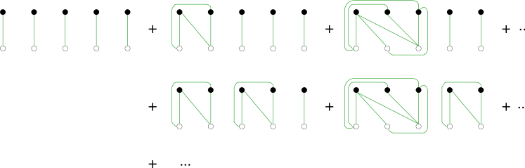
Figure 2: Generic graphical expansion of the planar part of the norms required in (47). For simplicity we have only depicted the case in which there is only one type of operator; open dots represent $\operatorname{Tr}(\hat{a}^{J})$ for fixed $J$ and black dots their hermitian conjugates. The lines represent planar multiple contractions of elementary oscillators. The graphs displayed here correspond to typical “large” terms in each of the expressions in the sum (47).

In trying to estimate how fast the norms (47) have to grow with $p$, one can see that even an exponential growth of the norms, say as $p!\,\gamma^{p}$ ($\gamma=\text{const}.$), does not lead to reasonable results. Namely, if we consider the expression $\sum_{p}{\cal P}(J,p)$, which has to be smaller than one, and assume exponential growth of norms, we would find that this sum behaves as

$$\sum_{p=0}^{\infty}{\cal P}(J,p) ={\cal C}^{2}\sum_{p=0}^{\infty}\frac{1}{p!}\left(\frac{\eta_{J}^{2}}{\lambda^{J}\gamma}\right)^{p}$$ (48)

$$=\exp\left(\frac{\eta_{J}^{2}}{\lambda^{J}\gamma}\right)\exp\left(-\frac{N}{\lambda}\operatorname{Tr}(a^{\dagger}a)\right)\,.$$

Hence we see that even when $N\rightarrow\infty$ (while keeping $\lambda$ arbitrary but smaller than one) the result will always be larger than 1 for some value of $J$. Since the calculation of the average number of particles requires a summation over all $J$, we conclude that we cannot assume this behaviour of the norms.

The situation which we face here is similar in spirit to the double-scaling BMN limit. As observed by Kristjansen et al. Kristjansen et al. (2002) and Constable et al. Constable et al. (2002), in the limit $N\sim J^{2}\rightarrow\infty$ correlators in general receive contributions from non-planar graphs of all genera. In this case, a new expansion parameter $J^{2}/N$ appears. In our case, $N\rightarrow\infty$ as well, but now the additional parameter which becomes large is the value of the $p_{i}$ for which the sum (35) has its maximum term. It would be interesting to understand whether our system also exhibits a double-scaling limit in which some ratio of powers of $p$ and $N$ is kept fixed.

In order to determine the correct values of the norms of the states, it is useful to write the norms in terms of correlators of a complex matrix model,

$$\big{\langle}0\big{|}\Big{[}\big{(}\hat{O}_{J_{1}}\big{)}^{p_{1}}\ldots\big{(}\hat{O}_{J_{n}}\big{)}^{p_{n}}\Big{]}\,\Big{[}\big{(}\hat{O}^{\dagger}_{J_{n}}\big{)}^{p_{n}}\ldots\big{(}\hat{O}^{\dagger}_{J_{1}}\big{)}^{p_{1}}\Big{]}\,\big{|}0\big{\rangle}=\\[4.30554pt] \int\!{\rm d}A{\rm d}\bar{A}\,\Big{[}\big{(}{O}_{J_{1}}\big{)}^{p_{1}}\ldots\big{(}{O}_{J_{n}}\big{)}^{p_{n}}\Big{]}\,\Big{[}\big{(}{O}^{\dagger}_{J_{n}}\big{)}^{p_{n}}\ldots\big{(}{O}^{\dagger}_{J_{1}}\big{)}^{p_{1}}\Big{]}\\[4.30554pt] \times\exp\Big{(}-\operatorname{Tr}(A^{\dagger}A)\Big{)}\,,$$ (49)

The measure used here is simply a separate integral over the real and imaginary parts of the complex matrix $A$, normalised to give unit result when all $p_{i}$ in the expression above are zero,

$$\int\!{\rm d}A{\rm d}\bar{A}=\pi^{-N}\prod_{a,b=1}^{N}{\rm d}(\operatorname{Re}A_{ab})\,\,\,{\rm d}(\operatorname{Im}A_{ab})\,.$$ (50)

This approach has been used by Kristjansen et al. Kristjansen et al. (2002); Beisert et al. (2003) in order to compute several special cases of (49) analytically. It is still an open problem to extend those exact results to the entire class of correlators, in particular to general situations for which $p_{i}>2$. Because we will need these very general correlators, we have decided to use an alternative approach, in which the integral is evaluated using Monte-Carlo methods. This provides us with a technically straightforward way to extract the norms for arbitrary operator insertions, even for very large $p_{i}$. Our results will, for this reason, of course be restricted to a fixed value for $N$, and computer resources put a practical limit on the maximum value that can be handled. Nevertheless, we will see that interesting results can be obtained this way.

Figure 3: Norms of states built from $J=2$ operators (lower two curves) and $J=4$ operators (upper two curves), as a function of the total number of operator insertions, for U(4). The dashed lines are the estimates based on the first two columns of graphs in figure 2. The continuous lines are the complete norms extracted from the Monte-Carlo analysis.

Before we discuss the results, let us present numerical evidence which illustrates the necessity of taking the full norms in (32) into account, i.e. all planar and non-planar contributions. We compare the results obtained by summing up a large class of planar diagrams in (47) with the numerical results obtained using the Monte-Carlo integration. For the U(4) case, the Monte-Carlo results are depicted in figure 3 and compared to the analytic answer obtained by restricting to the first two columns of graphs in figure 2; these columns contain graphs with an arbitrary number of connected four-blob elements. Clearly, the full norms deviate substantially from this estimate. Hence, in the remainder we will only employ the norms obtained by Monte-Carlo integration of (49). Note also from figure 2 that for large $p$, the deviation from the exact norm grows with increasing $J$ (and it also grows with increasing $N$), and does not improve as one might naively expect.

Figure 4: Plot of the summed probability, in $U(2)$, to find a state with zero or more $\hat{O}_{2}$ operators in $|c\rangle$, as a function of the maximum number of operator insertions $p^{\text{cutoff}}$ in (32). Equivalently, this is the total probability to find a singlet state in the coherent state. The two continuous lines correspond to two different values of the coupling constant. The dashed lines are the individual terms that make up the sum. Observe that these curves never reach one, which shows that there are still many states in the coherent state which are non-singlets.

With the correct norms of the multi-particle states at hand, one now obtains sensible results for the sums (34) and (35). An example in U(2) (which is rather trivial because there is in this case only one independent single-trace operator) is plotted in figure 4. Note once more that the numbers plotted here are much smaller than one. This is because the norm ${\cal C}$ which multiplies all of these results is the norm of the non-singlet coherent state, and the number of singlets in it is much smaller than the total number of states. Note, however, that since the norm of the coherent state appears in all probabilities as an overall (identical) factor, its absolute value is irrelevant when considering the ratios of emitted energies or ratios of numbers of particles. See appendix V.2 for a more explicit explanation.

Having resolved the computation of the exact norms of states, we can now finally compute the energy distribution in the outgoing state of a more interesting example. For practical reasons, we will restrict ourselves to the U(4) case, for which there are only two operators which create physical states (using only the creation operator for the lowest-lying spherical harmonics). These operators are $\operatorname{Tr}\big{(}(a^{\dagger})^{2}\big{)}$ and $\operatorname{Tr}\big{(}(a^{\dagger})^{4}\big{)}$. The proper linear combinations of these operators are

$$\hat{O}_{2}^{\dagger} =\operatorname{Tr}(a^{\dagger}a^{\dagger})\,,$$ (51)

$$\hat{O}_{4}^{\dagger} =\operatorname{Tr}(a^{\dagger}a^{\dagger}a^{\dagger}a^{\dagger})-\frac{2N^{2}+1}{N(N^{2}+2)}\operatorname{Tr}(a^{\dagger}a^{\dagger})\operatorname{Tr}(a^{\dagger}a^{\dagger})\,.$$

These lead to $\langle\hat{O}_{4}\,|\,\hat{O}_{2}\hat{O}_{2}\rangle=0$. Multi-particle states will generically not be orthogonal (see also footnote 9), but in our case this turns out to be far less important than the $1/N^{2}$ corrections to the norms. We will for simplicity use a classical configuration for which

$$\frac{\eta_{4}}{N}=\left(\frac{\eta_{2}}{N}\right)^{2}=\frac{\eta}{N}\,,$$ (52)

where the $\eta_{J}$ are defined in (46). Closer inspection of the coherent state of the sphaleron given in (22) shows that the expectation values of e.g. the $\operatorname{Tr}(F_{mn}F^{mn})$ and $\operatorname{Tr}(F_{mn}F^{mn}F_{rs}F^{rs})$ states are similarly related.

The energy radiated into $O_{2}$ and $O_{4}$ particles can be computed using formula (35), summed over a suitably large range of values for $p_{2}$ and $p_{4}$. In our particular case, this formula reduces to

$$E (J,p^{\text{cutoff}}_{2},p^{\text{cutoff}}_{4})=$$ (53)

$$\sum_{p_{2}=0}^{p_{2}^{\text{cutoff}}}\sum_{p_{4}=0}^{p_{4}^{\text{cutoff}}}\left|\frac{\eta_{2}^{2}}{\lambda^{2}}\right|^{p_{2}}\left|\frac{\eta_{4}^{2}}{\lambda^{4}}\right|^{p_{4}}\frac{Jp_{J}}{2^{p_{2}}4^{p_{4}}}$$

$$\times\frac{{\cal C}^{2}}{\langle 0|\,(\hat{O}_{2})^{p_{2}}(\hat{O}_{4})^{p_{4}}\,(\hat{O}_{4}^{\dagger})^{p_{4}}(\hat{O}_{2}^{\dagger})^{p_{2}}\,|0\rangle\,\langle c|c\rangle}\,.$$

and the maximum values of $p_{2}$ and $p_{4}$ which are included in the sum should be taken sufficiently large as to include at least the maximum term in the sum. This requirement is indeed met in our numerical approach.

\psfrag{10}{$\scriptstyle 10$}\psfrag{20}{$\scriptstyle 20$}\psfrag{40}{$\scriptstyle 40$}\psfrag{60}{$\scriptstyle 60$}\psfrag{-20}{$\scriptstyle~{}-20$}\psfrag{-40}{$\scriptstyle~{}-40$}\psfrag{-60}{$\scriptstyle~{}-60$}\psfrag{-80}{$\scriptstyle~{}-80$}\psfrag{0}{$\scriptstyle 0$}\psfrag{p2}{$\scriptstyle p_{2}^{\text{cutoff}}$}\psfrag{p4}{$\scriptstyle p_{4}^{\text{cutoff}}$}\includegraphics*[width=260.17464pt]{energies_math.eps}

\psfrag{10}{$\scriptstyle 10$}\psfrag{20}{$\scriptstyle 20$}\psfrag{40}{$\scriptstyle 40$}\psfrag{60}{$\scriptstyle 60$}\psfrag{-20}{$\scriptstyle~{}-20$}\psfrag{-40}{$\scriptstyle~{}-40$}\psfrag{-60}{$\scriptstyle~{}-60$}\psfrag{-80}{$\scriptstyle~{}-80$}\psfrag{0}{$\scriptstyle 0$}\psfrag{p2}{$\scriptstyle p_{2}^{\text{cutoff}}$}\psfrag{p4}{$\scriptstyle p_{4}^{\text{cutoff}}$}\includegraphics*[height=147.95424pt]{energies_overlay.eps}

Figure 5: Successive approximations to the logarithm of the total energy radiated in the $J=2$ particles (light, blue surface) and $J=4$ particles (dark, red surface). The $x$ and $y$ axes label the maximum value of $p_{2}$ and $p_{4}$ in the sum (53). The values asymptote to the full result in the upper left corner of the graph. The curves in the $x-z$ and $y-z$ plane are similar to the continuous lines in figure 4. While the present plot shows energies, qualitatively similar plots are obtained for the particle numbers.

We have computed the ratio of energies in the $J=2$ and $J=4$ particles using successive approximations of (53), for larger and larger $p^{\text{cutoff}}_{2}$ and $p_{4}^{\text{cutoff}}$,

$$\lim_{\begin{subarray}{c}\\ p^{\text{cutoff}}_{2}\rightarrow\infty\\[1.50694pt] p^{\text{cutoff}}_{4}\rightarrow\infty\end{subarray}}\frac{E(4,p^{\text{cutoff}}_{2},p^{\text{cutoff}}_{4})}{E(2,p^{\text{cutoff}}_{2},p^{\text{cutoff}}_{4})}=:R(\eta^{2}/\lambda^{2})$$ (54)

for a range of couplings. A typical example is plotted in figure 5. One clearly sees that the asymptotic value of the ratio (54), given by the exponent of the asymptotic height difference between the two surfaces, is smaller than one. We therefore conclude that our calculation predicts that higher-energy states in the decay product are suppressed with respect to the lower-energy ones. This is in qualitative agreement with alternative calculations of this decay process Lambert et al. (2003).

It would be very interesting to extend our analysis to higher-rank gauge groups, perhaps by obtaining an analytic expression for the norms of the states. For $N>4$, there are more than two gauge singlet states, and it becomes possible to determine the suppression factor as a function of the energy in more detail. We leave this for future investigations.

IV Discussion and open issues

We have presented the formalism to analyse the decay of unstable D-branes in the $\text{AdS}_{5}\times S^{5}$ background by considering the dual gauge theory. Our results show qualitative agreement with previous work on D-particle decay, and our paper provides the basis for further study of non-perturbative dynamical features of the correspondence. Let us conclude by describing a number of open issues and possible extensions of our work.

One obvious way to improve on our results would be to determine analytical expressions for the norms required in section III.3 (using the construction of states in terms of group characters Balasubramanian et al. (2002); Corley et al. (2002); Kristjansen et al. (2002)). This would allow one to extend the results obtained there to large values of $N$. We expect that already for the U(6) model it should be possible to get evidence that the observed suppression of the decay products with their mass is actually exponential. It would be interesting to see whether this suppression is strong enough to compete with the Hagedorn growth of the multiplicity of states at high mass levels. Obtaining these results should enable one to check whether the total energy emitted in the decay product is finite or not.

The flat space string calculation of Lambert et al. (2003) and the matrix model calculation of McGreevy and Verlinde (2003) both obtained an infinite total energy for the final decay product. One might think that the reason for such behavior is that there is non-trivial back-reaction of the radiated closed strings on the boundary state, which has not been taken into account. However, it was argued in Klebanov et al. (2003); Sen (2004, 2004) that the time dependent boundary state of Sen (2002) already contains the full information about the closed string sector into which it is going to decay. Instead, the reason for the divergences observed in Lambert et al. (2003); McGreevy and Verlinde (2003) has been attributed to the fact that the coherent state of the unstable brane has an infinite spread in energy (in the fermionic description it corresponds to a sharply localised fermion in position space).

We believe that, whatever the reason for the observed divergence, the emitted energy calculated from our coherent state should be finite. In our setup there is no issue of backreaction, since there is no separation between the source and the “remainder” in our system. For the construction of the coherent state we have used a solution of the full, non-linear Yang-Mills equations of motion. Also, as one can check, the coherent state thus constructed has finite spread both in momentum and position space, hence avoiding the aforementioned problem.

To make a link of our work to the comments of Sen (2004, 2004) and as a comparison to the matrix model, let us note that the classical tachyon evolution is governed by the reduced Yang-Mills action (8) (or, to be more precise, to a similar reduction based on more general gauge group embeddings of the type (14)). One might hope that this action is dual to the open string field theory on decaying D-particles in the bulk of AdS. However, this requires further analysis.

As we have explained, due to the non-perturbative nature of the initial sphaleron configuration, the computation of the decay product requires information from a regime in which both $N\rightarrow\infty$ as well as the number of particles  $p\rightarrow\infty$. Understanding this double limit might circumvent the need to calculate the state norms exactly when calculating the energy distribution in the final state. Finally, it would be interesting to understand how quantum corrections can be incorporated into our formalism, in order to see how much they influence the qualitative characteristics of the decay product.

V Appendix

V.1 $S^{2}$ operator–state correspondence

We will here consider the operator–state correspondence in the context of a simple $S^{2}\times\mathbb{R}$ example. Using the procedure outlined in the main text, let us construct all states corresponding to set of operators

$$\hat{O}_{1} :=\operatorname{Tr}\Big{(}\partial_{(\mu}\chi\partial_{\nu)}\chi\Big{)}-\frac{1}{d}g_{\mu\nu}\operatorname{Tr}\Big{(}\partial_{\rho}\chi\partial^{\rho}\chi\Big{)}\,,$$ (55)

$$\hat{O}_{2} :=\operatorname{Tr}\Big{(}\partial_{\rho}\chi\partial^{\rho}\chi\Big{)}\,,$$

$$\hat{O}_{3} :=\operatorname{Tr}\Big{(}\chi\partial_{\mu}\partial_{\nu}\chi\Big{)}\,.$$

Using the counting of states introduced by Sundborg Sundborg (2000) and Polyakov Polyakov (2002) (see also Aharony et al. Aharony et al. (2003)) we see that the total number of states created by these operators is

$$\partial_{\mu}\chi\partial_{\nu}\chi :\quad\frac{3\cdot 4}{2}=6\quad\text{states}\,,$$ (56)

$$\chi\partial_{\mu}\partial_{\nu}\chi :\quad\frac{3\cdot 4}{2}-1=5\quad\text{states}\,,$$

giving in total $11$ states. This means that the operators (55) also create $11$ states, since they are all possible operators one can build out of building blocks (56). Let us first count the number of states created by the operator $\hat{O}_{2}$. The operator has dimension $\Delta=3$, hence we can decompose it onto the various states as follows

$$\lim_{\tau\rightarrow-\infty}\int_{S^{2}}e^{-3\tau}\sum_{l^{\prime\prime},m^{\prime\prime}}Y_{l^{\prime\prime}m^{\prime\prime}}\,\partial_{\rho}\Big{(}\sum_{l,m}e^{\frac{1}{2}(2l+1)\tau}Y^{*}_{lm}a^{\dagger}_{lm}\Big{)}\partial^{\rho}\Big{(}\sum_{l^{\prime},m^{\prime}}e^{\frac{1}{2}(2l^{\prime}+1)\tau}Y^{*}_{l^{\prime}m^{\prime}}a^{\dagger}_{l^{\prime}m^{\prime}}\Big{)}|0\rangle\,.$$ (57)

Note that while the spherical harmonics which figure in the expansion of the field $\chi$ are on-shell, the spherical harmonics $Y_{l^{\prime\prime}m^{\prime\prime}}$ onto which we project need not be on-shell. Clearly the options for $(l,l^{\prime})$ in (57) are $(2,0)$, (i.e. $(0,2)$) and $(1,1)$. The explicit expressions before integration are (${\cal N}_{i,j}$ are normalisation constants)

$$\partial_{\mu}\chi\partial^{\mu}\chi\Big{|}_{(l,l^{\prime})=(0,2)}|0\rangle =\frac{5}{8\sqrt{\pi}}\sum_{m^{\prime}}Y^{*}_{2m^{\prime}}\,a^{\dagger}_{00}a^{\dagger}_{2m^{\prime}}|0\rangle\,,$$ (58)

$$\partial_{\mu}\chi\partial^{\mu}\chi\Big{|}_{(l,l^{\prime})=(1,1)}|0\rangle =\frac{5}{4\sqrt{\pi}}\Bigg{[}\begin{aligned} &(a^{\dagger}_{1,-1})^{2}{\cal N}_{1,-1}^{2}\Big{(}\frac{5}{4}\sin^{2}\theta\Big{)}e^{2i\phi}+(a^{\dagger}_{1,1})^{2}{\cal N}_{1,1}^{2}\Big{(}\frac{5}{4}\sin^{2}\theta\Big{)}e^{-2i\phi}\\ +&(a^{\dagger}_{1,0})^{2}{\cal N}_{1,0}^{2}\Big{(}\frac{9}{4}\cos^{2}\theta\Big{)}\\ +&\,a^{\dagger}_{1,1}a^{\dagger}_{1,-1}{\cal N}_{1,1}{\cal N}_{1,-1}\Big{(}-4-\frac{5}{2}\sin^{2}\theta\Big{)}\\ +&\,a^{\dagger}_{1,-1}a^{\dagger}_{1,0}{\cal N}_{1,-1}{\cal N}_{1,0}\Big{(}\frac{5}{2}\sin\theta\cos\theta\Big{)}e^{i\phi}\\ +&\,a^{\dagger}_{1,1}a^{\dagger}_{1,0}{\cal N}_{1,1}{\cal N}_{1,0}\Big{(}-4\sin\theta\cos\theta\Big{)}e^{-i\phi}\Bigg{]}|0\rangle\,.\end{aligned}$$

We see that projection onto the $Y_{l^{\prime\prime}m^{\prime\prime}}$ modes with $l^{\prime\prime}=2$ would give five non-zero projections (the $a^{\dagger}_{1,1}a^{\dagger}_{1,-1}$ and $(a^{\dagger}_{0})^{2}$ come together), which is too many. The correct procedure is to use the lowest harmonic $l^{\prime\prime}=0$, in which case only one state (the second and third lines in (58)) is selected. If one repeats similar exercises with the operators $\hat{O}_{1}$ and $\hat{O}_{3}$, one obtains states that are not orthogonal to states obtained from $\hat{O}_{2}$ unless one uses the appropriate lowest lying tensor spherical harmonic. To see this we need to use the tensor harmonics on $S^{2}$. There are four types of lowest-lying 2-tensor spherical harmonics:

$$\eta_{ab}^{(lm)} =Y^{(lm)}g_{ab}\,, \quad l\geq 0\,,$$ (59)

$$\psi_{ab}^{(lm)} =Y^{(lm)}_{;ab}+\tfrac{1}{2}l(l+1)\,, \quad l\geq 2\,,$$ (60)

$$\chi_{ab}^{(lm)} =Y^{(lm)}\epsilon_{ab}\,, \quad l\geq 0\,,$$ (61)

$$\phi_{ab}^{(lm)} =\tfrac{1}{2}\big{(}\phi_{a;b}^{(lm)}+\phi_{b;a}^{(lm)}\big{)}\,, \quad l\geq 2\,,$$ (62)

where $\phi_{a}^{(lm)}$ is a vector spherical harmonic, given by $\phi_{a}^{(lm)}=\epsilon_{a}{}^{b}Y^{(lm)}_{,b}$. The $\eta$ mode is a pure trace so it does not contribute when contracted with $\hat{O}_{1}$ or $\hat{O}_{3}$ and the equations of motion for $\chi$ are used. Furthermore, the $\chi$ mode is anti-symmetric, so it also leads to a zero. Thus we find, by explicitly contracting $\psi$ and $\phi$ with the two operators, multiplying with $e^{-3\tau}$ and taking the $\tau\rightarrow-\infty$ limit, and finally integrating over $S^{2}$, that

$$\int_{S^{2}}\psi_{ab}^{(l=2,m=-2)}\hat{O}_{1}^{ab}\,{\rm d}\Omega \sim\big{(}a^{\dagger}_{1,1}\big{)}^{2}|0\rangle\,,$$ (63)

$$\int_{S^{2}}\phi_{ab}^{(l=2,m=-2)}\hat{O}_{1}^{ab}\,{\rm d}\Omega =0\,,$$

$$\int_{S^{2}}\psi_{ab}^{(l=2,m=-2)}\hat{O}_{3}^{ab}\,{\rm d}\Omega \sim a^{\dagger}_{2,2}a^{\dagger}_{0,0}|0\rangle\,,$$

$$\int_{S^{2}}\psi_{ab}^{(l=2,m=-2)}\hat{O}_{3}^{ab}\,{\rm d}\Omega =0\,,$$

and with similar expressions for the other $4$ labels $(2,1)$, $(2,0)$, $(2,-1)$ and $(2,-2)$. Note however, that all these expressions involve different bilinears of operators $a^{\dagger}$ and hence are automatically orthogonal.

In summary, we thus find that the operators $\hat{O}_{1}$ and $\hat{O}_{3}$ create $5$ states each, while operator $\hat{O}_{2}$ corresponds to a single state, altogether giving a total of $11$ states as required by (56).

V.2 Singlet projections

We will here use a simple example to show how the smallness of the expectation values plotted in e.g. figure 4 can be understood. As mentioned in the main text, the crucial reason is that the coherent state used to make these plots was the state $|c\rangle$ (rather than the state (24)), and this state contains both singlet and non-singlet states. We have argued that the suppression in figure 4 is determined by the number of singlets versus the number of non-singlet states in $|c\rangle$. To illustrate this, we will here use the $J=2$ operator in U(2), for a non-abelian scalar. There are four elementary operators $\hat{a}^{\dagger},\ldots\hat{d}^{\dagger}$,

$$\hat{A}^{\dagger}=\begin{pmatrix}\hat{a}^{\dagger}&\hat{b}^{\dagger}\\ \hat{c}^{\dagger}&\hat{d}^{\dagger}\end{pmatrix}\,.$$ (64)

and each of these satisfies a canonical commutation relation with its conjugate. For the classical field, let us take the simple example of

$$A_{\text{class.}}=\begin{pmatrix}\eta&0\\ 0&0\end{pmatrix}\,.$$ (65)

This implies that the coherent state is given by

$$|c\rangle={\cal C}\,\exp\Big{(}\frac{1}{g^{2}}\operatorname{Tr}\big{(}A_{\text{class.}}\hat{A}^{\dagger}\big{)}\Big{)}|0\rangle={\cal C}\,\exp\Big{(}\frac{1}{g^{2}}\eta\hat{a}^{\dagger}\Big{)}|0\rangle\,.$$ (66)

The correct normalisation constant is thus

$${\cal C}^{2}=\exp\big{(}-\frac{\eta^{2}}{g^{2}}\big{)}\,.$$ (67)

We always compute projections of the coherent state onto gauge-singlet states. Let us consider the $p=1$ case,

$$\frac{\Big{|}\big{\langle}0\big{|}\operatorname{Tr}(\hat{A}^{2})\big{|}c\big{\rangle}\Big{|}^{2}}{{\big{<}0\big{|}\operatorname{Tr}(\hat{A}^{2})\,\operatorname{Tr}((\hat{A}^{\dagger})^{2})\big{|}0\big{\rangle}\,\big{\langle}c\big{|}c\big{\rangle}}}\,.$$ (68)

The norm in the denominator equals $2N^{2}g^{4}=8g^{4}$. This gives, if one adds the trivial $p=0$ term,

$${\cal P}(J=2)={\cal C}^{2}\Big{(}1+\frac{\eta^{4}}{8\,g^{4}}+\ldots\Big{)}=\frac{\Big{(}1+\frac{\eta^{4}}{8\,g^{4}}+\ldots\Big{)}}{\Big{(}1+\frac{\eta^{2}}{g^{2}}+\frac{\eta^{4}}{2\,g^{4}}+\ldots\Big{)}}\,.$$ (69)

Here we have expanded ${\cal C}^{2}$ in the second step. The fact that ${\cal P}(J=2)$ comes out smaller than $1$ has two reasons. Firstly, the odd powers of $\eta^{2}/g^{2}$ are manifestly absent from the numerator, since they correspond to the states with odd powers of the operator $\hat{a}$ and are hence manifestly non-singlets. Secondly, the coefficient of $\eta^{4}/g^{4}$ in the numerator is only $1/8$, as compared to the $1/2$ in the denominator. This is because out of all quadratic operators that involve the operator $\hat{a}$ in some combination with the operators $\hat{a}\ldots\hat{d}$, only one is a trace operator. We are focusing on the operators that necessarily involve $\hat{a}$, since all other operators are absent in the coherent state. In the sector which contains $\hat{a}^{2}$, $\hat{b}\hat{c}$ and $\hat{d}^{2}$, there are three of those,

$$\hat{O}_{1}=\hat{a}^{2}+2\hat{b}\hat{c}+\hat{d}^{2}\,,\quad\hat{O}_{2}=\hat{a}^{2}-2\hat{b}\hat{c}+\hat{d}^{2}\,,\quad\hat{O}_{3}=\hat{a}^{2}-\hat{d}^{2}\,.$$ (70)

As given here, these are orthogonal. However, only $\hat{O}_{1}$ is a single-trace operator.

If we also compute the projection of the coherent state onto $\hat{O}_{2}$ and $\hat{O}_{3}$, and add these probabilities to the one found for $\hat{O}_{1}$, we get

$${\cal P}(J=2)={\cal C}^{2}\Big{(}1+\frac{\eta^{4}}{g^{4}}\Big{[}\frac{1}{8}+\frac{1}{8}+\frac{1}{4}\Big{]}+\ldots\Big{)}\,.$$ (71)

Now the $1/2$ precisely matches the $1/2$ in ${\cal C}^{2}$.

Note that this issue becomes more and more serious as we go up in the number of operator insertions. The very small numbers as presented in section III.3 thus arise because these only count multi-particle singlet states, as opposed to generic multi-particle states.

V.3 Geometrical expressions

In this section we collect some intermediate results of the calculations and some useful formulae that were used in the main text. The coordinates which we use on $\mathbb{R}\times S^{3}$ are related to Cartesian coordinates via

$$z_{1} =x^{0}+ix^{1}$$ (72)

$$r\cos\left(\frac{\theta}{2}\right) =\left(\cos\left(\frac{\phi+\psi}{2}\right)+i\sin\left(\frac{\phi+\psi}{2}\right)\right)\,,$$

$$z_{2} =x^{3}+ix^{4}$$

$$r\cos\left(\frac{\theta}{2}\right) =\left(\cos\left(\frac{\phi-\psi}{2}\right)+i\sin\left(\frac{\phi+\psi}{2}\right)\right)\,,$$

after which we perform a conformal rescaling to obtain the metric

$${\rm d}s^{2}=-{\rm d}t^{2}+\frac{R^{2}}{4}\Big{(}{\rm d}\theta^{2}+{\rm d}\psi^{2}+{\rm d}\phi^{2}+2\,\cos\theta\,{\rm d}\psi{\rm d}\phi\Big{)}\,.$$ (73)

The coordinate ranges are given by $\theta\in[0,\pi\rangle$, $\phi\in[0,2\pi\rangle$ and $\psi\in[0,4\pi\rangle$. The volume of the $S^{3}$ part is thus computed to be $\operatorname{vol}(S^{3})=2\pi^{2}R^{3}$. The inverse metric is

$$g^{\theta\theta}=\frac{4}{R^{2}}\,\quad g^{\phi\phi}=g^{\psi\psi}=\frac{4}{R^{2}\,\sin^{2}(\theta)}\,\quad g^{\psi\phi}=-\frac{4\cos\theta}{R^{2}\,\sin^{2}\theta}$$ (74)

and the connection

$$\Gamma^{\theta}_{\phi\psi} =\frac{1}{2}\sin\theta\,,$$ (75)

$$\Gamma^{\phi}_{\phi\theta} =\Gamma^{\psi}_{\psi\theta}=\frac{\cos\theta}{2\sin\theta}\,,$$

$$\Gamma^{\phi}_{\psi\theta} =\Gamma^{\psi}_{\phi\theta}=-\frac{1}{2\sin\theta}$$

The gauge potential (5) in coordinates $(t,\theta,\phi,\psi)$ reads

$$A_{t} =0\,,$$ (76)

$$A_{\theta} =\frac{i}{2}f(t)(\cos\phi\,\sigma_{2}-\sin\phi\,\sigma_{3})\,,$$

$$A_{\phi} =\frac{i}{2}f(t)\sigma_{1}\,,$$

$$A_{\psi} =\frac{i}{2}f(t)(\cos\theta\,\sigma_{1}+\sin\theta\sin\phi\,\sigma_{2}+\sin\theta\cos\phi\,\sigma_{3})\,.$$

The field strength is defined by

$$F_{\mu\nu}=\partial_{\mu}A_{\nu}-\partial_{\nu}A_{\mu}-[A_{\mu},A_{\nu}]\,,$$ (77)

and the corresponding gauge transformations are

$$A_{\mu}\rightarrow\Lambda A_{\mu}\Lambda^{\dagger}-\Lambda\partial_{\mu}\Lambda^{\dagger}\,.$$ (78)

For the sphaleron configuration (5), the field strenghts are given by

$$F_{\theta\phi} =B(\sin\phi\sigma_{2}+\cos\phi\sigma_{3})\,,$$ (79)

$$F_{\theta\psi} =B(-\sin\theta\sigma_{1}+\sin\phi\cos\theta\sigma_{2}+\cos\theta\cos\phi\sigma_{3})\,,$$

$$F_{\phi\psi} =B(\sin\theta\cos\phi\sigma_{2}-\sin\theta\sin\phi\sigma_{3})\,$$

$$F_{0\theta} =\frac{\dot{f}}{f}A_{\theta}\,\quad F_{0\psi}=\frac{\dot{f}}{f}A_{\psi}\,\quad F_{0\phi}=\frac{\dot{f}}{f}A_{\phi}\,,$$

$$B \equiv\frac{if}{2}(1-f)\,.$$

The lowest-order vector spherical harmonics are related to the canonically normalised left-invariant one-forms as

$$Y_{\tfrac{1}{2}(0,0)\tfrac{1}{2}} =\frac{i}{2}\frac{1}{\sqrt{\operatorname{vol}(S^{3})}}\Sigma^{3}\,, \Sigma^{1} =\sqrt{2\operatorname{vol}(S^{3})}i\Big{(}Y_{\tfrac{1}{2}(1,0)\tfrac{1}{2}}+Y_{\tfrac{1}{2}(-1,0)\tfrac{1}{2}}\Big{)}\,,$$ (80)

$$Y_{\tfrac{1}{2}(-1,0)\tfrac{1}{2}} =\frac{1}{2\sqrt{2}}\frac{1}{\sqrt{\operatorname{vol}(S^{3})}}\Big{(}-\Sigma^{2}-i\Sigma^{1}\Big{)}\,,\quad \Sigma^{1} =\sqrt{2\operatorname{vol}(S^{3})}i\Big{(}Y_{\tfrac{1}{2}(1,0)\tfrac{1}{2}}+Y_{\tfrac{1}{2}(-1,0)\tfrac{1}{2}}\Big{)}\,,$$

$$Y_{\tfrac{1}{2}(1,0)\tfrac{1}{2}} =\frac{1}{2\sqrt{2}}\frac{1}{\sqrt{\operatorname{vol}(S^{3})}}\Big{(}+\Sigma^{2}-i\Sigma^{1}\Big{)}\,,\quad \Sigma^{3} =-2i\sqrt{\operatorname{vol}(S^{3})}Y_{\tfrac{1}{2}(0,0)\tfrac{1}{2}}\,.$$

Here the left-invariant one-forms are given by

$$\Sigma^{1} =\hphantom{-}\cos\psi\,{\rm d}\theta+\sin\psi\sin\theta\,{\rm d}\phi\,,$$ (81)

$$\Sigma^{2} =-\sin\psi\,{\rm d}\theta+\cos\psi\sin\theta\,{\rm d}\phi\,,$$

$$\Sigma^{3} =\hphantom{-}\cos\theta\,{\rm d}\phi+{\rm d}\psi\,,$$

For the explanation of indices, see formula (19).

References

- Sen (2002) A. Sen, “Rolling tachyon”, JHEP 04 (2002) 048, hep-th/0203211.
- McGreevy and Verlinde (2003) J. McGreevy and H. Verlinde, “Strings from tachyons: the matrix reloaded”, JHEP 12 (2003) 054, hep-th/0304224.
- Harvey et al. (2000) J. A. Harvey, P. Horava, and P. Kraus, “D-sphalerons and the topology of string configuration space”, JHEP 03 (2000) 021, hep-th/0001143.
- Manton (1983) N. S. Manton, “Topology in the Weinberg-Salam theory”, Phys. Rev. D28 (1983) 2019.
- Drukker et al. (2000) N. Drukker, D. J. Gross, and N. Itzhaki, “Sphalerons, merons and unstable branes in AdS”, Phys. Rev. D62 (2000) 086007, hep-th/0004131.
- Gubser et al. (1998) S. S. Gubser, I. R. Klebanov, and A. A. Tseytlin, “Coupling constant dependence in the thermodynamics of supersymmetric Yang-Mills theory”, Nucl. Phys. B534 (1998) 202, hep-th/9805156.
- Zadrozny (1992) J. Zadrozny, “Sphaleron decay products: A coherent state analysis”, Phys. Lett. B284 (1992) 88–93.
- Hellmund and Kripfganz (1992) M. Hellmund and J. Kripfganz, “The decay of the sphalerons”, Nucl. Phys. B373 (1992) 749–760.
- Lambert et al. (2003) N. Lambert, H. Liu, and J. Maldacena, “Closed strings from decaying D-branes”, hep-th/0303139.
- Klinkhamer and Manton (1984) F. R. Klinkhamer and N. S. Manton, “A saddle point solution in the Weinberg-Salam theory”, Phys. Rev. D30 (1984) 2212.
- Gibbons and Steif (1994) G. W. Gibbons and A. R. Steif, “Yang-Mills cosmologies and collapsing gravitational sphalerons”, Phys. Lett. B320 (1994) 245–252, hep-th/9311098.
- Volkov (1996a) M. S. Volkov, “Sphaleron on ”, Helv. Phys. Acta 69 (1996)a 289–292, hep-th/9609200.
- Volkov (1996b) M. S. Volkov, “Computation of the winding number diffusion rate due to the cosmological sphaleron”, Phys. Rev. D54 (1996)b 5014–5030, hep-th/9604054.
- Cahill (1974) K. Cahill, “Extended particles and solitons”, Phys. Lett. B53 (1974) 174.
- Pottinger (1978) D. E. L. Pottinger, “Creation and annihilation operators for Nielsen-Olesen vortices in the coherent state approximation”, Phys. Lett. B78 (1978) 476.
- Hamada and Horata (2003) K. Hamada and S. Horata, “Conformal algebra and physical states in non-critical 3-brane on ”, Prog. Theor. Phys. 110 (2003) 1169–1210, hep-th/0307008.
- Klauder and Skagerstam (1985) J. Klauder and B. Skagerstam, “Coherent states; applications in physics and mathematical physics”, World Scientific, 1985.
- Sundborg (2000) B. Sundborg, “The Hagedorn transition, deconfinement and SYM theory”, Nucl. Phys. B573 (2000) 349–363, hep-th/9908001.
- Fubini et al. (1973) S. Fubini, A. J. Hanson, and R. Jackiw, “New approach to field theory”, Phys. Rev. D7 (1973) 1732–1760.
- Brittin and Sakakura (1980a) W. E. Brittin and A. Y. Sakakura, “Number operators for composite particles in nonrelativistic many body theory”, J. Math. Phys. 21 (1980)a 2164–2169.
- Brittin and Sakakura (1980b) W. E. Brittin and A. Y. Sakakura, “Composite particles in nonrelativistic many-body theory: Foundations and statistical mechanics”, Phys. Rev. A21 (1980)b 2050–2063.
- Das and Trivedi (1998) S. R. Das and S. P. Trivedi, “Three brane action and the correspondence between Yang-Mills theory and anti-de-Sitter space”, Phys. Lett. B445 (1998) 142–149, hep-th/9804149.
- Kim et al. (1985) H. J. Kim, L. J. Romans, and P. van Nieuwenhuizen, “The mass spectrum of chiral , supergravity on ”, Phys. Rev. D32 (1985) 389.
- Sen (2004) A. Sen, “Rolling tachyon boundary state, conserved charges and two dimensional string theory”, JHEP 05 (2004) 076, hep-th/0402157.
- Gutperle and Strominger (2003) M. Gutperle and A. Strominger, “Timelike boundary Liouville theory”, Phys. Rev. D67 (2003) 126002, hep-th/0301038.
- Kristjansen et al. (2002) C. Kristjansen, J. Plefka, G. W. Semenoff, and M. Staudacher, “A new double-scaling limit of super Yang-Mills theory and pp-wave strings”, Nucl. Phys. B643 (2002) 3–30, hep-th/0205033.
- Constable et al. (2002) N. R. Constable, D. Z. Freedman, M. Headrick, and S. Minwalla, “Operator mixing and the BMN correspondence”, JHEP 10 (2002) 068, hep-th/0209002.
- Beisert et al. (2003) N. Beisert, C. Kristjansen, J. Plefka, G. W. Semenoff, and M. Staudacher, “BMN correlators and operator mixing in super Yang-Mills theory”, Nucl. Phys. B650 (2003) 125–161, hep-th/0208178.
- Balasubramanian et al. (2002) V. Balasubramanian, M. Berkooz, A. Naqvi, and M. J. Strassler, “Giant gravitons in conformal field theory”, JHEP 04 (2002) 034, hep-th/0107119.
- Corley et al. (2002) S. Corley, A. Jevicki, and S. Ramgoolam, “Exact correlators of giant gravitons from dual SYM theory”, Adv. Theor. Math. Phys. 5 (2002) 809–839, hep-th/0111222.
- Klebanov et al. (2003) I. R. Klebanov, J. Maldacena, and N. Seiberg, “D-brane decay in two-dimensional string theory”, JHEP 07 (2003) 045, hep-th/0305159.
- Sen (2004) A. Sen, “Open-closed duality: Lessons from matrix model”, Mod. Phys. Lett. A19 (2004) 841–854, hep-th/0308068.
- Polyakov (2002) A. M. Polyakov, “Gauge fields and space-time”, Int. J. Mod. Phys. A17S1 (2002) 119–136, hep-th/0110196.
- Aharony et al. (2003) O. Aharony, J. Marsano, S. Minwalla, K. Papadodimas, and M. Van Raamsdonk, “The Hagedorn/deconfinement phase transition in weakly coupled large- gauge theories”, hep-th/0310285.