Unstable D-branes and String Cosmology

Abstract

Cosmological implication of rolling tachyons is reported in the context of effective field theory. With a brief review of rolling tachyons in both flat and curved spacetimes, we study the string cosmological model with both tachyon and dilaton. In the string frame, flat space solutions of both initial-stage and late-time are obtained in closed form. In the Einstein frame, every expanding solution is decelerating. When a Born-Infeld U(1) gauge field is coupled, enhancement of e-folding of scale factor is also discussed by numerical analysis.

I Introduction

Rolling tachyons have been proposed for the description of the homogeneous decay of unstable D-brane in terms of both boundary conformal field theory Sen:2002nu and effective field theory Sen:2002an . The role of rolling tachyons has been tested in cosmology Gibbons:2002md , i.e., various topics include inflation, dark matter, cosmological perturbation, and reheating Fairbairn:2002yp ; Felder:2002sv ; Mehen:2002xr ; Kim:2002zr ; Gibbons:2003gb ; Kim:2003qz ; Mazumdar:2001mm . Though the tachyon driven cosmology is also a subject of string theory, the basic language is effective field theory of the tachyon and graviton. In this note, we will study the effects of linear dilaton from the bulk and Born-Infeld type electromagnetic fields living on the brane in addition to the two compulsory fields since the dilaton and Born-Infeld type gauge fields are natural in string cosmology. Another intriguing description of the rolling tachyons in (1+1)-dimensional string theory is the $c=1$ matrix model McGreevy:2003kb , however the cosmology based on this language seems not realistic yet Karczmarek:2003pv .

The rest of this note is organized as follows. In section 2 and 3, we review the rolling tachyons in both flat and curved spacetime. In section 4, we consider the cosmology driven by rolling tachyons in the context of string cosmology with dilaton. In section 5, we find all possible rolling tachyon solutions in the presence of Born-Infeld type electromagnetic fields. In section 6, cosmological implication of such electromagnetic fields is studied in relation with inflation. Section 7 is devoted to concluding remarks.

II Rolling Tachyons in Effective Theory

Let us begin this section with recapitulating the rolling tachyon solution in the context of effective field theory Sen:2002an . Instability of an unstable D$p$-brane is described by the effective action of tachyon $T$;

$$S = -{\cal T}_{p}\int d^{p+1}x\,V(T)\sqrt{-\det(\eta_{\mu\nu}+\partial_{\mu}T\partial_{\nu}T)}$$ (1)

$$= -{\cal T}_{p}\int d^{p+1}x\,V(T)\sqrt{1+\partial_{\mu}T\partial^{\mu}T}\,,$$

where ${\cal T}_{p}$ is tension of the D$p$-brane.

Since tachyon potential measures variable tension of the unstable D-brane, it should be a runaway potential connecting $V(T=0)=1$ and $V(T=\infty)=0$. For the case of superstring, ${\rm Z}_{2}$-symmetry around its maximum at the origin is assumed, $V(T)=V(-T)$. Various forms of it have been proposed, e.g., $V(T)\sim e^{-T^{2}}$ with different derivative terms from boundary string field theory Gerasimov:2000zp or $V(T)\sim e^{-|T|}$ for large $|T|$ in Ref. Sen:2002an . In this paper, we employ the form Buchel:2002tj ; Kim:2003he ; Kim:2003qz ; Leblond:2003db

$$V(T)=\frac{1}{\cosh\left(\frac{T}{R}\right)}$$ (2)

which connects the small and the large $T$ behaviors smoothly. Here, $R$ is $\sqrt{2}$ for the non-BPS D-brane in the superstring and 2 for the bosonic string.

Most of the physics of tachyon condensation is irrelevant to the detailed form of the potential once it satisfies the runaway property and the boundary values. So do the cosmological issues. On the other hand, there are also the noteworthy features with the 1/cosh potential (2) in the effective field theory: (i) Exact solutions are obtained for rolling tachyon Kim:2003he ; Kim:2003ma and tachyon kink solutions on unstable D$p$ with a coupling of abelian gauge field for arbitrary $p$ Lambert:2003zr ; Kim:2003in ; Kim:2003ma ; Kim:2003uc . (ii) This form of the potential has been derived in open string theory by taking into account the fluctuations around $\frac{1}{2}$S-brane configuration with the higher derivatives neglected, i.e., $\partial^{2}T=\partial^{3}T=\cdots=0$ Kutasov:2003er ; Okuyama:2003wm . In addition, the obtained classical solutions of the effective field theory (1) can be directly translated to those of the linearized tachyon equation in open string theory described by BCFT, i.e., an effective tachyon field $T(x)$ at on-shell and a BCFT tachyon profile $\tau(x)$ has a one-to-one correspondence Kutasov:2003er

$$\frac{\tau(x)}{R}=\sinh\left(\frac{T(x)}{R}\right).$$ (3)

(iii) Among the tachyon soliton solutions in the effective theory, various tachyon array solutions of codimension one have been found, namely, those formed by pure tachyon kink-antikink Sen:1998tt ; Sen:1998ex ; Lambert:2003zr ; Kim:2003in , tachyon kink-antikink coupled to the electromagnetic field Kim:2003in ; Sen:2003bc ; Kim:2003ma , and tachyon tube-antitube Kim:2003uc ; Kim:2004xk . An interesting property of all these solutions is that the periodicity of the array is independent of any integration constant of the equation of motion only under Eq. (2) Kim:2004xk . This periodic property of the array configurations in the effective field theory is desirable if we wish to identify the array solution as a pair of D$(p-1)\bar{{\rm D}}(p-1)$ obtained from an unstable D$p$-brane wrapped on a cycle in the context of string theory Sen:1998ex ; Horava:1998jy ; Sen:2003bc .

Let us discuss the rolling tachyon solutions in what follows. Suppose a homogeneous configuration $T(t)$. Then the Lagrangian density is given by

$${\cal L}=-{\cal T}_{p}V(T)\sqrt{1-\dot{T}^{2}},$$ (4)

where the overdot $\dot{}$ denotes derivative of time. The conjugate momentum density is

$$\Pi\equiv\frac{\partial{\cal L}}{\partial\dot{T}}=\frac{{\cal T}_{p}V(T)\dot{T}}{\sqrt{1-\dot{T}^{2}}},$$ (5)

and Hamiltonian density is given by

$${\cal H}=\sqrt{\Pi^{2}+({\cal T}_{p}V)^{2}}.$$ (6)

Conservation of the Hamiltonian density $d{\cal H}/dt=\{{\cal H},{\cal H}\}_{\mathrm{P.B.}}=0$ leads to constant energy density

$${\cal H}=\rho=\frac{{\cal T}_{p}V}{\sqrt{1-\dot{T}^{2}}}$$ (7)

which results in an integral equation

$$\int\frac{dT}{\sqrt{1-({\cal T}_{p}V)^{2}/{\rho}^{2}}}=t+\mathrm{constant}.$$ (8)

For the specific form of tachyon potential (2), the integral equation (8) yields Kim:2003he

$$\sinh\frac{T(t)}{R}=a_{+}e^{t/R}-a_{-}e^{-t/R},$$ (9)

where $a_{\pm}$ are related to the initial conditions as

$$a_{\pm}=\frac{1}{2}\left[\dot{T}_{i}\cosh(T_{i}/R)\pm\sinh(T_{i}/R)\right],$$

$$T_{i}\equiv T(0)~{}\mbox{and}~{}\dot{T}_{i}\equiv\dot{T}(0).$$ (10)

Due to time translation invariance and reflection symmetries ($T\leftrightarrow-T$ and $t\leftrightarrow-t$), the rolling tachyon solution (9) is rewritten as a one-parameter family solution of ${\cal E}$ in a simpler form

$$\left\{\begin{array}[]{lccl}\sinh\left(T_{{\rm RT}C}(t)/R\right)&=&\lambda_{{\rm RT}C}\cosh\left(t/R\right)&\mbox{for}~{}\rho<{\cal T}_{p}\\ \sinh(T_{\frac{1}{2}{\rm S}}(t)/R)&=&\lambda_{\frac{1}{2}{\rm S}}\exp\left(t/R\right)&\mbox{for}~{}\rho={\cal T}_{p}\\ \sinh\left(T_{{\rm RT}S}(t)/R\right)&=&\lambda_{{\rm RT}S}\sinh\left(t/R\right)&\mbox{for}~{}\rho>{\cal T}_{p}\end{array}\right.,$$ (11)

where

$$\left\{\begin{array}[]{lccl}\lambda_{{\rm RT}C}&=&\sqrt{({\cal T}_{p}/{\cal E})^{2}-1}&\mbox{for}~{}\rho<{\cal T}_{p}\\ \lambda_{\frac{1}{2}{\rm S}}&=&1&\mbox{for}~{}\rho={\cal T}_{p}\\ \lambda_{{\rm RT}S}&=&\sqrt{1-({\cal T}_{p}/{\cal E})^{2}}&\mbox{for}~{}\rho>{\cal T}_{p}\end{array}\right..$$ (12)

Note that there are also trivial vacuum solutions, $T(t)=0$ for $\rho={\cal T}_{p}$ and $T(t)=\pm\infty$ for $\rho=0$. Therefore, through the relation (3), the first rolling tachyon solution of hyperbolic cosine form $\tau_{{\rm RT}C}/R=\sinh\left(T_{{\rm RT}C}/R\right)$ coincides with the bounce solution in BCFT Sen:2002nu , the second exponential solution $\tau_{\frac{1}{2}{\rm S}}/R=\sinh\left(T_{\frac{1}{2}{\rm S}}/R\right)$ for the critical value of energy density becomes the $\frac{1}{2}$S-brane solution Gutperle:2003xf , and the third rolling tachyon solution of hyperbolic sine form $\tau_{{\rm RT}S}/R=\sinh\left(T_{{\rm RT}S}/R\right)$ connects both vacua $T=\pm\infty$ Sen:2002nu .

With the application to cosmology in the next section in mind, we note the following facts which hold for any runaway tachyon potential: (i) The energy density $\rho$ (7) is a constant of motion. At late time, it forces

$$T\rightarrow\infty,\qquad\dot{T}\stackrel{{\scriptstyle t\rightarrow\infty}}{{\longrightarrow}}1.$$ (13)

(ii) Pressure $P\equiv T^{i}_{\;i}/p$ is given by the Lagrangian density (4) so that it is negative and approaches zero as time elapses, which coincides with vanishing Lagrangian limit

$$P={\cal L}=-{\cal T}_{p}V(T)\sqrt{1-\dot{T}^{2}}\stackrel{{\scriptstyle t\rightarrow\infty}}{{\longrightarrow}}0.$$ (14)

From equation of state $P=w\rho$, we read

$$w=-(1-\dot{T}^{2})=-\frac{{\cal T}_{p}^{2}V(T(t))^{2}}{\rho^{2}}\leq 0,$$ (15)

where $w=-{\cal T}_{p}^{2}/\rho^{2}$ at $T=0$ and $w\rightarrow 0$ at $T\rightarrow\infty$.

III Cosmology of Rolling Tachyons

An attractable topic of the rolling tachyon is its application to cosmology as already indicated in Sen:2002nu . The simplest setting for the cosmology of the rolling tachyon is to assume a space-filling unstable D3-brane represented by the field theoretic system composed of the graviton $g_{\mu\nu}$ and the tachyon $T$ on the brane. Among various research directions, we will review the results of Ref. Gibbons:2002md . The action is

$$S=\int d^{4}x\sqrt{-g}\left(\frac{{\cal R}}{2\kappa^{2}}-{\cal T}_{3}V(T)\sqrt{1+g^{\mu\nu}\partial_{\mu}T\partial_{\nu}T}\right).$$ (16)

From the character of the tachyon potential in Eq. (2), we immediately read a few intriguing consequences of the rolling tachyon cosmology. At initial stage of the rolling tachyon, there exists a cosmological constant $V(T\approx 0)\approx 1$ so that one expects easily solutions of inflationary universe. At late time $T\rightarrow\infty$, we have tiny nonvanishing but monotonically-decreasing cosmological constant at each instant, which lets us consider it as a possible source of quintessence. Bad news for comprising a realistic cosmological model may be the absence of reheating and difficulty of density perturbation at late time due to disappearance of perturbative degrees reflecting nonexistence of stationary vacuum point in the monotonically decreasing tachyon potential.

For cosmological solutions, we try a spatially homogeneous and isotropic but time-dependent configuration

$$ds^{2}=-dt^{2}+a^{2}(t)d\Omega^{2}_{k},\quad T=T(t),$$ (17)

where $d\Omega^{2}_{k}$ corresponds, at least locally, to the metric of a sphere ${\rm S}^{3}$, a flat Space ${\rm E}^{3}$, or a hyperbolic space ${\rm H}^{3}$ according to the value of $k=1,0,-1$, respectively. Then the Einstein equations are summarized as

$$\frac{\dot{a}^{2}}{a^{2}}+\frac{k}{a^{2}}=\frac{\kappa^{2}}{3}\rho=\frac{\kappa^{2}}{3}\frac{{\cal T}_{3}V(T)}{\sqrt{1-\dot{T}^{2}}},$$ (18)

$$\frac{\ddot{a}}{a}=-\frac{\kappa^{2}}{6}(\rho+3P)=\frac{\kappa^{2}}{3}\frac{{\cal T}_{3}V(T)}{\sqrt{1-\dot{T}^{2}}}\left(1-\frac{3}{2}\dot{T}^{2}\right),$$ (19)

and the tachyon equation becomes

$$\frac{\ddot{T}}{1-\dot{T}^{2}}+3\frac{\dot{a}}{a}\dot{T}+\frac{1}{V}\frac{dV}{dT}=0.$$ (20)

The tachyon equation (20) is equivalent to conservation equation of the energy-momentum tensor

$$\frac{\dot{\rho}}{\rho}=-3\frac{\dot{a}}{a}\dot{T}^{2}\leq 0$$ (21)

which means that the energy density $\rho$ is no longer constant but rather decreases in time. Since the pressure decreases rapidly to zero

$$P=-{\cal T}_{3}V(T){\sqrt{1-\dot{T}^{2}}}\stackrel{{\scriptstyle t\rightarrow\infty}}{{\longrightarrow}}0,$$ (22)

the equation of state $P=w\rho$ which is formally equivalent to the flat one (15) dictates $w\rightarrow 0$ for the gas of tachyon matter.

For the flat universe of $k=0$, cosmological evolution is rather simple since both sides of Eq. (18) are positive semi-definite. The second equation (19) tells us that the expanding universe is accelerating at onset of $T(t)\approx 0$ since the right-hand side of Eq. (19) is also positive definite. As time $t$ goes, $\dot{T}$ exceeds $\sqrt{2/3}$ so that expansion of the universe slows down and then finally the scale factor $a(t)$ will halt as $a(t)\stackrel{{\scriptstyle t\rightarrow\infty}}{{\longrightarrow}}{\rm constant}$. This makes the second term of the tachyon equation (20) vanish at infinite time so that we confirm $\ddot{T}\rightarrow 0$ and $\dot{T}\rightarrow 1$ as $T\rightarrow\infty$.

IV String Cosmology of Rolling Tachyons

In this section, we study the role of rolling tachyons in the cosmological model with dilatonic gravity Kim:2002zr . In the string frame, flat space solutions of both initial-stage and late-time will be obtained in closed form. In the Einstein frame, we will show that every expanding solution in flat space is decelerating.

IV.1 String frame

We begin with a cosmological model induced from string theory, which is confined on a D3-brane and includes graviton $g_{\mu\nu}$, dilaton $\Phi$, and tachyon $T$. In the string frame, the effective action of the bosonic sector of the D3-brane system is given by

$$S = \frac{1}{2\kappa^{2}}\int d^{4}x\sqrt{-g}\;e^{-2\Phi}\left({\cal R}+4\nabla_{\mu}\Phi\nabla^{\mu}\Phi\right)$$ (23)

$$-{\cal T}_{3}\int d^{4}x\sqrt{-g}\;e^{-\Phi}\;V(T)\sqrt{1+g^{\mu\nu}\partial_{\mu}T\partial_{\nu}T}\;,$$

where we turned off the Abelian gauge field $A_{\mu}$ on the D3-brane and the second rank antisymmetric tensor fields $B_{\mu\nu}$ both on the brane and in the bulk.

For cosmological solutions in the string frame, we assume in addition to the metric ansatz (17)

$$\Phi=\Phi(t).$$ (24)

From the action (23), we read the equations in a simpler set by introducing the shifted dilaton $\phi=2\Phi-3\ln a$

$$\dot{\phi}^{2}-3H^{2}+6\frac{k}{a^{2}} = 2\kappa^{2}e^{\frac{\phi}{2}}a^{\frac{3}{2}}\rho_{T},$$ (25)

$$2(\dot{H}-H\dot{\phi})+4\frac{k}{a^{2}} = \kappa^{2}e^{\frac{\phi}{2}}a^{\frac{3}{2}}P_{T},$$ (26)

$$\dot{\phi}^{2}-2\ddot{\phi}+3H^{2}+6\frac{k}{a^{2}} = -\kappa^{2}e^{\frac{\phi}{2}}a^{\frac{3}{2}}P_{T},$$ (27)

$$\frac{\ddot{T}}{1-\dot{T}^{2}}+\frac{1}{2}(3H-\dot{\phi})\dot{T} = -\frac{1}{V}\frac{dV}{dT},$$ (28)

where $H=\dot{a}/a$ is the Hubble parameter, and tachyon energy density $\rho_{T}$ and pressure $P_{T}$ defined by $T_{\;\;\;\;\nu}^{T\mu}\equiv{\rm diag}(-\rho_{T},P_{T},P_{T},P_{T})$ are

$$\rho_{T}={\cal T}_{3}\frac{V(T)}{\sqrt{1-\dot{T}^{2}}}~{}~{}~{}{\rm and}~{}~{}~{}P_{T}=-{\cal T}_{3}V(T)\sqrt{1-\dot{T}^{2}},$$ (29)

which formally coincide with Eq. (7) and Eq. (14). In the absence of detailed knowledge of $V(T)$, we will examine characters of the solutions based on the simplicity of tachyon equation of state

$$P_{T}=w_{T}\rho_{T},\quad w_{T}=\dot{T}^{2}-1,$$ (30)

which is exactly the same as Eq. (15). Note that $\sqrt{-g}$, or $a^{3}$ is not a scalar quantity even in flat spatial geometry, the shifted dilaton $\phi$ is not a scalar field in 3+1 dimensions. The conservation equation is

$$\dot{\rho}_{T}+\frac{1}{2}(3H-\dot{\phi})\dot{T}^{2}\rho_{T}=0.$$ (31)

Now Eqs. (25)–(27) and Eq. (30) are summarized by the following two equations

$$2\ddot{\phi}-\dot{\phi}^{2}+2H\dot{\phi}-3H^{2}-2\dot{H} = -10\frac{k}{a^{2}},$$ (32)

$$w_{T}\dot{\phi}^{2}+4H\dot{\phi}-3w_{T}H^{2}-4\dot{H} = -(8+6w_{T})\frac{k}{a^{2}}.$$ (33)

Let us consider only the flat metric $(k=0)$ in the rest part of the paper. If we express the dilaton $\phi$ as a function of the scale factor $a(t)$, $\phi(t)=\phi(a(t))$, we can introduce a new variable $\psi$ such as

$$\psi\equiv a\phi^{\prime}=\frac{\dot{\phi}}{H},$$ (34)

where the prime denotes the differentiation with respect to $a$, and the second equality shows that $\psi$ is the ratio between $\dot{\phi}$ and $H$. Then Eqs. (32) and (33) are combined into a single first-order differential equation for $\psi$:

$$4a\psi^{\prime}+(\psi^{2}-3)(w_{T}\psi+2-w_{T})=0.$$ (35)

From now on we look for the solutions of Eq. (35). Above all one may easily find a constant solution $\psi=\mp\sqrt{3}$ which is consistent with Eqs. (25)–(27) only when $\rho_{T}=0$ :

$$a(t) = a_{0}(1\mp\sqrt{3}H_{0}t)^{\mp 1/\sqrt{3}},$$

$$H(t) = \frac{H_{0}}{1\mp\sqrt{3}H_{0}t},$$ (36)

$$\Phi(t) = \Phi_{0}-\frac{1\pm\sqrt{3}}{2}\ln(1\mp\sqrt{3}H_{0}t),$$ (37)

where $H_{0}=H(t=0)$, $a_{0}=a(t=0)$, and $\Phi_{0}=\Phi(t=0)$ throughout this section. However, exactly-vanishing tachyon density $\rho_{T}=0$ from Eq. (25) restricts strictly the validity range of this particular solution to that of vanishing tachyon potential, $V(T)=0$, which leads to $T=\infty$. The tachyon equation (28) forces $\ddot{T}=0$ and $\dot{T}=1$ so that the tachyon decouples $(w_{T}=P_{T}=0)$. Therefore, the obtained solution (36)–(37) corresponds to that of string cosmology of the graviton and the dilaton before stabilization but without the tachyon.

Since it is difficult to solve Eq. (35) with dynamical $w_{T}$, let us assume that $w_{T}$ is time-independent (or equivalently $a(t)$-independent). We can think of the cases where the constant $w_{T}$ can be a good approximation. From the tachyon potential (2), the first case is onset of tachyon rolling around the maximum point and the second case is late-time rolling at large $T$ region. In fact we can demonstrate that those two cases are the only possibility as far as no singularity evolves.

When $w_{T}$ is a nonzero constant, Eq. (35) allows a particular solution

$$\psi=\frac{w_{T}-2}{w_{T}}\equiv\beta.$$ (38)

This provides a consistent solution of Eqs. (25)–(27)

$$a(t) = a_{0}\left(1+\frac{w_{T}^{2}+2}{2w_{T}}H_{0}t\right)^{\frac{2w_{T}}{w_{T}^{2}+2}},$$

$$H(t) = H_{0}\left(1+\frac{w_{T}^{2}+2}{2w_{T}}H_{0}t\right)^{-1},$$ (39)

$$\Phi(t) = \Phi_{0}+\frac{2(2w_{T}-1)}{w^{2}_{T}+2}\ln\left(1+\frac{w^{2}_{T}+2}{2w_{T}}H_{0}t\right).$$ (40)

From Eq. (25) and Eq. (31), the tachyon energy density $\rho_{T}$ is given by

$$\rho_{T}(t) = \frac{2-2w_{T}-w_{T}^{2}}{w_{T}^{2}\kappa^{2}e^{\Phi_{0}}}H_{0}^{2}$$ (41)

$$\times\left(1+\frac{w_{T}^{2}+2}{2w_{T}}H_{0}t\right)^{-\frac{2(1+w_{T})^{2}}{w_{T}^{2}+2}}.$$

Since the obtained solution is a constant solution of $\psi$, it has only three initially-undetermined constants. Specifically, the solution should satisfy $\dot{\Phi}=[(2w_{T}-1)/w_{T}]H$ so that the initial conditions also satisfy a relation $\dot{\Phi}_{0}=[(2w_{T}-1)/w_{T}]H_{0}$. Once we assume general solutions of $a(t)$-dependent $\psi$ with keeping constant nonzero $w_{T}$, they should be classified by four independent parameters $(a_{0},H_{0},\Phi_{0},\dot{\Phi}_{0})$ instead of three in Eq. (40).

According to the aforementioned condition for valid $w_{T}$ values, the obtained solution in Eq. (40) may be physically relevant as the onset solution of $w_{T}=-1$ $(\psi=3)$. In this case, $\rho_{T}(t)$ is reduced to a constant $\rho_{T}(t)=3e^{-\Phi_{0}}H_{0}^{2}/\kappa^{2}$. Comparing this with the definition of $\rho_{T}$ in Eq. (29), the initial Hubble parameter $H_{0}$ is related to the dilaton as $H_{0}=\pm\kappa e^{\Phi_{0}/2}\sqrt{T_{3}/3}$. Then, with $T(t)=0$, the tachyon equation of motion is automatically satisfied and hence Eq. (40) becomes an exact solution of the whole set of equations of motion (25)–(28). Since the tachyon field remains as constant at the maximum of the potential, this solution describes the expanding or shrinking solution depending on the initial Hubble parameter, with a constant vacuum energy corresponding to brane tension due to tachyon sitting at the unstable equilibrium point. Note that the interpretation as expanding or shrinking solution needs to be more careful, since we are working in the string frame. Actually the behaviors are reversed in the Einstein frame as we will see in the next subsection.

In order to study the behavior of the tachyon rolling down from the top of the potential, now we slightly perturb this solution, i.e., look for a solution with nonzero but small $T$ dependence. So we treat $T$ as a small expansion parameter and work up to the first-order in $T$. Since the unperturbed solution satisfies $3H=\dot{\Phi}$, the tachyon equation of motion (28) becomes, to the first-order in $T$,

$$\ddot{T}=-\frac{1}{V}\frac{dV}{dT}.$$ (42)

This can easily be integrated to

$$\frac{1}{2}\dot{T}^{2}=-\ln V+\mbox{constant}=\frac{T^{2}}{8\ln 2}+\mbox{constant},$$ (43)

where we used the form of the potential near the origin (2). Given the initial condition that $T=T_{0}$ and $\dot{T}=0$ at $t=0$, we can solve this equation (43) and obtain

$$T(t)=T_{0}\cosh{\alpha t},$$ (44)

where $\alpha=1/2\sqrt{\ln 2}$. Therefore tachyon starts to roll down the potential as a hyperbolic cosine function. Taking derivative, we find $\dot{T}=\alpha T_{0}\sinh{\alpha t}$. The range for which $\dot{T}$ remains small is then $t\lesssim t_{r}\equiv 2\sqrt{\ln 2}\sinh^{-1}(2\sqrt{\ln 2}/T_{0})$, during which the approximation $w_{T}\simeq-1$ is good. Unless the initial value $T_{0}$ is fine-tuned, the tachyon follows the onset solution (40)–(41) for $t\lesssim t_{r}$ and enters into rolling mode.

For more general solutions, the first-order differential equation (35) can be integrated to

$$a=C\left[\frac{\psi^{2}-3}{(\psi-\beta)^{2}}\left(\frac{\psi-\sqrt{3}}{\psi+\sqrt{3}}\right)^{\frac{\beta}{\sqrt{3}}}\right]^{\frac{\beta-1}{\beta^{2}-3}},$$ (45)

where $C$ is an integration constant. Note that this algebraic equation does not provide a closed form of $\psi$ in terms of the scale factor $a(t)$ except for a few cases, e.g., $w_{T}=0,-1/(\sqrt{3}-1/2),-2/(3\sqrt{3}-1)$.

Fortunately, for the late-time case of vanishing $w_{T}$, we can obtain the solution in closed form

$$\psi=\sqrt{3}\ \frac{C_{+}\left(\frac{a}{a_{0}}\right)^{\sqrt{3}/2}+C_{-}\left(\frac{a}{a_{0}}\right)^{-\sqrt{3}/2}}{C_{+}\left(\frac{a}{a_{0}}\right)^{\sqrt{3}/2}-C_{-}\left(\frac{a}{a_{0}}\right)^{-\sqrt{3}/2}}.$$ (46)

Then the scale factor $a$ and the dilaton $\Phi$ are explicitly expressed as functions of time $t$ by solving the equations (26)–(27):

$$a(t) = a_{0}\left(\frac{C_{-}t+2}{C_{+}t+2}\right)^{1/\sqrt{3}},$$

$$H(t) = \frac{4H_{0}}{(C_{-}t+2)(C_{+}t+2)},$$ (47)

$$\Phi(t) = \Phi_{0}+\ln\left[2\frac{(C_{-}t+2)^{(\sqrt{3}-1)/2}}{(C_{+}t+2)^{(\sqrt{3}+1)/2}}\right],$$ (48)

where $C_{\pm}=(3\mp\sqrt{3})H_{0}-2\dot{\Phi}_{0}$. We also read the tachyon density $\rho_{T}$ from Eq. (25)

$$\rho_{T}=C_{+}C_{-}e^{-\Phi_{0}}\ \frac{(C_{+}t+2)^{(\sqrt{3}-1)/2}}{(C_{-}t+2)^{(\sqrt{3}+1)/2}}.$$ (49)

Note that $C_{\pm}$ should have the same sign from the positivity of the tachyon density (49). Let us first consider that both $C_{+}$ and $C_{-}$ are positive. When $C_{-}>C_{+}$ or equivalently $H_{0}>0$, the scale factor $a$ is growing but saturates to a finite value such as $a(\infty)=a_{0}(C_{-}/C_{+})^{1/\sqrt{3}}$ in the string frame. When $C_{-}<C_{+}$, it decreases. When $C_{-}=C_{+}$, $H_{0}=0$ so that the scale factor is a constant, $a(t)=a_{0}$. For all of the cases, the dilaton $\Phi$ approaches negative infinity. Note that $w_{T}=0$ means late-time, the tachyon density decreases like $\rho_{T}\sim 1/t$ as $t\rightarrow\infty$. Consistency check by using Eq. (31) or equivalently by Eq. (28) provides us the expected result, $\dot{T}\rightarrow 1$. If both $C_{+}$ and $C_{-}$ are negative, there appears a singularity at finite time irrespective of relative magnitude of $C_{+}$ and $C_{-}$.

IV.2 Einstein frame

In the previous subsection, it was possible to obtain the cosmological solutions analytically in a few simple but physically meaningful limiting cases. To study the physical implications of what we found, however, we need to work in the Einstein frame. In this subsection, we will convert the cosmological solutions obtained in the string frame to those in the Einstein frame and discuss the physical behaviors.

First of all, let us rewrite the action (23) in the Einstein frame of which metric $g^{E}_{\mu\nu}$ is related to the string metric by a conformal transformation

$$g_{\mu\nu}=e^{2\Phi}g^{E}_{\mu\nu}.$$ (50)

Note that we abbreviate the superscript $E$ for convenience in what follows. Then the action (23) is changed to

$$S = \frac{1}{2\kappa^{2}}\int d^{4}x\sqrt{-g}\left({\cal R}-2\nabla_{\mu}\Phi\nabla^{\mu}\Phi\right)$$ (51)

$$-{\cal T}_{3}\int d^{4}x\sqrt{-g}\;e^{3\Phi}\;V(T)\sqrt{1+e^{-2\Phi}\nabla_{\mu}T\nabla^{\mu}T}.$$

Instead of deriving the equations from the action (51), we obtain the same equations from Eqs. (25)–(28) by using the metric of the form

$$ds^{2}=e^{2\Phi}(-dt^{2}+a^{2}(t)d\Omega^{2}_{k}),$$ (52)

and hence the time $t$ and the scale factor $a$ are related to those in the string frame as

$$a_{s}=ae^{\Phi},\qquad dt_{s}=e^{\Phi}dt.$$ (53)

Note that in this subsection all the quantities are in the Einstein frame except the variables with subscript $s$ which denote the quantities in the string frame. Then the Einstein equations for the flat case $(k=0)$ in the string frame (25)–(26) are converted to

$$H^{2} = \frac{1}{3}\dot{\Phi}^{2}+\frac{1}{3}\kappa^{2}e^{3\Phi}\rho_{T}\,,$$ (54)

$$\dot{H} = -\dot{\Phi}^{2}-\frac{1}{2}\kappa^{2}e^{\Phi}\rho_{T}\dot{T}^{2}\,,$$ (55)

where tachyon energy density $\rho_{T}$ and pressure $P_{T}$ in the Einstein frame are obtained by the replacement $\dot{T}_{s}=e^{-\Phi}\dot{T}$ in Eq. (29),

$$\rho_{T} = {\cal T}_{3}\frac{V(T)}{\sqrt{1-e^{-2\Phi}\dot{T}^{2}}}$$

$$P_{T} = -{\cal T}_{3}V(T)\sqrt{1-e^{-2\Phi}\dot{T}^{2}},$$ (56)

and thereby $w_{T}$ is given as

$$w_{T}\equiv P_{T}/\rho_{T}=e^{-2\Phi}\dot{T}^{2}-1.$$ (57)

Demanding constant $w_{T}$ is nothing but asking a strong proportionality condition between the dilaton and tachyon, $\dot{T}\propto e^{\Phi}$. Note that the pressure $P_{T}$ as shown in Eq. (29) is always negative irrespective of both specific form of the tachyon potential $(V(T)\geq 0)$ and the value of the kinetic term $(e^{-2\Phi}\dot{T}^{2}\leq 1)$, and the value of $w_{T}$ interpolates smoothly between $-1$ and 0.

First we observe that the right-hand side of Eq. (54) is always positive, which means that the Hubble parameter $H(t)$ is either positive definite or negative definite for all $t$ and it cannot change the sign in the Einstein frame. Let us first consider the case of positive Hubble parameter, $H(t)>0$. Eq. (55) shows $\dot{H}$ consists of two terms both of which are negative definite for all $t$. Since $H>0$ by assumption, the only consistent behavior of $H$ in this case is that $\dot{H}$ vanishes as $t\rightarrow\infty$, which, in turn implies that $\dot{\Phi}$ and $e^{\Phi}\rho_{T}\dot{T}^{2}$ go to zero, separately. It also means that $H$ should be a regular function for all $t$. In order to find the large $t$ behavior of $H(t)$, one has to study $e^{-\Phi}\dot{T}$ in large $t$ limit which appears in the definition of $w_{T}$ in the Einstein frame. Knowing that the functions are regular, it is not difficult to show that the only possible behavior is $e^{-\Phi}\dot{T}\rightarrow 1$ as $t\rightarrow\infty$ after some straightforward analysis of Eqs. (54)–(55). Combining it with the fact that $\dot{\Phi}$ and $e^{\Phi}\rho_{T}\dot{T}^{2}$ vanish, we can immediately conclude from Eq. (54) that $H(t)$ should go to zero in large $t$ limit.

The asymptotic behavior of fields in case of the positive Hubble parameter can be found from the solution (48) since $w_{T}$ is essentially zero for large $t$ as we just have seen above. The only thing to do is to transform the expressions in the string frame to those in the Einstein frame, using the relation (53). Therefore, for large $t$, we find

$$a(t_{s}) = a_{s}(t_{s})e^{-\Phi(t_{s})}$$

$$\simeq \frac{1}{2}a_{s0}e^{-\Phi_{0}}(C_{+}t_{s}+2)^{\frac{\sqrt{3}+1}{2\sqrt{3}}}(C_{-}t_{s}+2)^{\frac{\sqrt{3}-1}{2\sqrt{3}}},$$

$$t = \int dt_{s}e^{-\Phi}$$ (58)

$$\simeq 2e^{-\Phi_{0}}\int dt_{s}\frac{(C_{+}t_{s}+2)^{(\sqrt{3}+1)/2}}{(C_{-}t_{s}+2)^{(\sqrt{3}-1)/2}}.$$

One can also identify the initial Hubble parameter $H_{0}$ in terms of $C_{\pm}$ as

$$H_{0}=\frac{1}{4}e^{\Phi_{0}}\left[\left(1-\frac{1}{\sqrt{3}}\right)C_{-}+\left(1+\frac{1}{\sqrt{3}}\right)C_{+}\right].$$ (59)

Note that $C_{\pm}$ have the same sign as the Hubble parameter $H$. Now, with $C_{\pm}>0$, one can easily confirm from the above equation (IV.2) that all the functions indeed behave regularly. In $t_{s}\rightarrow\infty$ limit, $a\sim t_{s}$ and $t\sim t_{s}^{2}$ so that the asymptotic behavior of the scale factor becomes $a\sim t^{1/2}$. This power law expansion in flat space is contrasted with the result of Einstein gravity without the dilaton $\Phi$, where ultimately the scale factor ceases to increase, $\lim_{t\rightarrow\infty}a(t)\rightarrow$ constant. The behavior of tachyon density $\rho_{T}$ can be read from Eq. (49) with $t$ replaced by $t_{s}$, which shows that $\rho_{T}\sim t^{-1/2}$. Since $w_{T}$ also goes to zero, the fluid of condensed tachyon becomes pressureless. Differently from ordinary scalar matter where matter domination of pressureless gas is achieved for the minimum kinetic energy $(\dot{T}\rightarrow 0)$, it is attained for the maximum value of time dependence $(e^{-\Phi}\dot{T}\rightarrow 1$ as $T\rightarrow\infty)$ for the tachyon potential given in Eq. (2).

When the Hubble parameter $H$ is negative, the situation is a bit more complicated. Since $\dot{H}<0$ always, $H$ becomes more and more negative and there is a possibility that eventually $H$ diverges to negative infinity at some finite time. Indeed, it turns out that all solutions in this case develop a singularity at some finite time at which $H\rightarrow-\infty$ and $a\rightarrow 0$. These big crunch solutions may not describe viable universes in the sense of observed cosmological data. Depending on initial conditions, the dilaton $\Phi$ diverges to either $\infty$ or $-\infty$ and $\dot{T}$ goes to either $\infty$ or zero with the factor $e^{-\Phi}\dot{T}$ remaining finite. It is rather tedious and not much illuminating to show this explicitly, so here we will just content ourselves to present a simple argument to understand the behavior. Since the tachyon field $T$ rolls down from the maximum of the potential to the minimum at infinite $T$, it is physically clear that $\dot{T}_{s}=e^{-\Phi}\dot{T}$ would eventually go to one unless there is a singularity at some finite time. Suppose that there appeared no singularity until some long time had passed so that $e^{-\Phi}\dot{T}$ approached to one sufficiently closely. Then Eq. (IV.2) should be a good approximate solution in this case. However, we know that both $C_{\pm}$ are negative when $H<0$ and Eq. (IV.2) is clearly singular in this case. We have also verified the singular behavior for various initial conditions using numerical analysis.

As mentioned in the previous section, the tachyon $T$ is decoupled when $e^{-\Phi}\dot{T}=1$ and $T=\infty$. In this decoupling limit, characters of the Einstein equations (54)–(55) that $H^{2}>0$ and $\dot{H}<0$ do not change so that all the previous arguments can be applied. Well-known cosmological solution of the dilaton gravity before stabilization of the dilaton is

$$a(t) = a_{0}(1+3H_{0}t)^{1/3},~{}~{}~{}H(t)=\frac{H_{0}}{1+3H_{0}t},$$ (60)

$$\Phi(t) = \Phi_{0}\pm\frac{1}{\sqrt{3}}\ln(1+3H_{0}t),$$ (61)

where the $(\pm)$ sign in Eq. (61) is due to the reflection symmetry $(\Phi\leftrightarrow-\Phi)$ in the equations (54)–(55). This solution can also be obtained throughout a transformation (53) from Eqs. (36)–(37). For $H_{0}<0$, it is a big crunch solution $(a\rightarrow 0)$ which encounters singularity $(H\rightarrow\infty,~{}\Phi\rightarrow\mp\infty)$ as $t\rightarrow 1/3|H_{0}|$. For $H_{0}>0$, it is an expanding but decelerating solution. Since $a\sim t^{1/3}$, the power of expansion rate is increased from $1/3$ to $1/2$ by the tachyonic effect as expected.

So far we discussed generic properties and asymptotic behaviors of solutions in the Einstein frame. Now we consider the behavior at the onset. The solution (40) obtained by assuming constant $w_{T}$ is transformed to the Einstein frame as

$$a(t) = a_{0}\left[1+\frac{(w_{T}-2)^{2}}{2(1-w_{T})}H_{0}t\right]^{\frac{2(1-w_{T})}{(w_{T}-2)^{2}}},$$

$$e^{\Phi(t)} = e^{\Phi_{0}}\left[1+\frac{(w_{T}-2)^{2}}{2(1-w_{T})}H_{0}t\right]^{\frac{2(2w_{T}-1)}{(w_{T}-2)^{2}}},$$ (62)

where the initial Hubble parameter $H_{0}$ is related to that in the string frame by $H_{0}=e^{\Phi_{0}}H_{0s}(1-w_{T})/w_{T}$. Note that $H_{0}$ and $H_{0s}$ have opposite signs since $w_{T}<0$. Therefore the expanding (shrinking) solution in the string frame corresponds to the shrinking (expanding) solution in the Einstein frame. For the onset solution with $w_{T}=-1$, the tachyon energy density $\rho_{T}$ is a constant as before, $\rho_{T}(t)=3e^{-3\Phi_{0}}H_{0}^{2}/4\kappa^{2}$. Then the initial Hubble parameter is given by $H_{0}=\pm 2\kappa e^{3\Phi_{0}/2}\sqrt{{\cal T}_{3}/3}$, which describes the exact solution that tachyon remains at the origin as explained in section 2. Under a small perturbation tachyon starts rolling down according to Eq. (44) with $t$ replaced by $t_{s}$. The rest of the discussion on the rolling behavior is the same as in the string frame and the details will not be repeated here.

In conclusion the cosmological solution can be classified into two categories depending on the value of the Hubble parameter $H(t)$ in the Einstein frame. When the initial Hubble parameter $H_{0}$ is positive, the solution is regular and the universe is expanding but decelerating as $a(t)\sim\sqrt{t}$ while $e^{\Phi(t)}$ vanishes. When $H_{0}$ is negative, there appears a singularity at some finite time $t$ at which the universe shrinks to zero.

V Rolling Tachyons Coupled to U(1) Gauge Fields

In this section we introduce the system of tachyon coupled to an Abelian gauge field of Born-Infeld type and find the most general homogeneous solution which turns out to be constant electric and magnetic fields together with rolling tachyon configuration Kim:2003qz ; Kim:2003ma .

The unstable flat D$p$-brane system is described by the following Born-Infeld type action

$$S=-{\cal T}_{p}\int d^{p+1}x\;V(T)\sqrt{-\det(\eta_{\mu\nu}+\partial_{\mu}T\partial_{\nu}T+F_{\mu\nu})}\,,$$ (63)

where $F_{\mu\nu}$ is field strength tensor of Abelian gauge field $A_{\mu}$ on the D$p$-brane, $F_{\mu\nu}=\partial_{\mu}A_{\nu}-\partial_{\nu}A_{\mu}$.

If we are interested in spatially homogeneous configurations of

$$T=T(t),\qquad F_{\mu\nu}=F_{\mu\nu}(t),$$ (64)

then the proof in section 3 of Ref. Kim:2003ma tells us that every component of the field strength tensor $F_{\mu\nu}$ should be constant in order to satisfy both Born-Infeld type equations of motion for the gauge fields and Bianchi identity. Then the action (63) is rewritten as

$$S=-{\cal T}_{p}\int d^{p+1}x\;V(T)\sqrt{\beta_{p}-\alpha_{p0}\dot{T}^{2}},$$ (65)

where $\alpha_{p0}$ is 00-component of the cofactor of matrix $(X)_{\mu\nu}=\eta_{\mu\nu}+\partial_{\mu}T\partial_{\nu}T+F_{\mu\nu}$

$$\alpha_{p0} = C^{00}\geq 1,$$ (66)

$$\beta_{p} = -\det(\eta_{\mu\nu}+F_{\mu\nu}).$$ (67)

Since $\alpha_{p0}$ is positive, reality condition of the action (65) requires positivity of $\beta_{p}$ either. If we rescale the time variable $t$ as

$$\tilde{t}=\frac{t}{\sqrt{\alpha_{p0}/\beta_{p}}},$$ (68)

the form of action (65) becomes the same as that of the pure tachyon

$$S=-\tilde{{\cal T}}_{p}\int d\tilde{t}\int d^{p}x\,V(T)\sqrt{1-\tilde{\dot{T}}^{2}},$$ (69)

where $\tilde{{\cal T}}_{p}={\cal T}_{p}\sqrt{\alpha_{p0}}$ and $\tilde{\dot{T}}=dT/d\tilde{t}$. Subsequently, equation of motion is given by the conservation of energy (Hamiltonian) density as given previously in Eq. (7)

$$\tilde{\rho}\equiv\sqrt{\frac{\beta_{p}}{\alpha_{p0}}}{\cal H}=\frac{\tilde{{\cal T}}_{p}V(T)}{\sqrt{1-\tilde{\dot{T}}^{2}}}.$$ (70)

Therefore, the solution space of the rolling tachyons is unaffected by introduction of Born-Infeld type action and is exactly the same as that without electromagnetic fields except for rescaling of the time variable (68). In addition to two trivial vacuum solutions, $T=\pm\infty$ for $\tilde{{\cal H}}=0$ and $T=0$ for $\tilde{{\cal H}}=\tilde{{\cal T}}_{p}$, there are three kinds of rolling tachyon solutions as given in Eq. (11)

$$\left\{\begin{array}[]{lccl}\sinh\left(T_{{\rm RT}C}(t)/R\right)&=&\sqrt{u^{2}-1}\cosh\left(t/\zeta\right)&\mbox{for}~{}\tilde{\rho}<{\cal T}_{p}\\ \sinh(T_{\frac{1}{2}{\rm S}}(t)/R)&=&\exp\left(t/\zeta\right)&\mbox{for}~{}\tilde{\rho}={\cal T}_{p}\\ \sinh\left(T_{{\rm RT}S}(t)/R\right)&=&\sqrt{1-u^{2}}\sinh\left(t/\zeta\right)&\mbox{for}~{}\tilde{\rho}>{\cal T}_{p}\end{array}\right.,$$ (71)

where $u=\tilde{{\cal T}}_{p}/\tilde{\rho}\sqrt{\beta_{p}}$ and $\zeta=\sqrt{\alpha_{p0}/\beta_{p}}R$.

The expression of energy-momentum tensor is given by symmetric part of the cofactor $C^{\mu\nu}_{{\rm S}}$ of $(X)_{\mu\nu}$, namely,

$$T^{\mu\nu}=\frac{{\cal T}_{p}V}{\sqrt{-\det(X_{\mu\nu})}}C^{\mu\nu}_{{\rm S}}.$$ (72)

For general electromagnetic fields, both momentum density $T^{0i}$ and off-diagonal stress components $T^{ij}~{}(i\neq j)$ do not vanish. So we should perform Lorentz boost transformation and spatial rotation as have been done in the case of D3-brane Kim:2003he and find the frame with vanishing $C^{ij}_{{\rm S}}~{}(i\neq j)$ for sufficiently large $T$. For pure electric case with $F_{ij}=0$, we do not need such transformations since $\beta_{p}=1-{\bf E}^{2}$, $\alpha_{p0}=1$, $C^{0i}_{{\rm S}}=0$and $C^{ij}_{{\rm S}}=0~{}(i\neq j)$ Mukhopadhyay:2002en . If we choose the direction of electric field as $x$-axis as ${\bf E}=E\hat{{\bf x}}$, pressure components have

$$T_{11} = -\tilde{\rho}(1-\dot{T}^{2}),$$ (73)

$$T_{22}=\cdots=T_{pp} = -\tilde{\rho}(1-E^{2}-\dot{T}^{2}).$$ (74)

The equation of motion forces $\dot{T}\stackrel{{\scriptstyle t\rightarrow\infty}}{{\longrightarrow}}\pm\sqrt{1-E^{2}}$ so that all the pressure components vanish for large $T$ except the component parallel to the fluid of fundamental strings, i.e., $T_{11}\neq 0$. Note that the time scale, $\zeta=R/\sqrt{1-{\bf E}^{2}}$, is enlarged as the electric field approaches critical value, $|{\bf E}|\rightarrow 1^{-}$. Cosmological implication of this time scale change may appear as prolongation of inflation period, which will be discussed in the next section.

VI Cosmological Implication of U(1) Gauge Fields on Unstable D-brane

We consider the Born-Infeld type effective action describing an unstable D$p$-brane system of tachyon and abelian gauge field coupled to (p+1)-dimensional gravity

$$S = \frac{1}{2\kappa^{2}}\int d^{p+1}x\,\sqrt{-g}\,R$$

$$-{\cal T}_{p}\int d^{p+1}x\,V\sqrt{-\det(g_{\mu\nu}+\partial_{\mu}T\partial_{\nu}T+F_{\mu\nu})}.$$

We introduce the notations $X_{\mu\nu}=g_{\mu\nu}+\partial_{\mu}T\partial_{\nu}T+F_{\mu\nu}$ and $X=\det(X_{\mu\nu})$. Then the equations of motion derived from the action (VI) for the metric, the tachyon, and the gauge field are

$$G_{\mu\nu}=-\kappa^{2}{\cal T}_{p}\frac{V}{\sqrt{-X}}\frac{g_{\mu\lambda}g_{\nu\rho}C_{\rm S}^{\lambda\rho}}{\sqrt{-g}},$$ (76)

$$\partial_{\mu}\left(\frac{V}{\sqrt{-X}}C_{\rm S}^{\mu\nu}\partial_{\nu}T\right)+\sqrt{-X}\;\frac{dV}{dT}=0,$$ (77)

$$\partial_{\mu}\left(\frac{V}{\sqrt{-X}}C_{\rm A}^{\mu\nu}\right)=0,$$ (78)

$C_{\rm S}^{\mu\nu}$ and $C_{\rm A}^{\mu\nu}$ are symmetric and antisymmetric parts of the cofactor of $X_{\mu\nu}$, respectively. Note that the derivatives in Eqs. (77) and (78) are ordinary derivatives, not covariant derivatives. The right-hand side of Eq. (76) identifies the energy-momentum tensor to be $T^{\mu\nu}={\cal T}_{3}VC_{\rm S}^{\mu\nu}/\sqrt{gX}$.

Let us consider the time-dependent spatially homogeneous configuration of tachyon $T(t)$ and field strength tensor $F_{\mu\nu}(t)$. The configuration is not in general isotropic due to the non-vanishing gauge field. Due to Bianchi identity $\partial_{(\mu}F_{\nu\lambda)}=0$, specifically $\partial_{0}F_{ij}+\partial_{i}F_{j0}+\partial_{j}F_{0i}=0$, spatially homogeneous $F_{i0}$ imply that $F_{ij}$ are constant in time. In general $F_{i0}$ can have time-dependence in time-dependent background geometry. First, we consider $F_{ij}=0$ and the electric field directs to $x_{p}$ direction, $F_{i0}=E\delta_{ip}$. In accordance with our choice of field configuration, we take the following metric ansatz

$$ds^{2}=-dt^{2}+a(t)^{2}(dx_{1}^{2}+\cdots+dx_{p-1}^{2})+b(t)^{2}dx_{p}^{2}.$$ (79)

Then $X_{\mu\nu}$ is

$$X_{\mu\nu}=\left(\begin{array}[]{ccccc}-1+\dot{T}^{2}&0&\cdots&0&-E\\ 0&a^{2}&\cdots&0&0\\ \vdots&\vdots&\ddots&\vdots&\vdots\\ 0&0&\cdots&a^{2}&0\\ E&0&\cdots&0&b^{2}\end{array}\right),$$ (80)

and its cofactor $C^{\mu\nu}$ is given by

$$C^{\mu\nu} = \left(\begin{array}[]{ccccc}a^{2(p-1)}b^{2}&0&\cdots\\ 0&-a^{2(p-2)}b^{2}(1-\dot{T}^{2}-E_{*}^{2})&\cdots\\ \vdots&\vdots&\cdots\\ 0&0&\cdots\\ -a^{2(p-1)}E&0&\cdots\end{array}\right.$$ (92)

$$\left.\begin{array}[]{ccccc}0&a^{2(p-1)}E\\ 0&0\\ \vdots&\vdots\\ -a^{2(p-2)}b^{2}(1-\dot{T}^{2}-E_{*}^{2})&0\\ 0&-a^{2(p-1)}(1-\dot{T}^{2})\end{array}\right),$$

where we introduced a new variable $E_{*}\equiv E/b$. For the above homogeneous configuration, Einstein equation (76) becomes

$$\frac{(p-1)(p-2)}{2}\frac{\dot{a}^{2}}{a^{2}}+(p-1)\frac{\dot{a}}{a}\frac{\dot{b}}{b}=\kappa^{2}{\cal T}_{p}\,\rho,$$ (94)

$$\frac{(p-2)(p-3)}{2}\frac{\dot{a}^{2}}{a^{2}}+(p-2)\frac{\dot{a}}{a}\frac{\dot{b}}{b}+(p-2)\frac{\ddot{a}}{a}+\frac{\ddot{b}}{b}$$

$$~{}\hskip 88.2037pt=\kappa^{2}{\cal T}_{p}\,\rho\left(1-\dot{T}^{2}-E_{*}^{2}\right),$$ (95)

$$\frac{(p-1)(p-2)}{2}\frac{\dot{a}^{2}}{a^{2}}+(p-1)\frac{\ddot{a}}{a}=\kappa^{2}{\cal T}_{p}\,\rho\left(1-\dot{T}^{2}\right),$$

where we defined the energy density function

$$\rho=\frac{V(T)}{\sqrt{1-\dot{T}^{2}-E_{*}^{2}}}.$$ (97)

From Eqs. (94)–(VI) (or directly from ${T^{\mu\nu}}_{;\mu}=0$), we can derive an energy-momentum conservation equation

$$\dot{\rho}+\left[\left((p-1)\frac{\dot{a}}{a}+\frac{\dot{b}}{b}\right)\dot{T}^{2}+2\frac{\dot{a}}{a}E_{*}^{2}\right]\rho=0.$$ (98)

The tachyon equation (77) and the gauge field equation (78) are

$$\frac{d}{dt}(\rho\dot{T})+\left[(p-1)\frac{\dot{a}}{a}+\frac{\dot{b}}{b}\right]\rho\dot{T}+\sqrt{1-\dot{T}^{2}-E_{*}^{2}}\;\frac{dV}{dT}=0,$$ (99)

$$\frac{d}{dt}(\rho E)+\left[(p-1)\frac{\dot{a}}{a}-\frac{\dot{b}}{b}\right]\rho E=0.$$ (100)

Using Eq. (98), we rewrite them as

$$\ddot{T}+\left[(p-1)\frac{\dot{a}}{a}\left(1-\dot{T}^{2}-E_{*}^{2}\right)+\frac{\dot{b}}{b}\left(1-\dot{T}^{2}\right)\right]\dot{T}$$

$$+\left(1-\dot{T}^{2}-E_{*}^{2}\right)\frac{1}{V}\frac{dV}{dT}=0,$$ (101)

$$\dot{E}+\left[(p-1)\frac{\dot{a}}{a}\left(1-\dot{T}^{2}-E_{*}^{2}\right)-\frac{\dot{b}}{b}\left(1+\dot{T}^{2}\right)\right]E=0.$$ (102)

The distinction between the scale factors $a$ and $b$ comes from the existence of uniform electric field along $x_{p}$-direction. We can make it manifest by deriving the equation for $b_{*}\equiv b/a$ from Eqs. (94)–(VI)

$$\frac{\ddot{b}_{*}}{b_{*}}+p\frac{\dot{a}}{a}\frac{\dot{b}_{*}}{b_{*}}=-\rho E_{*}^{2}.$$ (103)

We try to solve the above equations with the tachyon potential (2) for appropriate initial conditions and examine the evolution of the scale factors $a$ and $b$, the tachyon $T$ and the electric field $E$.

For numerical analysis, it is more convenient to use the variables

$$a_{L}=\log a,\quad b_{*L}=\log\left(\frac{b}{a}\right),\quad$$

$$T_{*}=\frac{T}{R},\quad E_{*}=\frac{E}{b},\quad t_{*}=\frac{t}{R},$$ (104)

instead of $a$, $b$, $T$, $E$ and $t$. Using the relations $\dot{a}/a=\dot{a}_{L}$, $\ddot{a}/a=\ddot{a}_{L}+\dot{a}_{L}^{2}$, and $\dot{b}/b=\dot{a}_{L}+\dot{b}_{*L}$, we rewrite four equations we used for numerical study

$$(p-1)\ddot{a}_{L}+\frac{1}{2}p(p-1)\dot{a}_{L}^{2}=\kappa^{2}{\cal T}_{p}R^{2}\,\rho(1-\dot{T}_{*}^{2}),$$ (105)

$$\ddot{b}_{*L}+\dot{b}_{*L}+p\dot{a}_{L}\dot{b}_{*L}=-\kappa^{2}{\cal T}_{p}R^{2}\,\rho E_{*}^{2},$$ (106)

$$\ddot{T}_{*}+\left[(p-1)\dot{a}_{L}\left(1-\dot{T}_{*}^{2}-E_{*}^{2}\right)+(\dot{a}_{L}+\dot{b}_{*L})\right.$$

$$\left.\left(1-\dot{T}_{*}^{2}\right)\right]\dot{T}_{*}+\left(1-\dot{T}_{*}^{2}-E_{*}^{2}\right)\frac{1}{V(T_{*})}\frac{dV(T_{*})}{dT_{*}}=0,$$ (107)

$$\dot{E}_{*}+\left[(p-1)\dot{a}_{L}\left(1-\dot{T}_{*}^{2}-E_{*}^{2}\right)-(\dot{a}_{L}+\dot{b}_{*L})\dot{T}_{*}^{2}\right]E_{*}=0.$$ (108)

The evolution time scale is determined by two parameters $R$ and $\kappa^{2}{\cal T}_{p}R^{2}$ and initial conditions. In our numerical study, $R$ is the unit of time and we take $\kappa^{2}{\cal T}_{p}R^{2}=1$ for convenience.

Let us turn to the discussion about initial conditions. The initial state of the system are specified by three parameters $T(0)\equiv T_{i}$, $\dot{T}(0)\equiv\dot{T}_{i}$, and $E(0)\equiv E_{i}$, which fix the initial energy density to be $\rho(0)=V(T_{i})/\sqrt{1-\dot{T}_{i}^{2}-E_{i}^{2}}\equiv\rho_{i}$. We can choose $a(0)=b(0)=1$ by coordinate rescaling. The time derivatives $\dot{a}(0)$ and $\dot{b}(0)$ are constrained by the Einstein equation. Assuming that $\dot{a}(0)=\dot{b}(0)$ for simplicity, we have $\dot{a}(0)=\sqrt{2\rho_{i}/p(p-1)}$ from Eq. (94). In terms of $a_{L}$, $b_{*L}$, $T_{*}$, and $E_{*}$, above initial conditions correspond to

$$a_{L}(0)=0,\quad\dot{a}_{L}(0)=\sqrt{2\rho_{i}/p(p-1)},\quad$$

$$b_{*L}(0)=\dot{b}_{*L}(0)=0,$$ (109)

$$T(0)=T_{i},\quad\dot{T}(0)=\dot{T}_{i},\quad E_{*}(0)=E_{i}.$$

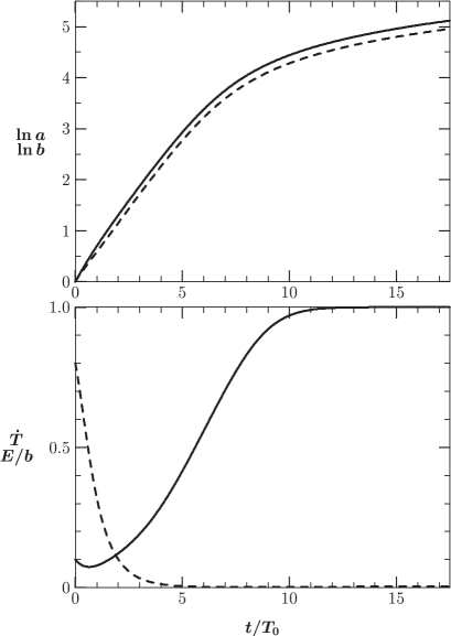
Figure 1: A numerical solution with initial conditions $T_{i}=\dot{T}_{i}=0.1$, $E_{i}=0.8$. In upper figure, solid and dashed lines are e-foldings of scale factors $a$ and $b$, respectively. In lower figure, the solid line is $\dot{T}$ and the dashed line is $E/b$.

We showed the numerical solutions for $p=3$ case in FIG. 1 and FIG. 2. The general behavior is that as the universe expands the electric field vanishes quickly and tachyon rolling dominates in the end. This occurs in a few e-foldings of scale factor for moderate initial conditions, as shown in FIG. 1. We can also think of rather extreme initial conditions. In FIG. 2, we showed the solution for tiny value of $T_{i}$ and $\dot{T}_{i}$ and nearly critical value of $E_{i}$. Near the top of the potential, the existence of critical electric field gives a rapid expansion due to the huge energy density it has. However the electric field itself dies exponentially and the final e-folding of scale factor seems not very significant, unless serious fine tuning is involved. For example, we obtained about 5 additional e-foldings in FIG. 1 from a fine tuning of $\sqrt{1-\dot{T}_{i}^{2}-E_{i}^{2}}=10^{-5}$, compared to the case $E_{i}=0$. The existence of critical electric field is not more helpful than the fine tuning of initial values of tachyon field as far as inflation is concerned.

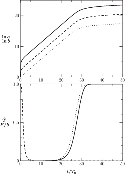
Figure 2: A solution with fine tuned initial condition $T_{i}=\dot{T}_{i}=\sqrt{1-\dot{T}_{i}^{2}-E_{i}^{2}}=10^{-5}$. Solid and dashed lines are same as FIG. 1. Dotted lines are e-folding of scale factor $a$ and $\dot{T}$, in the case of $E_{i}=0$ with same $T_{i}$ and $\dot{T}_{i}$.

VII Concluding Remarks

In this paper we have discussed a few topics of tachyon driven cosmology based on cosmological time-dependent solutions so-called rolling tachyons describing the homogeneous decay of unstable space-filling D-brane. In relation with the issue of inflation, it seems unlikely to provide sufficient e-folding by any runaway tachyon potential. Addition of linear dilaton or Born-Infeld electromagnetic fields is not enough to prolong sufficiently the period of inflation without a fine-tuning.

Though we have dealt with the cosmological solutions without spatial dependence, such solutions with both time and spatial dependence should be studied in relation with cosmological density fluctuation. As a viable source of density perturbation, various stable D-branes of codimension-one or -two or composites of D-brane-fundamental string have been proposed as static configurations Sen:2003tm ; Lambert:2003zr ; Kim:2003in because of the absence of perturbative open string degrees after the decay of unstable D-brane. Until now, on the cosmological density perturbation due to tachyon, there exist both bad news like caustics Felder:2002sv and recent good news based on numerical analysis Felder:2004xu .

- (1) A. Sen, JHEP 0204, 048 (2002) [arXiv:hep-th/0203211]; A. Sen, JHEP 0207, 065 (2002) [arXiv:hep-th/0203265].
- (2) A. Sen, Mod. Phys. Lett. A 17, 1797 (2002) [arXiv:hep-th/0204143].
- (3) G. W. Gibbons, Phys. Lett. B 537, 1 (2002) [arXiv:hep-th/0204008].
- (4) M. Fairbairn and M. H. G. Tytgat, Phys. Lett. B 546, 1 (2002) [arXiv:hep-th/0204070]; S. Mukohyama, Phys. Rev. D 66, 024009 (2002) [arXiv:hep-th/0204084]; A. Feinstein, Phys. Rev. D 66, 063511 (2002) [arXiv:hep-th/0204140]; T. Padmanabhan, Phys. Rev. D 66, 021301 (2002) [arXiv:hep-th/0204150]; A. V. Frolov, L. Kofman and A. A. Starobinsky, Phys. Lett. B 545, 8 (2002) [arXiv:hep-th/0204187]; D. Choudhury, D. Ghoshal, D. P. Jatkar and S. Panda, Phys. Lett. B 544, 231 (2002) [arXiv:hep-th/0204204]; X. z. Li, J. g. Hao and D. j. Liu, Chin. Phys. Lett. 19, 1584 (2002) [arXiv:hep-th/0204252]; G. Shiu and I. Wasserman, Phys. Lett. B 541, 6 (2002) [arXiv:hep-th/0205003]; L. Kofman and A. Linde, JHEP 0207, 004 (2002) [arXiv:hep-th/0205121]; H. B. Benaoum, arXiv:hep-th/0205140; M. Sami, Mod. Phys. Lett. A 18, 691 (2003) [arXiv:hep-th/0205146]; M. Sami, P. Chingangbam and T. Qureshi, Phys. Rev. D 66, 043530 (2002) [arXiv:hep-th/0205179]; J. c. Hwang and H. Noh, Phys. Rev. D 66, 084009 (2002) [arXiv:hep-th/0206100]; Y. S. Piao, R. G. Cai, X. m. Zhang and Y. Z. Zhang, Phys. Rev. D 66, 121301 (2002) [arXiv:hep-ph/0207143]; G. Shiu, S. H. H. Tye and I. Wasserman, Phys. Rev. D 67, 083517 (2003) [arXiv:hep-th/0207119]; X. z. Li, D. j. Liu and J. g. Hao, arXiv:hep-th/0207146; J. M. Cline, H. Firouzjahi and P. Martineau, JHEP 0211, 041 (2002) [arXiv:hep-th/0207156]; S. Mukohyama, Phys. Rev. D 66, 123512 (2002) [arXiv:hep-th/0208094]; M. C. Bento, O. Bertolami and A. A. Sen, Phys. Rev. D 67, 063511 (2003) [arXiv:hep-th/0208124]; J. g. Hao and X. z. Li, Phys. Rev. D 66, 087301 (2002) [arXiv:hep-th/0209041]; J. S. Bagla, H. K. Jassal and T. Padmanabhan, Phys. Rev. D 67, 063504 (2003) [arXiv:astro-ph/0212198]; M. Sami, P. Chingangbam and T. Qureshi, Pramana 62, 765 (2004) [arXiv:hep-th/0301140]; N. Ohta, Phys. Rev. Lett. 91, 061303 (2003) [arXiv:hep-th/0303238]; A. Das and A. DeBenedictis, arXiv:gr-qc/0304017; R. Emparan and J. Garriga, JHEP 0305, 028 (2003) [arXiv:hep-th/0304124]; D. Choudhury, D. Ghoshal, D. P. Jatkar and S. Panda, JCAP 0307, 009 (2003) [arXiv:hep-th/0305104]; S. Nojiri and S. D. Odintsov, Phys. Lett. B 571, 1 (2003) [arXiv:hep-th/0306212]; A. Steer and F. Vernizzi, arXiv:hep-th/0310139; V. Gorini, A. Y. Kamenshchik, U. Moschella and V. Pasquier, arXiv:hep-th/0311111; H. Q. Lu, arXiv:hep-th/0312082; A. Sen, arXiv:hep-th/0312153; G. Calcagni, Phys. Rev. D 69, 103508 (2004) [arXiv:hep-ph/0402126]; N. Barnaby and J. M. Cline, Phys. Rev. D 70, 023506 (2004) [arXiv:hep-th/0403223]; J. Y. Kim, J. Korean Phys. Soc. 42, S78 (2003) ; Y. Kim, C. Y. Oh, and N. Park, J. Korean Phys. Soc. 42, 573 (2003); S.-W. Kim, J. Korean Phys. Soc. 42, S94 (2003).
- (5) G. N. Felder, L. Kofman and A. Starobinsky, JHEP 0209, 026 (2002) [arXiv:hep-th/0208019].
- (6) T. Mehen and B. Wecht, JHEP 0302, 058 (2003) [arXiv:hep-th/0206212].
- (7) C. Kim, H. B. Kim and Y. Kim, Phys. Lett. B 552, 111 (2003) [arXiv:hep-th/0210101].
- (8) G. W. Gibbons, Class. Quant. Grav. 20, S321 (2003) [arXiv:hep-th/0301117].
- (9) C. Kim, H. B. Kim, Y. Kim and O-K. Kwon, proceedings of PAC Memorial Symposium on Theoretical Physics, pp.209-239 (Chungbum Publishing House, Seoul, 2003), arXiv:hep-th/0301142.
- (10) A. Mazumdar, S. Panda and A. Perez-Lorenzana, Nucl. Phys. B 614, 101 (2001) [arXiv:hep-ph/0107058].
- (11) J. McGreevy and H. Verlinde, JHEP 0312, 054 (2003) [arXiv:hep-th/0304224].
- (12) J. L. Karczmarek and A. Strominger, arXiv:hep-th/0309138.
- (13) A. A. Gerasimov and S. L. Shatashvili, JHEP 0010, 034 (2000) [arXiv:hep-th/0009103]; D. Kutasov, M. Marino and G. W. Moore, JHEP 0010, 045 (2000) [arXiv:hep-th/0009148]; D. Kutasov, M. Marino and G. W. Moore, arXiv:hep-th/0010108.
- (14) A. Buchel, P. Langfelder and J. Walcher, Annals Phys. 302, 78 (2002) [arXiv:hep-th/0207235].
- (15) C. Kim, H. B. Kim, Y. Kim and O-K. Kwon, JHEP 0303, 008 (2003) [arXiv:hep-th/0301076].
- (16) F. Leblond and A. W. Peet, JHEP 0304, 048 (2003) [arXiv:hep-th/0303035].
- (17) C. Kim, Y. Kim, O-K. Kwon and C. O. Lee, JHEP 0311, 034 (2003) [arXiv:hep-th/0305092].
- (18) N. Lambert, H. Liu and J. Maldacena, arXiv:hep-th/0303139.
- (19) C. Kim, Y. Kim and C. O. Lee, JHEP 0305, 020 (2003) [arXiv:hep-th/0304180].
- (20) C. Kim, Y. Kim, O-K. Kwon and P. Yi, JHEP 0309, 042 (2003) [arXiv:hep-th/0307184].
- (21) D. Kutasov and V. Niarchos, Nucl. Phys. B 666, 56 (2003) [arXiv:hep-th/0304045].
- (22) K. Okuyama, JHEP 0305, 005 (2003) [arXiv:hep-th/0304108].
- (23) A. Sen, JHEP 9809, 023 (1998) [arXiv:hep-th/9808141].
- (24) A. Sen, JHEP 9812, 021 (1998) [arXiv:hep-th/9812031].
- (25) A. Sen, Phys. Rev. D 68, 106003 (2003) [arXiv:hep-th/0305011].
- (26) C. Kim, Y. Kim and O. K. Kwon, arXiv:hep-th/0404163.
- (27) P. Horava, Adv. Theor. Math. Phys. 2, 1373 (1999) [arXiv:hep-th/9812135].
- (28) M. Gutperle and A. Strominger, Phys. Rev. D 67, 126002 (2003) [arXiv:hep-th/0301038].
- (29) P. Mukhopadhyay and A. Sen, JHEP 0211, 047 (2002) [arXiv:hep-th/0208142]; G. Gibbons, K. Hashimoto and P. Yi, JHEP 0209, 061 (2002) [arXiv:hep-th/0209034]; O-K. Kwon and P. Yi, JHEP 0309, 003 (2003) [arXiv:hep-th/0305229]; H. U. Yee and P. Yi, arXiv:hep-th/0402027.
- (30) A. Sen, Phys. Rev. D 68, 066008 (2003) [arXiv:hep-th/0303057].
- (31) G. N. Felder and L. Kofman, arXiv:hep-th/0403073.
- (32) H. w. Lee and W. S. l’Yi, J. Korean Phys. Soc. 43, 676 (2003) [arXiv:hep-th/0210221]; J. H. Chung and W. S. L’Yi, J. Korean Phys. Soc. 45, 318 (2004).