Cosmology as Geodesic Motion

Abstract

For gravity coupled to $N$ scalar fields, with arbitrary potential $V$, it is shown that all flat (homogeneous and isotropic) cosmologies correspond to geodesics in an $(N+1)$-dimensional ‘augmented’ target space of Lorentzian signature $(1,N)$, timelike if $V>0$, null if $V=0$ and spacelike if $V<0$. Accelerating cosmologies correspond to timelike geodesics that lie within an ‘acceleration subcone’ of the ‘lightcone’. Non-flat ($k=\pm 1$) cosmologies are shown to evolve as projections of geodesic motion in a space of dimension $(N+2)$, of signature $(1,N+1)$ for $k=-1$ and signature $(2,N)$ for $k=+1$. This formalism is illustrated by cosmological solutions of models with an exponential potential, which are comprehensively analysed; the late-time behaviour for other potentials of current interest is deduced by comparison.

1 Introduction

Cosmological models with scalar field matter have been much studied in the context of inflation and, more recently, in the context of the late-time acceleration that is indicated by current astronomical observations (see [1] for a recent review). One theoretical motivation for these studies is that scalar fields arise naturally from the compactification of higher-dimensional theories, such as string or M-theory. However, the type of scalar field potential obtained in these compactifications is sufficiently restrictive that until recently it was considered to be difficult to get accelerating cosmologies in this way, although the existence of an accelerating phase in a hyperbolic ($k=-1$) universe obtained by compactification had been noted [2], and non-perturbative effects in M-theory have since been shown to allow unstable de Sitter vacua [3].

In an earlier paper, we pointed out that compactification on a compact hyperbolic manifold with a time-dependent volume modulus naturally leads to a flat ($k=0$) expanding universe that undergoes a transient period of accelerating expansion [4]. Numerous subsequent studies have shown that such cosmological solutions are typical to all compactifications that involve compact hyperbolic spaces or non-vanishing $p$-form field strengths (flux) [5, 6, 7, 8, 9, 10], and this was additionally confirmed in a systematic study [11]. Furthermore, the transient acceleration in these models is easily understood [12] in terms of the positive scalar field potential that both hyperbolic and flux compactifications produce in the effective, lower-dimensional, action. This perspective also makes clear the generic nature of transient acceleration.

For any realistic application one would want the lower-dimensional spacetime to be four-dimensional, but for theoretical studies it is useful to consider a general $d$-dimensional spacetime. Assuming that we have gravity, described by a metric $g_{mn}$, coupled to $N$ scalar fields $\bm{\phi}$ taking values in a Riemannian target space with metric $G_{\alpha\beta}$ and with potential energy $V$, the effective action must take the form

$$\int d^{d}x\,\sqrt{-g}\left(\frac{1}{4}R-\frac{1}{2}g^{mn}G_{\alpha\beta}(\bm{\phi})\partial_{m}\phi^{\alpha}\partial_{n}\phi^{\beta}-V(\bm{\phi})\right)$$ (1)

where $R$ is the (spacetime) Ricci scalar. We are interested in solutions of the field equations of the action (1) for which the line element has the Friedmann-Lemaître-Robertson-Walker (FLRW) form for a homogeneous and isotropic spacetime. In standard coordinates,

$$ds^{2}=-dt^{2}+S(t)^{2}d\Sigma_{k}^{2}\,,$$ (2)

where the function $S(t)$ is the scale factor, and $\Sigma_{k}$ represents the $(d-1)$-dimensional spatial sections of constant curvature $k$. We normalise $k$ such that it may take values $k=0,\pm 1$ for a Riemann tensor $\bar{R}_{\bar{m}\bar{n}\bar{o}\bar{p}}=k\left(\bar{g}_{\bar{m}\bar{o}}\bar{g}_{\bar{n}\bar{p}}-\bar{g}_{\bar{m}\bar{p}}\bar{g}_{\bar{n}\bar{o}}\right)$ with metric $\bar{g}$ on $\Sigma_{k}$. The scalar fields are taken to depend only on time, which is the only choice compatible with the symmetries of FLRW spacetimes. The universe is expanding if $\partial_{t}S>0$ and accelerating if $\partial_{t}^{2}S>0$. We need only discuss expanding cosmologies because contracting cosmologies are obtained by time-reversal.

In some simple cases, the target space has a one-dimensional factor parametrised by a dilaton field $\varphi(\bm{\phi})$, and the potential takes the form

$$V=V_{0}\,e^{-2a\varphi}$$ (3)

for some ‘dilaton coupling’ constant $a$ and constant $V_{0}$. This model is of special interest, in part because of its amenability to analysis. The special case for which the dilaton is the only scalar field was analysed many years ago (for $V_{0}>0$) using the observation that, for an appropriate choice of time variable, cosmological solutions correspond to trajectories in the ‘phase-plane’ parametrised by the first time-derivatives of the dilaton and the scale factor [13]. This method (which has recently been extended to potentials that are the sum of two exponentials [14]) allows a simple visualisation of all possible cosmological trajectories. Moreover, all trajectories for flat cosmologies can be found explicitly [15, 16] (see also [17, 18, 19]), and a related method allows a visualisation of their global nature [20, 21]. It was noted in [13] that there is both a ‘critical’ and a ‘hypercritical’ value of the dilaton coupling constant $a$, at which the set of trajectories undergoes a qualitative change. In spacetime dimension $d$, these values are [15, 11]

$$\alpha_{c}=\sqrt{\frac{2}{d-2}}\qquad\textrm{and}\qquad\alpha_{h}=\sqrt{\frac{2(d-1)}{d-2}}\,.$$ (4)

Below the critical value ($a<\alpha_{c}$) there exists a late-time attractor universe undergoing accelerating expansion, whereas only transient acceleration is possible above it. The hypercritical coupling ($a=\alpha_{h}$) separates ‘steep’ exponential potentials (which arise in flux compactifications) and ‘gentle’ exponential potentials (which arise from hyperbolic compactification, in which case $a>\alpha_{c}$ so the potential is still too steep to allow eternal acceleration). One aim of this paper is to generalise this type of analysis to the multi-scalar case. For $k=0$, this has been done already for what could be called a ‘multi-dilaton’ model [22], and for the multi-scalar model with exponential potential (3) [23]. Here we consider all cosmological trajectories (arbitrary $k$) for an exponential potential of either sign, and for any spacetime dimension $d$. In particular, we find exact solutions for all flat cosmologies when $V<0$, following the method used in [16] for $V>0$, and the exact phase-plane trajectories for all $k$ when $V=V_{0}<0$.

A more ambitious aim of this paper is to determine what can be said about cosmologies with more general scalar potentials. What kind of model-independent behaviour can one expect, and how generic is the phenomenon of transient acceleration? Exponential potentials are simple partly because of the power-law attractor cosmologies that they permit, but such simple solutions do not occur for other potentials so other methods are needed. In this paper, we develop an alternative method of visualising cosmological solutions that applies to any potential, and we illustrate it by an application to exponential potentials. As we explain, exponential potentials serve as ‘reference potentials’ in determining the late-time behaviour of cosmologies arising in a large class of models with other potentials.

Our starting point for the new formalism is the observation [25] that flat cosmological solutions of gravity coupled to $N$ scalar fields with $V=0$ can be viewed as null geodesics in an ‘augmented’ target space of dimension $N+1$ with a metric of Lorentzian signature (see [26] for related results). Trajectories in this space corresponding to non-flat cosmologies are neither null nor geodesic. However, we will see that they are projections of null geodesics in a ‘doubly-augmented’ target space with a metric of signature $(1,N+1)$ for $k=-1$ and signature $(2,N)$ for $k=+1$.

It turns out that the extension of these results to $V\neq 0$ is very simple. Flat cosmologies are again geodesics in the augmented target space but with respect to a conformally rescaled metric; the geodesic is timelike if $V>0$ and spacelike if $V<0$. Null geodesics are unaffected by the conformal rescaling and hence continue to correspond to ($k=0$) cosmologies for $V=0$. The analysis of acceleration is also simple in this framework: within the lightcone is an ‘acceleration cone’, and if a geodesic enters its acceleration cone then the corresponding universe will accelerate. In the case of a flat target space with an exponential potential, the fixed point geodesics are just straight lines, and the universe is accelerating if the straight line lies within the acceleration cone. The further extension to $k\neq 0$ cosmologies is achieved exactly as in the $V=0$ case. Cosmological trajectories are projections of geodesics in the doubly-augmented target space with respect to a conformally rescaled metric of signature $(1,N+1)$ for $k=-1$ and $(2,N)$ for $k=+1$. The geodesic is timelike if $V>0$, null if $V=0$ and spacelike if $V<0$.

The plan of this paper is as follows. Section 2 reviews, in our conventions, the equations of motion in multi-scalar cosmologies, and we derive a useful alternative criterion for the acceleration of the scale factor. In section 3, we consider possible fixed points, concluding that these occur only for exponential potentials, and we determine the nature of these fixed points for arbitrary $d$, $k$ and sign of the potential. In section 4 we discuss the phase-plane trajectories and present some exact $V<0$ solutions. In section 5 we develop the interpretation of multi-scalar cosmologies as geodesic motion. In section 6 we introduce the notion of the acceleration cone, and we show how the cosmologies arising in exponential-potential models fit into the new framework; other potentials of current interest are also considered. We summarise in section 7.

2 Multi-Scalar Cosmologies

We begin by briefly reviewing the equations of motion for multi-scalar cosmologies that follow from the action (1). These equations will be given in two different forms, distinguished by the choice of time coordinate. The second form will be useful to our analysis in the next section of possible ‘fixed points’, which correspond to power-law cosmologies in the first form.

To simplify the equations we define

$$\left(D_{t}^{2}\phi\right)^{\alpha}:=\partial_{t}^{2}\phi^{\alpha}+\Gamma^{\alpha}{}_{\beta\gamma}\partial_{t}\phi^{\beta}\partial_{t}\phi^{\gamma}$$ (5)

where $\Gamma^{\alpha}{}_{\beta\gamma}$ is the Levi-Cività connection for the target space metric $G$, and we introduce the following ‘characteristic functions’ of the potential V:

$$a_{\alpha}(\bm{\phi})=-{1\over 2}{\partial\ln|V|\over\partial\phi^{\alpha}}\,.$$ (6)

These are the components of a 1-form on the target space dual to a vector field $\mathbf{a}$. In a vector notation, the scalar field equation can now be written as

$$D_{t}^{2}{\bm{\phi}}+\left(d-1\right)H\,\partial_{t}{\bm{\phi}}=2V\mathbf{a}\,,$$ (7)

where $H(t)=\partial_{t}S/S$ is the Hubble function. The Friedmann constraint is

$$S^{2}\left[|\partial_{t}{\bm{\phi}}|^{2}+2V-\left(d-1\right)\alpha_{c}^{-2}H^{2}\right]=\left(d-1\right)\alpha_{c}^{-2}k,$$ (8)

where the norm $|\partial_{t}{\bm{\phi}}|$ (and hence the inner product) is the one induced by the target space metric: $|\partial_{t}{\bm{\phi}}|^{2}=\partial_{t}{\bm{\phi}}\cdot\partial_{t}{\bm{\phi}}=G_{\alpha\beta}\,\partial_{t}\phi^{\alpha}\partial_{t}\phi^{\beta}$. Differentiating the Friedmann constraint, and using the scalar field equation (7), we deduce the ‘acceleration equation’

$$\partial_{t}^{2}S={2S\over d-1}\left[\alpha_{c}^{2}V-|\partial_{t}{\bm{\phi}}|^{2}\right],$$ (9)

where we recall that $\alpha_{c}$ is the ‘critical’ constant given in (4). Clearly, acceleration is possible only if $V>0$. Note too that $H(t)$ cannot vanish unless either $V<0$ or $k>0$ (or $V=0$, $k=0$ and $|\partial_{t}{\bm{\phi}}|=0$) so only in these cases can an expanding universe recollapse.

For the following section, it will prove useful to rewrite the above equations in terms of a new time coordinate $\tau$, defined as a function of $t$ by the relation

$$d\tau=|V|^{1\over 2}dt\,.$$ (10)

Note that we have allowed for the possibility that $V<0$, although $V=0$ is excluded. We will also set

$$S(t)=e^{\beta(\tau)}\,.$$ (11)

In terms of the variable $\beta$, the condition $\partial_{t}S>0$ for expansion is $\dot{\beta}>0$, while the condition $\partial_{t}^{2}S>0$ for acceleration is

$$\ddot{\beta}+\dot{\beta}^{2}-\dot{\beta}\,\left(\mathbf{a}\cdot\dot{\bm{\phi}}\right)>0\,,$$ (12)

where the overdot denotes differentiation with respect to $\tau$.

In the new time coordinate, the scalar field equation becomes

$$D_{\tau}^{2}{\bm{\phi}}=\left(\mathbf{a}\cdot\dot{\bm{\phi}}\right)\dot{\bm{\phi}}-\left(d-1\right)\dot{\beta}\,\dot{\bm{\phi}}+2\,{\rm sign}\,V\,\mathbf{a}\,,$$ (13)

and the Friedmann constraint becomes

$$e^{2\beta}|V|\left[|\dot{\bm{\phi}}|^{2}-\left(d-1\right)\alpha_{c}^{-2}\dot{\beta}^{2}+2\,{\rm sign}\,V\right]=\left(d-1\right)\alpha_{c}^{-2}k\,.$$ (14)

The acceleration equation is now

$$\ddot{\beta}=-{2\over d-1}|\dot{\bm{\phi}}|^{2}-\dot{\beta}^{2}+\dot{\beta}\left(\mathbf{a}\cdot\dot{\bm{\phi}}\right)+{2\alpha_{c}^{2}\over d-1}\,{\rm sign}\,V\,,$$ (15)

and the condition (12) for acceleration is therefore equivalent to

$$|\dot{\bm{\phi}}|^{2}<\alpha_{c}^{2}\,\textrm{sign}\,V\,.$$ (16)

Note that this inequality is independent of $k$, and hence valid for all $k$. As expected, it can be satisfied only if $V>0$.

3 Fixed Points

We now wish to determine whether the system of equations (13, 15) subject to the constraint (14), admits any fixed point solutions for which

$$\ddot{\beta}=0\qquad\textrm{and}\qquad D_{\tau}^{2}{\bm{\phi}}=\mathbf{0}\,.$$ (17)

We shall see that these conditions are consistent only for exponential potentials, for which the equations (13, 15) become those of an autonomous dynamical system, and we determine the fixed points and their type for all $d$, $k$ and for either sign of the potential. For this analysis, it is convenient to introduce the quantity

$$\omega=\sqrt{{|\alpha_{h}^{2}-a^{2}|\over 2}}\,,\qquad a=|\mathbf{a}|\,.$$ (18)

Recall that $\alpha_{h}$ is the ‘hypercritical’ constant given in (4).

3.1 Fixed Point Conditions

Given $D_{\tau}^{2}{\bm{\phi}}=0$, equation (13) yields

$$\dot{\bm{\phi}}=c\mathbf{a}\qquad\left(\Rightarrow\ \ |\dot{\bm{\phi}}|^{2}=c^{2}a^{2},\ \ \mathbf{a}\cdot\dot{\bm{\phi}}=c\,a^{2}\right),$$ (19)

where $c$ solves the quadratic equation

$$a^{2}c^{2}-\left(d-1\right)c\dot{\beta}+2\,\,{\rm sign}\,V=0\,.$$ (20)

Given $\ddot{\beta}=0$, equation (15) yields

$$2\,{\rm sign}\,V = \left(d-2\right)|\dot{\bm{\phi}}|^{2}+{1\over 2}\left(d-1\right)\left(d-2\right)\left[\dot{\beta}^{2}-\dot{\beta}\left(\mathbf{a}\cdot\dot{\bm{\phi}}\right)\right]$$ (21)

$$= \left(d-2\right)c^{2}a^{2}+{1\over 2}\left(d-1\right)\left(d-2\right)\left[\dot{\beta}^{2}-ca^{2}\dot{\beta}\right]$$

where we have used (19) to get to the second line. Using this equation to eliminate the $2\,{\rm sign}\,V$ term from (20) we arrive at the quadratic equation

$$\left(\dot{\beta}-a^{2}c\right)\left(\dot{\beta}-\alpha_{c}^{2}c\right)=0\,.$$ (22)

There are therefore two types of fixed point:

• $\dot{\beta}=\alpha_{c}^{2}c$. Using this in (20) we deduce that $a\neq\alpha_{h}$ and that

  $$c^{2}={2\,{\rm sign}\,V\over\left(\alpha_{h}^{2}-a^{2}\right)}\,.$$ (23)

  This requires

  $$\!\!\!\!\!\!\!\!\!\!\!\!\!EITHER\ \ \ V>0\ {\rm and}\ a<\alpha_{h}\,,\qquad OR\ \ \ V<0\ {\rm and}\ a>\alpha_{h}\,,$$ (24)

  and

  $$\omega\,\dot{\bm{\phi}}=\pm\mathbf{a}\,,\qquad\omega\,\dot{\beta}=\pm\alpha_{c}^{2}\,.$$ (25)

  It then follows that

  $$|\dot{\bm{\phi}}|^{2}-\left(d-1\right)\alpha_{c}^{-2}\dot{\beta}^{2}+2\,{\rm sign}\,V=0\,.$$ (26)

  This is just the Friedmann constraint for $k=0$, so this type of fixed point occurs only for $k=0$.

• $\dot{\beta}=a^{2}c$. Using this in (20) we deduce that

  $$c^{2}={\alpha_{c}^{2}\over a^{2}}\ {\rm sign}\,V\,.$$ (27)

  It follows that this type of fixed point can occur only for $V>0$, and that

  $$\dot{\bm{\phi}}=\pm\left({\alpha_{c}\over a}\right)\mathbf{a}\,,\qquad\dot{\beta}=\pm\alpha_{c}a\,.$$ (28)

  Using this in the Friedmann constraint we deduce that

  $$\alpha_{c}^{-2}k=e^{2\beta}|V|\left(\alpha_{c}^{2}-a^{2}\right).$$ (29)

  We may exclude the possibility that $a=\alpha_{c}$ because this yields a $k=0$ fixed point of the type already considered, so $k\neq 0$ and we need $k>0$ for $a<\alpha_{c}$ and $k<0$ for $a>\alpha_{c}$. Note that $|\dot{\bm{\phi}}|=\alpha_{c}$ for this type of fixed point, so the fixed point cosmology is neither accelerating nor decelerating.

3.2 Determination of the fixed point type

The above results are in complete analogy with those of [13, 15] for the one-scalar case. To see why, it should first be appreciated that the fixed point conditions have been derived on the assumption that $\dot{\beta}$ is constant, and that $\dot{\bm{\phi}}$ is covariantly constant. It then follows from (19, 20) that $\mathbf{a}$ must be covariantly constant too. However, for any space that admits a non-zero covariantly constant vector, there exist coordinates in which this vector is constant, not just covariantly constant. For coordinates in which $\mathbf{a}$ is constant the potential takes the form

$$V=V_{0}\,e^{-2\mathbf{a}\cdot{\bm{\phi}}}\,,$$ (30)

which is of the form (3) with $a\varphi=\mathbf{a}\cdot{\bm{\phi}}$. Moreover, for any target space on which this potential is globally defined, one can find new coordinates such that

$$G_{\alpha\beta}\,d\phi^{\alpha}d\phi^{\beta}=d\varphi^{2}+\widehat{G}_{\widehat{\alpha}\widehat{\beta}}\left(\chi\right)\,d\chi^{\widehat{\alpha}}d\chi^{\widehat{\beta}}\,,$$ (31)

where $\widehat{G}$ is a metric on a ‘reduced’ target space with $(N-1)$ coordinates $\chi$. In these target space coordinates, the scalar field equations are

$$D_{\tau}^{2}\chi = a\dot{\varphi}\dot{\chi}-\left(d-1\right)\dot{\beta}\,\dot{\chi}\,,$$

$$\ddot{\varphi} = a\dot{\varphi}^{2}-\left(d-1\right)\dot{\beta}\dot{\varphi}+2a\,{\rm sign}\,V\,,$$ (32)

and the Friedmann constraint is

$$\alpha_{c}^{2}\left[|\dot{\chi}|^{2}+\dot{\varphi}^{2}+2\,\textrm{sign}\,V_{0}\right]-\left(d-1\right)\dot{\beta}^{2}=k\left(d-1\right)e^{2\left(a\varphi-\beta\right)}|V_{0}|^{-1}\,.$$ (33)

These imply the acceleration equation for $\ddot{\beta}$. If we suppose that the reduced target space is flat then the scalar field equations, together with the acceleration equation, define an autonomous dynamical system:

$$\ddot{\varphi} = a\dot{\varphi}^{2}-\left(d-1\right)\dot{\beta}\dot{\varphi}+2a\,{\rm sign}\,V\,,$$

$$\ddot{\beta} = -{2\over\left(d-1\right)}\,\left[\dot{\varphi}^{2}+|\dot{\chi}|^{2}-\alpha_{c}^{2}\,{\rm sign}\,V\right]-\dot{\beta}^{2}+a\dot{\beta}\dot{\varphi}\,,$$

$$\ddot{\chi} = a\dot{\varphi}\,\dot{\chi}-\left(d-1\right)\dot{\beta}\,\dot{\chi}\,.$$ (34)

Note that we may consistently set $\dot{\chi}=0$ to recover the equations of the one-scalar model. As there are no fixed points with $\dot{\chi}\neq 0$, the fixed points of the multi-scalar model are the same as those of the one-scalar model.

If the reduced target space is not flat then a connection term must be added to the last equation in (3.2). As this introduces dependence on $\chi$, the equations no longer define an autonomous dynamical system in just $N+1$ variables. It is not clear how much difference this makes to the results: note that the connection term has no effect on the stability of fixed points with $\dot{\chi}=0$ because it is quadratic in $\dot{\chi}$. However, we will suppose for the analysis to follow that the reduced target space is flat. We may then assume with no essential loss of generality that it is also one-dimensional (i.e. $N=2$) so we have an autonomous dynamical system for just three variables. We linearise about a fixed point with $\dot{\varphi}=\dot{\varphi}_{0}$ and $\dot{\beta}=\dot{\beta}_{0}$ by writing

$$\dot{\varphi}=\dot{\varphi}_{0}+x\,,\qquad\dot{\beta}=\dot{\beta}_{0}+y\,,\qquad\dot{\chi}=z\,.$$ (35)

The linearised equations for $(x,y,z)=U^{T}$ take the form $\dot{U}=MU$, where $M$ is the $3\times 3$ matrix

$$\pmatrix{2a\dot{\varphi}_{0}-\left(d-1\right)\dot{\beta}_{0}&-\left(d-1\right)\dot{\varphi}_{0}&0\cr a\dot{\beta}_{0}-4\left(d-1\right)^{-1}\dot{\varphi}_{0}&a\dot{\varphi}_{0}-2\dot{\beta}_{0}&0\cr 0&0&a\dot{\varphi}_{0}-\left(d-1\right)\dot{\beta}_{0}}.$$ (36)

The eigenvalues of this matrix determine the nature of the fixed point. We consider the two types of fixed point in turn:

• $k=0$. In this case

  $$\omega\dot{\varphi}_{0}=\pm a\,,\qquad\omega\dot{\beta}_{0}=\pm\alpha_{c}^{2}\,.$$ (37)

  The eigenvalues of $M$ are

  $$\pm 2\omega^{-1}\left(a^{2}-\alpha_{c}^{2}\right),\qquad\pm\omega^{-1}\left(a^{2}-\alpha_{h}^{2}\right),\qquad\pm\omega^{-1}\left(a^{2}-\alpha_{h}^{2}\right).$$ (38)

  For an expanding universe we must take the top sign (corresponding, for $V>0$, to the upper branch of the $k=0$ hyperboloid). Then we have a stable node (all eigenvalues real and negative) for $a<\alpha_{c}$. For $\alpha_{c}<a<\alpha_{h}$ we have a saddle, with one real-negative and two real-positive eigenvalues; the instability due to the positive eigenvalues is what leads to the ‘flatness problem’ of standard big-bang cosmology.

  For $V<0$ we may have $a>\alpha_{h}$, in which case the fixed point is an unstable node (all eigenvalues real and positive). All $k=-1$ trajectories start at this unstable fixed point and end at the stable fixed point on the other branch of the $k=0$ hyperboloid; as $\dot{\beta}<0$ at this other fixed point, all $k=-1$ universes recollapse to a big crunch singularity. However, for $a\gg\alpha_{h}$ there is a long quasi-static period on some of these trajectories.

• $k\neq 0$. In this case

  $$\dot{\varphi}_{0}=\pm\alpha_{c}\,,\qquad\dot{\beta}_{0}=\pm\alpha_{c}a\,.$$ (39)

  The eigenvalues of $M$ are

  $$\!\!\!\pm{\alpha_{c}\over 2}\left[-\left(d-2\right)a+\sigma\sqrt{16-\left(d-2\right)\left(10-d\right)a^{2}}\right],\qquad\mp 2a/\alpha_{c}\,,$$ (40)

  where $\sigma=1$ for one eigenvalue and $-1$ for another. Take the top sign again. For $a\leq\alpha_{c}$ all eigenvalues are real but one is positive and the others negative, so we have a saddle point. For $a>\alpha_{c}$ all eigenvalues are real and negative provided either $d\geq 10$ or (if $d\leq 9$)

  $$a\leq\bar{a}\equiv{4\over\sqrt{\left(d-2\right)\left(10-d\right)}}\,.$$ (41)

  Otherwise (i.e. $d\leq 9$ and $a>\bar{a}$) we have one real negative eigenvalue and two complex eigenvalues with negative real parts, and hence a stable ‘spiral-node’ (a spiral in the $xy$ plane and a node in the $z$ direction). Note that

  $$\alpha_{c}<\bar{a}\leq\alpha_{h}$$ (42)

  where the equality occurs for $d=9$. Thus, for any $d$ the $k\neq 0$ fixed point is an unstable saddle if $a<\alpha_{c}$, and is stable for $a>\alpha_{c}$ but can be either a node or a spiral-node. For $d\geq 10$ it is always a node, but for $d=9$ it becomes a spiral-node at $a=\alpha_{h}$ and for $d<9$ it becomes a spiral-node at $a=\bar{a}<\alpha_{h}$.

In the supergravity context we are restricted to $d\leq 11$, but there is no scalar potential possible in $d=11$ and the only possible potential in $d=10$ is a positive exponential (with $a>\alpha_{h}$ so there is no fixed-point solution).

4 Phase-Space Trajectories

We now have all the information needed to determine the qualitative behaviour of all phase-space trajectories. We begin with the one-scalar model, obtained by setting $\dot{\chi}\equiv 0$. The trajectories for $V>0$ are sketched in [13] but, for the reader’s convenience, we give a brief summary in words. All $k=0$ trajectories begin, after a big bang singularity, with a period of kinetic energy domination with effectively vanishing potential. For $a>\alpha_{h}$ they end up approaching a similar late-time phase, but for $a<\alpha_{h}$ they approach the $k=0$ fixed-point solution, which is accelerating if $a<\alpha_{c}$ and decelerating if $a>\alpha_{c}$. For $a<\alpha_{c}$, all $k\neq 0$ trajectories sufficiently close to a $k=0$ trajectory also approach the $k=0$ fixed point; in fact, all $k=-1$ trajectories have this property. The behaviour of a $k=+1$ trajectory is determined by its relation to the separatrix of the unstable $k=+1$ fixed point (which is the Einstein Static Universe for $a=0$); those on one side approach the $k=0$ fixed point while those on the other side represent universes that recollapse to a big crunch. For $a>\alpha_{c}$ all $k=+1$ universes recollapse to a big crunch whereas all $k=-1$ universes now approach a zero-acceleration Milne universe (the $k=0$ fixed point now being a saddle point). For $a>\bar{a}$ the $k=-1$ fixed point is an attractor spiral so that all $k=-1$ trajectories spiral around a point of zero-acceleration; as observed in [14], this leads to eternal oscillation between acceleration and deceleration.

For $V<0$ the $k=0$ trajectories were studied in [21] but there seems to be no complete study of all trajectories for this case. We will therefore present some results of the one-scalar model for $V<0$ before moving on to discuss modifications that arise in the multi-scalar case.

4.1 Some Exact $V<0$ Solutions

It is well known that anti-de Sitter space is a solution of Einstein’s equations with a negative cosmological constant. This space must correspond to one of the cosmological trajectories in a model with $V=V_{0}<0$ (which implies that $a=0$). Set

$$\dot{\varphi}=x\,,\qquad\dot{\beta}=y\,,$$ (43)

to get the equations

$$\dot{x}=-\left(d-1\right)xy\,,\qquad\dot{y}=-\left[y^{2}+\lambda^{2}+{2x^{2}\over d-1}\right]$$ (44)

where

$$\lambda={2\over\sqrt{\left(d-1\right)\left(d-2\right)}}\,.$$ (45)

These equations imply that

$$\left[x^{2}-2\lambda^{-2}y^{2}-2\right]=Cx^{2/(d-1)}$$ (46)

for constant $C$. The curves with $C>0$ are the $k=+1$ trajectories and those with $C<0$ are the $k=-1$ trajectories. The two branches of the $C=0$ curve, a hyperbola, are the $k=0$ trajectories. The adS solution corresponds to $C=-\infty$, and hence $x=0$; for this special case we have

$$\dot{y}=-\left[y^{2}+\lambda^{2}\right]$$ (47)

which has the solution $y=-\lambda\tan\lambda\tau$, and hence

$$e^{\beta}=S_{0}\cos\lambda\tau\,.$$ (48)

The Friedmann constraint implies that $k=-1$, as expected, and

$$|V_{0}|={d-1\over 2S_{0}^{2}}\qquad\left[\Rightarrow\lambda\tau={\alpha_{c}t\over|S_{0}|}\right],$$ (49)

and hence

$$ds^{2}=-dt^{2}+S_{0}^{2}\cos^{2}\left(\alpha_{c}t/|S_{0}|\right)d\Sigma_{-1}^{2}\,.$$ (50)

This is anti-de Sitter space. In contrast to de Sitter space, which can be realised (for $V=V_{0}>0$) as a FLRW universe for any $k$ (in particular as the $k=0$ fixed-point solution), anti-de Sitter space is realised as an FLRW cosmology only for $k=-1$, and it does not correspond to a fixed point cosmology (at least in the sense of this paper).

We now turn to the $k=0$ trajectories for arbitrary $a$. In this case we have to solve

$$\dot{x}=-\left(d-1\right)xy+a\left(x^{2}-2\right)$$ (51)

subject to the constraint

$$x^{2}-2\lambda^{-2}y^{2}=2\,.$$ (52)

The constraint is solved by setting

$$x=\sqrt{2}\cosh\xi\,,\qquad y=\lambda\sinh\xi$$ (53)

and the equation of motion becomes

$$\dot{\xi}={1\over\sqrt{2}}\left[\left(a-\alpha_{h}\right)e^{\xi}-\left(a+\alpha_{h}\right)e^{-\xi}\right].$$ (54)

This equation is immediately integrated if $a=\alpha_{h}$. Having found $x,y$ we integrate (43) to deduce that

$$e^{-2\alpha_{h}\varphi}=|\tau|e^{\alpha_{h}^{2}\tau^{2}}\,,\qquad e^{\beta}=S_{0}\left[|\tau|e^{-\alpha_{h}^{2}\tau^{2}}\right]^{1\over 2\left(d-1\right)}\,,$$ (55)

for integration constant $S_{0}$ (we have set to zero the other integration constant as it can be absorbed into $V_{0}$).

If $a\neq\alpha_{h}$ then we introduce the new variable

$$\zeta=\sqrt{\left|{\alpha_{h}-a\over\alpha_{h}+a}\right|}\ e^{\xi}\,.$$ (56)

The two branches of the $k=0$ hyperbola correspond to positive and negative $\zeta$; we take $\zeta>0$. We now consider separately the cases $a>\alpha_{h}$ and $a<\alpha_{h}$:

• $a<\alpha_{h}$. In this case the equation for $\zeta$ is

  $$\dot{\zeta}=-\omega\left(\zeta^{2}+1\right)\qquad\left[\Rightarrow\ \zeta=\cot\omega\tau\right],$$ (57)

  where we recall that $\omega$ is the function of $a$ given in (18). Integration of (43) now leads to

  $$e^{\left(\alpha_{h}^{2}-a^{2}\right)\varphi} = \sin^{\alpha_{h}+a}\omega\tau\ \cos^{a-\alpha_{h}}\omega\tau\,,$$

  $$e^{\beta} = S_{0}\left[\sin^{\alpha_{h}+a}\omega\tau\ \cos^{\alpha_{h}-a}\omega\tau\right]^{{\alpha_{c}^{2}\over 2\alpha_{h}\omega^{2}}}\,.$$ (58)

• $a>\alpha_{h}$. In this case the equation for $\zeta$ is

  $$\dot{\zeta}=\omega\left(\zeta^{2}-1\right).$$ (59)

  There is a fixed point at $\zeta=1$, so we must distinguish between $\zeta>1$ and $\zeta<1$. One finds that

  $$\zeta=\cases{-\coth\omega\tau&$\zeta>1$\cr-\tanh\omega\tau&$\zeta<1$}\,.$$ (60)

  For $\zeta>1$ integration of (43) yields

  $$e^{\left(\alpha_{h}^{2}-a^{2}\right)\varphi} = \sinh^{a+\alpha_{h}}\omega\tau\ \cosh^{a-\alpha_{h}}\omega\tau\,,$$

  $$e^{\beta} = S_{0}\left[\sinh^{a+\alpha_{h}}\omega\tau\ \cosh^{\alpha_{h}-a}\omega\tau\right]^{\alpha_{c}^{2}\over 2\alpha_{h}\omega^{2}}\,.$$ (61)

  For $\zeta<1$ integration of (43) yields

  $$e^{\left(\alpha_{h}^{2}-a^{2}\right)\varphi} = \sinh^{a-\alpha_{h}}\omega\tau\ \cosh^{a+\alpha_{h}}\omega\tau\,,$$

  $$e^{\beta} = S_{0}\left[\sinh^{\alpha_{h}-a}\omega\tau\ \cosh^{a+\alpha_{h}}\omega\tau\right]^{\alpha_{c}^{2}\over 2\alpha_{h}\omega^{2}}\,.$$ (62)

4.2 Multi-scalar Trajectories

In the multi-scalar case, the ‘spectator’ fields $\chi$ have an effect on the scale factor due to the $|\dot{\chi}|^{2}$ term in the acceleration equation, and in the Friedmann constraint (33). Phase space trajectories with non-zero $\dot{\chi}$ will depend on the reduced target space metric but, as long as there are no new fixed points, one may expect the qualitative behaviour to be independent of this metric. Let us therefore continue to suppose that the target space (and hence the reduced target space) is flat. In this case, all $k=0$ trajectories lie in a hyperboloid in phase space that separates the $k=-1$ and $k=+1$ trajectories. This is true for either sign of $V$ but we will now suppose that $V>0$; in this case, we see from (16) that acceleration occurs whenever the phase-plane trajectory enters the region with hyperspherical boundary $|\dot{\bm{\phi}}|=\alpha_{c}$. This was observed in [23] in the context of an analysis of $k=0$ trajectories, but it is also valid for non-zero $k$.

The only exponential models with eternally accelerating cosmological solutions are those for which a fixed point lies inside or on the sphere of acceleration, as happens when $a\leq\alpha_{c}$. For all other values of $a$, any acceleration can be at most transient, and only a subset of the trajectories undergo even transient acceleration; these are the trajectories that pass through the sphere of acceleration. The more scalar fields there are, the more freedom there is to avoid the sphere of acceleration, so transient acceleration in multi-scalar models is less generic than it is in the single-scalar model. To make this statement quantitative would require an understanding, along the lines of [27], of what the appropriate measure might be on the space of trajectories.

The most significant fact about a $k=0$ fixed point is whether it lies inside or outside the sphere of acceleration. Figure 1 illustrates a few examples in a model with two scalar fields and a positive exponential, scalar potential.

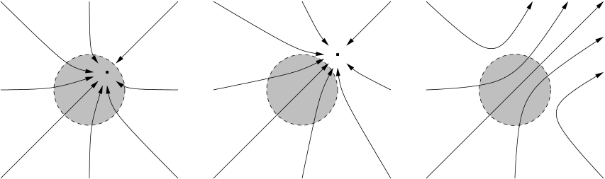
Figure 1: These diagrams for $k=0$ cosmologies with two scalar fields moving in a positive, purely exponential, potential illustrate the trajectories in phase space. The motion takes place in the hyperboloid above the plotted plane, defined by equation (26). The constant characteristic functions $\mathbf{a}$ of the potential satisfy $a<\alpha_{c}$, $\alpha_{c}<a<\alpha_{h}$ and $a>\alpha_{h}$, from left to right. The stable direction $\mathbf{a}$, corresponding to $\dot{\chi}=0$, is chosen at an angle $\pi/4$. Trajectories describe accelerating cosmologies when they lie inside the sphere of acceleration marked in grey.

5 Augmented Target Space and Geodesic Motion

We now develop a method to describe the generic evolution of multi-scalar cosmologies. It will be convenient to define a new independent variable $\gamma$ by

$$\left(d-1\right)\beta=\alpha_{h}\gamma\,,$$ (63)

although we will still use $\beta$ where this is more convenient. The Friedmann constraint can now be written as

$$\left(\partial_{t}\gamma\right)^{2}-\left|\partial_{t}{\bm{\phi}}\right|^{2}+k\,\alpha_{c}^{-2}\left(d-1\right)e^{-2\beta}=2V$$ (64)

and the scalar field equation as

$$D_{t}^{2}{\bm{\phi}}+\alpha_{h}\left(\partial_{t}\gamma\right)\partial_{t}{\bm{\phi}}-2V\mathbf{a}=0\,.$$ (65)

These two equations imply the acceleration equation

$$\partial_{t}^{2}\gamma+{2\over\alpha_{h}}\left|\partial_{t}{\bm{\phi}}\right|^{2}+{\alpha_{c}\over\sqrt{d-1}}\left[\left(\partial_{t}\gamma\right)^{2}-2V\right]=0\,.$$ (66)

Using the Friedmann constraint to eliminate $2V$ from the scalar and acceleration equations we have

$$D_{t}^{2}{\bm{\phi}}+\alpha_{h}\left(\partial_{t}\gamma\right)\partial_{t}{\bm{\phi}}+\mathbf{a}\left[\left|\partial_{t}{\bm{\phi}}\right|^{2}-\left(\partial_{t}\gamma\right)^{2}\right] = k\,\alpha_{c}^{-2}\left(d-1\right)e^{-2\beta}\,\mathbf{a}\,,$$

$$\partial_{t}^{2}\gamma+\alpha_{h}\left|\partial_{t}{\bm{\phi}}\right|^{2} = k\,\alpha_{c}^{-2}\alpha_{h}e^{-2\beta}\,.$$ (67)

Before considering the general case (arbitrary $k$ and arbitrary $V$), we first discuss the special cases of $V=0$ (but arbitrary $k$) and $k=0$ (but arbitrary $V$).

5.1 $V=0$ Case

We may consider the $(N+1)$ variables

$$\Phi^{\mu}=\left(\gamma,\phi^{\alpha}\right)$$ (68)

to be maps from the cosmological trajectory to an ‘augmented’ target space. In this notation, the Friedmann constraint for $V=0$ can be written as

$$G_{\mu\nu}\,\partial_{t}\Phi^{\mu}\partial_{t}\Phi^{\nu}=k\,\alpha_{c}^{-2}\left(d-1\right)e^{-2\beta}$$ (69)

where

$$G_{\mu\nu}\,d\Phi^{\mu}d\Phi^{\nu}=-d\gamma^{2}+G_{\alpha\beta}\,d\phi^{\alpha}d\phi^{\beta}$$ (70)

is a Lorentz-signature metric on the augmented target space. Using the Friedmann constraint to eliminate the $|\partial_{t}{\bm{\phi}}|^{2}$ term in the second equation in (67) yields

$$\partial_{t}^{2}\gamma+\alpha_{h}\left(\partial_{t}\gamma\right)^{2}=-k\,\alpha_{c}^{-2}\left(d-2\right)\alpha_{h}e^{-2\beta}\,.$$ (71)

If this is taken together with the scalar field equation then the two combine into the single (albeit coordinate-dependent) equation

$$D_{t}^{2}\Phi^{\mu}+\alpha_{h}\left(\partial_{t}\gamma\right)\partial_{t}\Phi^{\mu}=k\,\alpha_{c}^{-2}\left(d-2\right)\alpha_{h}e^{-2\beta}G^{\mu\nu}\partial_{\nu}\gamma\,.$$ (72)

For $k=0$ this is the equation for a geodesic in a non-affine parametrisation. In terms of the the new time variable $t^{\prime}$ defined by

$$dt^{\prime}=e^{-\alpha_{h}\gamma}dt$$ (73)

we have

$$D_{t^{\prime}}^{2}\Phi^{\mu}=k\,\alpha_{c}^{-2}\left(d-2\right)\alpha_{h}e^{2\left(d-2\right)\beta}G^{\mu\nu}\partial_{\nu}\gamma\,.$$ (74)

For $k=0$ this is the equation of an affinely parametrised geodesic.

Although the cosmological trajectory in the augmented target space is not a geodesic for $k\neq 0$, it can be viewed as the projection of a geodesic in a ‘doubly-augmented’ target space of dimension $(N+2)$ that is foliated by hypersurfaces isometric to the augmented target space. Let

$$\Psi^{A}=(\Phi^{\mu},\Psi^{*})$$ (75)

be the $(N+2)$ coordinates. We take the metric to be

$$G_{AB}\,d\Psi^{A}d\Psi^{B}=G_{\mu\nu}\,d\Phi^{\mu}d\Phi^{\nu}+G_{**}\left(d\Psi^{*}\right)^{2}$$ (76)

where

$$G_{**}=-k\,\alpha_{c}^{-2}e^{-2\left(d-2\right)\beta}\,.$$ (77)

As we now have one more variable we also need another equation. We take this to be the ‘projection equation’

$$\partial_{t^{\prime}}\Psi^{*}=\left(d-1\right)^{1\over 2}\,e^{2\left(d-2\right)\beta}\,.$$ (78)

With this choice, the Friedmann constraint becomes

$$G_{AB}\,\partial_{t^{\prime}}\Psi^{A}\partial_{t^{\prime}}\Psi^{B}=0\,,$$ (79)

and the combined scalar field and acceleration equations (74) are equivalent to the single geodesic equation

$$D_{t^{\prime}}^{2}\Psi^{A}=0\,.$$ (80)

Thus, cosmological trajectories for $V=0$ are null geodesics in the doubly-augmented target space. Note that the signature of this space is Lorentzian if $k<0$ but non-Lorentzian (with two ‘times’) if $k>0$. Because $\Psi^{*}$ is not constant, the motion is not restricted to a single hypersurface of constant $\Psi^{*}$ and this accounts for the fact that the projection of the motion onto one such hypersurface is not geodesic. This argument fails for $k=0$, for which the projected motion is geodesic, because the metric on the doubly-augmented target space is degenerate when $k=0$.

5.2 $k=0$ Case

The Friedmann constraint for $k=0$, but arbitrary $V$, can be written as

$$G_{\mu\nu}\partial_{t}\Phi^{\mu}\partial_{t}\Phi^{\nu}=-2V\,.$$ (81)

Thus, the cosmological trajectory in this space is timelike for $V>0$, null for $V=0$ and spacelike for $V<0$. As we have seen, it is a null geodesic when $V=0$. When $V\neq 0$ the cosmological trajectories are no longer geodesic with respect to the metric $G_{\mu\nu}$, but they are geodesics with respect to the conformally-rescaled metric

$$\widetilde{G}_{\mu\nu}=\Omega^{2}G_{\mu\nu}$$ (82)

where the conformal factor is

$$\Omega=\cases{{1\over\sqrt{2}}\sqrt{\left|V\right|}\,e^{\alpha_{h}\gamma}&$V\neq 0$\cr{1\over\sqrt{2}}\ \,e^{\alpha_{h}\gamma}&$V=0$\,.}$$ (83)

In fact, one finds that the equations (5) are equivalent, for $k=0$, to the equation

$$\widetilde{D}_{t}^{2}\Phi^{\mu}\equiv\partial_{t}^{2}\Phi^{\mu}+\widetilde{\Gamma}^{\mu}{}_{\nu\rho}\partial_{t}\Phi^{\nu}\partial_{t}\Phi^{\rho}=f\partial_{t}\Phi^{\mu}\,,$$ (84)

where $\widetilde{\Gamma}^{\mu}{}_{\nu\rho}$ is the Levi-Cività connection for $\widetilde{G}_{\mu\nu}$, and

$$f=\alpha_{h}\partial_{t}\gamma-2\mathbf{a}\cdot\partial_{t}{\bm{\phi}}\,.$$ (85)

This is the equation for a geodesic in a non-affine parametrisation; noting that

$$f=\partial_{t}\Phi^{\mu}\,\partial_{\mu}\ln\left(2\Omega^{2}e^{-\alpha_{h}\gamma}\right)$$ (86)

we deduce that the geodesics are affinely parametrised by a new time-coordinate $\hat{t}$ for which

$$d\hat{t}=\left(2\Omega^{2}e^{-\alpha_{h}\gamma}\right)\,dt\,.$$ (87)

In other words,

$$\widetilde{D}_{\hat{t}}^{2}\Phi^{\mu}=0\,.$$ (88)

The Friedmann constraint now takes the form

$$\widetilde{G}_{\mu\nu}\partial_{\hat{t}}\Phi^{\mu}\partial_{\hat{t}}\Phi^{\nu}=\cases{-\,{\rm sign}\,V&$V\neq 0$\cr 0&$V=0$\,.}$$ (89)

Notice that $\hat{t}$ differs from $t^{\prime}$ as defined (for $V=0$) by (73). In fact,

$$d\hat{t}=2\Omega^{2}dt^{\prime}\,.$$ (90)

This difference occurs because the affine parameter of a null geodesic is affected by a conformal rescaling of the metric, and the metric we are now considering is the conformally rescaled one $\widetilde{G}$; clearly a null curve that is geodesic with respect to $G$ is also geodesic with respect to any other conformally equivalent metric, such as $\widetilde{G}$, but the affine parametrisation will differ in general. In contrast, when $V\neq 0$ the cosmological trajectories in the augmented target space are geodesics with respect to a unique metric (up to homothety) in the class of metrics that are conformally equivalent to $G$, and this metric is $\widetilde{G}$.

5.3 General Case: Arbitrary $k$ and $V$.

The steps that led to (88) for $k=0$ lead, for general $k$, to the equation

$$\widetilde{D}_{\hat{t}}^{2}\Phi^{\mu}=\cases{-{1\over 4}k\,\alpha_{c}^{-2}\left(d-1\right)e^{-2\beta}|V|^{-1}\widetilde{G}^{\mu\nu}\partial_{\nu}\left(\ln e^{2\beta}|V|\right)&$V\neq 0$\cr-{1\over 4}k\,\alpha_{c}^{-2}\left(d-1\right)e^{-2\beta}\widetilde{G}^{\mu\nu}\partial_{\nu}\left(\ln e^{2\beta}\right)&$V=0$\,.}$$ (91)

Although this is not the equation of a geodesic when $k\neq 0$, it is the projection of a geodesic in the doubly-augmented target space with respect to the conformally rescaled metric

$$\widetilde{G}_{AB}=\Omega^{2}G_{AB}$$ (92)

where the conformal factor $\Omega$ is as given in (83), and $G_{AB}$ is as given in (76). From (78) and (90) we deduce that

$$\partial_{\hat{t}}\Psi^{*}=\cases{\left(d-1\right)^{1\over 2}e^{-2\beta}\,|V|^{-1}&$V\neq 0$\cr\left(d-1\right)^{1\over 2}e^{-2\beta}&$V=0$\,.}$$ (93)

Given this, one then finds that (91) is equivalent to the geodesic equation

$$\widetilde{D}_{\hat{t}}^{2}\Psi^{A}=0$$ (94)

and that the Friedmann constraint is

$$\widetilde{G}_{AB}\,\partial_{\hat{t}}\Psi^{A}\partial_{\hat{t}}\Psi^{B}=\cases{-{\rm sign}\,V&$V\neq 0$\cr 0&$V=0$\,.}$$ (95)

Thus, the general cosmological trajectory is a geodesic in the doubly-augmented target space, one that is timelike for $V>0$, null for $V=0$ and spacelike for $V<0$.

6 Applications

We now consider some applications of the formalism just developed. As we are particularly interested in accelerating cosmologies we first consider the implications of the acceleration condition. We will then see how to interpret the fixed point cosmologies that arise for exponential potentials. This turns out to be useful when considering the asymptotic behaviour of more general potentials.

6.1 The Acceleration Cone

We first show how the condition for acceleration (16) acquires a geometrical meaning in the new framework. We will now assume that $V>0$, as acceleration can not otherwise occur, and before proceeding we note that the Friedmann constraint (14) can be written as

$$\dot{\gamma}^{2}=|\dot{\bm{\phi}}|^{2}+2-k\,\alpha_{c}^{-2}\left(d-1\right)V^{-1}e^{-2\beta}\,.$$ (96)

We now introduce the following ‘acceleration’ metric on the augmented target space,

$$G^{\rm acc}_{\mu\nu}\,d\Phi^{\mu}d\Phi^{\nu}=-{1\over d-1}\,d\gamma^{2}+G_{\alpha\beta}\,d\phi^{\alpha}d\phi^{\beta}\,,$$ (97)

and the corresponding conformally rescaled metric

$$\widetilde{G}^{\rm acc}_{\mu\nu}=\Omega^{2}G^{\rm acc}_{\mu\nu},$$ (98)

where the conformal factor is the same as before. Noting that

$$d\hat{t}=\sqrt{2}\,\Omega\,d\tau$$ (99)

one finds that

$$\widetilde{G}^{\rm acc}_{\mu\nu}\,\partial_{\hat{t}}\Phi^{\mu}\partial_{\hat{t}}\Phi^{\nu}={1\over 2}G^{\rm acc}_{\mu\nu}\,\dot{\Phi}^{\mu}\dot{\Phi}^{\nu}={1\over 2}|\dot{\bm{\phi}}|^{2}-{1\over 2\left(d-1\right)}\,\dot{\gamma}^{2}\,.$$ (100)

Using the Friedmann constraint in the form (96) to eliminate the $\dot{\gamma}^{2}$ term, we deduce that

$$\widetilde{G}^{\rm acc}_{\mu\nu}\,\partial_{\hat{t}}\Phi^{\mu}\partial_{\hat{t}}\Phi^{\nu}={1\over\alpha_{h}^{2}}\left[|\dot{\bm{\phi}}|^{2}-\alpha_{c}^{2}\right]+{k\over 2\alpha_{c}^{2}V}\,e^{-2\beta}\,.$$ (101)

Recalling that acceleration occurs when $|\dot{\bm{\phi}}|^{2}<\alpha_{c}^{2}$, we see that the condition for acceleration is equivalent, for $k=0$, to

$$\widetilde{G}^{\rm acc}_{\mu\nu}\,\partial_{\hat{t}}\Phi^{\mu}\partial_{\hat{t}}\Phi^{\nu}<0\,.$$ (102)

Geometrically, this states that a universe corresponding to a timelike geodesic trajectory is accelerating when its tangent vector lies within a subcone of the lightcone defined by the acceleration metric on the augmented target space.

As one might expect, an analogous result holds for $k\neq 0$ in terms of the doubly-augmented target space. In this case, the acceleration metric is

$$\!\!\!\!\!\!\!\!\!\!\!\!G_{AB}^{\rm acc}\,d\Psi^{A}d\Psi^{B} = G_{\mu\nu}^{\rm acc}\,d\Phi^{\mu}d\Phi^{\nu}+{1\over\left(d-1\right)}G_{**}\left(d\Psi^{*}\right)^{2}$$ (103)

$$= G_{\alpha\beta}\,d\phi^{\alpha}d\phi^{\beta}+{1\over\left(d-1\right)}\left[-d\gamma^{2}-k\,\alpha_{c}^{-2}e^{-2\left(d-2\right)\beta}\left(d\Psi^{*}\right)^{2}\right].$$

Using the projection equation (93) one finds that

$$\widetilde{G}_{AB}^{acc}\,\partial_{\hat{t}}\Psi^{A}\partial_{\hat{t}}\Psi^{B}={1\over\alpha_{h}^{2}}\left[|\dot{\bm{\phi}}|^{2}-\alpha_{c}^{2}\right],$$ (104)

where $\widetilde{G}^{\rm acc}_{AB}=\Omega^{2}G^{\rm acc}_{AB}$ is the conformally rescaled acceleration metric. The condition for acceleration is therefore equivalent to

$$\widetilde{G}_{AB}^{\rm acc}\,\partial_{\hat{t}}\Psi^{A}\partial_{\hat{t}}\Psi^{B}<0\,.$$ (105)

This states that a universe is accelerating when the tangent to its geodesic trajectory in the doubly-augmented target space lies with an acceleration subcone of the lightcone.

6.2 Trajectories for Exponential Potentials

We now discuss how the cosmologies arising for an exponential potential of the form (30) fit into the new geometrical framework. For reasons given earlier we assume in this case that the target space is flat, in which case the augmented target space metric $G$ is also flat, and hence $\widetilde{G}$ is conformally flat, with conformal factor

$$\Omega\propto e^{\alpha_{h}\gamma-\mathbf{a}\cdot{\bm{\phi}}}\qquad\left[\Rightarrow\ \partial_{\mu}\Omega\propto\left(\alpha_{h},-\mathbf{a}\right)\right].$$ (106)

Our first task is to determine the trajectories in the augmented target space that are associated with the fixed point solutions. Consider first the $k=0$ fixed point. This solution has the property that the linear function

$$J(\Phi)=a^{2}\gamma-\alpha_{h}\,\mathbf{a}\cdot{\bm{\phi}}$$ (107)

is time-independent: $0=\dot{J}=\dot{\Phi}^{\mu}\partial_{\mu}J$. In other words, $\dot{\Phi}$ is a vector tangent to the hyperplanes of constant $J$. For $N=1$ there is only one such direction, which is determined by the gradient of $\Omega$. Thus, $\dot{\Phi}^{\mu}\propto G^{\mu\nu}\partial_{\nu}\Omega\propto\left(\alpha_{h},a\right)$ for $N=1$. In fact, this remains true for arbitrary $N$ as a direct calculation shows:

$$\dot{\Phi}^{\mu}=\pm\omega^{-1}\,\left(\alpha_{h},a^{\alpha}\right).$$ (108)

A fixed point solution for $k\neq 0$ has the property that the linear function

$$K(\Phi)=\alpha_{c}^{2}\gamma-\alpha_{h}\,\mathbf{a}\cdot{\bm{\phi}}$$ (109)

is time-independent. As surfaces of constant $K$ are hyperplanes, a $k\neq 0$ fixed point trajectory is also a straight line, as a direct computation confirms:

$$\dot{\Phi}^{\mu}=\pm\left(\sqrt{\left(d-1\right)}\,a,\ {\alpha_{c}\over a}\,\mathbf{a}\right).$$ (110)

Thus, fixed point solutions are (particular) straight-line trajectories in the augmented target space. In addition, as follows from our earlier results, the $k=0$ straight-line trajectories are geodesics with respect to the metric $\widetilde{G}=\Omega^{2}G$, whereas this is not true for $k\neq 0$. This difference can be understood as follows: as we have assumed a flat target space, the metric $G$ is flat and all straight lines are geodesics with respect to it. However, the relevant metric is $\widetilde{G}$, and the only geodesic of $G$ that is also a geodesic of $\widetilde{G}$ is the line of steepest descent of the function $\Omega$; as we have seen, this is precisely the direction of the $k=0$ fixed point trajectory.

Note that the line determined by (110) is a generator of the acceleration cone (as expected from the zero-acceleration property of the $k\neq 0$ fixed point). More generally, if a straight line trajectory lies within the acceleration cone then it corresponds to an eternally accelerating universe, and if it lies outside the acceleration cone ($a>\alpha_{c}$) then it corresponds to an eternally decelerating universe. In the latter case it might also lie outside the ‘lightcone’ ($a>\alpha_{h}$), in which case the geodesic corresponds to the $k=0$ fixed point for $V<0$. Note that a change in the value of the constant vector $\mathbf{a}$ effects a Lorentz transformation of the $k=0$ straight-line trajectory in the augmented target space. Such a transformation can take any timelike line into any other timelike line, and any spacelike line into any other spacelike line, but it cannot take a spacelike line to a timelike one or vice versa (as expected from the fact that this requires a change of sign of the potential). Also, it cannot take a timelike or spacelike line into a null line, a fact that is consistent with the absence of a fixed-point solution for $a=\alpha_{h}$.

Generic geodesics, corresponding to generic $k=0$ cosmologies, are not straight lines in the extended target space, but they still have a simple description. The regime where the solutions are dominated by kinetic energy is given by geodesics with tangent vectors having large $|\partial_{\hat{t}}{\bm{\phi}}|$. This means that the generic geodesics start out in null directions, as could be anticipated from the fact that $k=0$ cosmologies are null geodesics when $V=0$. Let us now follow the subsequent evolution for the $V>0$ case. As the potential becomes more important, the geodesics bend into the timelike cone, ultimately approaching the timelike straight line corresponding to the fixed point solution if $a<\alpha_{h}$. On the other hand, if $a\geq\alpha_{h}$, then the geodesic ultimately approaches a null straight-line geodesic. For the single-scalar case, this behaviour is shown in figure 2. Cosmologies accelerate precisely when their corresponding geodesics bend their tangent vectors into the acceleration cone.

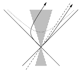
Figure 2: Generic evolution of the single-scalar, $k=0$, cosmologies as geodesics on the augmented target space. The plot shows the $\{\gamma,\varphi\}$-plane in the case of a positive exponential potential $V$ with constant characteristic functions satisfying $\alpha_{c}<a<\alpha_{h}$. The decelerating fixed point solution is shown as the dashed straight line outside the acceleration cone. Both generic geodesics start close to a null direction when the kinetic energy dominates and are attracted to the fixed point direction at late times. The geodesic on the left goes through a regime of transient acceleration when its tangent vector is steep enough to lie within the acceleration cone.

For $k\neq 0$, cosmological trajectories are no longer geodesics in the augmented target space but they are projections of geodesics in the doubly-augmented target space. The vector tangent to the geodesic corresponding to a $k\neq 0$ fixed point is

$$\partial_{\hat{t}}\Psi^{A}=\pm{1\over\sqrt{2}\Omega}\left(\sqrt{\left(d-1\right)}\,a,\ {\alpha_{c}\over a}\,\mathbf{a},\ \pm\sqrt{\left(d-1\right)}\,V_{0}^{-{1\over 2}}e^{\mathbf{a}\cdot{\bm{\phi}}+(d-3)\beta}\right)$$ (111)

where we have used (93) to get the last entry. Note that this is not a constant $(N+2)$-vector (even allowing for the fact that $a\varphi-\beta$ is constant at the fixed point) so the fixed point solution is not a straight line in the doubly-augmented target space, as was to be expected because its metric is neither flat nor conformally flat. However, using (111), and then (29), one finds that

$$\widetilde{G}_{AB}^{\rm acc}\,\partial_{\hat{t}}\Psi^{A}\partial_{\hat{t}}\Psi^{B}={1\over 2}\left[\alpha_{c}^{2}-a^{2}-k\,\alpha_{c}^{-2}|V|^{-1}e^{-2\beta}\right]=0\,.$$ (112)

This again confirms the zero acceleration of the $k\neq 0$ fixed point cosmologies.

6.3 Asymptotic Behaviour for Generic Potentials

The asymptotic (late-time) behaviour of a large class of cosmologies in models with rather general potentials can be determined by comparison with the asymptotic behaviour of cosmologies in models with exponential potentials. To demonstrate this, we discuss the case of flat cosmologies with positive potentials. In this case, the scalar fields must approach $\bm{\phi}\rightarrow\bm{\phi}_{0}$ at late times, where some components of the constant $N$-vector $\bm{\phi}_{0}$ may be infinite. The characteristic functions of the potential in this limit are also constant:

$$\mathbf{a}_{0}=\lim_{\bm{\phi}\rightarrow\bm{\phi}_{0}}\mathbf{a}(\bm{\phi})\,.$$ (113)

The absolute value $a_{0}=|\mathbf{a}_{0}|$ determines the late-time behaviour, by comparison with the critical and hypercritical exponents: if $a_{0}<\alpha_{c}$, then there will be late-time acceleration, with the trajectory approaching an approximate accelerating attractor; obvious examples are models for which $V$ has a strictly positive lower bound, so most models of interest will be those for which $V$ either tends to zero or has a minimum at zero. For $\alpha_{c}<a_{0}<\alpha_{h}$, there is late-time deceleration corresponding to the existence of an approximate late-time decelerating attractor. The asymptotic geodesics in both these cases are timelike. In contrast, for $a_{0}>\alpha_{h}$ the timelike geodesic asymptotes a null (and hence decelerating) trajectory.

To illustrate the above observations, we consider the following single-scalar examples.

• Inverse power law potentials:

  $$V=1/\varphi^{n}\,.$$ (114)

  These potentials have been much studied in quintessence models (see e.g. [1]). They also arise from dynamical breaking of supersymmetry [28]. With $\varphi_{0}=\infty$, one finds $a_{0}=0$. This implies late-time acceleration, even though the potential tends to zero at late-times.

• That any other value of $a_{0}$ may occur is illustrated by the potential

  $$V=\varphi^{2m}e^{-2a\varphi}\,,$$ (115)

  for which $a_{0}=a$ if we suppose that $\varphi\rightarrow\infty$ at late times. For such cosmologies the asymptotic behaviour is the same as it would be in the exponential potential model with dilaton coupling constant $a$.

• It may happen that at late times the scalar fields become trapped near a minimum of the potential. Near such a minimum, which we may assume to occur at the origin of field space, the potential takes the form

  $$V=\varphi^{2n}+\lambda$$ (116)

  for integer $n>0$. For positive $\lambda$ one finds

  $$a=-\frac{n\phi^{2n-1}}{\varphi^{2n}+\lambda}$$ (117)

  which tends to zero (i.e. $a_{0}=0$) as $\varphi\rightarrow 0$ for any $\lambda>0$. This implies late-time acceleration, due to the effective cosmological constant $\lambda$. However, we may now consider the limit $\lambda\rightarrow 0$, in which case $a_{0}=\infty>\alpha_{h}$, implying that the late-time trajectory is null, and hence decelerating.

7 Discussion

In this paper we have developed a geometrical method for the classification and visualisation of homogeneous isotropic cosmologies in multi-scalar models with an arbitrary scalar potential $V$. The method involves two steps. In the first step, the target space parametrised by the $N$ scalar fields is augmented to a larger $(N+1)$-dimensional space of Lorentzian signature, the logarithm of the scale factor playing the role of time. This is reminiscent of the role of the scale factor in mini-superspace models of quantum cosmology, especially if one views the scalar fields of our model as moduli-fields for extra dimensions. In this case, the Lorentzian metric on the augmented target space is the one induced from the Wheeler-DeWitt metric on the space of higher-dimensional metrics. This was the point of view adopted in [25], where it was also observed that when $V=0$ all flat ($k=0$) cosmologies are null geodesics in this metric (an observation that goes back to work of DeWitt on Kasner metrics [29]). When $V\neq 0$, flat cosmologies again correspond to trajectories in the augmented target space but they are neither null nor geodesic. However, as we have shown, all flat cosmologies are geodesics with respect to a conformally rescaled metric on the augmented target space, the conformal factor depending both on the scale factor and the potential. The conformal rescaling has no effect on null geodesics, of course, so flat cosmologies are still null geodesics whenever $V=0$, but now the trajectories of flat cosmologies are timelike geodesics when $V>0$ and spacelike geodesics when $V<0$. This is true not only for a potential of fixed sign but also for one that changes sign; in this case the tangent to the geodesic becomes null just as the scalar fields take values for which $V=0$.

The second step, which is needed for non-flat ($k=\pm 1$) cosmologies, is to further enlarge the target space to a ‘doubly-augmented’ target space foliated by copies of the augmented target space. One can choose the metric on this space, of signature $(1,N+1)$ for $k=-1$ and $(2,N)$ for $k=1$ and degenerate for $k=0$, such that geodesics yield (on projection) cosmological trajectories for any $k$ when projected onto a given hypersurface, and the geodesics are again timelike, null or spacelike according to whether $V$ is positive, zero or negative. This general construction thus includes all the previous ones as special cases.

Accelerating cosmologies have a simple interpretation in this new framework. Within the lightcone (defined by the metric with respect to which the trajectories are geodesics) there is an acceleration subcone. A given trajectory corresponds to an accelerating universe whenever its tangent vector lies within the acceleration cone. In particular, a flat cosmology undergoes acceleration whenever its geodesic trajectory bends into the acceleration cone within the lightcone of the augmented target space. This can happen only if the trajectory is timelike, which it will be if the potential is positive.

We have also presented in this paper a complete treatment (complementing many previous studies) of cosmological trajectories, for any $k$ and any spacetime dimension $d$, for the special case of simple exponential potentials. These potentials are characterised by a sign (the potential may be positive or negative) and a (dilaton) coupling constant $a$ (the magnitude of an $N$-vector coupling constant $\mathbf{a}$). As has long been appreciated [13], cosmological solutions in such models correspond, for an appropriate choice of time parameter, to trajectories of an autonomous dynamical system in a ‘phase space’ parametrised by the time-derivatives of the scale factor and scalar fields. The qualitative features of these trajectories (which should not be confused with trajectories in the ‘augmented target space’ parametrized by the fields themselves) are determined by the position and nature of any fixed points, which are of two types. There is always a $k=0$ fixed point unless $a=\alpha_{h}$ (the ‘hypercritical’ value of $a$ defined by this property) but it occurs only for $V>0$ if $a>\alpha_{h}$ and only for $V<0$ if $a>\alpha_{h}$. There is also a $k\neq 0$ fixed point if $V>0$, which coincides with the $k=0$ fixed point when $a=\alpha_{c}$, where $\alpha_{c}$ is the ‘critical’ value of $a$ (defined as the value at which fixed point cosmologies have zero acceleration).

These fixed point cosmologies have a very simple interpretation as trajectories in the augmented target space: they are straight lines. In the $k=0$ case these lines are also geodesics. For $V<0$ these geodesic lines lie outside the lightcone. For $V>0$ they lie inside the lightcone, but may lie either inside or outside the acceleration cone. For models obtained by (classical) compactification from a higher dimensional theory without a scalar field potential, the $k=0$ geodesic line always lies outside the acceleration cone, so only transient acceleration is possible in these models. For a single scalar field the transient acceleration is generic in the sense that it is a feature of all $k=0$ trajectories when $a>\alpha_{h}$ and of some when $a<\alpha_{h}$. In contrast, in the multi-scalar case, there are trajectories that correspond to eternally decelerating universes even when $a>\alpha_{h}$, so transient acceleration is less generic for more than one scalar field.

Although exponential potentials are of limited phenomenological value, they are important as ‘reference potentials’ in determining the asymptotic behaviour of cosmologies in models with other potentials, such as inverse power potentials. Essentially, any potential that falls to zero slower than the critical exponential potential (as do inverse power potentials) will lead to late-time eternal acceleration. Any potential that falls to zero faster than the hypercritical exponential potential will have a late-time behaviour that is approximately that of a model with zero potential.

Of course, there is no evidence for the existence of cosmological scalar fields, but there is evidence that the expansion of the universe is accelerating and hence for dark energy. Whatever produces this energy, it seems reasonable to suppose that it can be modeled by scalar fields. If so, it is possible that future observations may be interpreted as telling us something about the potential energy of these fields. In view of our current complete ignorance of what this potential might be, we have tried, as much as possible, to understand generic properties, and we hope that the methods developed here will be of further use in this respect.

Note added

The interpretation of solutions of gravitational theories as geodesics in a suitable metric space has a considerable history of which we were mostly unaware at the time of writing this paper. The geodesic interpretation of $k=0$ cosmologies that we have presented is closely related to the Maupertuis-Jacobi principle of classical mechanics. Relatively recent work on this topic includes [30, 31, 32]. A particle mechanics formulation of the geodesic interpretation described here, including our proposed extension to $k\neq 0$, has recently been found, and applied to a model in which cosmological singularities correspond to horizons in the augmented target space [33].

References

- [1] P.J.E. Peebles and B. Ratra. The cosmological constant and dark energy. Rev. Mod. Phys. 75 (2003) 559.
- [2] L. Cornalba and M. Costa. A new cosmological scenario in string theory. Phys. Rev. D66 (2002) 066001.
- [3] S. Kachru, R. Kallosh, A. Linde and S.P. Trivedi. De Sitter vacua in string theory. Phys. Rev. D68 (2003) 046005.
- [4] P.K. Townsend and M.N.R. Wohlfarth. Accelerating cosmologies from compactification. Phys. Rev. Lett. 91 (2003) 061302.
- [5] N. Ohta. Accelerating cosmologies from S-branes. Phys. Rev. Lett. 91 (2003) 061303.
- [6] S. Roy. Accelerating cosmologies from M/string theory compactifications. Phys. Lett. B567 (2003) 322.
- [7] M.N.R. Wohlfarth. Accelerating cosmologies and a phase transition in M-theory. Phys. Lett. B563 (2003) 1.
- [8] N. Ohta. A study of accelerating cosmologies from superstring/M-theories. Prog. Theor. Phys. 110 (2003) 269.
- [9] C.-M. Chen, P.-M. Ho, I.P. Neupane and J.E. Wang. A note on acceleration from product space compactification. J. High Energy Phys. 07 (2003) 017.
- [10] C.-M. Chen, P.-M. Ho, I.P. Neupane, N. Ohta and J.E. Wang. Hyperbolic space cosmologies. J. High Energy Phys. 10 (2003) 058.
- [11] M.N.R. Wohlfarth. Inflationary cosmologies from compactification? Phys. Rev. D69 (2004) 066002.
- [12] R. Emparan and J. Garriga. A note on accelerating cosmologies from compactifications and S-branes. J. High Energy Phys. 05 (2003) 028.
- [13] J.J. Halliwell. Scalar fields in cosmology with an exponential potential. Phys. Lett. B 185 (1987) 341.
- [14] L. Järv, T. Mohaupt and F. Saueressig. Quintessence cosmologies with a double exponential potential. hep-th/0403063.
- [15] A.B. Burd and J.D. Barrow. Inflationary models with exponential potentials. Nucl. Phys. B308 (1988) 929.
- [16] P.K. Townsend. Cosmic acceleration and M-theory. To appear in the proceedings of ICMP2003, Lisbon, Portugal, July 2003. hep-th/0308149.
- [17] I.P. Neupane. Accelerating cosmologies from exponential potentials. hep-th/0311071.
- [18] P.G. Vieira. Late-time cosmic dynamics from M-theory. Class. Quantum Grav. 21 (2004) 2421.
- [19] J.G. Russo. Exact solution of scalar-tensor cosmology with exponential potentials and transient acceleration. hep-th/0403010.
- [20] E.J. Copeland, A.R. Liddle and D. Wands. Exponential potentials and cosmological scaling solutions. Phys. Rev. D57 (1998) 4686.
- [21] I.P.C. Heard and D. Wands. Cosmology with positive and negative exponential potentials. Class. Quantum Grav. 19 (2002) 5435.
- [22] Z.K. Guo, Y.-S. Piao and Y.-Z. Zhang. Cosmological scaling solutions and multiple exponential potentials. Phys. Lett. B568 (2003) 1.
- [23] E. Bergshoeff, A. Collinucci, U. Gran, M. Nielsen and D. Roest. Transient quintessence from group manifold reductions or how all roads lead to Rome. Class. Quantum Grav. 21 (2004) 1947.
- [24] S. Tsujikawa, R. Brandenberger and F. Finelli. On the construction of nonsingular pre-big-bang and ekpyrotic cosmologies and the resulting density perturbations. Phys. Rev. D66 (2002) 083513.
- [25] G.W. Gibbons and P.K. Townsend. Cosmological evolution of degenerate vacua. Nucl. Phys. B282 (1987) 610.
- [26] T. Damour, M. Henneaux and H. Nicolai. Cosmological billiards. Class. Quantum Grav. 20 (2003) R145.
- [27] G.W. Gibbons, S.W. Hawking and J.M. Stewart. A natural measure on the set of all universes. Nucl. Phys. B281 (1987) 736.
- [28] I. Affleck, M. Dine and N. Seiberg. Dynamical supersymmetry breaking in supersymmetric QCD. Nucl. Phys. B241 (1984) 493.
- [29] B.S. DeWitt. Quantum theory of gravity II: the manifestly covariant theory. Phys. Rev. 162 (1967) 1195.
- [30] L. Smolin and C. Soo. The Chern-Simons invariant as the natural time variable for classical and quantum cosmology. Nucl. Phys. B449 (1995) 289.
- [31] J. Greensite. Field theory as free fall. Class. Quantum Grav. 13 (1996) 1339.
- [32] A. Carlini and J. Greensite. The mass shell of the universe. Phys. Rev. D55 (1997) 3514.
- [33] J.G. Russo and P.K. Townsend. Cosmology as relativistic particle mechanics: from big crunch to big bang. hep-th/0408220.