KUNS-1897 hep-th/0403031
Rolling Tachyon Solution
in Vacuum String Field Theory

We construct a time-dependent solution in vacuum string field theory and investigate whether the solution can be regarded as a rolling tachyon solution. First, compactifying one space direction on a circle of radius $R$, we construct a space-dependent solution given as an infinite number of $*$-products of a string field with center-of-mass momentum dependence of the form $e^{-bp^{2}/4}$. Our time-dependent solution is obtained by an inverse Wick rotation of the compactified space direction. We focus on one particular component field of the solution, which takes the form of the partition function of a Coulomb system on a circle with temperature $R^{2}$. Analyzing this component field both analytically and numerically using Monte Carlo simulation, we find that the parameter $b$ in the solution must be set equal to zero for the solution to approach a finite value in the large time limit $x^{0}\to\infty$. We also explore the possibility that the self-dual radius $R=\sqrt{\alpha^{\prime}}$ is a phase transition point of our Coulomb system.

1 Introduction

The rolling tachyon process represents the decay of unstable D-branes in bosonic and superstring theories [1, 2]. This process is described in the limit of vanishing string coupling constant by an exactly solvable boundary conformal field theory (BCFT). Study of this process has recently evolved into various interesting physics including open-closed duality at the tree level, a new understanding of $c=1$ matrix theory and Liouville field theory, and the rolling tachyon cosmology (see [3, 4, 5] and the references therein). However, there still remain many problems left unresolved; in particular, the closed string emission and its back-reaction [6].

One may think that such problems can be analyzed using string field theory (SFT), which is a candidate of nonperturbative formulation of string theory and has played critical roles in the study of static properties of tachyon condensation (see [7, 8] and the references therein). However, SFT has not been successfully applied to the time-dependent rolling tachyon process. The main reason is that no satisfactory classical solution representing the rolling process has been known in SFT, though there have appeared a number of approaches toward the construction of the solutions [9, 10, 11, 12, 13, 14, 15]. Among such approaches, refs. [9, 14] examined time-dependent solutions in cubic string field theory (CSFT) [16] by truncating the string field to a few lower mass component fields and expanding them in terms of the modes $e^{nx^{0}}$ ($n=0,\pm 1,\pm 2,\cdots$).

Let us summarize the result of our previous paper [14] (we use the unit of $\alpha^{\prime}=1$). We expanded the tachyon component field $t(x^{0})$ as

$$t(x^{0})=\sum_{n=0}^{\infty}t_{n}\cosh nx^{0}\,,$$ (1.1)

and solved the equation of motion for the coefficients $t_{n}$ numerically (by treating $t_{1}$ as a free parameter of the solution). Our analysis shows that the $n$-dependence of $t_{n}$ is given by

$$t_{n}\sim\lambda^{-n^{2}}\left(-\beta\right)^{n}\,,$$ (1.2)

up to a complicated subleading $n$-dependence. Here, $\lambda$ is a constant $3^{9/2}/2^{6}$ and $\beta$ is a parameter related to $t_{1}$. From the effective field theory analysis, the rolling tachyon solution is expected to approach the stable non-perturbative vacuum at large time $x^{0}\to\infty$ [17]. If $t_{n}$ behaves like (1.2), however, the profile of the tachyon field $t(x^{0})$ cannot be such a desirable one: it oscillates with rapidly growing amplitude (see also (3.1) and (3.2)):

$$t(x^{0})\sim e^{(x^{0})^{2}/(4\ln\lambda)}\times({\mbox{oscillating term}})\,.$$ (1.3)

Since the radius of convergence with respect to $x^{0}$ of the series (1.1) is infinite for $t_{n}$ of (1.2), we cannot expect that analytic continuation gives another $t(x^{0})$ which converges to a constant as $x^{0}\to\infty$.

In order for the series (1.1) to reproduce a desirable profile, it is absolutely necessary that the fast dumping factor $\lambda^{-n^{2}}$ of (1.2) disappears. If this were the case and, in addition, if $t_{n}$ were exactly given by

$$t_{n}=(-\beta)^{n}\,,$$ (1.4)

analytic continuation of the series (1.1) would lead to

$$t(x^{0})=-1+\frac{1}{1+\beta e^{x^{0}}}+\frac{1}{1+\beta e^{-x^{0}}}\,,$$ (1.5)

which approaches monotonically a constant as $x^{0}\to\infty$. This particular $t(x^{0})$ has another desirable feature that it becomes independent of $x^{0}$ when $\beta=0$ and $1$, which may correspond to sitting on the unstable vacuum and the stable one, respectively. Since CSFT should reproduce the rolling tachyon process, it is expected that the behavior (1.2) is an artifact of truncating the string field to lower mass component fields and that some kind of more sensible analysis would effectively realize $\lambda=1$.

The purpose of this paper is to study the rolling tachyon solution in vacuum string field theory (VSFT) [18, 19, 20, 21], which has been proposed as a candidate SFT expanded around the stable tachyon vacuum. The action of VSFT is simply given by that of CSFT with the BRST operator $Q_{\rm B}$ in the kinetic term replaced by another operator $\mathcal{Q}$ consisting only of ghost oscillators. Owing to the purely ghost nature of $\mathcal{Q}$, the classical equation of motion of VSFT is factorized into the matter part and the ghost one, each of which can be solved analytically to give static solutions representing D$p$-branes. In fact, analysis of the fluctuation modes around the solution has successfully reproduced the open string spectrum at the unstable vacuum although there still remain problems concerning the energy density of the solution [22, 23, 24]. If we can similarly construct time-dependent solutions in VSFT without truncation of the string field, we could study more reliably whether SFT can reproduce the rolling tachyon processes, and furthermore, the unresolved problems mentioned at the beginning of this section.

Our strategy of constructing a time-dependent solution in VSFT is as follows. First we prepare a lump solution depending on one space direction which is compactified on a circle of radius $R$. Then, we inverse-Wick-rotate this space direction to obtain a time-dependent solution following the BCFT approach [1]. The lump solution of VSFT localized in uncompactified directions has been constructed in the oscillator formalism by introducing the creation/annihilation operators for the zero-mode in this direction [19]. In the compactified case, however, we cannot directly apply this method. We instead construct the matter part $\Phi^{\rm m}$ of a lump solution as an infinite number of $*$-products of a string field $\Omega_{b}$; $\Phi^{\rm m}=\Omega_{b}*\Omega_{b}*\cdots*\Omega_{b}$ (the ghost part is the same as that in the static solutions). Since the equation of motion of $\Phi^{\rm m}$ is simply $\Phi^{\rm m}*\Phi^{\rm m}=\Phi^{\rm m}$, this gives a solution if the limit of an infinite number of $*$-product exists [27]. As the constituent $\Omega_{b}$, we adopt the one which is the oscillator vacuum with respect to the non-zero modes and has the Gaussian dependence $e^{-b\,p^{2}/4}$ on the zero-mode momentum $p$ in the compactified direction. Finally, our time-dependent solution is obtained by making the inverse Wick rotation of the compactified direction $X\to-iX^{0}$ or $-iX^{0}+\pi R$.

After constructing a time-dependent solution in VSFT, our next task is to examine whether it represents the rolling tachyon process. Our solution consists of an infinite number of string states, and we focus on one particular component field $t(x^{0})$ (we adopt the same symbol as the tachyon field in the CSFT analysis). This $t(x^{0})$ has the expansion (1.1) with $\cosh nx^{0}$ replaced by $\cosh(nx^{0}/R)$. What is interesting about $t(x^{0})$ is that it takes the form of the partition function of a statistical system of charges at sites distributed with an equal spacing on a unit circle. The temperature of this system is $R^{2}$. The charges interact through Coulomb potential and they also have a self energy depending on the parameter $b$ of $\Omega_{b}$. The partition function is obtained by summing over the integer value of the charge on each site keeping the condition that the total charge be equal to zero.

What we would like to know about $t(x^{0})$ are particularly the following two:

• Whether $t(x^{0})$ has a profile which converges to a constant as $x^{0}\to\infty$.

• Whether the critical radius $R=1$ in the BCFT approach [28, 29] is required also in our solution.

That we have to put $R=1$ in our solution is also natural in view of the fact that the correct value $-1$ of the tachyon mass squared is reproduced from the fluctuation analysis around the D25-brane solution of VSFT [22, 23, 24]. For these two problems, we carry out analysis using both analytic and numerical methods. In particular, we can apply the Monte Carlo simulation since $t(x^{0})$ is the partition function of a Coulomb system on a circle. We find that the coefficient $t_{n}$ of our VSFT solution has a similar $n$-dependence to (1.1) with $\lambda$ depending on the parameter $b$. This implies that the profile of $t(x^{0})$ is again an unwelcome one for a generic value of $b$: it is an oscillating function of $x^{0}$ with growing amplitude. However, we can realize $\lambda=1$ by putting $b=0$ and taking the number of $\Omega_{b}$ in $\Phi^{\rm m}=\Omega_{b}*\cdots*\Omega_{b}$ to infinity by keeping this number even. These properties seems to hold for any value of $R$. In order to see whether $R=1$ has a special meaning for our solution, we study the various thermodynamic properties of the Coulomb system $t(x^{0})$. First we argue using a naive free energy analysis that there could be a phase transition at temperature $R^{2}=1$. Below $R^{2}=1$ only the excitations of neutral boundstates of charges are allowed, but above $R^{2}=1$ excitations of isolated charges dominate the partition function. We carry out Monte Carlo study of the internal energy and the specific heat of the system, but cannot confirm the existence of this phase transition. However, we find that the correlation function of the charges show qualitatively different behaviors between the large and small $R^{2}$ regions when $b=0$, possibly supporting the existence of the phase transition.

The rest of this paper is organized as follows. In section 2, first briefly reviewing VSFT and its classical solutions representing various D$p$-branes, we construct time-dependent solutions following the strategy mentioned above. In section 3, we investigate the profile of the component field $t(x^{0})$ both analytically and numerically. In section 4, we argue that our solution with $b=0$ could give a rolling tachyon solution. In section 5, we study a possible phase transition at $R^{2}=1$ through various thermodynamic properties of the system. The final section (section 6) is devoted to a summary and discussions. In the appendix we present a proof concerning the minimum energy configuration of the Coulomb system.

2 Construction of a time-dependent solution in VSFT

In this section, we shall construct a time-dependent solution in VSFT. As stated in section 1, we first construct a lump solution which is localized in one spatial direction compactified on a circle of radius $R$. This solution is given as an infinite number of $\ast$-products of a string field $\Omega_{b}$; $\Omega_{b}*\Omega_{b}*\cdots*\Omega_{b}$. Our time-dependent solution is obtained by inverse-Wick-rotating the spatial direction to the time one. Throughout this paper, we use the convention $\alpha^{\prime}=1$.

2.1 D$p$-brane solutions in VSFT

In this subsection, we briefly review the construction of lump solutions in VSFT describing various D$p$-branes in the uncompactified space [19]. VSFT is a string field theory around the non-perturbative vacuum where there are only closed string states. Its action is written as follows using the open string field $\Psi$:

$$S =-\frac{1}{2}\Psi\cdot\mathcal{Q}\Psi-\frac{1}{3}\Psi\cdot(\Psi\ast\Psi)$$

$$=-\frac{1}{2}\,\langle\,\Psi\,|\,\mathcal{Q}\,|\,\Psi\,\rangle-\frac{1}{3}{}_{0}\langle\,\Psi\,|{}_{1}\langle\,\Psi\,|{}_{2}\langle\,\Psi\,|\,V_{3}\,\rangle_{012}.$$ (2.1)

The BRST operator $\mathcal{Q}$ of VSFT consists of only ghost operators, and it has no non-trivial cohomology. The three-string vertex $|\,V_{3}\,\rangle$ represents the mid-point interaction of three strings, and it factorizes into the direct product of the matter part and the ghost one. More generically, the matter part of the $N$-string vertex $|\,V_{N}\,\rangle$ representing the symmetric mid-point interaction of $N$-strings ($N=3,4,\cdots$) is given by [30, 31]

$$|\,V_{N}^{\rm m}\,\rangle_{01\cdots N-1}=\int\!d^{26}p_{0}\cdots\!\int\!d^{26}p_{N-1}\,\delta^{26}\!\biggl{(}\sum_{r=0}^{N-1}p_{r}\biggr{)}$$

$$\ \times\exp\!\left(\!-\eta_{\mu\nu}\sum_{r,s=0}^{N-1}\left[\frac{1}{2}\sum_{n,m=1}^{\infty}V_{nm}^{rs}a_{n}^{(r)\mu{\dagger}}a_{m}^{(s)\nu{\dagger}}+\sum_{n=1}^{\infty}V_{n0}^{rs}a_{n}^{(r)\mu{\dagger}}p_{s}^{\nu}+\frac{1}{2}V_{00}^{rs}p_{r}^{\mu}p_{s}^{\nu}\right]\right)\bigotimes_{r=0}^{N-1}|\,0;p_{r}\,\rangle_{r}\,,$$ (2.2)

where $|\,0;p_{r}\,\rangle$ is Fock vacuum of the $r$-th string carrying the center-of-mass momentum $p_{r}$ (the index $r$ specifying the $N$ strings runs from $0$ to $N-1$). Here we use the same convention as [18, 19, 20, 21]. $a_{n}^{\mu(r)}$ are the matter oscillators of non-zero modes normalized so that their commutation relations are

$$[a_{n}^{(r)\mu},a_{m}^{(s)\nu{\dagger}}]=\eta^{\mu\nu}\delta_{nm}\delta^{rs}\,,\quad(n,m\geq 1)\,.$$ (2.3)

The coefficients $V_{nm}^{rs}$ are called the Neumann coefficients. In particular, $V_{00}^{rs}$ is given by

$$V_{00}^{rs}=\begin{cases}\displaystyle-\ln\left|2\sin\frac{\pi(r-s)}{N}\right|\,,&(r\neq s)\,,\\[11.38109pt] \displaystyle 2\ln\!\left(\frac{N}{4}\right)\,,&(r=s)\,.\end{cases}$$ (2.4)

Note that $V_{nm}^{rs}$ depends on $N$ although we do not write it explicitly.

The action (2.1) leads to the equation of motion

$$\mathcal{Q}\Psi=-\Psi\ast\Psi\,.$$ (2.5)

Assuming that the solution is given as a product of the matter part and the ghost one, $\Psi=\Psi^{\rm m}\otimes\Psi^{\rm g}$, the equation of motion is reduced to

$$\Psi^{\rm m} =\Psi^{\rm m}\ast^{\rm m}\Psi^{\rm m}\,,$$ (2.6)

$$\mathcal{Q}\Psi^{\rm g} =-\Psi^{\rm g}\ast^{\rm g}\Psi^{\rm g}\,,$$ (2.7)

where $\ast^{\rm m}$ ($\ast^{\rm g}$) is the $*$-product in the matter (ghost) sector. In this paper, we assume that the ghost part $\Psi^{\rm g}$ is common to the various solutions, and focus on the matter part equation (2.6).

Classical solutions of (2.6) which represent the various D$p$-branes in spacetime are given in [19]. Let us review the two ways of constructing classical solutions representing the translationally invariant D25-brane. One way is to assume that $\Psi^{\rm m}$ is given in the form of a squeezed state, the exponential of an oscillator bilinear acting on the vacuum:

$$|\,\Psi^{\rm m}\,\rangle={\mathcal{N}}\exp\left(-\frac{1}{2}\eta_{\mu\nu}\sum_{m,n=1}^{\infty}S_{mn}a_{m}^{\mu{\dagger}}a_{n}^{\nu{\dagger}}\right)|\,0,0\,\rangle\,,$$ (2.8)

where $\mathcal{N}$ is a normalization factor. The equation of motion (2.6) is reduced to an algebraic equation for the infinite dimensional matrix $S_{mn}$, which, under a certain commutativity assumption and using the algebraic relations among the Neumann coefficients $V_{mn}^{rs}$ [30], can be solved to give $S_{mn}$ in terms of $V_{mn}^{rs}$ [32]:

$$S=CT,\qquad T=\frac{1}{2X}\left(1+X-\sqrt{(1+3X)(1-X)}\right)\,,$$ (2.9)

with the matrices $C$ and $X$ given by

$$C_{mn}=(-1)^{m}\delta_{mn},\qquad X=CV^{11}\,.$$ (2.10)

Another way is to construct $\Psi^{\rm m}$ as the sliver state [27]. Defining the wedge states as

$$|\,N\,\rangle_{0}=\underbrace{|\,0;0\,\rangle\ast|\,0;0\,\rangle\ast\cdots\ast|\,0;0\,\rangle}_{N-1}={}_{1}\langle\,0;0\,|{}_{2}\langle\,0;0\,|\cdots{}_{N-1}\langle\,0;0\,|\,V_{N}\,\rangle_{01\cdots N-1}\,,$$ (2.11)

they satisfy the following property:

$$|\,N\,\rangle\ast|\,M\,\rangle=|\,N+M-1\,\rangle\,.$$ (2.12)

Taking the limit $N,M\to\infty$, we have

$$|\,\infty\,\rangle\ast|\,\infty\,\rangle=|\,\infty\,\rangle\,.$$ (2.13)

Namely, the state $|\,\infty\,\rangle$ (sliver state) is a solution to (2.6). It has been proved that the two solutions, (2.8) and $|\,\infty\,\rangle$, are identical with each other [33].

Lump solutions localized in spatial directions can be constructed in the same way as the D25-brane solution. Let us denote the directions transverse to the brane by $x^{\alpha}$. In the squeezed state construction [19], we introduce the annihilation and the creation operators for the zero-mode in the transverse directions by

$$a_{0}^{\alpha}=\frac{\sqrt{b}}{2}\,\hat{p}^{\alpha}-\frac{i}{\sqrt{b}}\,\hat{x}^{\alpha}\,,\quad a_{0}^{\alpha{\dagger}}=\frac{\sqrt{b}}{2}\,\hat{p}^{\alpha}+\frac{i}{\sqrt{b}}\,\hat{x}^{\alpha}\,,$$ (2.14)

where $b$ is an arbitrary positive constant. Since the zero-modes $a_{0}^{\alpha}$ satisfy the same commutation relation (2.3) as the non-zero modes, we define the new Fock vacuum $|\,\Omega_{b}\,\rangle$ by

$$a_{n}^{(r)\alpha}|\,\Omega_{b}\,\rangle=0\,,\quad(n\geq 0)\,.$$ (2.15)

The new vacuum $|\,\Omega_{b}\,\rangle$ with the normalization $\langle\,\Omega_{b}\,|\,\Omega_{b}\,\rangle=1$ is expressed in terms of the momentum eigenstates as

$$|\,\Omega_{b}\,\rangle=\prod_{\alpha}\left(\frac{b}{2\pi}\right)^{1/4}\int_{-\infty}^{\infty}\!dp^{\alpha}\,e^{-(b/4)(p^{\alpha})^{2}}|\,0;p_{\alpha}\,\rangle\,.$$ (2.16)

With these oscillators and the coordinate-dependent vacuum $|\,\Omega_{b}\,\rangle$, the transverse part of the three-string vertex $|\,V_{3}\,\rangle$ can be written as

$$\exp\left(-\frac{1}{2}\sum_{r,s=0,1,2}\sum_{m,n=0}^{\infty}a^{(r)\alpha\dagger}_{m}V^{\prime rs}_{mn}a_{n}^{(s)\alpha\dagger}\right)|\,\Omega_{b}\,\rangle_{012}\,,$$ (2.17)

in terms of the new coefficients $V_{nm}^{\prime\,rs}$, which satisfy the same algebraic relations as $V_{nm}^{rs}$. Therefore, we can construct the D$p$-brane solutions just in the same way as the D25-brane solution:

$$|\,\Psi^{\rm m}_{p}\,\rangle =|\,\Psi^{\rm m}_{\parallel}\,\rangle\otimes|\,\Psi^{\rm m}_{\perp}\,\rangle$$

$$=\exp\biggr{(}-\frac{1}{2}\,\eta_{\mu\nu}\!\sum_{m,n=1}^{\infty}S_{mn}a^{\mu{\dagger}}_{m}a^{\nu{\dagger}}_{n}\biggr{)}|\,0;p\,\rangle\otimes\exp\biggr{(}-\frac{1}{2}\sum_{m,n=0}^{\infty}S^{\,\prime}_{mn}a^{\alpha{\dagger}}_{m}a^{\alpha{\dagger}}_{n}\biggr{)}|\,\Omega_{b}\,\rangle\,,$$ (2.18)

where the indices $\mu$, $\nu$ run the directions tangental to the branes ($\mu,\nu=0,1,\cdots,25-p$), and $S^{\prime}_{mn}$ is given by (2.9) with $V^{11}$ replaced by $V^{\prime 11}$. This lump solution contains one arbitrary parameter $b$, the physical meaning of which is not known. It has been shown that the ratio of the tensions of D$p$-brane solutions is independent of $b$ [34]. Later we will argue that we must choose $b=0$ to obtain a time-dependent solution with the desirable rolling profile.

Finally, note that, since the modified Neumann coefficients $V^{\prime\,rs}_{mn}$ satisfy the same algebra as the original $V^{rs}_{mn}$, the transverse part $|\,\Psi^{\rm m}_{\perp}\,\rangle$ of the lump solution (2.18) can be written as a sliver state:

$$|\,\Psi^{\rm m}_{\perp}\,\rangle=\lim_{N\rightarrow\infty}{}_{1}\langle\,\Omega_{b}\,|{}_{2}\langle\,\Omega_{b}\,|\cdots{}_{N-1}\langle\,\Omega_{b}\,|\,V_{N\,\perp}\,\rangle_{01\cdots N-1}\,,$$ (2.19)

where $|\,V_{N\,\perp}\,\rangle$ is the transverse part of the $N$-string vertex.

2.2 Time-dependent solution in VSFT

Now let us construct a time-dependent solution in VSFT which possibly represents the process of rolling tachyon. This consists of the following two steps:

• Construction of a lump solution of VSFT localized in one space direction which is compactified on a circle of radius $R$.

• Inverse Wick rotation of the compactified space direction to the time one on this lump solution to obtain a time-dependent solution in VSFT.

Since both the solution and the string vertices have factorized forms with respect to the spacetime directions, we shall focus only on this transverse direction of the brane in the rest of this paper.

First, we shall construct a lump solution on a circle. The squeezed state construction explained in the previous subsection, however, cannot be directly applied to the compactified case since the zero-mode creation/annihilation operators of (2.14) are ill-defined due to the periodicity $\hat{x}^{\alpha}\sim\hat{x}^{\alpha}+2\pi R$. Therefore, we shall adopt the sliver state construction of the lump solution. Namely, let us consider

$$\lim_{N\to\infty}\underbrace{|\,\Omega_{b}\,\rangle*\cdots*|\,\Omega_{b}\,\rangle}_{N-1}=\lim_{N\rightarrow\infty}{}_{1}\langle\,\Omega_{b}\,|\cdots{}_{N-1}\langle\,\Omega_{b}\,|\,V_{N}\,\rangle_{01\cdots N-1}\,,$$ (2.20)

with a suitably chosen $|\,\Omega_{b}\,\rangle$. If the limit $N\to\infty$ of (2.20) exits, it gives a solution of VSFT. Taking into account that the momentum zero-mode $p$ in the compactified direction takes discrete values $p=n/R$, we adopt as the state $|\,\Omega_{b}\,\rangle$ in (2.20) the following one which is a natural compactified version of (2.16):

$$|\,\Omega_{b}\,\rangle=\sum_{n=-\infty}^{\infty}e^{-(b/4)(n/R)^{2}}|\,0;n/R\,\rangle\,,$$ (2.21)

where $|\,0;n/R\,\rangle$ is the momentum eigenstate (and the Fock vacuum of the non-zero modes) with the normalization $\langle\,0;m/R\,|\,0;n/R\,\rangle=\delta_{n,m}$. The $N$-string vertex $|\,V_{N}^{\rm m}\,\rangle$ for the compactified direction is given by (2.2) with the replacements:

$$\int\!dp\rightarrow\frac{1}{R}\sum_{n}\,,\quad\delta(p)\rightarrow R\,\delta_{n,0}\,,\quad|\,0;p\,\rangle\rightarrow\sqrt{R}\,|\,0;n/R\,\rangle\,.$$ (2.22)

Then the state $|\,\Omega_{b}\,\rangle*\cdots*|\,\Omega_{b}\,\rangle$ in the $x$-representation for the center-of-mass dependence is given by

$$\langle\,x\,|\Bigl{(}\underbrace{|\,\Omega_{b}\,\rangle*\cdots*|\,\Omega_{b}\,\rangle}_{N-1}\Bigr{)}=\sum_{n_{0}=-\infty}^{\infty}\sum_{n_{1}=-\infty}^{\infty}\cdots\sum_{n_{N-1}=-\infty}^{\infty}\delta_{\sum_{r=0}^{N-1}n_{r},0}\exp\!\left(\frac{in_{0}x}{R}\right)$$

$$\times\exp\biggr{(}\!-\frac{1}{2}\sum_{n,m=1}^{\infty}V_{nm}^{00}a_{n}^{{\dagger}}a_{m}^{{\dagger}}-\sum_{s=0}^{N-1}\sum_{n=1}^{\infty}V_{n0}^{0s}a_{n}^{{\dagger}}\frac{n_{s}}{R}-\frac{1}{2R^{2}}\sum_{r,s=0}^{N-1}V_{00}^{rs}n_{r}n_{s}-\frac{b}{4R^{2}}\sum_{r=1}^{N-1}n_{r}^{2}\biggr{)}|\,0\,\rangle\,,$$ (2.23)

which in the limit $N\to\infty$ should give a lump solution on a circle. In this paper we are interested only in the time-dependence of the solution and hence ignore the overall constant factor multiplying the solution.

Our construction of a time-dependent solution of VSFT is completed by making the inverse Wick rotation $X\rightarrow-iX^{0}$, namely, $x\to-ix^{0}$ and $a_{n}^{\dagger}\to-ia_{n}^{\dagger}$, on this lump solution:

$$|\,\Psi(x^{0})\,\rangle=\lim_{N\to\infty}\sum_{n_{0}=-\infty}^{\infty}\sum_{n_{1}=-\infty}^{\infty}\cdots\sum_{n_{N-1}=-\infty}^{\infty}\delta_{\sum_{r=0}^{N-1}n_{r},0}\exp\!\left(\frac{n_{0}x^{0}}{R}\right)$$

$$\times\exp\biggr{(}\,\frac{1}{2}\sum_{n,m=1}^{\infty}V_{nm}^{00}a_{n}^{{\dagger}}a_{m}^{{\dagger}}+i\sum_{s=0}^{N-1}\sum_{n=1}^{\infty}V_{n0}^{0s}a_{n}^{{\dagger}}\frac{n_{s}}{R}-\frac{1}{2R^{2}}\sum_{r,s=0}^{N-1}Q_{rs}n_{r}n_{s}\biggr{)}|\,0\,\rangle\,,$$ (2.24)

where $Q_{rs}$ is defined by

$$Q_{rs}=V_{00}^{rs}+\frac{b}{2}\,\delta_{r,s}\left(\delta_{r,0}-1\right)=\begin{cases}\displaystyle-2\ln\!\left|2\sin\frac{\pi(r-s)}{N}\right|\,,&(r\neq s)\,,\\[12.0pt] \displaystyle 2\ln\!\left(\frac{N}{4}\right)+\frac{b}{2}\,,&(r=s\neq 0)\,,\\[10.0pt] \displaystyle 2\ln\!\left(\frac{N}{4}\right)\,,&(r=s=0)\,.\end{cases}$$ (2.25)

Taylor expansion of $\exp\left(i\sum_{s}\sum_{n}V_{n0}^{0s}a_{n}^{\dagger}n_{s}/R\right)$ in (2.24) gives an expression of $|\,\Psi(x^{0})\,\rangle$ as an infinite summation, $|\,\Psi(x^{0})\,\rangle=\sum_{\alpha}|\,\alpha\,\rangle\,\varphi_{\alpha}(x^{0})$, where $|\,\alpha\,\rangle$ are the static string states of the form $a^{\dagger}\cdots a^{\dagger}\exp(\frac{1}{2}\sum V_{mn}^{00}a^{\dagger}_{m}a^{\dagger}_{n})|\,0\,\rangle$, and $\varphi_{\alpha}(x^{0})$ are the corresponding time-dependent component fields. In this paper, we shall, for simplicity, focus on the component field of the pure squeezed state $\exp(\frac{1}{2}\sum V_{mn}^{00}a^{\dagger}_{m}a^{\dagger}_{n})|\,0\,\rangle$. Since we have $\lim_{N\to\infty}V_{mn}^{00}=S_{mn}$ [33], this component field is that for the state representing the unstable vacuum. Denoting this component field by $t(x^{0})$, we have

$$t(x^{0})=\sum_{n_{0}=-\infty}^{\infty}e^{n_{0}x^{0}/R}\,t_{n_{0}}\,,$$ (2.26)

where $t_{n_{0}}$ is given by

$$t_{n_{0}}=\sum_{\begin{smallmatrix}n_{1},\cdots,n_{N-1}=-\infty\\ (n_{0}+n_{1}+\cdots+n_{N-1}=0)\end{smallmatrix}}^{\infty}\exp\!\left(-\frac{1}{R^{2}}H(n_{r};n_{0})\right)\,,$$ (2.27)

with

$$H(n_{r};n_{0})=\frac{1}{2}\sum_{r,s=0}^{N-1}Q_{rs}n_{r}n_{s}\,.$$ (2.28)

Note that the coefficient $t_{n_{0}}$ can be regarded as the partition function of a statistical system with Hamiltonian $H$ and the temperature $R^{2}$.

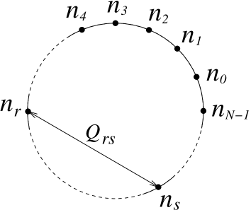
Figure 1: There are $N$ charges $n_{r}$ on the unit circle. Each charge $n_{r}$ takes integer values, and the total charge must be equal to zero. The charges $n_{r}$ and $n_{s}$ interact via the Coulomb potential $Q_{rs}$.

In this statistical system, we have $N$ charges $n_{r}$ on a unit circle at an equal interval (figure 1). The charges $n_{r}$ take integer values from $-\infty$ to $+\infty$, and they have the self interaction $Q_{rr}$ and the two-dimensional Coulomb interaction $Q_{rs}$ ($r\neq s$) between each other. In $t_{n_{0}}$, the charge $n_{0}$ at $r=0$ is fixed, and there is a constraint that the total charge be equal to zero. Note that $t_{n_{0}}$ is positive definite, $t_{n_{0}}>0$, and is even under $n_{0}\to-n_{0}$:

$$t_{-n_{0}}=t_{n_{0}}\,.$$ (2.29)

On the other hand, $t(x^{0})$ itself is interpreted as the partition function of the statistical system in the presence of the external source $x^{0}/R$ for $n_{0}$.

Solving the constraint $\sum_{r=0}^{N-1}n_{r}=0$ to eliminate $n_{N-1}$, $t_{n_{0}}$ and $t(x^{0})$ are rewritten using independent variables without constraint:

$$t_{n_{0}}=\sum_{n_{1},\cdots,n_{N-2}=-\infty}^{\infty}\exp\!\left(-\,\frac{1}{2R^{2}}\sum_{r,s=0}^{N-2}\widehat{Q}_{rs}n_{r}n_{s}\right)\,,$$ (2.30)

where $\widehat{Q}_{rs}$ is a $(N-1)\times(N-1)$ matrix given by

$$\widehat{Q}_{r,s}=Q_{rs}-Q_{r,N-1}-Q_{N-1,s}+Q_{N-1,N-1}\,,\quad(r,s=0,1,\cdots,N-2)\,.$$ (2.31)

We have checked numerically that the matrix $\widehat{Q}_{rs}$ is a positive definite matrix.

In addition to the above $|\,\Psi(x^{0})\,\rangle$ obtained by the inverse Wick rotation $X\rightarrow-iX^{0}$, we have another time-dependent solution via a different inverse Wick rotation, $X\rightarrow-iX^{0}+\pi R$. This new solution is obtained simply by inserting $(-1)^{n_{0}}$ into (2.24) and (2.26), and satisfies the hermiticity condition. As we shall explain in the next section, we expect that this new solution with $(-1)^{n_{0}}$ represents the rolling process to the stable tachyon vacuum, while the orignal solution given by (2.24) represents the rolling in the direction where the potential is unbounded from below.

3 Analysis of the component field $\boldsymbol{t(x^{0})}$

In this section, we study the profile of the component field $t(x^{0})$ given by (2.26) both analytically and numerically. If our VSFT solution (2.24) represents the rolling tachyon solution, the component field $t(x^{0})$ as well as the whole $|\,\Psi(x^{0})\,\rangle$ should approach zero, namely the tachyon vacuum, as $x^{0}\rightarrow\infty$.

Let us mention the expected $n_{0}$-dependence of the coefficient $t_{n_{0}}$, (2.27) and (2.30), necessary for $t(x^{0})$ to have a rolling tachyon profile. Suppose that the $n_{0}$-dependence of $t_{n_{0}}$ is given by

$$t_{n_{0}}=e^{-an_{0}^{2}}\,\widetilde{t}_{n_{0}}\,,$$ (3.1)

where $\widetilde{t}_{n_{0}}$ has a milder $n_{0}$-dependence than the leading factor $e^{-an_{0}^{2}}$. We expect that $\lim_{n\to\infty}\widetilde{t}_{n}/\widetilde{t}_{n+1}$ is finite and larger than one, namely, that the series (2.26) with $t_{n_{0}}$ replaced by $\widetilde{t}_{n_{0}}$ has a finite radius of convergence with respect to $x^{0}$. A typical example is $\widetilde{t}_{n_{0}}\sim e^{-b\left|n_{0}\right|}$. Such $t_{n_{0}}$ actually appeared in the time-dependent solution in CSFT in the level-truncation approximation [9, 14]. For this $t_{n_{0}}$, we have

$$t(x^{0})=e^{(x^{0})^{2}/(4a)}\,\widetilde{t}(x^{0}),\qquad\widetilde{t}(x^{0})=\sum_{n=-\infty}^{\infty}\widetilde{t}_{n}\,e^{-(x^{0}-2na)^{2}/(4a)}\,.$$ (3.2)

If $\widetilde{t}_{n_{0}}$ does not depend on $n_{0}$, $\widetilde{t}(x^{0})$ is a periodic function of $x^{0}$ with period $2a$, and the whole $t(x^{0})$ cannot have a desired profile: it oscillates with blowing up amplitude $e^{(x^{0})^{2}/(4a)}$ as $x^{0}\to\infty$. Even if $\widetilde{t}_{n_{0}}$ has a mild $n_{0}$-dependence such as $\widetilde{t}_{n_{0}}\sim e^{-b\left|n_{0}\right|}$, it seems very unlikely that $t(x^{0})$ approaches a finite value in the limit $x^{0}\to\infty$. These properties persist in the alternating sign solution $(-1)^{n_{0}}t_{n_{0}}$ obtained by another inverse Wick rotation mentioned at the end of section 2. Therefore, it is necessary that the leading term $e^{-an_{0}^{2}}$ in (3.1) is missing, namely, we must have $a=0$. If this is the case, the series $t(x^{0})$ (2.26) would have a finite radius of convergence, and the analytic continuation would give a globally defined $t(x^{0})$ such as (1.5). Since $t_{n_{0}}$ is positive definite, $t(x^{0})$ diverges at the radius of convergence and corresponds to the rolling in the direction of the unbounded potential. On the other hand, another $t(x^{0})$ with alternating sign coefficients $(-1)^{n_{0}}\,t_{n_{0}}$ is expected to be finite at the radius of convergence and represent the rolling to the tachyon vacuum.

In the rest of this section we shall study whether the condition $a=0$ is satisfied for the present solution. We shall omit the indices $0$ of $n_{0}$ and $x^{0}$ unless confusion occurs.

3.1 Analysis for $R^{2}\gg 1$ and $R^{2}\ll 1$

In this subsection, we shall consider the $n$-dependence of the coefficient $t_{n}$ of (2.30) for $R^{2}\gg 1$ and $R^{2}\ll 1$. First, for the analysis in the region $R^{2}\gg 1$ and also for later use, we present another expression of $t_{n}$ obtained by applying the Poisson’s resummation formula,

$$\sum_{n=-\infty}^{\infty}g(n)=\sum_{m=-\infty}^{\infty}\int_{-\infty}^{\infty}\!dy\,g(y)\,e^{2\pi imy}\,,$$ (3.3)

to the $n_{r}$-summations in (2.30):

$$t_{n} =R^{N-2}\Bigl{(}\det\widehat{\widehat{Q\,}}\Bigr{)}^{-1/2}\exp\!\left(-\frac{1}{2\bigl{(}\widehat{Q}^{-1}\bigr{)}_{00}}\frac{n^{2}}{R^{2}}\right)$$

$$\qquad\times\sum_{m_{1},\cdots,m_{N-2}=-\infty}^{\infty}\exp\left\{-2\pi^{2}R^{2}\sum_{r,s=1}^{N-2}m_{r}\Bigl{(}\widehat{\widehat{Q\,}}^{-1}\Bigr{)}_{rs}m_{s}+2\pi in\sum_{r=1}^{N-2}n_{r}^{C}m_{r}\right\}\,,$$ (3.4)

where the matrix $\widehat{\widehat{Q\,}}$ is the lower-right $(N-2)\times(N-2)$ part of $\widehat{Q}$,

$$\widehat{\widehat{Q\,}}_{rs}=\widehat{Q}_{rs}\,,\quad(r,s=1,2,\cdots,N-2)\,,$$ (3.5)

and $n_{r}^{C}$ is defined by

$$n_{r}^{C}=-\sum_{s=1}^{N-2}\bigl{(}\widehat{\widehat{Q\,}}^{-1}\bigr{)}_{rs}\widehat{Q}_{s0}\,,\quad(r=1,2,\cdots,N-2)\,.$$ (3.6)

In obtaining the expression (3.4), we have used that

$$\widehat{Q}_{00}-\sum_{r,s=1}^{N-2}\widehat{Q}_{0r}\bigl{(}\widehat{\widehat{Q\,}}^{-1}\bigr{)}_{rs}\widehat{Q}_{s0}=\frac{1}{\bigl{(}\widehat{Q}^{-1}\bigr{)}_{00}}\,,$$ (3.7)

which is valid for any matrix $\widehat{Q}$ and its $(N-2)\times(N-2)$ submatrix $\widehat{\widehat{Q\,}}$.

Some comments on the formula (3.4) are in order. First, $\{n_{r}^{C}\}$ in (3.6) is nothing but the configuration which, without the constraint that $n_{r}^{C}$ be integers and keeping $n=1$ fixed, minimizes the Hamiltonian (2.28),

$$H(n_{r};n)=\frac{1}{2}\sum_{r,s=1}^{N-2}\widehat{\widehat{Q\,}}_{rs}n_{r}n_{s}+n\sum_{r=1}^{N-2}\widehat{Q}_{0r}n_{r}+\frac{1}{2}\,\widehat{Q}_{00}n^{2}\,.$$ (3.8)

Figure 2: The minimum energy non-integer configurations $\{n_{r}^{C}\}$ with $n=1$ in the case $N=100$. The value of $b$ is $b=0.1$ in the left figure and $b=10$ in the right one.

Figure 2 shows the configurations $\{n_{r}^{C}\}$ in the cases of $b=0.1$ (left figure) and $b=10$ (right figure) for $N=100$. As seen from the figure, $\{n_{r}^{C}\}$ is localized around $r=0\pmod{N}$ to screen the charge $n=1$.

Our second comment is on the term $\exp\bigl{(}-\bigl{[}2\bigl{(}\widehat{Q}^{-1}\bigr{)}_{00}\bigr{]}^{-1}\left(n^{2}/R^{2}\right)\bigr{)}$ in (3.4). The exponent is equal to the value of the Hamiltonian $H$ for the configuration $\{n\cdot n_{r}^{C}\}$, namely, the (non-integer) configuration minimizing $H$ for a given $n$:

$$H(n\cdot n_{r}^{C}\,;n)=\frac{n^{2}}{2\bigl{(}\widehat{Q}^{-1}\bigr{)}_{00}}\,.$$ (3.9)

As was analyzed in [19], $1/\bigl{(}\widehat{Q}^{-1}\bigr{)}_{00}$ is finite in the limit $N\to\infty$.

Figure 3: $\lim_{N\to\infty}\bigl{[}2\bigl{(}\widehat{Q}^{-1}\bigr{)}_{00}\bigr{]}^{-1}$ as a function $\ln b$. The dots represent $\lim_{N\to\infty}\bigl{[}2\bigl{(}\widehat{Q}^{-1}\bigr{)}_{00}\bigr{]}^{-1}$ at $b=1/100$, $1/10$, $1$, $10$, $100$, $1000$ obtained by evaluating its values for $N=50$, $100$, $200$, $300$, $400$, $500$, $600$ and then extrapolating them to $N=\infty$ by using the fitting function of the form $\sum_{k=0}^{3}c_{k}/N^{k}$. The curve interpolating these six points is $0.429214+0.216204\times\ln b+0.0379729\times(\ln b)^{2}+0.00186225\times(\ln b)^{3}$.

Figure 3 shows $\lim_{N\to\infty}\bigl{[}2\bigl{(}\widehat{Q}^{-1}\bigr{)}_{00}\bigr{]}^{-1}$ as a function of $\ln b$. It is a monotonically increasing function of $b$ and, as we shall see in section 4, approaches zero as $b\to 0$.

Now let us consider $t_{n}$ for $R^{2}\gg 1$. Since $\widehat{\widehat{Q\,}}$ is a positive definite matrix, the configuration $m_{r}=0$ for all $r=1,2,\cdots,N-2$ dominates the $m_{r}$-summation in (3.4) for $R^{2}\gg 1$. Namely, we have

$$t_{n}\simeq R^{N-2}\Bigl{(}\det\widehat{\widehat{Q\,}}\Bigr{)}^{-1/2}\exp\!\left(-\frac{1}{2\bigl{(}\widehat{Q}^{-1}\bigr{)}_{00}}\frac{n^{2}}{R^{2}}\right)\,,\quad(R^{2}\gg 1)\,.$$ (3.10)

This expression can also be obtained by simply replacing the $n_{r}$-summations in (2.30) with integrations over continuous variables $p_{r}=n_{r}/R$. Since the coefficient of $n^{2}$ in the exponent is non-vanishing for $b>0$, this $t_{n}$ cannot lead to a desirable rolling profile.

On the other hand, $t_{n}$ (2.30) for $R^{2}\ll 1$ can be approximated by

$$t_{n}\simeq\exp\!\left(-\frac{1}{R^{2}}H\!\left(n_{r}^{I}(n);n\right)\right)\,,\quad(R^{2}\ll 1)\,,$$ (3.11)

where $\{n_{r}^{I}(n)\}$ is the integer configuration which minimizes the Hamiltonian for a given $n$. This configuration $\{n_{r}^{I}(n)\}$ is in general different from but is close to $\{n\cdot n_{r}^{C}\}$, the configuration minimizing $H(n_{r};n)$ without the integer restriction. Therefore, rewriting (3.11) as

$$t_{n}\simeq\exp\!\left(-\frac{1}{2\bigl{(}\widehat{Q}^{-1}\bigr{)}_{00}}\frac{n^{2}}{R^{2}}\right)\times\exp\!\left(-\frac{1}{R^{2}}\,\Delta H(n)\right)\,,$$ (3.12)

with $\Delta H(n)$ defined by

$$\Delta H(n)=H\!\left(n_{r}^{I}(n);n\right)-H\!\left(n\cdot n_{r}^{C};n\right)\,,$$ (3.13)

the second factor of (3.12) is expected to have a milder $n$-dependence than the first one. Figure 4 shows $\Delta H(n)$ for $N=2048$ and $b=0.1$. We see that $\Delta H(n)$ is in fact roughly proportional to $n$.

Figure 4: $\Delta H(n)$ v.s. $n$ for $N=2048$ and $b=0.1$. For obtaining $\Delta H(n)$, we approximate the integer-valued charge $n_{r}^{\rm I}(n)$ by the integer nearest to $n\cdot n_{r}^{\rm C}$. However, this $\{n_{r}^{\rm I}(n)\}$ does not necessarily satisfy the constraint $n+\sum_{r=1}^{N-1}n_{r}^{\rm I}(n)=0$. In the figure, only the points which satisfy the constraint are plotted. Distribution of the points is insensitive to the value of $N$ if it is large enough.

Therefore, we cannot obtain a rolling profile in the case $R^{2}\ll 1$ either.

Summarizing this subsection, for both $R^{2}\gg 1$ and $R^{2}\ll 1$, the coefficient $t_{n}$ of the component field $t(x)$ has the leading $n$-dependence of the form

$$t_{n}\sim\exp\left(-\frac{1}{2(\widehat{Q}^{-1})_{00}}\,\frac{n^{2}}{R^{2}}\,\right)\,.$$ (3.14)

Then, $t(x)$ itself shows the behavior

$$t(x) \sim\exp\left(\frac{1}{2}(\widehat{Q}^{-1})_{00}(x)^{2}\right)\times({\mbox{oscillating part}})\,,$$ (3.15)

and cannot approach the tachyon vacuum as $x\to\infty$. This is the case even if we adopt the alternating sign solution $(-1)^{n}t_{n}$.

3.2 Numerical analysis using Monte Carlo simulation

For studying $t_{n}$ and $t(x)$ for intermediate values of $R^{2}$, we shall carry out Monte Carlo simulation of the Coulomb system with partition function (2.27), Hamiltonian $H$ and temperature $R^{2}$. We have adopted the Metropolis algorithm. Since the total charge must be kept zero, a new configuration is generated from the old one $\{n_{r}\}$ by randomly choosing two points $r$ and $s$ on the circle and making the change $(n_{r},n_{s})\to(n_{r}+1,n_{s}-1)$. This new configuration is accepted/rejected according to the standard Metropolis algorithm.

3.2.1 Time derivatives of $\boldsymbol{\ln t(x)}$

First we investigate the time derivatives of the logarithm of $t(x)$. Defining $T(x)$ by

$$t(x)=e^{T(x)}\,,$$ (3.16)

we have

$$\frac{dT(x)}{dx} =\frac{1}{R}\,\langle n\rangle_{x}\,,$$ (3.17)

$$\frac{d^{2}T(x)}{d{x}^{2}} =\frac{1}{R^{2}}\left(\langle n^{2}\rangle_{x}-\langle n\rangle_{x}^{2}\right)\,,$$ (3.18)

where the average $\langle\mathcal{O}\rangle_{x}$ for a given $x$ is defined by

$$\langle\mathcal{O}\rangle_{x}=\frac{1}{t(x)}\sum_{\begin{smallmatrix}n,n_{1},\cdots,n_{N-1}=-\infty\\ \left(n+\sum_{r=1}^{N-1}n_{r}=0\right)\end{smallmatrix}}^{\infty}\!\!\mathcal{O}\,e^{-H(n_{r};n)/R^{2}+nx/R}\,.$$ (3.19)

Figure 5: The numerical results of $dT(x)/dx$ at $x=0.5,1.0,1.5,\cdots,50.0$. Here we have taken $b=10$, $R^{2}=1$ and $N=256$. These points are well fitted by a linear function $0.4530x-0.1713$, and the slope $0.4530$ is close to $(\hat{Q}^{-1})_{00}=0.4497$ for the present $b$ and $N$. The small oscillatory behavior can be better observed in $d^{2}T(x)/dx^{2}$ shown in figure 6.

$R^{2}$	0.3	0.5	1.0	1.5	2.0	3.0	5.0	$(\widehat{Q}^{-1})_{00}$
slope	$0.4557$	$0.4540$	$0.4530$	$0.4502$	$0.4498$	$0.4498$	$0.4497$	$0.4497$

Table 1: The slope of the linear function of $x$ obtained by fitting the Monte Carlo results of $\langle n\rangle_{x}/R$ with $b=10$ and $N=256$. They are almost independent of $R^{2}$ and close to $(\widehat{Q}^{-1})_{00}$.

The numerical results of the “velocity” (3.17) versus $x$ for $b=10$, $R^{2}=1$ and $N=256$ are shown in figure 5. We find that $dT(x)/dx$ is almost linear in $x$. The slope of the fitted linear function for the various $R^{2}$ and $b=10$ and $N=256$ as well as the value of $(\widehat{Q}^{-1})_{00}$ for the present $b$ and $N$ are shown in table 1. These results show that the behavior of (3.15) obtained in the regions $R^{2}\ll 1$ and $R^{2}\gg 1$ is valid also in the intermediate region of $R^{2}$.

Figure 6: $d^{2}T(x)/dx^{2}$ at $x=0.5,1.0,1.5,\cdots,50.0$. Here we have taken $b=10$, $R^{2}=1$ and $N=256$. The horizontal line shows the value of $(\widehat{Q}^{-1})_{00}=0.4497$ for the present $b$ and $N$.

The Monte Carlo results of the “acceleration” (3.18) at various $x$ are shown in figure 6 in the case of $b=10$, $R^{2}=1$ and $N=256$. The acceleration oscillates with period roughly equal to $8$. The center of the oscillation is around $(\widehat{Q}^{-1})_{00}=0.4497$, which is consistent with (3.15). We have studied the acceleration for other values of $R^{2}$ and found that it oscillates around $(\widehat{Q}^{-1})_{00}$ for any $R^{2}$.

3.2.2 Numerical analysis of $\boldsymbol{t_{n}}$

The $n$-dependence of $t_{n}$ itself can be directly measured using Monte Carlo simulation as follows [35]. Here, we use instead of $R^{2}$ the inverse temperature $\beta=1/R^{2}$, and make explicit the $\beta$-dependence of $t_{n}$ to write it as $t_{n,\beta}$. Let us define the average $\langle\mathcal{O}\rangle_{n,\beta}$ with subscript $n$ and $\beta$ by

$$\langle\mathcal{O}\rangle_{n,\beta}=\frac{1}{t_{n,\beta}}\sum_{\begin{smallmatrix}n_{1},\cdots,n_{N-1}=-\infty\\ \left(n+\sum_{r=1}^{N-1}n_{r}=0\right)\end{smallmatrix}}^{\infty}\mathcal{O}\,e^{-\beta H(n_{r};n)}\,.$$ (3.20)

Integrating the relation

$$\frac{\partial}{\partial\beta}\ln t_{n,\beta}=\langle-H\,\rangle_{n,\beta}\,,$$ (3.21)

with respect to $\beta$, we obtain

$$\frac{t_{n,\beta}}{t_{n,\beta=0}}=\exp\left(\int_{0}^{\beta}d\beta^{\prime}\langle-H\,\rangle_{n,\beta^{\prime}}\right)\,,$$ (3.22)

and hence

$$\frac{t_{n,\beta}}{t_{n=0,\beta}}=\frac{t_{n,\beta=0}}{t_{n=0,\beta=0}}\exp\left(\int_{0}^{\beta}d\beta^{\prime}\left(\langle-H\,\rangle_{n,\beta^{\prime}}-\langle-H\,\rangle_{n=0,\beta^{\prime}}\right)\right)\,.$$ (3.23)

Eq. (3.10) implies that $t_{n,\beta=0}$ is independent of $n$ and therefore $t_{n,\beta=0}/t_{n=0,\beta=0}=1$. Thus, we obtain the formula

$$\frac{t_{n,\beta}}{t_{n=0,\beta}}=\exp\left(-\int_{0}^{\beta}d\beta^{\prime}\bigr{(}\langle H\rangle_{n,\beta^{\prime}}-\langle H\rangle_{n=0,\beta^{\prime}}\bigr{)}\right)\,.$$ (3.24)

This allows us, in principle, to directly evaluate the $n$-dependence of $t_{n}$ using the expectation values of $H$ obtained by Monte Carlo simulation. Note that $\langle H\rangle_{n,\beta}$ in high temperature region $\beta\ll 1$ is given using (3.10) by

$$\langle H\rangle_{n,\beta}\simeq\frac{N-2}{2\beta}+\frac{1}{2(\widehat{Q}^{-1})_{00}}\cdot n^{2}\,,\quad(\beta\ll 1)\,.$$ (3.25)

Figure 7: $\langle H\rangle_{n,\beta}-\langle H\rangle_{n=0,\beta}-n^{2}/(2(\widehat{Q}^{-1})_{00})$ for $n=10$ (red points), $n=20$ (green), $n=40$ (blue), and $n=100$ (purple). Here we have taken $N=256$ and $b=10$.

Figure 7 shows the Monte Carlo result of $\langle H\rangle_{n,\beta}-\langle H\rangle_{n=0,\beta}-n^{2}/(2(\widehat{Q}^{-1})_{00})$, namely, the deviation of $\langle H\rangle_{n,\beta}-\langle H\rangle_{n=0,\beta}$ from the high temperature value, for the various values of $n$ ($b=10$ and $N=256$). As $\beta$ is decreased, the data for each $n$ approach zero. On the other hand, they seem to approach a positive constant as $\beta$ is increased. Since the asymptotic value at large $\beta$ grows no faster than linearly in $n$, the results of figure 7 together with the formula (3.24) seems consistent with our low temperature analysis using (3.12) and figure 4.

From our analyses in this subsection we have found that the behaviors (3.14) of $t_{n}$ and (3.15) of $t(x)$ in the $R^{2}\gg 1$ and $R^{2}\ll 1$ regions are valid for any $R^{2}$. Concerning these behaviors, $R=1$ does not seem to be a special radius.

4 Possible rolling solution with $\boldsymbol{b=0}$

Our analysis in the previous section implies that rolling solutions with desirable profile can never be obtained unless the coefficient of $n^{2}$ in the exponent of (3.14) vanishes. Namely, we must have

$$\frac{1}{(\widehat{Q}^{-1})_{00}}=0\,.$$ (4.1)

This condition can in fact be realized by putting $b=0$ as can be inferred from figure 3, though the precise way how this condition is satisfied differs between the $N=\mbox{even}$ and the odd cases. For an even (and finite) $N$, the condition (4.1) is satisfied by simply putting $b=0$. This is because $\widehat{Q}$ with $N=\mbox{even}$ and $b=0$ has a zero-mode $\{(-1)^{r}\}$:

$$\sum_{s=0}^{N-2}\widehat{Q}_{rs}(-1)^{s}=0\,,\quad(r=0,1,\cdots,N-2;\,N=\mbox{even},b=0)\,.$$ (4.2)

This zero-mode is at the same time the minimum energy configuration $n_{r}^{C}$ (3.6).

On the other hand, in the $N=\mbox{odd}$ case, the condition (4.1) is realized by putting $b=0$ and in addition taking the limit $N\to\infty$. In fact, numerical analysis shows that

$$\frac{1}{(\widehat{Q}^{-1})_{00}\bigr{|}_{b=0}}=\frac{1.705}{N}+O\!\left(\frac{1}{N^{2}}\right)\,,\quad(N\gg 1,N=\mbox{odd})\,.$$ (4.3)

This property is related to the fact that the matrix $\widehat{Q}$ with $b=0$ has an approximate zero-mode for large and odd $N$. This approximate zero-mode, which is at the same time the minimum energy configuration $n_{r}^{C}$ (3.6), is given by

$$n_{r}^{C}\simeq(-1)^{r}\times\left(1-\frac{2\left|r\right|}{N+1}\right)\,,\quad\left(r=0,\pm 1,\pm 2,\cdots,\pm(N-1)/2\right)\,,$$ (4.4)

where the index $r$ should be understood to be defined $\mbox{mod}\,N$; $n_{r}=n_{r+N}$. This configuration satisfies $\sum_{r=0}^{N-1}n_{r}^{C}=0$ and

$$\sum_{s=0}^{N-2}\widehat{Q}_{rs}n_{s}^{C}=O\!\left(\frac{1}{N}\right)\,,\quad(r=0,1,\cdots,N-2;\,N\gg 1,b=0)\,.$$ (4.5)

A proof of (4.5) is given in the appendix.

In the rest of this section we shall consider only the case of $N=\mbox{odd}$ since (2.12) is closed among the $|\,N=\mbox{odd}\,\rangle$ states ($|\,N\,\rangle$ is the state given by (2.20) in the present case). Here we shall just make a comment on the case of $N=\mbox{even}$. When $N=\mbox{even}$ and $b=0$, the coefficient $t_{n}$ is independent of $n$ as can be seen from the expression (3.4) with $n_{r}^{C}=(-1)^{r}$. Therefore, we have $t(x)=t_{0}\sum_{n=-\infty}^{\infty}(\pm 1)^{n}e^{nx/R}$. A naive summation of this series gives $t(x)=0$, or the Poisson’s resummation formula gives $t(x)=2\pi t_{0}\sum_{m={\rm even}/{\rm odd}}\delta\left(ix/R-\pi m\right)$ [36].

We would like to investigate whether the solution with $b=0$ and $N(={\rm odd})\to\infty$ can be regarded as a rolling solution. However, it is not an easy matter to repeat the Monte Carlo analysis of Sections 3.2.1 and 3.2.2 in the present case. First, since the coefficient $(\widehat{Q}^{-1})_{00}$ of the leading $x$-dependent term of (3.15) blows up as $N\to\infty$, so do the slope of the velocity curve of figure 5 and the central value of the acceleration curve of figure 6. Therefore, it is hard to read off the subleading $x$-dependence which should become the leading one in the limit $N\to\infty$. Second, the direct evaluation of the coefficient $t_{n}$ using the formula (3.24) is not an easy task because of bad statistics problem. Namely, the difference $\langle H\rangle_{n,\beta}-\langle H\rangle_{n=0,\beta}$, which is of order $n^{2}/(2(\widehat{Q}^{-1})_{00})$ (see (3.25)), is very small compared with the leading bulk term $(N-2)/(2\beta)$ of $\langle H\rangle$ when $b=0$.

Here we shall content ourselves with the analysis of $t_{n}$ in the low temperature region $R^{2}\ll 1$ using the expression (3.12). Since the leading term $\exp\bigl{(}-n^{2}/(2(\widehat{Q}^{-1})_{00}R^{2})\bigr{)}$ of (3.12) disappears in the limit $N\to\infty$, we study the $n$-dependence of $\Delta H(n)$ in the same way as we did in figure 4. The result for $N=8191$ is plotted in figure 8.

Figure 8: $\Delta H(n)$ v.s. $n$ for $N=8191$ and $b=0$.

Note that the data of figure 8 has an approximate periodic structure with respect to $n$ with period of about $4100$. This periodicity can be understood from (3.4) for $t_{n}$ and the expression (4.4) for $n_{r}^{C}$ independently of the low temperature approximation. In fact, (3.4) without the leading term $\exp\bigl{(}-n^{2}/(2(\widehat{Q}^{-1})_{00}R^{2})\bigr{)}$ is invariant under the shift $n\to n+(N+1)/2$ since the change of the exponent in the $m_{r}$-summations under this shift is an integer multiple of $2\pi i$ for $n_{r}^{C}$ of (4.4). Although figure 8 shows data only for positive values of $n$, recall that $t_{n}$ is even under $n\to-n$; (2.29). This parity symmetry and the periodicity lead to the structure shown in figure 8.

The periodicity stated above,

$$t_{n+(N+1)/2}=t_{n}\,,$$ (4.6)

is not an exact one for a finite $N$ since both the condition (4.1) and eq. (4.4) for $n_{r}^{C}$ are only approximately satisfied. If the periodicity (4.6) were exact, $t(x)$ given by (2.26) could be rewritten as

$$t(x)=t_{\mbox{\scriptsize one-period}}(x)\sum_{k=-\infty}^{\infty}\exp\!\left(\frac{N+1}{2R}\,kx\right)\,,$$ (4.7)

where $t_{\mbox{\scriptsize one-period}}(x)$ is defined by

$$t_{\mbox{\scriptsize one-period}}(x)=\sum_{n=-[N/4]}^{[(N+1)/4]}t_{n}\,e^{nx/R}\,,$$ (4.8)

with $[c]$ being the largest integer not exceeding $c$. Namely, $t_{\mbox{\scriptsize one-period}}(x)$ is the one period part around $n=0$ in the summation of $t(x)$. The geometric series multiplying (4.7) is formally summed up to give an unwelcome result; it is equal to zero or the summation of delta functions for pure imaginary values of $x$. However, since the periodicity (4.6) is not exact for a finite $N$, we have to carry out more precise analysis taking into account the violation of the periodicity to obtain the profile $t(x)$ in the limit $N\to\infty$. Here we would like to propose another way of defining $t(x)$ which could lead to a desirable rolling profile. It is the $N\to\infty$ limit of the one period summation (4.8):

$$t(x)=\lim_{N\to\infty}t_{\mbox{\scriptsize one-period}}(x)\,.$$ (4.9)

This is also formally equal to the original summation (2.26) with $N=\infty$.

Let us return to the low temperature analysis with $R^{2}\ll 1$. For $t(x)$ given by (4.9), it is sufficient to study the $n$-dependence of $\Delta H(n)$ only in the half period region $n\in\bigl{[}0,[(N+1)/4]\bigr{]}$, which is shown in figure 9 for $N=8191$.

Figure 9: $\Delta H(n)$ for $n\in[0,2048]$ in the case $N=8191$. The red line is an auxiliary one with slope 3/2.

As shown in figure 9, $\Delta H(n)$ has a complicated structure with peaks and valleys. However, if we neglect such local structures and see figure 9 globally, we find that $\Delta H(n)$ grows almost linearly in $n$; $\Delta H(n)\propto n$ (the red line in figure 9 is the line with slope $3/2$). This could give a desirable $t_{n}$ with the behavior (1.4) up to complicated local structures. However, it is a nontrivial problem whether the $N\to\infty$ limit of (4.9) really exists even when we take into account the local structures. Here we shall point out a kind of self-similarity of $\Delta H(n)$ and hence of $t_{n}$; $2\,\Delta H(n)|_{N}\simeq\Delta H(2n)|_{2N}$.

Figure 10: $\Delta H(n)$ for $N=8191$ (blue points) and that for $N=4095$ (red points). Both the horizontal and the vertical scales are doubled for the red points.

Figure 10 shows $\Delta H(n)$ for $N=8191$ (blue points) and that for $N=4095$ (red points). Both the horizontal and the vertical scales are doubled for the $N=4095$ points. For example, the real coordinate of the red point $(1500,1600)$ in the figure is actually $(750,800)$. Note that the red points and the blue ones have overlapping local structures. It is our future subject to study whether $t(x)$ of (4.9) can exist for $t_{n}$ with such self-similarity.

5 Thermodynamic properties of $\boldsymbol{t(x)}$

In the BCFT analysis, the rolling tachyon solution is obtained by the inverse Wick rotation of one space direction compactified on a circle at the self dual radius $R=1$ [28, 1]. Therefore, also in our VSFT construction of the rolling tachyon solution, it is natural to expect that the meaningful solution exists only at $R=1$. This is also supported by the fact that the correct tachyon mass squared $-1$ has been successfully reproduced in the analysis of the fluctuation modes around the D25-brane solution in VSFT [22, 23, 24]. If the tachyon mass squared is equal to $-1$, the natural mode of the expansion in (2.26) is $e^{nx}$ with $R=1$ [9, 14]; in particular, the $n=\pm 1$ modes $e^{\pm x}$ are the massless modes at the unstable vacuum.

In this section we shall study how this critical radius $R=1$ appears in our construction of time-dependent solution in VSFT, especially in the component field $t(x)$. One would naively expect that the $N\to\infty$ limit of our solution (2.24) can exist only at $R=1$. Here, we do not pursue this possibility directly, but instead address the problem from a statistical mechanics point of view. Recall that $t(x)$ (2.26) and $t_{n}$ (2.27) can be interpreted as the partition functions of a statistical system of charges located on a unit circle with temperature $R^{2}$. One possible mechanism of $R^{2}=1$ being a special point for this statistical system is that it undergoes some kind of phase transition at $R^{2}=1$. In this section, we first claim, on the basis of a simple energy-entropy argument, the presence of a phase transition at $R^{2}=1$. Then, we study in more detail the thermodynamic properties of the system both analytically and numerically. Our results here suggest but do not definitely confirm the presence a phase transition at $R^{2}=1$.

5.1 Boundstate phase and dissociated state phase

Let us consider the statistical system with partition function $t(x=0)$:

$$t(0)=\!\!\!\sum_{\begin{smallmatrix}n_{0},n_{1},\cdots,n_{N-1}=-\infty\\ (n_{0}+n_{1}+\cdots+n_{N-1}=0)\end{smallmatrix}}^{\infty}\!\!\!\exp\!\left(-\frac{1}{R^{2}}H(n_{r};n_{0})\right)\,.$$ (5.1)

We would like to argue that this system has a possible phase transition at temperature $R^{2}=1$. In the low temperature region $R^{2}\ll 1$, configurations with lower energy contribute more to the partition function. The lowest energy configuration of the Hamiltonian $H$ (2.28) is of course that with all $n_{r}=0$. Due to the self-energy part $2\ln(N/4)$ of $Q_{rr}$ (2.25), the energy of a generic configuration with zero total charge can be $\ln N$-divergent. Finite energy configurations are those where the charges are confined in finite size regions and the sum of charges in each region is equal to zero. Namely, they consist of neutral boundstates of charges. The simplest among them is the configuration of a pair of $+1$ and $-1$ charges with a finite separation. Let us consider the configuration $\{n_{r}^{(k,\Delta)}\}$ with $n_{k}=+1$, $n_{k+\Delta}=-1$ and all other $n_{r}=0$ for a given position $k$ and separation $\Delta$. The energy of this configuration is

$$H\left(\{n_{r}^{(k,\Delta)}\}\right)=\frac{b}{2}+2\ln\!\left(\frac{N}{4}\right)+2\ln\left|2\sin\left(\frac{\pi\Delta}{N}\right)\right|\,.$$ (5.2)

This is approximated in the close case $\Delta=O(1)\pmod{N}$ and in the far separated case $\Delta=O(N)\pmod{N}$ by

$$H\left(\{n_{r}^{(k,\Delta)}\}\right)\sim\begin{cases}\displaystyle\frac{b}{2}+2\ln\left(\frac{\pi\left|\Delta\right|}{2}\right)\,,&\Delta=O(1)\,,\\ \displaystyle 2\ln N\,,&\Delta=O(N)\,.\end{cases}$$ (5.3)

The energy in the finite separation case $\Delta=O(1)$ is indeed free from the $\ln N$ divergence. Other neutral boundstates with finite energy are, for example, a pair of charges $+q$ and $-q$ with $q>1$, and a chain of alternating charges

$$(0,0\cdots,0,q,-q,q,-q,\cdots,q,-q,0,\cdots,0)\,.$$ (5.4)

Configurations with isolated charges have $\ln N$-divergent energy as seen from the $\Delta=O(N)$ case of (5.3). However, this does not imply that such configurations do not contribute at all to the partition function: we have to take into account their entropy. Let us consider a naive free energy argument of an isolated charge. As seen from $Q_{rs}$ (2.25) or (5.3) for $\Delta=O(N)$, the energy of an isolated charge is ${\cal E}=\ln N$, while the entropy of this charge is ${\cal S}=\ln N$ since there are $N$ points where it can sit on. Therefore the free energy of this isolated charge is given by

$${\cal F}_{\mbox{\scriptsize isolated charge}}={\cal E}-R^{2}{\cal S}=(1-R^{2})\ln N\,.$$ (5.5)

This means that, for $R^{2}>1$, the free energy becomes lower as more isolated charges are excited. Namely, $R^{2}=1$ could be a phase transition point separating the boundstate phase in $R^{2}<1$ and the dissociated state phase in $R^{2}>1$. To confirm the existence of this phase transition, more precise analysis is of course necessary.

5.2 Dilute pair approximation

Before carrying out numerical studies of the system (5.1) for the possible phase transition at $R^{2}=1$, we shall in this subsection present some analytic results valid in low temperature. In the low temperature region $R^{2}\ll 1$, it should be a good approximation to take into account only the pairs of charges as configurations contributing to the partition function (5.1). This approximation is better for larger $b$ since more complicated boundstates such as (5.4) have larger energy coming from the $b/2$ term of $Q_{rr}$ (2.25). The partition function of a pair of charges is given by summing over the position $k$ and the separation $\Delta$ of the configuration $\{n_{r}^{(k,\Delta)}\}$:

$$Z_{\mbox{\scriptsize 1-pair}}=\sum_{k=0}^{N-1}\sum_{\Delta=1}^{N-1}e^{-H(\{n_{r}^{(k,\Delta)}\})/R^{2}}\,.$$ (5.6)

In the low temperature region where the number of pair excitations is small and the pairs are far separated from each other, we can exponentiate $Z_{\mbox{\scriptsize 1-pair}}$ to obtain

$$t(0)=\exp\left(Z_{\mbox{\scriptsize 1-pair}}\right)\,.$$ (5.7)

We call this “dilute pair approximation”. Using (5.2), $Z_{\mbox{\scriptsize 1-pair}}$ is calculated as follows:

$$Z_{\mbox{\scriptsize 1-pair}} =\sum_{k=0}^{N-1}\sum_{\Delta=1}^{N-1}e^{-b/(2R^{2})}\left(\frac{N}{2}\right)^{-2/R^{2}}\left|\,\sin\frac{\pi\Delta}{N}\right|^{-2/R^{2}}$$

$$=e^{-b/(2R^{2})}\left(\frac{N}{2}\right)^{-2/R^{2}}\frac{N^{2}}{\pi}\int_{\pi/N}^{\pi(1-1/N)}dy\left(\sin y\right)^{-2/R^{2}}$$

$$=\begin{cases}\displaystyle\frac{2N}{2/R^{2}-1}\left(\frac{\pi e^{b/4}}{2}\right)^{-2/R^{2}}\,,&\left(R^{2}<2\right)\,,\\[12.0pt] \displaystyle N^{2-2/R^{2}}\left(\frac{e^{b/4}}{2}\right)^{-2/R^{2}}\frac{\Gamma\bigr{(}\frac{1}{2}-\frac{1}{R^{2}}\bigr{)}}{\sqrt{\pi}\,\Gamma\bigr{(}1-\frac{1}{R^{2}}\bigr{)}}\,,&\left(R^{2}>2\right)\,.\end{cases}$$ (5.8)

In the second line of (5.8) we changed the $\Delta$-summation to the integral with respect to $y=\pi\Delta/N$ for $N\gg 1$. This integral is divergent (convergent) at the edges as $N\to\infty$ in the region $R^{2}<2$ ($R^{2}>2$). The final result of (5.8) in $R^{2}<2$ has been obtained by taking the contribution near the edges $y\sim\pi/N$ and $\pi(1-1/N)$, while that in $R^{2}>2$ by extending the $y$-integration region to $[0,\pi]$.

As we raise $R^{2}$, the more pairs are excited and the separation of the two charges of a pair becomes larger, leading to the breakdown of the dilute pair approximation. From (5.8), one might think that this breakdown occurs at $R^{2}=2$. However, let us estimate more precisely the limiting temperature above which the dilute pair approximation is no longer valid. The criterion for the validity of the dilute pair approximation is given by

$$\langle p\rangle\times\overline{\Delta}\lesssim N\,,$$ (5.9)

where $\langle p\rangle$ and $\overline{\Delta}$ are the average number of pairs and the average separation between $+1$ and the $-1$ charges of a pair, respectively. First, $\langle p\rangle$ is given by

$$\langle p\rangle=\frac{1}{t(0)}\sum_{p=0}^{\infty}\frac{p}{p!}(Z_{\mbox{\scriptsize 1-pair}})^{p}=Z_{\mbox{\scriptsize 1-pair}}\,.$$ (5.10)

The average separation $\overline{\Delta}$ is calculated as follows:

$$\overline{\Delta} =\frac{N}{\pi}\times\frac{\displaystyle\int_{\pi/N}^{\pi(1-1/N)}\!\!\!\!dy\,\min(y,\pi-y)\,(\sin y)^{-2/R^{2}}}{\displaystyle\int_{\pi/N}^{\pi(1-1/N)}\!\!\!\!dy\,(\sin y)^{-2/R^{2}}}$$

$$=\begin{cases}\displaystyle\frac{1-R^{2}/2}{1-R^{2}}\,,&(R^{2}<1)\,,\\[10.0pt] \displaystyle\left(\frac{N}{\pi}\right)^{2-2/R^{2}}\left(\frac{1}{R^{2}}-\frac{1}{2}\right)\frac{\sqrt{\pi}\,\Gamma\left(1-\frac{1}{R^{2}}\right)}{\Gamma\left(\frac{3}{2}-\frac{1}{R^{2}}\right)}\,,&(1<R^{2}<2)\,,\end{cases}$$ (5.11)

where the separation is the smaller one between $\Delta$ and $N-\Delta$. We are considering only the region $R^{2}<2$ since we have $\langle p\rangle\sim N^{2-2/R^{2}}\gg N$ in the other region $R^{2}>2$. Note that the critical $R^{2}$ below which the $y$-integration in the numerator of (5.11) diverges at the edges has changed to $R^{2}=1$ due to the presence of $\min(y,\pi-y)$.

As seen from (5.11), the average separation $\overline{\Delta}$ diverges as $R^{2}\uparrow 1$. This is consistent with the boundstate-dissociated-state transition which we claimed to occur at $R^{2}=1$. From (5.10), (5.8) and (5.11), the condition (5.9) for the validity of the dilute pair approximation (5.7) is now explicitly given by

$$\frac{1}{1/R^{2}-1}\left(\frac{\pi e^{b/4}}{2}\right)^{-2/R^{2}}\lesssim 1\,,\quad(R^{2}<1)\,.$$ (5.12)

The breakdown temperature of the dilute pair approximation determined by (5.12) becomes lower as $b$ is decreased. Moreover, for smaller $b$ we have to take into account also longer neutral boundstates such as (5.4), and hence the dilute pair approximation becomes worse than the above estimate. However, we would like to emphasize that the free energy argument of an isolated charge using (5.5) holds independently of the value of $b$.

5.3 Monte Carlo analysis of internal energy and specific heat

In order to study whether the boundstate-dissociated-state phase transition which we predicted in section 5.1 really exists, we have calculated using Monte Carlo method the internal energy $E$ and the specific heat $C_{V}$ of the system $t(x=0)$:

$$E=-\frac{\partial}{\partial\beta}\frac{1}{N}\ln t(0)\,,$$ (5.13)

$$C_{V}=\beta^{2}\frac{\partial^{2}}{\partial\beta^{2}}\frac{1}{N}\ln t(0)\,.$$ (5.14)

Figure 11: $E$ and $C_{V}$ vs. $R^{2}$ for $N=512$, $b=10$ and $x=0$. The curves in the smaller region of $R^{2}$ and the straight lines in the larger $R^{2}$ region have been obtained by the dilute pair approximation and the high temperature approximation, respectively.

Figure 12: $E$ and $C_{V}$ vs. $R^{2}$ for $N=512$, $b=1$, and $x=0$.

Figures 11 and 12 show $E$ and $C_{V}$ for $b=10$ and $b=1$, respectively ($N=512$ in both the figures). The curves in the smaller $R^{2}$ region have been obtained by using the dilute pair approximation (5.7):

$$\frac{1}{N}\ln t(0)\simeq\frac{2}{2\beta-1}\left(\frac{\pi e^{b/4}}{2}\right)^{-2\beta}\,,\quad(R^{2}\ll 1)\,.$$ (5.15)

The staright lines in the larger $R^{2}$ region are from the high temperature approximation (c.f. (3.10)):

$$\frac{1}{N}\ln t(0)\simeq-\frac{1}{2}\ln\beta\,,\quad(R^{2}\gg 1)\,,$$ (5.16)

giving

$$E\simeq\frac{1}{2}R^{2},\quad C_{V}\simeq\frac{1}{2},\quad(R^{2}\gg 1)\,.$$ (5.17)

The curves of the dilute pair approximation fit better with the data in the $b=10$ case than in the $b=1$ one. This is consistent with our analysis in section 5.2 using (5.12).

Figures 11 and 12 show no sign of phase transition around $R^{2}=1$. Note that there is a peak strucrure in $C_{V}$. The $R^{2}$ of the peak becomes larger as the parameter $b$ is increased. We have carried out simulations for smaller values of $N$, and found that $C_{V}$, and, in particular, the height of the peak are almost indepdendent of $N$. Therefore, the peak in $C_{V}$ is not a signal of a second order phase transition.

Figure 13: $E$ and $C_{V}$ for $b=0$ and $N=511$. Here, the horizontal axis is $\beta$. The curve of $E$ in the dilute pair approximation in the larger $\beta$ region is invisible since it almost overlaps with the $\beta$-axis.

We claimed in section 4 that we have to set $b=0$ and $N=\mbox{odd}$ for obtaining a sensible rolling solution in our construction. Figure 13 shows $E$ and $C_{V}$ of $t(0)$ for $b=0$ and $N=511$. The high temperature approximation (5.17) fits well with the data in the region $\beta\lesssim 3$. However, the dilute pair approximation is not a good approximation even in the region of the largest $\beta$ in the figure. As we mentioned in section 5.2, we have to take into account longer neutral boundstates besides the simple pair for obtaining a better low temperature approximation. In any case, we cannot observe any sign of lower order phase transitions from the figure.

5.4 Correlation function

Next we shall investigate the correlation functions of $n_{r}$ in the low and the high tempareture regions. Here, we consider the two-point correlation function $\langle n_{r}\,n_{r+\Delta}\rangle$ in the system with partition function $t(x=0)$ for a large distance $\left|\Delta\right|\gg 1\pmod{N}$:

$$\langle n_{k}n_{k+\Delta}\rangle=\frac{1}{t(0)}\sum_{\begin{smallmatrix}n_{0},\cdots,n_{N-1}=-\infty\\ (n_{0}+\cdots+n_{N-1}=0)\end{smallmatrix}}^{\infty}n_{k}n_{k+\Delta}e^{-\beta H(n_{r};n_{0})}\,.$$ (5.18)

Let us consider the low temperature region $R^{2}\ll 1$. There are two candidate configurations with lower energy which mainly contribute to (5.18). One is the configuration of a pair excitation, $\{\pm n_{r}^{(k,\Delta)}\}$, which we defined in section 5.1; $(n_{k},n_{k+\Delta})=(\pm 1,\mp 1)$ and all the other $n_{r}=0$. The other configuration is the chain of alternating sign charges (5.4) with ends at $r=k$ and $k+\Delta$; $(n_{k},n_{k+1},\cdots,n_{k+\Delta})=\pm(1,-1,\cdots,-1,1)$ and all other $n_{r}=0$. We call it the chain excitation. This chain excitation exists only in the case of odd $\Delta$. In the case of even $\Delta$, there are similar alternating sign configurations with zero total charge. Here, for simplicity, we consider only the case of odd $\Delta$.

The energy of the pair excitation is given by (5.2). We calculated numerically the energy of the chain excitation $H_{\rm chain}$. The dots in figure 14 show $H_{\rm chain}$ for the various lengths $\Delta$ ($N=1023$ and $b=0$).

Figure 14: The energy of the chain excitation at various $\Delta$ in the case of $N=1023$ and $b=0$ (dots). The curve is $H_{\rm chain}=3.42+0.500\ln[\sin(\pi\Delta/N)]$ obtained by fitting.

These points are well fitted by the curve $H_{\rm chain}=3.42+0.500\ln[\sin(\pi\Delta/N)]$. We have carried out this analysis for various values of $N$, and found that the dependence of $H_{\rm chain}$ on (sufficiently large) $\Delta$ and $N$ is given by

$$H_{\rm chain}\bigr{|}_{b=0}=\frac{1}{2}\ln N+\frac{1}{2}\ln\!\left[\sin\left(\frac{\pi\Delta}{N}\right)\right]+\mbox{const.}\,.$$ (5.19)

In particular, the coefficient of $\ln\sin(\pi\Delta/N)$ is $1/2$ and independent of $N$. In the case of $b\neq 0$, $H_{\rm chain}$ has an additional self-energy contribution $(b/4)(\Delta+1)$. Thus we find that the contributions of the two kinds of excitations to the correlation function are

$$\langle n_{k}\,n_{k+\Delta}\rangle\sim \displaystyle N^{-2/R^{2}}\left|\sin\left(\frac{\pi\Delta}{N}\right)\right|^{-2/R^{2}}$$ : pair excitation , (5.20)

$$\langle n_{k}\,n_{k+\Delta}\rangle\sim \displaystyle N^{-1/(2R^{2})}e^{-b\,\Delta/(4R^{2})}\left|\sin\left(\frac{\pi\Delta}{N}\right)\right|^{-1/(2R^{2})}$$ : chain excitation . (5.21)

Eqs. (5.20) and (5.21) are valid in a wide range of $\Delta$ including both $\Delta=O(N/2)$ and $1\ll\Delta\ll N/2$. In particular, in the region $1\ll\Delta\ll N/2$, the $N$-dependence cancels out and we obtain

$$\langle n_{k}\,n_{k+\Delta}\rangle\underset{1\ll\Delta\ll N/2}{\sim} \displaystyle\frac{1}{\Delta^{2/R^{2}}}$$ : pair excitation , (5.22)

$$\langle n_{k}\,n_{k+\Delta}\rangle\underset{1\ll\Delta\ll N/2}{\sim} \displaystyle e^{-b\,\Delta/(4R^{2})}\frac{1}{\Delta^{1/(2R^{2})}}$$ : chain excitation . (5.23)

From (5.20)–(5.23) we see the followings. In the case of $b\neq 0$, $\langle n_{k}\,n_{k+\Delta}\rangle$ is given by the contribution from the pair excitation, (5.20) and (5.22), for a large distance $\Delta\gg 1$. Contribution of the chain excitation is suppressed by $e^{-b\,\Delta/(4R^{2})}$. On the other hand, in the case of $b=0$, $\langle n_{k}\,n_{k+\Delta}\rangle$ is given by the contribution from the chain excitation, (5.21) and (5.23).

Next, let us consider the high temperature region $R^{2}\gg 1$. For $R^{2}\gg 1$, approximating the summations over $n_{r}$ in (5.18) by integrations over continuous variables $p_{r}=n_{r}/R$, we obtain

$$\langle n_{k}\,n_{k+\Delta}\rangle\sim R^{2}\bigl{(}\widehat{Q}^{-1}\bigr{)}_{k,k+\Delta}\,.$$ (5.24)

Incidentally, $\bigl{(}\widehat{Q}^{-1}\bigr{)}_{k,k+\Delta}$ with $k=0$ is related to $n^{C}_{r}$ (3.6) by

$$\bigl{(}\widehat{Q}^{-1}\bigr{)}_{0\Delta}=\frac{\det\widehat{\widehat{Q\,}}}{\det\widehat{Q}}\,n^{C}_{\Delta}\,.$$ (5.25)

We calculated $(\widehat{Q}^{-1})_{k,k+\Delta}$ numerically and found that it is independent of the position $k$; namely, the translational invariance holds for large $N$ despite that the self-energy $b/4$ is missing for $n_{0}$ (see (2.25)). Therefore, $\bigl{(}\widehat{Q}^{-1}\bigr{)}_{k,k+\Delta}$ is essentially equal to $n^{C}_{\Delta}$ up to a $\Delta$-independent factor.

The $\Delta$-dependence of $n_{\Delta}^{C}$ is shown in figure 2 in the cases of $b=0.1$ and $10$. As we mentioned in the footnote there, $n_{\Delta}^{C}$ and hence $(\widehat{Q}^{-1})_{k,k+\Delta}$ has quite different $\Delta$-dependences in the smaller $\Delta$ region: for larger $b$, $(\widehat{Q}^{-1})_{k,k+\Delta}$ is negative definite, while it has alternating sign structure for smaller $b$. However, for $\Delta=O(N/2)$ in the mid region, $(\widehat{Q}^{-1})_{k,k+\Delta}$ is negative definite and has the following universal $\Delta$-dependence for any non-vanishing $b$ as we shall see below:

$$(\widehat{Q}^{-1})_{k,k+\Delta}\sim N^{-2}\left|\sin\left(\frac{\pi\Delta}{N}\right)\right|^{-2}\,,\quad(\Delta=O(N/2))\,.$$ (5.26)

Figure 15: $\ln|(\widehat{Q}^{-1})_{0\Delta}|$ for $N=511$ and $b=10$ (dots) and the fitted red curve $-12.02-2.107\ln\left|\sin(\pi\Delta/N)\right|$.

First, for larger $b$, $(\widehat{Q}^{-1})_{k,k+\Delta}$ is well fitted by (5.26) for any $\Delta$ (see figure 15). We have confirmed the $N$-dependence of (5.26) by the fitting for various $N$. Next, let us consider $(\widehat{Q}^{-1})_{k,k+\Delta}$ for a smaller $b$. Figure 16 shows $(\widehat{Q}^{-1})_{0\Delta}$ in the case of $b=0.01$ and $N=511$ in all the region of $\Delta$ (left figure), and $\ln|(\widehat{Q}^{-1})_{0\Delta}|$ in the mid region $180\leq\Delta\leq 332$ where $(\widehat{Q}^{-1}\bigr{)}_{0\Delta}$ is negative definite (right figure). As we see from the right figure, the $\Delta$-dependence of (5.26) holds well in the mid region of $\Delta$. By carrying out this analysis for various $N$, we have confirmed the $N$-dependence of (5.26) also for smaller $b$.

Figure 16: The left figure shows $\bigl{(}\widehat{Q}^{-1}\bigr{)}_{0\Delta}$ for $b=0.01$ and $N=511$ in all the region $\Delta=1,\cdots,N-1$. The right figure shows $\ln|\bigl{(}\widehat{Q}^{-1}\bigr{)}_{0\Delta}|$ and the fitted red curve $-13.09-2.00\ln\left|\sin(\pi\Delta/N)\right|$ only in the mid region $180\leq\Delta\leq 332$.

The behavior of $\bigl{(}\widehat{Q}^{-1}\bigr{)}_{0\Delta}$ in the case of $b=0$ and $N=\mbox{odd}$ is quite different from the non-zero $b$ case above. $n^{C}_{r}$ in this case is given by (4.4), and $\bigl{(}\widehat{Q}^{-1}\bigr{)}_{0\Delta}$ is shown in figure 17 for $N=511$ and $b=0$. $(\widehat{Q}^{-1})_{0\Delta}$ is a linear function of $\Delta$ with alternating sign for all $\Delta$.

Figure 17: $\bigl{(}\widehat{Q}^{-1}\bigr{)}_{0\Delta}$ for $N=511$ and $b=0$.

From the above analysis of $\langle n_{k}\,n_{k+\Delta}\rangle$ in both the $R^{2}\ll 1$ and $R^{2}\gg 1$ regions, we find the followings. In the case of $b\neq 0$, $\langle n_{k}\,n_{k+\Delta}\rangle$ is given by (5.20) in the $R^{2}\ll 1$ region, and by (5.26) in the $R^{2}\gg 1$ region. Namely, $\langle n_{k}\,n_{k+\Delta}\rangle$ has the same kind of $\Delta$-dependence $|\sin(\pi\Delta/N)|^{-\gamma}$ although the exponent $\gamma$ differs in the two regions. On the other hand, $\langle n_{k}\,n_{k+\Delta}\rangle$ in the $b=0$ case has entirely different $\Delta$-dependences in the two regions; it is given by (5.21) in the $R^{2}\ll 1$ region, and by (4.4) in the $R^{2}\gg 1$ region. This result suggests the existence of a phase transition at an intermediate $R^{2}$ at least in the $b=0$ case. Further study of the correlation function in the intermediate region of $R^{2}$ using Monte Carlo simulation is needed.

6 Summary and Discussions

In this paper, we constructed a time-dependent solution in VSFT and studied whether it can represent the rolling tachyon process. Our solution is given as the inverse Wick rotation of the lump solution on a circle of raduis $R$ which is given as an infinite number of $*$-products $\Omega_{b}*\Omega_{b}*\cdots*\Omega_{b}$ of a string field $\Omega_{b}$ with Gaussian momentum dependence $e^{-b\,p^{2}/4}$. We focused on one particular component field in the solution, which has an interpretation as the partition function of a Coulomb system on a circle with temperature $R^{2}$. Our finding in this paper is that, for the solution not to diverge in the large time limit, we have to put $b=0$ and take the number of $\Omega_{b}$ consituting the solution to infinity by keeping it even. We also examined the various thermodynamic quantities of our solution as a Coulomb system to see whether the self-dual radius $R=1$ has a special meaning. We pointed out a possibility that $R=1$ is a phase transition point separating the boundstate phase and the dissociated state phase. Our analysis of the correlation function for $b=0$ supports the existence of the phase transition.

Many parts of this paper are still premature and need further study. The most important among them is to study in more detail our solution with $b=0$: whether the limit $N\to\infty$ really exists, and if so, what the profile will be. In this paper we tried to find a special nature of the critical radius $R=1$ in the thermodynamic properties of the system. However, we have to find a more direct relevance of $R=1$ to our solution. For example, the most natural scenario is that the limit $N\to\infty$ can exist only at $R=1$. Analysis of the whole of our solution not restricted to the component $t(x^{0})$ is also necessary.

Originally our time-dependent solution had two parameters, $b$ and $R$. If we have to put $b=0$ and $R=1$ for obtaining a solution with a desirable rolling profile, this solution seems to have no free parameters. However, the rolling solution should have one free parameter which corresponds to the initial tachyon value at $x^{0}=0$. It is our another problem to find the origin of this parameter. It might be necessary to generalize our solution to incorporate this parameter.

After establising the rolling solution, our next task is of course to apply our solution to the analysis of unresolved problems in the rolling tachyon physics.

Appendix A Proof of eq. (4.5)

In this appendix we present a proof of (4.5) for $n_{r}^{C}$ given by the RHS of (4.4). Since this $n_{r}^{C}$ satisfies $\sum_{r=0}^{N-1}n_{r}^{C}=0$, and for such $n_{r}^{C}$ we have

$$\sum_{s=0}^{N-2}\widehat{Q}_{rs}n_{r}^{C}=\sum_{s=0}^{N-1}Q_{rs}n_{s}^{C}-\sum_{s=0}^{N-1}Q_{N-1,s}n_{s}^{C}\,,$$ (A.1)

eq. (4.5) holds if we can show that

$$\sum_{s=0}^{N-1}Q_{rs}n_{s}^{C}=(\mbox{$r$-independent term})+O\!\left(\frac{1}{N}\right)\,,\quad(r=0,1,\cdots,N-1)\,.$$ (A.2)

Before starting the proof of (A.2) for $n_{r}^{C}$ of (4.4), we shall mention eq. (4.2) in the $b=0$ and $N=\mbox{even}$ case. This (4.2) holds owing to a stronger equation $\sum_{s=0}^{N-1}Q_{rs}(-1)^{s}=0$, which is rewritten explicitly as

$$\sum_{r=1}^{N-1}(-1)^{r}\ln\left|2\sin\!\left(\frac{\pi r}{N}\right)\right|=\ln\!\left(\frac{N}{4}\right)\,,\quad(N=\mbox{even})\,.$$ (A.3)

Formulas essentially equivalent to (A.3) can be found in the various tables of series and products.

Now let us consider the LHS of (A.2) for $n_{r}^{C}$ given by the RHS of (4.4). Taylor expanding $\ln\left|2\sin\left[\pi(r-s)/N\right]\right|=\mathop{{\rm Re}}\ln\!\left(1-e^{2\pi i(r-s)/N}\right)$ in $Q_{rs}$ (2.25) in power series of $e^{2\pi i(r-s)/N}$, we have

$$\frac{(-1)^{r}}{2}\!\!\!\sum_{s=-\frac{N-1}{2}}^{\frac{N-1}{2}}\!\!Q_{rs}n^{C}_{s} =\ln\!\left(\frac{N}{4}\right)\left(1-\frac{2\left|r\right|}{N+1}\right)+\mathop{{\rm Re}}\sum_{k=1}^{\infty}\frac{1}{k}\!\!\sum_{\begin{smallmatrix}s=-\frac{N-1}{2}\\ (\neq r)\end{smallmatrix}}^{\frac{N-1}{2}}\!\!\left(-e^{2\pi ik/N}\right)^{r-s}\left(1-\frac{2\left|s\right|}{N+1}\right)$$

$$=\ln\!\left(\frac{N}{4}\right)\left(1-\frac{2\left|r\right|}{N+1}\right)+\sum_{k=1}^{\infty}\frac{1}{k}\left[f_{k}-\left(1-\frac{2\left|r\right|}{N+1}\right)\right]\,,$$ (A.4)

with $f_{k}$ defined by

$$f_{k}=-\frac{(-1)^{r}}{N+1}\cdot\frac{(-1)^{\frac{N+1}{2}+k}\left[e^{i\pi k/N}+e^{-i\pi k/N}\right]-2}{\left(e^{i\pi k/N}+e^{-i\pi k/N}\right)^{2}}\times\left[\left(e^{2\pi ik/N}\right)^{r}+\left(e^{-2\pi ikr/N}\right)^{r}\right]\,.$$ (A.5)

In obtaining the last line of (A.4) we have applied the formula

$$\sum_{s=-M+1}^{M-1}z^{-s}\left(1-\frac{\left|s\right|}{M}\right)=\frac{1}{M}\cdot\frac{z(z^{M}+z^{-M}-2)}{(1-z)^{2}}\,,$$ (A.6)

to the case of $M=(N+1)/2$ and $z=-e^{2\pi ik/N}$, and used that $\left(-e^{\pm 2\pi ik/N}\right)^{\frac{N+1}{2}}=(-1)^{\frac{N+1}{2}}\times\left(-e^{\pm i\pi/N}\right)^{k}$.

Note that $f_{k}$ defined above has the periodicity:

$$f_{k+N}=f_{k}\,.$$ (A.7)

Introducing the cutoff $LN$ in the $k$-summation in (A.4) and using the periodicity to make the manipulation $\sum_{k=1}^{LN}f_{k}/k=\sum_{k=1}^{N}f_{k}\sum_{p=0}^{L-1}1/(pN+k)$, we have

$$\sum_{k=1}^{LN}\frac{1}{k}\!\left[f_{k}-\left(1-\frac{2\left|r\right|}{N+1}\right)\right]$$

$$=\frac{1}{N}\sum_{k=1}^{N}f_{k}\left[\psi\!\left(L+\frac{k}{N}\right)-\psi\!\left(\frac{k}{N}\right)\right]-\left(1-\frac{2\left|r\right|}{N+1}\right)\bigl{[}\psi(LN+1)-\psi(1)\bigr{]}$$

$$\underset{L\gg 1}{=}\frac{1}{N}\sum_{k=1}^{N}f_{k}\left[\ln L-\psi\!\left(\frac{k}{N}\right)\right]-\left(1-\frac{2\left|r\right|}{N+1}\right)\left[\ln(LN)+\gamma\right]\,,$$ (A.8)

where $\psi(z)$ is the polygamma function:

$$\psi(z)=\frac{\partial}{\partial z}\ln\Gamma(z)=-\gamma-\sum_{n=0}^{\infty}\left(\frac{1}{n+z}-\frac{1}{n+1}\right)\,.$$ (A.9)

In obtaining the last line of (A.8), we have used $\psi(1)=-\gamma$ and the asymptotic behavior of $\psi(z)$ for $\left|z\right|\gg 1$:

$$\psi(z) \simeq\ln(z-1)+\frac{1}{2(z-1)}-\frac{1}{12(z-1)^{2}}+\ldots\,.$$ (A.10)

Now we have to carry out the two summations in (A.8),

$$S_{1}=\frac{1}{N}\sum_{k=1}^{N}f_{k}\,,\qquad S_{2}=\frac{1}{N}\sum_{k=1}^{N}f_{k}\,\psi\!\left(\frac{k}{N}\right)\,,$$

for large $N$. One way to evaluate $S_{1}$ is to approximate it by a contour integration with respect to $z=e^{2\pi ik/N}$:

$$S_{1}\underset{N\gg 1}{=}\frac{1}{2\pi i}\oint\limits_{\left|z\right|=1}\frac{dz}{z}\,f(z)=\mathop{{\rm Res}}\limits_{z=0}\frac{1}{z}f(z)=1-\frac{2\left|r\right|}{N+1}\,,$$ (A.11)

where $f(z)$ is

$$f(z)=\frac{-z}{N+1}\cdot\frac{(-z)^{\frac{N+1}{2}}+(-1/z)^{\frac{N+1}{2}}-2}{(1+z)^{2}}\cdot\Bigl{[}(-z)^{r}+(-1/z)^{r}\Bigr{]}\,.$$ (A.12)

Note that $f(z)/z$ is regular at $z=-1$.

Another way of evaluating $S_{1}$ is to observe the followings. $f_{k}$ is of $O(1/N)$ except at $k\sim(N+1)/2$ where $f_{k}=O(N)$. Therefore, we have only to carry out the $k$-summation around $k\sim(N+1)/2$. Expressing $k$ as $k=(N+1)/2+\ell$, $f_{k}$ is expanded around $k=(N+1)/2$ as

$$f_{k=(N+1)/2+\ell}=\frac{1}{N+1}\left\{\frac{N^{2}}{\pi^{2}\left(\ell+\frac{1}{2}\right)^{2}}+\frac{N(-1)^{\ell}}{\pi\left(\ell+\frac{1}{2}\right)}+O(1)\right\}\cos\!\left[\frac{2\pi r}{N}\!\left(\ell+\frac{1}{2}\right)\right]\,,$$ (A.13)

and we regain the same result as (A.11):

$$S_{1}\simeq\frac{1}{N}\sum_{\ell=-\infty}^{\infty}\eqref{eq:expandf_k}=\frac{1}{N+1}\left\{N\left(1-\frac{2\left|r\right|}{N}\right)+1\right\}=1-\frac{2\left|r\right|}{N+1}\,,$$ (A.14)

where we have used the formulas,

$$\sum_{n=0}^{\infty}\frac{\cos(2n+1)x}{(2n+1)^{2}}=\frac{\pi}{4}\left(\frac{\pi}{2}-\left|x\right|\right)\,,$$ (A.15)

$$\sum_{n=0}^{\infty}(-1)^{n}\frac{\cos(2n+1)x}{2n+1}=\frac{\pi}{4}\,,\quad\left(-\frac{\pi}{2}<x<\frac{\pi}{2}\right)\,.$$ (A.16)

The other summation $S_{2}$ is evaluated in the same manner:

$$S_{2}\simeq\sum_{\ell=-\infty}^{\infty}\eqref{eq:expandf_k}\left[\psi\!\left(\frac{1}{2}\right)+\frac{1}{N}\!\left(\ell+\frac{1}{2}\right)\psi^{\prime}\!\left(\frac{1}{2}\right)\right]=-\left(\gamma+\ln 4\right)\left(1-\frac{2\left|r\right|}{N+1}\right)\,,$$ (A.17)

where we have used that $\psi(1/2)=-\gamma-\ln 4$, and that the summations

$$\sum_{\ell=-\infty}^{\infty}\left\{\frac{1}{\ell+\frac{1}{2}},(-1)^{\ell}\right\}\cos\!\left[\frac{2\pi r}{N}\!\left(\ell+\frac{1}{2}\right)\right]\,,$$

vanish due to the oddness under $\ell\to-\ell-1$. Recalling that

$$\frac{(-1)^{r}}{2}\!\!\!\sum_{s=-\frac{N-1}{2}}^{\frac{N-1}{2}}\!\!Q_{rs}n^{C}_{s}$$

$$=\ln\!\left(\frac{N}{4}\right)\cdot\left(1-\frac{2\left|r\right|}{N+1}\right)+S_{1}\cdot\ln L-S_{2}-\left(1-\frac{2\left|r\right|}{N+1}\right)\left[\ln(LN)+\gamma\right]\,,$$ (A.18)

and plugging the results (A.14) (or (A.11)) for $S_{1}$ and (A.17) for $S_{2}$ into (A.18), we find that the terms on the RHS just cancel out. Therefore, the $r$-independent constant on the RHS of (A.2) is in fact equal to zero.

References

- [1] A. Sen, “Rolling tachyon,” JHEP 0204, 048 (2002) [arXiv:hep-th/0203211].
-
[2]
C.G. Callan, I.R. Klebanov, A.W. Ludwig and J.M. Maldacena,
“Exact solution of a boundary conformal field theory,”
Nucl. Phys. B422, 417 (1994)
[arXiv:hep-th/9402113];
J. Polchinski and L. Thorlacius, “Free fermion representation of a boundary conformal field theory,” Phys. Rev. D50, 622 (1994) [arXiv:hep-th/9404008];
A. Sen, “Descent relations among bosonic D-branes,” Int. J. Mod. Phys. A 14, 4061 (1999) [arXiv:hep-th/9902105];
A. Recknagel and V. Schomerus, “Boundary deformation theory and moduli spaces of D-branes,” Nucl. Phys. B 545, 233 (1999) [arXiv:hep-th/9811237]. -
[3]
A. Sen,
“Open-closed duality: Lessons from matrix model,”
arXiv:hep-th/0308068;
D. Gaiotto and L. Rastelli, “A paradigm of open/closed duality: Liouville D-branes and the Kontsevich model,” arXiv:hep-th/0312196. - [4] I. R. Klebanov, J. Maldacena and N. Seiberg, “D-brane decay in two-dimensional string theory,” JHEP 0307, 045 (2003) [arXiv:hep-th/0305159].
- [5] A. Sen, “Remarks on tachyon driven cosmology,” arXiv:hep-th/0312153.
-
[6]
T. Okuda and S. Sugimoto,
“Coupling of rolling tachyon to closed strings,”
Nucl. Phys. B 647, 101 (2002)
[arXiv:hep-th/0208196];
B. Chen, M. Li and F. L. Lin, “Gravitational radiation of rolling tachyon,” JHEP 0211, 050 (2002) [arXiv:hep-th/0209222];
N. Lambert, H. Liu and J. Maldacena, “Closed strings from decaying D-branes,” [arXiv:hep-th/0303139];
K. Nagami, “Closed string emission from unstable D-brane with background electric field,” JHEP 0401, 005 (2004) [arXiv:hep-th/0309017]. - [7] K. Ohmori, “A review on tachyon condensation in open string field theories,” [arXiv:hep-th/0102085].
- [8] W. Taylor and B. Zwiebach, “D-branes, tachyons, and string field theory,” arXiv:hep-th/0311017.
- [9] N. Moeller and B. Zwiebach, “Dynamics with infinitely many time derivatives and rolling tachyons,” JHEP 0210, 034 (2002) [arXiv:hep-th/0207107].
- [10] J. Kluson, “Time dependent solution in open bosonic string field theory,” arXiv:hep-th/0208028.
- [11] H. t. Yang, “Stress tensors in p-adic string theory and truncated OSFT,” JHEP 0211, 007 (2002) [arXiv:hep-th/0209197].
- [12] I. Y. Aref’eva, L. V. Joukovskaya and A. S. Koshelev, “Time evolution in superstring field theory on non-BPS brane. I: Rolling tachyon and energy-momentum conservation,” [arXiv:hep-th/0301137].
- [13] Y. Volovich, “Numerical study of nonlinear equations with infinite number of derivatives,” [arXiv:math-ph/0301028].
- [14] M. Fujita and H. Hata, “Time dependent solution in cubic string field theory,” JHEP 0305, 043 (2003) [arXiv:hep-th/0304163].
- [15] K. Ohmori, “Toward open-closed string theoretical description of rolling tachyon,” Phys. Rev. D 69, 026008 (2004) [arXiv:hep-th/0306096].
- [16] E. Witten, “Noncommutative Geometry And String Field Theory,” Nucl. Phys. B 268, 253 (1986).
-
[17]
A. Sen,
“Tachyon matter,”
JHEP 0207, 065 (2002)
[arXiv:hep-th/0203265];
A. Sen, “Time evolution in open string theory,” JHEP 0210, 003 (2002) [arXiv:hep-th/0207105];
P. Mukhopadhyay and A. Sen, “Decay of unstable D-branes with electric field,” JHEP 0211, 047 (2002) [arXiv:hep-th/0208142];
A. Sen, “Field theory of tachyon matter,” Mod. Phys. Lett. A 17, 1797 (2002) [arXiv:hep-th/0204143];
A. Sen, “Time and Tachyon,” [arXiv:hep-th/0209122]. - [18] L. Rastelli, A. Sen and B. Zwiebach, “String field theory around the tachyon vacuum,” Adv. Theor. Math. Phys. 5, 353 (2002) [arXiv:hep-th/0012251].
- [19] L. Rastelli, A. Sen and B. Zwiebach, “Classical solutions in string field theory around the tachyon vacuum,” Adv. Theor. Math. Phys. 5, 393 (2002) [arXiv:hep-th/0102112].
- [20] L. Rastelli, A. Sen and B. Zwiebach, “Boundary CFT construction of D-branes in vacuum string field theory,” JHEP 0111, 045 (2001) [arXiv:hep-th/0105168].
- [21] D. Gaiotto, L. Rastelli, A. Sen and B. Zwiebach, “Ghost structure and closed strings in vacuum string field theory,” arXiv:hep-th/0111129.
-
[22]
H. Hata and T. Kawano,
“Open string states around a classical solution in vacuum string
field theory,”
JHEP 0111, 038 (2001)
[arXiv:hep-th/0108150];
H. Hata and S. Moriyama, “Observables as twist anomaly in vacuum string field theory,” JHEP 0201, 042 (2002) [arXiv:hep-th/0111034];
H. Hata, S. Moriyama and S. Teraguchi, “Exact results on twist anomaly,” JHEP 0202, 036 (2002) [arXiv:hep-th/0201177];
H. Hata and S. Moriyama, “Reexamining classical solution and tachyon mode in vacuum string field theory,” Nucl. Phys. B 651, 3 (2003) [arXiv:hep-th/0206208];
H. Hata and H. Kogetsu, “Higher level open string states from vacuum string field theory,” JHEP 0209, 027 (2002) [arXiv:hep-th/0208067];
H. Hata, H. Kogetsu and S. Teraguchi, “Gauge structure of vacuum string field theory,” [arXiv:hep-th/0305010]. - [23] L. Rastelli, A. Sen and B. Zwiebach, “A note on a proposal for the tachyon state in vacuum string field theory,” 0202, 034 (2002) [arXiv:hep-th/0111153].
- [24] Y. Okawa, “Open string states and D-brane tension from vacuum string field theory,” arXiv:hep-th/0204012.
- [25] Y. Okawa, “Some exact computations on the twisted butterfly state in string field theory,” JHEP 0401, 066 (2004) [arXiv:hep-th/0310264].
- [26] L. Bonora, C. Maccaferri and P. Prester, “Dressed sliver solutions in vacuum string field theory,” JHEP 0401, 038 (2004) [arXiv:hep-th/0311198].
- [27] L. Rastelli and B. Zwiebach, “Tachyon potentials, star products and universality,” JHEP 0109, 038 (2001) [arXiv:hep-th/0006240].
- [28] A. Sen and B. Zwiebach, “Large marginal deformations in string field theory,” JHEP 0010, 009 (2000) [arXiv:hep-th/0007153].
- [29] A. Sen, “Moduli space of unstable D-branes on a circle of critical radius,” arXiv:hep-th/0312003.
-
[30]
D. J. Gross and A. Jevicki,
“Operator Formulation Of Interacting String Field Theory,”
Nucl. Phys. B 283, 1 (1987);
D. J. Gross and A. Jevicki, “Operator Formulation Of Interacting String Field Theory. 2,” Nucl. Phys. B 287, 225 (1987). -
[31]
A. LeClair, M. E. Peskin and C. R. Preitschopf,
“String Field Theory On The Conformal Plane. 1. Kinematical Principles,”
Nucl. Phys. B 317, 411 (1989);
A. LeClair, M. E. Peskin and C. R. Preitschopf, “String Field Theory On The Conformal Plane. 2. Generalized Gluing,” B 317, 464 (1989). - [32] V. A. Kostelecky and R. Potting, “Analytical construction of a nonperturbative vacuum for the open bosonic string,” Phys. Rev. D 63, 046007 (2001) [arXiv:hep-th/0008252].
- [33] T. Okuda, “The equality of solutions in vacuum string field theory,” Nucl. Phys. B 641, 393 (2002) [arXiv:hep-th/0201149].
- [34] K. Okuyama, “Ratio of tensions from vacuum string field theory,” JHEP 0203, 050 (2002) [arXiv:hep-th/0201136].
- [35] H. Fukaya and T. Onogi, “Lattice study of the massive Schwinger model with Theta term under Luescher’s ’admissibility’ condition,” Phys. Rev. D 68, 074503 (2003) [arXiv:hep-lat/0305004].
- [36] D. Gaiotto, N. Itzhaki and L. Rastelli, “Closed strings as imaginary D-branes,” arXiv:hep-th/0304192.