Uniqueness and Stability of Higher-Dimensional Black Holes

Abstract

The present status of the uniqueness and stability issue of black holes in four and higher dimensions is overviewed with focus on the perturbative analysis of this issue for static black holes in higher dimensions as well as those in four dimensions with cosmological constant.

I Introduction

Does a gravitational collapse always lead to formation of a black hole? What kind of black holes can exist in nature? Can realistic black holes be well described by stationary solutions? These are among the most important problems in general relativity and have been studied for long time. Although we do not have a definite answer to the first question related to the cosmic censorship yet, we have rather well established answers to the second and third questions, which are summarised as the uniqueness and stability of asymptotically flat stationary regular black hole solutions.

In local astrophysical problems in the present universe, the assumption of the asymptotic flatness will be a good approximation. However, the success of the inflationary universe model implies that the cosmological constant cannot be neglected even locally in the early universe. Further, recent developments in unifying theories suggest the possibility that the universe has dimensions higher than four on microscopic scalesAntoniadis.I&&1998 ; Randall.L&Sundrum1999 and that mini black holes might be produced in elementary particle processes in colliders as well as in high energy cosmic shower events. Therefore, it is a quite important problem whether the uniqueness and stability of regular black hole solutions also hold in the non-vanishing cosmological constant case and/or in higher dimensions.

In this article, we briefly overview the present status of the investigations of this problem and discuss what kind of new information can be obtained by the linear perturbation theory.

II Four-Dimensional Black Holes

II.1 Uniqueness of black holes

II.1.1 Asymptotically flat Einstein-Maxwell system

As mentioned in Introduction, we now have an almost complete list of regular stationary black hole solutions for the asymptotically flat Einstein-Maxwell system (for historical references, see the reviews Refs. Heusler.M1996B ; Chrusciel.P1996 ).

What has played the most important role in this classification problem is the rigidity theorem, which asserts that for the Einstein-Maxwell system, an asymptotically flat stationary regular analytic black hole solution whose horizon is an analytic submanifold is axisymmetric if it is rotating, i.e., the Killing vector that represents the time translation at infinity is not parallel to the null generators on the horizonChrusciel.P1996 . The first full proof of this theorem was given in the textbook by Hawking and EllisHawking.S&Ellis1973B under the assumption that the horizon is connected and non-degenerate, i.e., the surface gravity of the horizon does not vanish. Incompleteness of their proof concerning the claims that the domain of outer communication is simply connected and the black hole surface has $S^{2}$ topology was later removed by Chruściel and WaldChrusciel.P&Wald1994 . Further, the theorem was extended by ChruścielChrusciel.P1996 to include the case in which the horizon has multiple components and/or is degenerate. At about the same time, it was proved by Rácz and WaldRacz.I&Wald1996 that a non-rotating regular black hole solution is static if the horizon is non-degenerate.

Thus, the classification problem of asymptotically flat stationary (regular analytic) black hole solutions was reduced to that of static black holes and axisymmetric black holes. For neutral static black holes and charged static black holes with non-degenerate horizon, this classification problem is completely solved: the Schwarzschild and Reissner-Nordström solution are the only regular black hole solutions, as is well-known. In contrast, in the charged degenerate case, there exists in addition the family of the Majumdar-Papapetrou multiple black hole solutions, which was recently shown to exhaust all regular solutions with multiple black holes if the charges of all black holes have the same signChrusciel.P1999 .

Next, in the rotating case, the Kerr-Newman solution is the only asymptotically flat regular solution, if the horizon is connected. Concerning multiple black hole solutions, Weinstein classified solutions that are regular except on the symmetry axis and found that for any positive integer $N$, there exist families of $N$ black hole solutions, with parallel spins aligned on the symmetry axis, which has $3N-1$ parameters for the vacuum caseWeinstein.G1994 and $4N-1$ parameters for the electro-vacuum caseWeinstein.G1996a . At present, it is not known whether these families contains a completely regular solution without a strut singularity.

II.1.2 Other asymptotically flat systems

Uniqueness theorems are also proved for some asymptotically flat systems with other types of matter. For example, the only regular static black hole solutions with non-degenerate horizon are given by the Gibbons-Maeda solutionsGibbons.G&Maeda1988 for the Einstein-Maxwell-Dilaton systemMasood-ul-Alam.A1993 ; Mars.M&Simon2003 ; Gibbons.G&Ida&Shiromizu2002b ; Rogatko.M1999 ; Rogatko.M2002 , and by the Reissner-Nordström solution for the Einstein-Maxwell-Dirac system. Further, it is also shown that the only regular stationary black hole solutions with non-degenerate horizon is the Kerr solution when the matter is described by a harmonic scalarHeusler.M1995 . Note that in this result, the rigidity theorem is assumed for the rotating case.

In the meantime, it is now known that the uniqueness theorem is not universal and does not hold for some systems. For example, for the Einstein-Yang-Mills system, it is shown that there exist a family of spherically symmetric regular soliton solutions and regular black hole solutions different from Schwarzschild solutionsBartnik.R&McKinnon1988 ; Volkov.M&Galtsov1990 ; Kunzle.H&Masood-ul-Alam1990 . Although these additional solutions are shown to be unstableStraumann.N&Zhou1990 ; Bizon.P1991 ; Zhou.Z&Straumann1991 , the Einstein-Skyrme system allows of a spherically symmetric regular black hole solution with a Skyrme hairDroz.S&Heusler&Straumann1991 that is stableHeusler.M&Droz&Straumann1991 ; Heusler.M&Straumann&Zhou1993 .

II.1.3 Asymptotically dS and AdS systems

The investigation of the classification of black hole solutions had been mainly concerned with the asymptotically flat case for a long time. This was because basic tools used to prove the uniqueness theorems for the asymptotically flat case do not work for systems with non-vanishing cosmological constant.

Recently, however, Anderson has worked out a new approach which leads to a new type of rigidity theorem and enables us to study the classification problem of static spacetimes with negative cosmological constantAnderson.M2001A ; Anderson.M2001Aa . Utilising this approach, Anderson, Chruściel and Delay showed that an asymptotically anti-de Sitter and static vacuum solution containing one non-degenerate regular black hole is unique and given by the Schwarzschild-AdS black hole solution if it has a $C^{2}$ conformal spatial completionAnderson.M&Chrusciel&Delay2002 . Unfortunately, their method cannot be applied to the rotating case or to the case of positive cosmological constant. As far as the author knows, no uniqueness theorem with sufficient generality has been proved in the case of positive cosmological constant. Later, we will show that in a perturbative sense, the uniqueness of black hole solutions can be proved even for this positive cosmological constant case.

II.2 Stability of black holes

The uniqueness of black holes does not necessarily imply their stability. In particular, if the cosmic censorship hypothesis (CCH) does not hold, a regular stationary black hole solution will be unstable against a generic perturbation, because formation of naked singularity must be genericWald.R1997A .

In reality, many of the standard black hole solutions are known to be perturbatively stable, supporting CCH. For example, both Schwarzschild black holes and non-degenerate Reissner-Nordström black holes are proved to be stableVishveshwara.C1970 ; Price.R1972 ; Wald.R1979 ; Wald.R1980 ; Chandrasekhar.S1983B . Recently, the Kottler black holes, i.e., the spherically symmetric black holes in spacetimes with non-vanishing cosmological constant, were also shown to be stable by the author and IshibashiKodama.H&Ishibashi2004 .

In contrast to static black holes, the stability of rotating black holes are established only for the Kerr black holesWhiting.B1989 . We do not discuss the stability of these rotating black holes in this article.

In the proofs of the stability of these black holes, a key role was played by the fact that the basic equations for perturbations can be reduced to a single second-order ODE (ordinary differential equation) of the Schrödinger type, which is often called a master equation. Now, we explain how such a master equation is derived and how the stability is proved in terms of it.

II.2.1 Tensorial decomposition of perturbations

In spacetimes of dimension $n+2$, the linearisation of the Einstein equations yields the following equations for the metric perturbation $h_{\mu\nu}=\delta g_{\mu\nu}$:

$$(\triangle_{L}h)_{\mu\nu}-\nabla_{\mu}\nabla_{\nu}h+2\nabla_{(\mu}\nabla^{\alpha}h_{\nu)\alpha}$$

$$\qquad+(-\nabla^{\alpha}\nabla^{\beta}h_{\alpha\beta}+\triangle h+R^{\alpha\beta}h_{\alpha\beta})g_{\mu\nu}$$

$$\qquad+(2\Lambda-R)h_{\mu\nu}=2\kappa^{2}\delta T_{\mu\nu},$$ (1)

where $\triangle_{L}$ is the Lichinerowicz operator defined by

$$(\triangle_{L}h)_{\mu\nu}:=-\nabla\cdot\nabla h_{\mu\nu}+2R_{(\mu}^{\alpha}h_{\nu)\alpha}-2R_{\mu\alpha\nu\beta}h^{\alpha\beta}.$$ (2)

In order to analyse the behaviour of perturbations on the basis of these equations, the following two technical problems have to be resolved. Firstly, the perturbation variables $h_{\mu\nu}$ contain unphysical gauge degrees of freedom that should be eliminated. Second, these perturbation equations are a coupled system of a large number of equations and are quite hard to solve directly.

In the case of our interest in which the unperturbed background spacetime is spherically symmetric, these problems can be resolved with the help of the tensorial decomposition and the gauge-invariant formulationBardeen.J1980 ; Kodama.H&Sasaki1984 ; Kodama.H&Ishibashi&Seto2000 . First, the metric of a spherically symmetric black hole solution to the vacuum or electro-vacuum system in $n+2$ dimensions is written as

$$ds^{2}=g_{ab}(y)dy^{a}dy^{b}+r^{2}(y)d\Omega^{2},$$ (3)

where $g_{ab}dy^{a}dy^{b}$ is the metric of a two-dimensional orbit space ${\cal N}^{2}$, which can be written as $-f(r)dt^{2}+f(r)^{-1}dr^{2}$, and $d\Omega^{2}=\gamma_{ij}(z)dz^{i}dz^{j}$ is the metric of the unit sphere $S^{n}$. On this background, the basic perturbation variables $h_{\mu\nu}$ can be grouped into three sets, $h_{ab}$, $h_{ai}$ and $h_{ij}$, according to their tensorial transformation behaviour on $S^{n}$. Among these, $h_{ai}$ can be further decomposed into the gradient part $h_{a}$ and the divergence-free part $h_{ai}^{(1)}$ as

$$h_{ai}=\hat{D}_{i}h_{a}+h_{ai}^{(1)};\quad\hat{D}^{i}h_{ai}^{(1)}=0,$$ (4)

where $\hat{D}_{i}$ is the covariant derivative with respective to the metric $\gamma_{ij}$ on $S^{n}$. Similarly, $h_{ij}$ can be decomposed into the trace part and trace-free part as

$$h_{ij}=h_{L}\gamma_{ij}+h_{Tij};\quad h_{Tj}^{j}=0,$$ (5)

and the trace-free part $h_{Tij}$ can be further decomposed into the scalar part $h_{T}^{(0)}$, the divergence-free vector part $h_{Ti}^{(1)}$ and the divergence-free and trace-free part $h_{Tij}^{(2)}$ as

$$h_{Tij}=\left(\hat{D}_{i}\hat{D}_{j}-\frac{1}{n}\gamma_{ij}\hat{\triangle}\right)h^{(0)}_{T}+2\hat{D}_{(i}h^{(1)}_{Tj})+h^{(2)}_{Tij};$$

$$\hat{D}^{j}h^{(1)}_{Tj}=0,\ \hat{D}^{j}h^{(2)}_{Tij}=0.$$ (6)

By this decomposition, the linearised Einstein equations are decomposed into three decoupled sets of equations, each of which contains only variables belonging to one of the three sets of variables, the scalar-type variables $(h_{ab},h_{a},h_{L},h_{T}^{(0)})$, vector-type variables $(h^{(1)}_{ai},h^{(1)}_{Ti})$, and tensor-type variables $(h^{(2)}_{Tij})$. Further, since the covariant derivative $\hat{D}_{i}$ always appears in the combination $\hat{\triangle}:=\hat{D}_{i}\hat{D}^{i}$ in the perturbation equations due to spherical symmetry, the expansion coefficients of these variables in terms of harmonic tensors on $S^{n}$, which are denoted as $(f_{ab},f_{a}^{(0)},H_{L},H_{T}^{(0)})$, $(f_{a}^{(1)},H_{T}^{(1)})$ and $H_{T}^{(2)}$ for the scalar-type, vector-type and tensor-type variables, respectively, are mutually coupled among only those corresponding to the same harmonic tensor (see Ref.Kodama.H&Ishibashi2004 ; Gibbons.G&Hartnoll2002 for details of this harmonic expansion). Thus, the perturbation equations can be reduced to sets of equations on the two-dimensional orbit space ${\cal N}^{2}$ with small number of entries independent of the spacetime dimension. In addition, after this harmonic expansion, we can easily construct a basis for gauge-invariant variables by taking appropriate linear combinations of these two-dimensional variables and their derivatives with respect to the coordinates $y^{a}$ of ${\cal N}^{2}$, and the linearised Einstein equations can be written as differential equations for these gauge-invariant variablesKodama.H&Ishibashi&Seto2000 . Thus, we can essentially resolve the two technical problems mentioned at the beginning of this subsection.

II.2.2 Schwarzschild black hole

By applying the above arguments to four-dimensional spherically symmetric black holes, we obtain two decoupled sets of equations for the scalar-type and vector-type perturbations, which are often called the even modes (or the polar perturbation) and the odd modes ( or the axial perturbation), respectively. The tensor-type perturbation does not exist because there is no trace-free and divergence-free symmetric tensor on $S^{2}$. Since the background is static, by the Fourier transformation with respect to the time coordinate $t$,

$$h_{ab}=f_{ab}(r)e^{-i\omega t}{\mathbb{Y}}(\theta,\phi),$$

$$h^{(1)}_{ia}=f_{a}(r)e^{-i\omega t}{\mathbb{Y}}_{i}(\theta,\phi),\cdots,$$ (7)

these equations can be further reduced to sets of ODEs for functions of $r$.

For the vector-type perturbation in the Schwarzschild background with $f(r)=1-2M/r$, the corresponding set of equations can be easily reduced to a single second-order ODE of the Shcrödinger type,

$$-\frac{d^{2}\Phi}{dr_{*}^{2}}+V(r)\Phi=\omega^{2}\Phi;\quad r_{*}=\int^{r}\frac{dr}{f(r)},$$ (8)

as first shown by Regge and WheelerRegge.T&Wheeler1957 . It was shown by Zerilli later that a similar reduction is possible for the scalar-type perturbation of the Schwarzschild black hole as wellZerilli.F1970 . Although these authors derived these master equations by the gauge-fixing method, the master variable $\Phi$ can be written in terms of gauge-invariant variablesKodama.H&Ishibashi2003 . Thus, the linear stability of the Schwarzschild black hole is determined by the behaviour of the effective potential $V(r)$ for each mode.

The explicit expressions for the effective potentials are given by

$$V_{V}=\frac{f}{r^{2}}\left(m+2-\frac{6M}{r}\right),$$ (9)

for the vector perturbation and

$$V_{S}=\frac{f}{r^{2}H^{2}}\left[m^{2}(m+2)+\frac{6m^{2}M}{r}+\frac{36mM^{2}}{r^{2}}+\frac{72M^{3}}{r^{3}}\right],$$ (10)

for the scalar perturbation. Here, $m$ is written in terms of the eigenvalue of the harmonic scalar $\triangle{\mathbb{Y}}=-l(l+1){\mathbb{Y}}$ as $m=(l-1)(l+2)$ ($l=2,3,\cdots$), and $H=m+6M/r$.

It is easy to see that the effective potentials $V_{V}$ and $V_{S}$ are positive outside the horizon $(r>2M)$. Because $r_{*}$ runs in the range $(-\infty,+\infty)$, this implies that the master equation for $\Phi$ has no regular and normalizable solution for $\omega^{2}<0$. Hence, the 4D Schwarzschild black hole is perturbatively stableVishveshwara.C1970 .

II.2.3 Reissner-Nordstöm black hole

For charged static black holes, metric perturbations couple perturbations of electromagnetic fields. However, by taking appropriate combinations of perturbation variables, the perturbation equations for each type can be reduced to two decoupled ODEs as

$$-\frac{d^{2}\Phi_{\pm}}{dr_{*}^{2}}+V_{\pm}(r)\Phi_{\pm}=\omega^{2}\Phi_{\pm},$$ (11)

where $\Phi_{+}$ and $\Phi_{-}$ represent the electromagnetic and gravitational modes, respectivelyMoncrief.V1974 ; Zerilli.F1974 ; Chandrasekhar.S1983B .

The effective potentials $V_{\pm}$ can be shown to be positive outside the horizon. Hence, the Reissner-Nordstöm black hole is perturbatively stable outside the (outer Killing) horizon, although it is unstable even against spherically symmetric perturbations inside the outer horizon (mass inflationPoisson.E&Israel1990 ).

II.2.4 4D Kottler black holes

Recently, Cardoso and Lemos found that the perturbation equations for 4D Schwarzschild-dS and -AdS black holes can be also reduced to a single master equation of the Schrödinger typeCardoso.V&Lemos2001 (see also Ref.Kodama.H&Ishibashi2003 ).

First, the effective potential for the scalar perturbation is given by

$$V_{S}= \frac{f(r)}{r^{2}H^{2}}\left[18x^{2}f(r)+27x^{3}+9(2+5l_{2}+l_{2}^{2})x^{2}\right.$$ (12)

$$\left.\qquad+(l_{2}+1)^{2}(l_{2}+4)^{2}(l_{2}^{2}+5l_{2}+9)\right],$$

where $l_{2}=l-2\geq 0$, $x=2M/r$ and

$$f(r)=1-\lambda r^{2}-\frac{2M}{r}.$$ (13)

Clearly, $V_{S}$ is positive definite outside the horizon ($f(r)>0$). Hence, there exists no normalizable mode with $\omega^{2}<0$.

Next, the effective potential for the vector perturbation is given by

$$V_{V}=\frac{f(r)}{r^{2}}\left[3f(r)+3+3\lambda r^{2}+l_{2}(l_{2}+5)\right].$$ (14)

This effective potential is positive definite outside the horizon for $\lambda\geq 0$. However, for $\lambda<0$ it becomes negative in a neighbourhood of the horizon if $|\lambda|$ is large. Nevertheless, we can show that there exists no normalizable $\omega^{2}<0$ mode for vector perturbations as well. One way to show this is to utilise the scalar-vector correspondence explained next.

II.2.5 The scalar-vector correspondence

Solutions $\Phi_{1}$ and $\Phi_{2}$ of the same frequency $\omega$ to two ODEs of the Schrödinger equation type are related by

$$\Phi_{2}(r)=p(r)\Phi_{1}(r)+q(r)\partial_{r}\Phi_{1}(r),$$ (15)

where $p(r)$ and $q(r)$ are functions of $r$ that do not depend on $\omega$, if and only if the effective potentials $V_{1}(r)$ and $V_{2}(r)$ for the two equations are expressed in terms of a single function $F(r)$ as

$$V_{1},V_{2}=\pm f\frac{dF}{dr}+F^{2}+cF,$$ (16)

for some constant $c$. Such functions exist for the Regge-Wheeler and Zerilli potentialsChandrasekhar.S&Detweiler1975 ; Chandrasekhar.S1983B .

This scalar-vector correspondence also holds for the Schwarzschild-dS and -AdS black holesCardoso.V&Lemos2001 . Hence, we can conclude that there exists no normalizable vector perturbation with $\omega^{2}<0$ from the above result for scalar perturbations.

II.2.6 Perturbative uniqueness of 4D black holes

We can obtain some information about the uniqueness problem of black holes by the perturbation analysis. This is because there must exist a bounded regular solution with $\omega=0$ to the perturbation equations if there were a continuous family of stationary regular black hole solutions that contains a spherically symmetric solution.

For example, by a method called $S$-deformation, which is explained later, we can show that there exists no bounded regular solution with $\omega^{2}=0$ outside the horizon for neutral as well as charged spherically symmetric static black holes, except for stationary vector perturbations with $l=1$. These stationary solutions can be parametrised by three parameters that can be interpreted as the angular momentum of perturbations. Hence, we can conclude that 4D asymptotically dS or AdS static regular black hole solutions are unique in a perturbative sense under the conditions that the spacetime is static and contains a single black hole. This argument also suggests that the extensions of the Kerr solution to the non-vanishing cosmological constant case, which are described by the neutral Carter solutions with vanishing NUT parameterCarter.B1968a , are the only asymptotically dS or AdS stationary regular solutions with a connected horizon, in a vicinity of their static and spherically symmetric limit.

III Higher-Dimensional Black Holes

III.1 Generalised static solution

It is quite easy to find the higher-dimensional counter-parts of 4D spherically symmetric black holes, such as the Tangherlini-Schwarzschild solutionTangherlini.F1963 . In reality, it is also possible to find slightly more general family of solutions for the Einstein-Maxwell system with cosmological constant $\Lambda$ by requiring that the spacetime metric and the electromagnetic tensor ${\cal F}$ can be expressed in the form

$$ds^{2}=g_{ab}(y)dy^{a}dy^{b}+r^{2}(y)d\sigma_{n}^{2},$$ (17a)

$${\cal F}=\frac{1}{2}E_{0}\epsilon_{ab}dy^{a}\wedge dy^{b},$$ (17b)

where $g_{ab}dy^{a}dy^{b}$ is a metric of a two-dimensional space ${\cal N}^{2}$, and $\sigma_{n}^{2}=\gamma_{ij}(z)dz^{i}dz^{j}$ is a metric of an Einstein space ${\cal K}^{n}$ satisfying

$$\hat{R}_{ij}=(n-1)K\gamma_{ij},$$ (18)

with $K=0,\pm 1$. The Einstein equations and Maxwell equations determine the two-dimensional metric $g_{ab}$ and the electric field $E_{0}$ asBirmingham.D1999 ; Kodama.H&Ishibashi2004

$$g_{ab}dy^{a}dy^{b}=-f(r)dt^{2}+\frac{dr^{2}}{f(r)},\quad E_{0}=\frac{q}{r^{n}},$$ (19)

where

$$f(r)=K-\lambda r^{2}-\frac{2M}{r^{n-1}}+\frac{Q^{2}}{r^{2n-2}},$$ (20)

$$\lambda=\frac{2\Lambda}{n(n+1)},\quad Q^{2}=\frac{\kappa^{2}q^{2}}{n(n-1)}.$$ (21)

In the special case in which ${\cal K}^{n}$ is the unit sphere $S^{n}$, the spacetime becomes static and spherically symmetric. In particular, for $K=1,\Lambda=0$ and $Q=0$, this solution coincides with the Tangherlini-Schwarzschild solution, and for $K=1$ and $\Lambda=0$, it gives an higher-dimensional counter-part of the Reissner-Nordström solution. More generally, when ${\cal K}^{n}$ is a constant curvature space, the solution is invariant under ${\rm SO}(n+1)$, ${\rm ISO}(n)$ and ${\rm SO}(n,1)$ for $K=1,0,-1$, respectively.

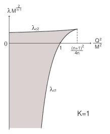
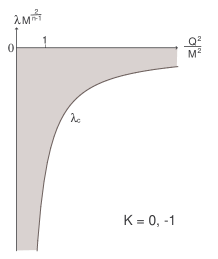
Figure 1: The parameter ranges in which the spacetime contains a regular black hole (the shaded regions).

In general, this solution have a naked singularity or does not have a horizon. As shown in Ref.Kodama.H&Ishibashi2004 , it gives a regular black hole spacetime only when the parameters $M,Q$ and $\lambda$ are in the special regions depicted in Fig.1. In this case, the Einstein space ${\cal K}^{n}$ describes a spatial section of the black hole horizon and at the same time the spatial infinity.

III.2 Uniqueness of black holes

In the static case with $\Lambda=0$, the uniqueness of asymptotically flat regular black holes is now established in higher dimensions as well: all regular solutions are exhausted by the Tangherlini-Schwarzschild solution for the vacuum systemHwang.S1998 ; Gibbons.G&Ida&Shiromizu2003 and by the higher-dimensional Reissner-Norsdtröm solution given by (17) and (19) with $K=1$ and $\Lambda=0$ in the non-degenerate caseGibbons.G&Ida&Shiromizu2002a and the higher-dimensional Majumdar-Papapetrou solutions in the degenerate case for the Einstein-Maxwell systemRogatko.M2003 . Further, it is also proved that the Gibbons-Maeda solution and the Tangherlini-Schwarzschild solution are the only asymptotically flat regular black hole solutions for the Einstein-Maxwell-Dilaton system and for the Einstein-Harmonic-Scalar system, respectivelyGibbons.G&Ida&Shiromizu2002b ; Rogatko.M2002 . However, for $\Lambda\not=0$, nothing is known about the uniqueness, although it was pointed out in Ref. Anderson.M&Chrusciel&Delay2002 that the approach developed by Anderson may also apply to higher-dimensional cases with $\Lambda<0$.

In the rotating case, the higher-dimensional counter-part of the Kerr solution is also known. It is given by the Myers-Perry solutionMyers.R&Perry1986 , which has a spherical horizon and is asymptotically flat. In contrast to the static case, however, this is not the unique asymptotically flat rotating regular solutions in higher dimensions, although the uniqueness holds for supersymmetric black holes in the 5-dimensional $N=1$ minimal supergravity modelReall.H2003 . This is because the horizon topology need not be given by the sphere in higher-dimensions as discussed in Ref. Cai.M&Galloway2001 . In fact, Emparan and ReallEmparan.R&Reall2002a found an asymptotically flat and rotating regular black hole solution in five dimensions whose black hole surface is homeomorphic to $S^{2}\times S^{1}$. Thus, at present, we have two different families of asymptotically flat rotating regular solutions with different horizon topologies. Since more complicated horizon topology is allowed in dimensions greater than 5, it is highly probable that other families of regular solutions exist. However, near the static and spherically symmetric limit, it is likely that a uniqueness theorem holds, as we will see later.

III.3 Stability of black holes

Recently, the author and Ishibashi have shown that for a static charge black hole in higher dimensions represented by (17) and (19), perturbation equations can be also reduced to decoupled 2nd-order master equations of the Schrödinger type, as in four dimensionsKodama.H&Ishibashi2003 ; Kodama.H&Ishibashi2004 . These master equations in higher dimensions, however, have some new features. First, the effective potential $V$ is not positive definite in general. Hence, there may exist an unstable mode. Second, there exists no simple relation between vector and scalar perturbations like the scalar-vector correspondence in four dimensions, for $d=n+2>4$. This implies that stabilities for scalar and vector perturbations should be studied separately. Third, there exist tensor perturbations for $d=n+2>4$.

Now, let us see how these new features affect the stability of static black holes in higher dimensions.

III.3.1 Tensor perturbations

When ${\cal K}^{n}$ is a generic Einstein space, the ${\cal K}^{n}$-coordinates appear in perturbation equations only through the Lichnerowicz operator

$$\hat{\triangle}_{L}h_{ij}=-\hat{D}\cdot\hat{D}h_{ij}-2\hat{R}_{ikjl}h^{kl}+2(n-1)Kh_{ij}.$$ (22)

Hence, by expanding tensor perturbations in terms of the eigentensors of $\hat{\triangle}_{L}$,

$$\hat{\triangle}_{L}{\mathbb{T}}_{ij}=\lambda_{L}{\mathbb{T}}_{ij};\quad{\mathbb{T}}^{i}_{i}=0,\quad\hat{D}^{j}{\mathbb{T}}_{ij}=0,$$ (23)

we obtain a single decoupled equation for $H_{T}^{(2)}$, which can be easily put into the form (8).

In the special case in which ${\cal K}^{n}$ is a constant curvature space, $\hat{\triangle}_{L}$ is expressed as $\hat{\triangle}_{L}=-\hat{D}\cdot\hat{D}+2nK$. Hence, the expansion by ${\mathbb{T}}_{ij}$ is identical to harmonic expansion, and the eigenvalue $\lambda_{T}$ is related to the eigenvalue $k_{T}^{2}$ with respect to $-\hat{D}\cdot\hat{D}$ by $\lambda_{L}=k_{T}^{2}+2nK$. Note that $k_{T}^{2}$ is always non-negative and takes the discrete value $k_{T}^{2}=l(l+n-1)-2\;(l=2,3,\cdots)$ for ${\cal K}^{n}=S^{n}$ ($K=1$).

For neutral black holes, the effective potential for tensor perturbations reads

$$V_{T}=\frac{f}{r^{2}}\left[\lambda_{L}-(3n-2)K+\frac{n(n+2)}{4}f+\frac{n(n+1)M}{r^{n-1}}\right].$$ (24)

When ${\cal K}^{n}$ is maximally symmetric, $V_{T}>0$ outside the horizon since $\lambda_{L}-(3n-2)K=k_{T}^{2}-(n-2)K\geq 0$. Hence, the black hole is stable for a tensor perturbation. In contrast, when ${\cal K}^{n}$ is a generic Einstein space, no general lower bound for $\lambda_{L}$ is known, and generalised static black holes can be unstable against a tensor perturbationGibbons.G&Hartnoll2002 .

Next for charged black holes, since EM field perturbations are not coupled to tensor perturbations of the metric, the master equation is again given by a single equation. The effective potential is given by

$$V_{T}= \frac{f}{r^{2}}\Big{[}\lambda_{L}-(3n-2)K+\frac{n(n+2)f}{4}+\frac{n(n+1)M}{r^{n-1}}$$ (25)

$$\qquad\quad-\frac{n^{2}Q^{2}}{r^{2n-2}}\Big{]}.$$

We can show that this potential is positive definite outside the horizon if $\lambda_{L}-2(n-1)K=k_{T}^{2}+2K\geq 0$. Hence, when ${\cal K}^{n}$ is maximally symmetric, the black hole is stable against tensor perturbations for $K\geq 0$. However, for $K=-1$ ($\lambda<0$), the potential becomes negative near the horizon if $\lambda$ is close to the lower limit $\lambda_{c-}$ in Fig.1. Hence, the black hole might be unstable in this case even when ${\cal K}^{n}$ is maximally symmetric.

III.3.2 S-deformation

For scalar and vector perturbations, we can expand perturbation variables by scalar harmonics ${\mathbb{S}}$ and vector harmonics ${\mathbb{V}}_{i}$ on ${\cal K}^{n}$ satisfying $\hat{\triangle}{\mathbb{S}}=-k^{2}{\mathbb{S}}$ and $\hat{D}\cdot\hat{D}{\mathbb{V}}_{i}=-k_{V}^{2}{\mathbb{V}}_{i}$. For each harmonic, there appear two modes of perturbations, an electromagnetic mode $\Phi_{+}$ and a gravitational mode $\Phi_{-}$. They obey two decoupled equations of the form (11), as in the case of 4D Reissner-Nordström black hole. However, $V_{\pm}$ is not positive definite when $n$ is large, even for spherically symmetric black hole. In order to study the stability for such a system, we utilised the following method that we call the $S$-deformation method.

Let $I$ be the range of $r_{*}$ corresponding to the regular region outside of the horizon, $-\infty<r_{*}<r_{*\infty}$. Here, $r_{*\infty}$ is $+\infty$ for $\lambda\geq 0$, but is finite for $\lambda<0$. Then, in the space $C_{0}^{\infty}(I)$ of smooth functions with compact support, the operator

$$A:=-\frac{d^{2}}{dr_{*}^{2}}+V(r)$$ (26)

is symmetric. We assume that $A$ is extended to a self-adjoint operator in $L^{2}(I)$ by the Friedrichs extension. Then, the lower bound for the spectrum of $A$ coincides with the lower bound of $\omega^{2}=(\Phi,A\Phi)/(\Phi,\Phi)$ ($\Phi\in C^{\infty}_{0}(I)$). Here, for any regular function $S(r)$ on $I$, we have

$$(\Phi,A\Phi)=\int_{I}dr_{*}\left[\left|\left(\frac{d}{dr_{*}}+S(r)\right)\Phi\right|^{2}+\tilde{V}|\Phi|^{2}\right],$$ (27)

where

$$\tilde{V}=V+f\frac{dS}{dr}-S^{2}.$$ (28)

Hence, if we can show that $\tilde{V}$ is non-negative for an appropriate $S$, we can conclude that $\omega^{2}\geq 0$, i.e., the stability of the system.

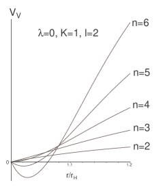
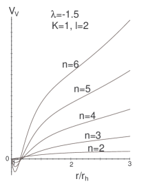
Figure 2: Examples of $V_{V}=V_{V-}$ for $Q=0$.

III.3.3 Vector perturbations

The effective potentials for vector perturbations are given by

$$V_{V\pm}= \frac{f}{r^{2}}\Big{[}k_{V}^{2}+\frac{(n^{2}-2n+4)K}{4}-\frac{n(n-2)}{4}\lambda r^{2}$$ (29)

$$+\frac{n(5n-2)Q^{2}}{4r^{2n-2}}+\frac{-(n^{2}+2)M\pm 2\Delta}{2r^{n-1}}\Big{]},$$

where

$$\Delta^{2}=(n^{2}-1)^{2}M^{2}+2n(n-1)[k_{V}^{2}-(n-1)K]Q^{2}.$$ (30)

These potentials are not positive definite when $n$ is large as illustrated in Fig.2.

Nevertheless, we can show that there exists no unstable mode for most cases, by using the $S$-deformation method. In fact, for $S=nf/2r$, the $S$-deformation yields

$$\tilde{V}_{V\pm}=\frac{f}{r^{2}}\left[m_{V}+\frac{(n^{2}-1)M\pm\Delta}{r^{n-1}}\right],$$ (31)

where $m_{V}=k_{V}^{2}-(n-1)K$. Since $m_{V}\geq 0$, $\tilde{V}_{+}$ is positive definite. Hence, the EM mode of a vector perturbation is always stable. Further, for $K\geq 0$, we can also show that $\tilde{V}_{-}$ is positive definite. Hence, we can conclude that black holes with $K\geq 0$ are stable against vector perturbations. In contrast, for $K=-1$ ($\lambda<0$), $\tilde{V}_{-}$ becomes negative near the horizon when $\lambda$ is close to the critical value $\lambda_{c-}$. In this case, we cannot prove the stability by this method.

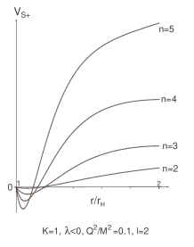
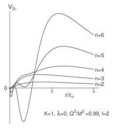
Figure 3: Examples of $V_{S\pm}$

III.3.4 Scalar perturbations

The explicit expressions of the effective potentials $V_{S\pm}$ for scalar perturbations are quite long. So, we only give the graphs of them for some special parameter values in Fig. 3. As these figures show, either of $V_{S+}$ and $V_{S-}$ is not positive definite in general.

However, by the $S$-deformation method again, we can show that the black hole is always stable for the EM mode perturbationKodama.H&Ishibashi2004 . We can also show that asymptotically flat neutral black holes in arbitrary dimensionsIshibashi.A&Kodama2003 and asymptotically dS and AdS neutral black holes in four dimensions are stableKodama.H&Ishibashi2003 . However, the stability of charged black holes has been proved only for special cases. The present status of the perturbative analysis of generalised static black holes is summarised in Table 1.

		Tensor		Vector		Scalar
		$Q=0$	$Q\not=0$	$Q=0$	$Q\not=0$	$Q=0$	$Q\not=0$
$K=1$	$\lambda=0$	OK	OK	OK	OK	OK	$\begin{array}[]{l}d=4,5\ \text{OK}\\ d\geq 6\ \text{?}\end{array}$
	$\lambda>0$	OK	OK	OK	OK	$\begin{array}[]{l}d\leq 6\ \text{OK}\\ d\geq 7\ \text{?}\end{array}$	$\begin{array}[]{l}d=4,5\ \text{OK}\\ d\geq 6\ \text{?}\end{array}$
	$\lambda<0$	OK	OK	OK	OK	$\begin{array}[]{l}d=4\ \text{OK}\\ d\geq 5\ \text{?}\end{array}$	$\begin{array}[]{l}d=4\ \text{OK}\\ d\geq 5\ \text{?}\end{array}$
$K=0$	$\lambda<0$	OK	OK	OK	OK	$\begin{array}[]{l}d=4\ \text{OK}\\ d\geq 5\ \text{?}\end{array}$	$\begin{array}[]{l}d=4\ \text{OK}\\ d\geq 5\ \text{?}\end{array}$
$K=-1$	$\lambda<0$	OK	?	OK	?	$\begin{array}[]{l}d=4\ \text{OK}\\ d\geq 5\ \text{?}\end{array}$	$\begin{array}[]{l}d=4\ \text{OK}\\ d\geq 5\ \text{?}\end{array}$

Table 1: Stability of generalised static black holes

III.4 Perturbative uniqueness

As explained in §II.2.6, we can study the perturbative uniqueness of black holes near the static limit by looking for bounded stationary solutions to the perturbation equations. Actually, we can establish a kind of perturbative uniqueness theorem by this approach. For the limitation of space, we only give an outline of the argument here. The detail will be given in another paperKodama.H2004 .

First of all, note that there exist such solutions with $l=1$ for the vector perturbation equation in the spherically symmetric case ($K=1$) as shown in Ref.Ishibashi.A&Kodama2003 . To be precise, vector harmonics on $S^{n}$ are in one-to-one correspondence to Killing vectors of $S^{n}$, and for each harmonic there exists one stationary solution to the vector perturbation equation. A Killing vector on $S^{n}$ is further in one-to-one correspondence to an antisymmetric matrix of rank $n+1$, and the conjugate class of this matrix is classified by its $N$ eigenvalues, where $N=[(n+1)/2]$ is the rank of ${\rm SO}(n+1)$. Hence, these stationary solutions exactly correspond to the angular momentum freedom of the Myers-Perry solutionMyers.R&Perry1986 .

In the asymptotically flat case, we can show that there exists no other stationary solution for which $\delta g_{\mu\nu}$ are bounded everywhereKodama.H&Ishibashi2003 . Hence, the Myers-Perry solution is the unique regular solution near the static limit. In the asymptotically de Sitter case, we can obtain the same result for the tensor and vector perturbations by using the S-deformation technique. The perturbative uniqueness for the scalar perturbation can also be proved in arbitrary dimensions by applying a similar argument to a master equation that holds only for stationary perturbations. In contrast, the asymptotically anti-de Sitter case is more subtle. In this case, there exist infinitely many solutions with bounded $\delta g_{\mu\nu}$ in addition to the $l=1$ vector perturbations, in accordance with the general result in the four dimensional caseAnderson.M&Chrusciel&Delay2002 . However, if we require the stronger but natural asymptotic condition that every component of the metric perturbation with respect to an background orthonormal basis vanishes at $r\sim\infty$, these extra solutions are excluded.

IV Concluding Remarks

In this article, we have overviewed the present status of the uniqueness and stability issue of black holes in four and higher dimensions. We have seen that the uniqueness and stability are well established for asymptotically flat neutral and static black holes in arbitrary dimensions and for asymptotically flat stationary black holes in four dimensions, but the situation concerning the other cases is quite unsatisfactory. In particular, the classification and stability analysis of rotating black holes and asymptotically de Sitter or anti-de Sitter black holes in higher dimensions are important open problems, although the perturbative analysis can give some useful information as we have shown. In order to solve these problems in the nonperturbative framework, it will be necessary to find a higher-dimensional extension of the rigidity theorem.

References

- (1) Randall, L. and Sundrum, R.: Nucl. Phys. B 557, 79 (1999).
- (2) Antoniadis, I., Arkani-Hamed, N., Dimopoulos, S. and Dvali, G.: Phys. Lett. B 436, 257 (1998).
- (3) Chruściel, P.T.: Helv. Phys. Acta 69, 529 (1996).
- (4) Heusler, M.: Black Hole Uniqueness Theorem (Cambridge Univ. Press, 1996); Living Reviews 1, 6 (1998).
- (5) Hawking, S. and Ellis, G.: The large scale structure of space-time (Cambridge Univ. Press, 1973).
- (6) Chruściel, P.T. and Wald, R.M.: Class. Quant. Grav. 11, L147 (1994).
- (7) Rácz, I. and Wald, R.M.: Class. Quant. Grav. 13, 539 (1996).
- (8) Chruściel, P.T.: Class. Quant. Grav. 16, 689 (1999); ibid, 661 (1999).
- (9) Weinstein, G.: Trans. Amer. Math. Soc. 343, 899 (1994).
- (10) Weinstein, G.: Comm. Partial Differential Equations 21, 1389 (1996).
- (11) Gibbons, G.W. and Maeda, K.: Nucl. Phys. B 298, 741 (1988).
- (12) Masood-ul-Alam, A.: Class. Quant. Grav. 10, 2649 (1993).
- (13) Mars, M. and Simon, W.: Adv. Theor. Math. Phys. 6, 279 (2003).
- (14) Gibbons, G.W., Ida, D. and Shiromizu, T.: Phys. Rev. D 66, 044010 (2002).
- (15) Rogatko, M.: Phys. Rev. D 59, 104010 (1999).
- (16) Rogatko, M.: Class. Quant. Grav. 19, L151 (2002).
- (17) Heusler, M.: Class. Quant. Grav. 12, 2021 (1995).
- (18) Bartnik, R. and McKinnon, J.: Phys. Rev. Lett. 61, 141 (1988).
- (19) Volkov, M.S. and Galtsov, D.V.: Sov. J. Nucl. Phys. 51, 1171 (1990).
- (20) Künzle, H.P. and Masood-ul-Alam, A.: J. Math. Phys. 31,928 (1990).
- (21) Straumann, N. and Zhou, Z.-H.: Phys. Lett. B 237, 353 (1990).
- (22) Bizon, P.: Phys. Lett. B 259, 53 (1991).
- (23) Zhou, Z.-h. and Straumann, N.: Nucl. Phys. B 360, 180 (1991).
- (24) Droz, S., Heusler, M. and Straumann, N.: Phys. Lett. B 268,371 (1991).
- (25) Heusler, M., Droz, S. and Straumann, N.: Phys. Lett. B 271, 61 (1991); ibid. 285, 21 (1992).
- (26) Heusler, M., Straumann, N. and Zhou, Z.-H.: Helv. Phys. Acta 66, 614 (1993).
- (27) Anderson, M. T.: math.DG/0105243 (2001).
- (28) Anderson, M. T.: math.DG/0104171 (2001).
- (29) Anderson, M.T., Chrusciël, P.T. and Delay, E.: JHEP 0210, 063 (2002).
- (30) Wald, R. M.: gr-qc/9710068 (1997).
- (31) Vishveshwara, C.: Phys. Rev. D 1, 2870 (1970).
- (32) Price, R.: Phys. Rev. D 5, 2419 (1972).
- (33) Wald, R.M.: J. Math. Phys. 20, 1056 (1979).
- (34) Wald, R.M.: J. Math. Phys. 21, 218 (1980).
- (35) Chandrasekhar, S.: The Mathematical Theory of Black Holes (Clarendon Press, 1983).
- (36) Kodama, H. and Ishibashi, A.: Prog. Theor. Phys. 111, 29 (2004).
- (37) Whiting, B.: J. Math. Phys. 30, 1301 (1989).
- (38) Bardeen, J.: Phys. Rev. D 22, 1882 (1980).
- (39) Kodama, H. and Sasaki, M.: Prog. Theor. Phys. Suppl. 78, 1 (1984).
- (40) Kodama, H., Ishibashi, A. and Seto, O.: Phys. Rev. D 62, 064022 (2000).
- (41) Gibbons, G.W. and Hartnoll, S.A.: Phys. Rev. D 66, 064024 (2002).
- (42) Regge, T. and Wheeler, J.: Phys. Rev. 108, 1063 (1957).
- (43) Zerilli, F.: Phys. Rev. Lett. 24, 737 (1970).
- (44) Kodama, H. and Ishibashi, A.: Prog. Theor. Phys. 110, 701 (2003).
- (45) Moncrief, V.: Phys. Rev. D 9, 2707 (1974).
- (46) Zerilli, F.: Phys. Rev. D 9, 860 (1974).
- (47) Poisson, E. and Israel, W.: Phys. Rev. D 41, 1796 (1990).
- (48) Cardoso, V. and Lemos, J.P.S.: Phys. Rev. D 64, 084017 (2001).
- (49) Chandrasekhar, S. and Detweiler, S.: Proc. R. Soc. London A 344,441 (1975).
- (50) Carter, B.: Phys. Lett. A 26, 399 (1968).
- (51) Tangherlini, F.R.: Nuovo Cimento 27, 636 (1963).
- (52) Birmingham, D.: Class. Quantum Grav. 16, 1197 (1999).
- (53) Hwang, S.: Geometriae Dedicata 71, 5 (1998).
- (54) Gibbons, G.W., Ida, D. and Shiromizu, T.: Prog. Theor. Phys. Suppl. 148, 284 (2003).
- (55) Gibbons, G.W., Ida, D. and Shiromizu, T.: Phys. Rev. Lett. 89, 041101 (2002).
- (56) Rogatko, M.: Phys. Rev. D 67, 084025 (2003).
- (57) Myers, R. and Perry, M.: Ann. Phys. 172, 304 (1986).
- (58) Reall, H.: Phys. Rev. D 68, 024024 (2003).
- (59) Cai, M. and Galloway, G.: Class. Quant. Grav. 18, 2707 (2001).
- (60) Emparan, R. and Reall, H.S.: Phys. Rev. Lett. 88, 101101 (2001).
- (61) Ishibashi, A. and Kodama, H.: Prog. Theor. Phys. 110, 901 (2003).
- (62) Kodama, H.: hep-th/0403239 (2004).