Order parameters with higher dimensionful composite fields

Abstract

We discuss the possibility of the spontaneous symmetry breaking characterized by order parameters with higher dimensionful composite fields. By analyzing general Ginzburg-Landau potential for a complex scalar field $\phi=\phi_{1}+\mathrm{i}\phi_{2}$ with $O(2)$ symmetry, we demonstrate that a phase characterized by $\langle\phi_{1}^{2}-\phi_{2}^{2}\rangle\neq 0$ with $\langle\phi_{1}\rangle=\langle\phi_{2}\rangle=0$ is realized in a certain parameter region. To clarify the driving force to favor this phase, we study the $O(2)$ $\phi^{6}$ theory in three dimensions.

The spontaneous symmetry breaking (SSB) should be enumerated as one of the key concepts in modern physics, in particular in condensed matter and elementary particle physics nam61 . Even if some global symmetry is manifest in the Hamiltonian, the ground state and excited spectra do not have to reflect the symmetry manifestly. The order parameter, which is a measure of SSB, is defined by the ground state expectation value of an operator being variant under the symmetry transformation. The choice of the operator is constrained by the symmetry breaking pattern. The purpose of this Letter is to draw attention to the issue of SSB through such order parameters with higher canonical dimensions. As we will argue, unbroken discrete groups generally require operators with higher canonical dimensions.

Let us first give a summary to construct generic order parameters. Suppose $X$ and $Q_{a}$ be a symmetry group and the generators of the symmetry transformation, respectively. We take an operator $\mathcal{O}$ which transforms non-trivially under $Q_{a}$; $[\mathrm{i}Q_{a},\mathcal{O}]\neq 0$. SSB takes place if we have such an $\mathcal{O}$ that $\langle 0|[\mathrm{i}Q_{b},\mathcal{O}]|0\rangle\neq 0$ for some $b$ . If $Q_{b}$ is a generator of $X$ but is outside of its subgroup $Y$, the symmetry is spontaneously broken from $X$ to $Y$ with an order parameter $\langle 0|[\mathrm{i}Q_{b},\mathcal{O}]|0\rangle$. $\mathcal{O}$ can be chosen to be any operators as long as it is invariant under $Y$.

In particular, if $Y$ contains a discrete subgroup of $X$, SSB generally requires higher dimensionful composite operators for $\mathcal{O}$ because the elementary operators are not invariant in $Y$. We pursue such exotic realization of SSB not only for academic interest but for phenomenological importance. In Quantum Chromodynamics (QCD) we sometimes encounter possibilities of higher dimensionful operators. A well-known example is the four-quark operator introduced for a non-standard chiral symmetry breaking pattern in $N_{\text{f}}$-flavors ste98 where $X=SU_{\text{L}}(N_{\text{f}})\times SU_{\text{R}}(N_{\text{f}})$ with $Y=SU_{\text{V}}(N_{\text{f}})\times Z_{\text{A}}(N_{\text{f}})$. Although this is proven to be forbidden in QCD at zero and finite temperature, it may be realized at finite baryon chemical potential. Interestingly enough, the remaining $Z_{\text{A}}(N_{\text{f}})$ symmetry could change the hadron spectrum significantly gir01 . Exotic hadron spectrum in a similar natureson00 is indeed known to be realized in the color-flavor-locking (CFL) phase in color superconductivity where $U_{\text{B}}(1)$ is broken down to $Z(2)$ subgroup alf99 . In particular, the existence of light kaonic excitations associated with this SSB opens a possibility for the kaon condensation in the CFL phase bed02 . Therefore, in connection with these phenomenological concerns, it is an important issue to probe SSB with an unbroken discrete subgroup and with higher dimensionful order parameter from the generic point of view.

In order to look into the problem in a concrete setting, let us take an $O(2)$ symmetric model with one complex scalar field $\phi=\phi_{1}+\mathrm{i}\phi_{2}$. If we take $\mathcal{O}=\mathrm{Im}\phi=\phi_{2}$ which is not symmetric in any of the $O(2)$ transformation, we have $\delta\phi_{2}\propto\mathrm{Re}\phi=\phi_{1}$. It follows that the order parameter for the symmetry breaking pattern $X=O(2)\to\text{none}$ is $\langle\phi_{1}\rangle\equiv\langle 0|\phi_{1}|0\rangle$. This is, however, not a unique symmetry breaking pattern possible. Consider $X=O(2)$ and $Y=Z_{2}$ with $Z_{2}$ being a discrete subgroup with the operation; $\phi_{1,2}\to-\phi_{1,2}$. In this case $\mathcal{O}=\mathrm{Im}\phi^{2}=2\phi_{1}\phi_{2}$, which is $Y$ invariant, leads to an order parameter,

$$\mathrm{Re}\langle\phi^{2}\rangle=\langle\phi_{1}^{2}-\phi_{2}^{2}\rangle.$$ (1)

Note that the difference between $\langle\phi_{1}^{2}\rangle$ and $\langle\phi_{2}^{2}\rangle$ is an appropriate order parameter instead of the individuals because the common constant cancels out in the former. One can construct $k$-th composite order parameters for $O(2)\to Z_{k}$ in the same way;

$$\mathrm{Re}\langle\phi^{k}\rangle.$$ (2)

If $\mathrm{Re}\langle\phi\rangle$ has a non-vanishing value, the $O(2)$ symmetry is totally broken so that the higher dimensionful order parameters, $\mathrm{Re}\langle\phi^{k}\rangle$, are non-zero for all $k\geq 1$. The SSB with $O(2)\to Z_{k}$ can be characterized by the condition; $\mathrm{Re}\langle\phi\rangle=\cdots=\mathrm{Re}\langle\phi^{k-1}\rangle=0$ and yet $\mathrm{Re}\langle\phi^{k}\rangle\neq 0$.

Application of the above argument to $O(N)$ symmetric models with $N>2$ is straightforward. For the SSB pattern, $O(N)\to O(2)\to Z_{k}$, the higher dimensionful order parameter can be defined in the same way as above with respect to the $O(2)$ subgroup.

Now we shall go on to investigate whether there is a situation where the above SSB pattern, $O(2)\to Z_{k}$, is indeed realized. We will focus on a simplest case, $k=2$, namely the phase characterized by $\langle\phi_{1}^{2}-\phi_{2}^{2}\rangle$. For later purpose, we introduce complex variables $W$ and $H$, and a real variable $F$ as follows,

$$\begin{split}&W=\langle\phi^{2}\rangle=\langle\phi_{1}^{2}-\phi_{2}^{2}\rangle+2\mathrm{i}\langle\phi_{1}\phi_{2}\rangle,\\ &F=\langle\phi^{\dagger}\phi\rangle=\langle\phi_{1}^{2}+\phi_{2}^{2}\rangle,\\ &H=\langle\phi\rangle=\langle\phi_{1}+\mathrm{i}\phi_{2}\rangle.\end{split}$$ (3)

To clarify the phase structure in the $W$-$F$-$H$ space, let us consider a Ginzburg-Landau type effective potential with $O(2)$ symmetry up to terms of $\phi^{6}$ order which are at least necessary to induce a phase with $W\neq 0$;

$$V_{\text{eff}}[W,F,H]$$

$$=(d_{1}+d_{2}F+d_{3}F^{2})|H|^{2}+(d_{4}+d_{5}F)|H|^{4}+d_{6}|H|^{6}$$

$$\qquad+(c_{1}+c_{2}F)(W^{\dagger}H^{2}+H^{\dagger 2}W)$$

$$\qquad+a_{1}F+a_{2}F^{2}+a_{3}F^{3}+(b_{1}+b_{2}F)|W|^{2}.$$ (4)

The coefficients $a_{i}$, $b_{i}$, $c_{i}$, and $d_{i}$ are considered to be arbitrary coupling constants at the present stage. Taking a specific model with $O(2)$ symmetry, one may determine their magnitudes and relations. For more than two dimensions, one needs to subtract the short distant singularities in $F$ and $W$ to make them finite. This will be discussed in more detail later and we assume a simple cutoff in the short distant part here.

The standard phase corresponding to the SSB pattern, $O(2)\to\text{none}$, is characterized by $H\neq 0$ (and thus $W\neq 0$), while the non-trivial phase corresponds to $W\neq 0$ with $H=0$. Note that $F\neq 0$ in both cases. For convenience, we call the latter phase as “the WFH phase” after the notation in Eq. (3). To find the condition for the WFH phase, we choose $d_{i}$ appropriately so as to realize $H=0$. Then the GL potential is reduced to only the terms containing $a_{i}$ and $b_{i}$ in Eq. (4). Among these coupling constants, we can eliminate two of them by rescaling $F$ (and $W$) and coupling constants. Then one finds

$$V_{\text{eff}}[W,F]=a_{1}^{\prime}F\pm F^{2}+F^{3}+(b_{1}^{\prime}+b_{2}^{\prime}F)W^{2},$$ (5)

where $W$ is chosen to be real and positive without loss of generality and as a consequence we have a constraint, $F\geq W\geq 0$. Note that the sign of the $F^{3}$ term should be positive to guarantee the stability of the potential, while it is not necessary for the coefficient of the $F^{2}$ term.

An instability toward $W\neq 0$ is induced by the negative $W^{2}$ term in Eq. (5). Therefore, once the instability to the WFH phase occurs, $W=F$ is realized because of the constraint $F\geq W\geq 0$. To see the competition between the symmetric phase ($W=0$) and the WFH phase ($W=F\neq 0$), we compare the potential energies at two possible global minima as

$$V_{\text{eff}}[W=0,F] =aF\pm F^{2}+F^{3},$$ (6)

$$V_{\text{eff}}[W=F,F] =aF+bF^{2}+cF^{3},$$ (7)

where $a=a_{1}^{\prime}$, $b=\pm 1+b_{1}^{\prime}$, and $c=1+b_{2}^{\prime}$.

The gap equation for $F$ is obtained from $\partial V_{\text{eff}}/\partial F=0$. Eq. (6) has a global minimum at $F_{0}>0$, i.e., $V_{\text{eff}}[F_{0},0]<V_{\text{eff}}[0,0]=0$ is satisfied for $a<0$ (for $+F^{2}$) and for $a<1/4$ (for $-F^{2}$). On the other hand, Eq. (7) has a global minimum at $F_{1}>0$ either for ($a>0$, $b<0$, $b^{2}>4ac$) or for $a<0$. Then the condition $V_{\text{eff}}[F_{1},F_{1}]<V_{\text{eff}}[0,F_{0}]$ yields an inequality;

$$\begin{split}&\biggl{\{}-(1-3a)^{3/2}+\frac{(b^{2}-3ac)^{3/2}}{c^{2}}\biggr{\}}\\ &\quad+\biggl{(}\pm 1-\frac{b^{3}}{c^{2}}\biggr{)}-\frac{9}{2}\biggl{(}\pm a-\frac{ab}{c}\biggr{)}>0.\end{split}$$ (8)

Shown in Fig. 1 is the above condition for the negative $F^{2}$ term in Eqs. (5) and (6). The region below the surface corresponds to the parameters where the WFH phase can exist. When the $F^{2}$ term is positive, it is sufficient to consider the potential only up to the $F^{2}$ term in order to guarantee the stability of the potential, and the WFH phase is realized for $a<0$ and $0<b<1$. The message here is that there is always a wide parameter region in the Ginzburg-Landau type effective potential so that the WFH phase is realized.

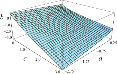
Figure 1: In the region below the surface, the WFH phase is favored.

To study microscopic mechanism to induce the instability toward $W\neq 0$ in field theoretical models, let us consider an $O(2)$ $\phi^{6}$ model in three spatial dimensions with the Hamiltonian density,

$$\mathcal{H}=\frac{1}{2}|\nabla\phi|^{2}+\frac{g_{2}}{2}|\phi|^{2}+\frac{g_{4}}{4}|\phi|^{4}+\frac{g_{6}}{6}|\phi|^{6}.$$ (9)

We assume $g_{6}>0$ for stability of the system. If the symmetry group is $O(4)$ instead of $O(2)$, the model is considered as the 3d effective theory to describe the tricritical behavior of the chiral phase transition in QCD at finite temperature and baryon density step98 .

We treat the model in the Cornwall-Jackiw-Tomboulis (CJT) formalism cor74 which is best suited for studying the system with composite order parameters. The effective action is given in general by

$$\Gamma[G,H]=I_{0}[H]+\frac{1}{2}\mathrm{Tr}\ln G^{-1}+\frac{1}{2}\mathrm{Tr}\,G_{0}^{-1}[H]\,G+\Gamma_{2}[G,H],$$ (10)

where $I_{0}[H]$ and $G_{0}[H]$ are the tree-level potential and propagator, respectively. $G$ is the full propagator satisfying $\delta\Gamma/\delta G=0$. $\Gamma_{2}$ represents the contributions from 2 particle irreducible (2PI) diagrams with $G$.

Taking into account the terms up to leading order 2PI diagrams, which is equivalent to the Hartree-Fock (HF) approximation in many-body theories, $G$ can be written by the dynamical mass $m_{a}$ of the field $\phi_{a}$. Then the expectation value of the local composite operator $G_{ab}(x,x)=\langle\phi_{a}\phi_{b}\rangle$ reads

$$S_{ab} \equiv G_{ab}(x,x)=\delta_{ab}\int^{\Lambda}\frac{\mathrm{d}^{3}p}{(2\pi)^{3}}\frac{1}{p^{2}+m_{a}^{2}}$$

$$=\delta_{ab}\frac{1}{2\pi^{2}}\biggl{\{}\Lambda-|m_{a}|\arctan\Bigl{(}\frac{\Lambda}{|m_{a}|}\Bigr{)}\biggr{\}},$$ (11)

where $\Lambda$ is the three dimensional cutoff of the loop integral. The term proportional to $\Lambda$ in Eq. (11) corresponds to the short distance part independent of $m_{a}$. Thus, the WFH phase, in which $\langle\phi_{1}^{2}-\phi_{2}^{2}\rangle=S_{11}-S_{22}\neq 0$ is realized, can be characterized by $m_{1}\neq m_{2}$ within the present approximation.

From now on we take $H=0$ by hand as before to focus on the phase with $W\neq 0$. The dynamical masses, $m_{a}$, are determined by the gap equation derived from the variation of the CJT potential or from the self-consistent HF equation;

$$\frac{m_{a}^{2}}{2}=\frac{g_{2}}{2}+\frac{g_{4}}{4}\Bigl{(}\sum_{b}S_{b}+2S_{a}\Bigr{)}$$

$$\;+\frac{g_{6}}{6}\biggl{\{}\Bigl{(}\sum_{b}S_{b}\Bigr{)}^{2}+4S_{a}\sum_{b}S_{b}+2\sum_{b}S_{b}^{2}+8S_{a}^{2}\biggr{\}},$$ (12)

where $S_{a}\equiv S_{aa}$ (see Eq. (11)). Each term in Eq. (12) has the graphical representation as shown in Fig. 2.

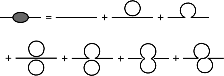
Figure 2: An illustration of the gap equation, Eq. (12). The Hartree terms correspond to those with fully disconnected loops (the second term in the first row and the first term in the second row). Other terms with loop(s) are the Fock terms.

The genuine Hartree terms in the right hand side of Eq. (12) or the fully disconnected graphs in Fig. 2 are index-blind and give equivalent contributions to $m_{1}$ and $m_{2}$. Hence, if we take only Hartree terms, the standard solution, $m_{1}=m_{2}$, is obtained. On the other hand, the Fock terms in the right hand side of Eq. (12) are connected to the external lines and depend on the external index $a$. This leads to a possibility for $m_{1}\neq m_{2}$.

Of course, the above argument does not guarantee the realization of an asymmetric solution, because $m_{1}=m_{2}$ is also a solution even if we have Fock terms. To study which solution is more stable, we have calculated the CJT effective potential written in terms of $f=|m_{1}|+|m_{2}|$ and $w=|m_{1}|-|m_{2}|$. For small $m_{a}$, they are related to $F=S_{11}+S_{22}$ and $W=S_{11}-S_{22}$ as

$$\begin{split}&F=\frac{1}{2\pi^{2}}\Bigl{(}2\Lambda-\frac{\pi}{2}f+O(|m_{a}|^{2})\Bigr{)},\\ &W=-\frac{1}{2\pi^{2}}\Bigl{(}\frac{\pi}{2}w+O(|m_{a}|^{2})\Bigr{)}.\end{split}$$ (13)

For convenience, we use $w$ and $f$ as basic variables in the following.

Assuming that $m_{a}$ are small enough compared to $\Lambda$, we expand the CJT potential in terms of $f$ and $w$ up to the same order with Eq. (5);

$$\bar{V}_{\text{eff}}[w,f] =-\frac{\bar{g}_{2}}{2}f+\frac{\bar{g}_{4}}{2}f^{2}+(1-\bar{g}_{6})f^{3}$$

$$\qquad+\frac{1}{2}\Bigl{\{}\frac{\bar{g}_{4}}{2}+3(2-\bar{g}_{6})f\Bigr{\}}w^{2}.$$ (14)

Note that $w^{2}$ terms come from the Fock contributions and the bare coupling constants and the potential are redefined as

$$\begin{split}\bar{g}_{6}&=\frac{3}{2\pi^{2}}g_{6},\qquad\bar{g}_{4}=\frac{24}{\pi}g_{4}+\frac{36}{\pi^{3}}g_{6},\\ \bar{g}_{2}&=24g_{2}-\frac{48}{\pi^{2}}g_{4}-\frac{144}{\pi^{4}}g_{6},\\ \bar{V}_{\text{eff}}&=96\pi V_{\text{eff}}\end{split}$$ (15)

with the cutoff $\Lambda$ being set to 1. The stability of the system at large $f$ leads to a condition, $\bar{g}_{6}<1$ (or equivalently $g_{6}<2\pi^{2}/3$ bar84 ). Although the definition of the order parameter is slightly different from the general analysis in Eq. (5), obtained effective potential has the same structure. The correspondence becomes even transparent if we rescale $\bar{V}_{\text{eff}}$ and $f$ (and $w$) to eliminate two of the coefficients in Eq. (14) to obtain

$$V_{\text{eff}}[w,f]=a_{1}f\pm f^{2}+f^{3}+\Bigl{(}\pm\frac{1}{2}+b_{2}f\Bigr{)}w^{2},$$ (16)

where $b_{2}>3$, which comes from $\bar{g}_{6}<1$. In the following, we choose the negative signs in the $f^{2}$ and $w^{2}$ terms in Eq. (16) because the $-\frac{1}{2}w^{2}$ term, which originates from the Fock contribution, induces the instability toward the WFH phase.

The condition that $V_{\text{eff}}[w=m_{1},f=m_{1}]$ (the WFH phase) has at least a local minimum with respect to $m_{1}$ leads to $a_{1}(b_{2}+1)<3/4$. This is shown by the left hand side of the dotted curve in Fig. 3. The stability in the $m_{2}$ direction requires $3(b_{2}+1)+4a_{1}b_{2}(b_{2}-1)+\sqrt{3}\sqrt{3-4a_{1}(b_{2}+1)}>0$, which is shown by the right hand side of the solid curve in Fig. 3. As we mentioned, $b_{2}>3$ is necessary for the stability of the potential at large $f$. As a result, the WFH phase is allowed at least as a local-minimum in the gray region in Fig. 3. It can be, however, shown that it is not a global minimum but a meta-stable phase. In fact, by comparing Eq. (16) with $f=w$ and Eq. (7), one finds $a=a_{1}$, $b=-3/2$, and $c=1+b_{2}>4$. This parameter set is too restrictive and can not satisfy the condition Eq. (8) which is necessary for the absolute stability.

Even though it is only a meta-stable state, an important message here is that the 3d $O(2)$ $\phi^{6}$ theory in the HF approximation embodies a driving force (the Fock term) leading toward the WFH phase. Whether this new phase is indeed realized as a true ground state or not should be examined in an approach beyond the HF approximation or by numerical simulations. In $O(N>2)$ theories, the Fock term is suppressed relative to the Hartree term for large $N$. Therefore the WFH phase driven by the Fock term is expected in small $N$ instead of in large $N$.

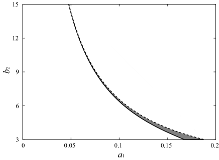
Figure 3: Meta-stable WFH phase is allowed in the gray region.

In summary, we have studied higher dimensionful order parameters associated with the dynamical symmetry breaking which leaves manifest discrete symmetry. By taking a complex scalar field $\phi$ and its Ginzburg-Landau potential as an example, we have given a general criterion to have a novel symmetry breaking pattern $O(2)\to Z_{2}$ characterized by the order parameter $\mathrm{Re}\,\langle\phi^{2}\rangle\neq 0$. We have demonstrated that the Hartree-Fock approximation to the 3d $O(2)$ $\phi^{6}$ theory gives such a novel phase at least as a meta-stable state. Whether the new phase exists as a true ground state beyond the HF approximation is an open question to be studied. We have assumed the stability around $\langle\phi\rangle=0$ in this Letter; further studies of the interplay among the three condensates, $\langle\phi\rangle$, $\langle|\phi|^{2}\rangle$, and $\langle\phi^{2}\rangle$ should be also pursued. The lesson we can learn from our results in this Letter is that SSB through higher dimensionful order parameters is not so peculiar and may possibly be realized in more complex systems. Applications of the idea to e.g. gauge field theories and condensed matter systems are interesting future problems to be studied.

Acknowledgments: Y. W. is grateful to Ayumu Sugita for his crucial suggestions. K. F. is supported by Japan Society for the Promotion of Science for Young Scientists. This work is partially supported by the Grants-in-Aid of the Japanese Ministry of Education, Science and Culture (No. 15540254) and the U.S. Department of Energy (D.O.E.) under cooperative research agreement #DF-FC02-94ER40818.

References

- (1) Y. Nambu and G. Jona-Lasinio, Phys. Rev. 122, 345 (1961). J. Goldstone, Nuovo Cimento 19, 154 (1961). J. Goldstone, A. Salam, and S. Weinberg, Phys. Rev. 127, 965 (1962).
- (2) J. Stern, eprint: hep-ph/9801282. I.I. Kogan, A. Kovner, and M.A. Shifman, Phys. Rev. D 59, 016001 (1999).
- (3) L. Girlanda, J. Stern, and P. Talavera, Phys. Rev. Lett. 86, 5858 (2001).
- (4) D.T. Son and M.A. Stephanov, Phys. Rev. D 61, 074012 (2000).
- (5) M. Alford, K. Rajagopal, and F. Wilczek, Nucl. Phys. B537, 443 (1999). M. Alford, J. Berges, and K. Rajagopal, Nucl. Phys. B558, 219 (1999).
- (6) P.F. Bedaque and T. Schäfer, Nucl. Phys. A697, 802 (2002).
- (7) M.A. Stephanov, K. Rajagopal, and E.V. Shuryak, Phys. Rev. Lett. 81, 4816 (1998); Phys. Rev. D 60, 114028 (1999). K. Fukushima, Phys. Rev. C 67, 025203 (2003). Y. Hatta and T. Ikeda, Phys. Rev. D 67, 014028 (2003).
- (8) J.M. Cornwall, R. Jackiw, and E. Tomboulis, Phys. Rev. D 10, 2428 (1974).
- (9) W.A. Bardeen, M. Moshe, and M. Bander, Phys. Rev. Lett. 52, 1188 (1984).