Dynamics of phase transition in (3+1) dimensional scalar $\phi^{4}$ theory

Abstract

We use the variational approximation with double Gaussian type trial wave-functional approximation, in which we use the square root of the dispersion of the zero-mode wave-function as an order parameter, to study the out of equilibrium quantum dynamics of time-dependent second order phase transitions in (3+1) dimensions. We study the time evolution of symmetric states of scalar $\lambda\phi^{4}$ theory in several situations by properly treating the effect of the $\lambda\phi^{4}$ interaction. We also calculate the effective action and the effective potential of the theory with the precarious renormalization. We show that the presence of a quenching of the mass-squared leads to second order phase transition nontrivially since the vacuum structure changes by absorbing the energy required for quenching, even though there is no symmetry breaking in the effective potential of the theory without quenching process. We also calculate the equal time correlation function, and then evaluate the correlation length as a function of the mass-squared. The time dependence of the correlation length varies depending on how the mass-squared changes in time. For constant mass-squared it gives the classical Cahn-Allen relation, and it leads to different relations for other time-dependence of the mass-squared. We also show that there exists a propagating spatial correlation after termination of the phase transition process in addition to the correlation corresponding to the formation and growth of domains.

I Introduction

In recent years, there has been strong interest in the dynamics of the quantum fields out of equilibrium appearing in the evolution of the early universe or in the process of phase transition guth ; vilenkin . The formation of topological defects, the dynamics of inflation of the universe, and the inflationary reheating have been studied on the basis of scalar field model. The domain formation and growth boyanovsky were studied in the out of equilibrium second order phase transition using the Hartree-Fock approximation. During a second order phase transition, the time scale of relaxation of the scalar field lags behind the time scale of change of the effective potential. Consequently, the field evolves out of equilibrium as it tries to relax to a new vacuum, giving rise to a nonvanishing vacuum expectation value. Such nonequilibrium effects play a crucial role in topological defect formation in condensed matter systems as well as in the early universe gill ; ibaceta ; stephens . Kibble first showed how the correlation length is crucial in determining the initial density of topological defects kibble . These ideas were elaborated by Zurek who proposed that it may be possible to quantitatively test the Kibble mechanism of defect formation in condensed matter systems such as superfluid He⁴ zurek . He argued that, because of the phenomenon of critical slowing down near the phase transition point, the correlation length relevant for determining the initial density of the defects is not the equilibrium correlation length at the Ginzburg temperature but that at the time when the field dynamics essentially freezes out. He also found a power law behavior in the dependence of the correlation length on the quench rate. There have been various attempts to experimentally test the Kibble-Zurek prediction of initial defect density laguna . A comprehensive review on these issues is given in Ref. rivers .

One crucial lesson provided by these studies is the importance of using time-dependent techniques to study processes of the system with explicit time-dependence. It has been repeatedly shown that classical and one-loop effective potentials are poorly defined and of little use in such dynamical systems. Another common theme is the importance of non-linear corrections to the linear dynamics. In these directions, the dynamics of spinodal decomposition in inflationary cosmology using the closed time path formalism of quantum field theory out of equilibrium combined with the non-perturbative Hartree approximation was analyzed in Ref. cormier . A feature common to all such phase transitions is the evolution far away from equilibrium and the exponential growth of the soft (long wavelength) modes, which necessarily lead to domain growth. Finite temperature field theory based on equilibrium or quasi-equilibrium methods does not describe all the processes of nonequilibrium evolution even though the imaginary part of the complex effective action yields the decay rate weinberg . To treat such nonequilibrium quantum evolution properly, Schwinger and Keldysh first introduced the closed-time formalism schwinger . The closed-time formalism and the $1/N$ expansion method have been applied to nonequilibrium $\lambda\phi^{4}$ theory to explain the phenomenon of domain growth cooper . Recently, the Liouville-von Neumann approach has been developed that unifies both the functional Schrödinger equation for quantum evolution and the quantum Liouville equation for quantum statistical mechanics spkim . The renormalization of field theory in quenched second order phase transitions was discussed in Ref. spkim2 in this context.

An obstacle in discussing the phase transition of the scalar field in (3+1) dimensions is that there is no symmetry breaking in the Gaussian effective potential of the theory with the precarious renormalization stevenson , which is the only relevant renormalization scheme which does not require non-trivial assumptions such as the existence of a large momentum cutoff, large $N$ limit of $O(N)$ scalar field, or the autonomous renormalization stevenson2 ; jhyee . On the other hand, there have been various studies on the 2nd order phase transitions of the scalar $\phi^{4}$ theory in (3+1)dimensions in relation to the $O(N)$ symmetric theory cooper , the non-equilibrium field theories spkim2 ; cormier , and the theory with high momentum cutoff consoli . Most of these studies consider the region in which the phase transition begins, where the dynamical behavior of the unstable modes are the main interest. It is an interesting question to which vacuum the system will settle down after the transition since there is no vacuum with non-zero order parameter in the static theory described by the effective potential. In this paper we answer this question by showing that the vacuum structure of the scalar field theory changes when the second order phase transition occurs.

The variational approach for the scalar field theory using the Gaussian effective potential was well studied in Refs. stevenson ; cea ; barns , and references therein. The renormalizability and the initial value problem for the Gaussian approximation of time-dependent scalar systems are checked in  cooper3 ; pi1 . Many authors have studied the symmetry breaking phase structures in the large $N$ approximation baacke . Non-equilibrium dynamics of symmetry breaking cooper2 and the second order phase transition spkim have also been studied in the Gaussian frame work. The Hartree-Fock method has been popular and useful in studying the nonequilibrium evolution of the field cooper . Even though the renormalization is well understood even for nonequilibrium fields in Refs. cooper a systematic and explicit renormalization scheme of the effective action has not been properly addressed for the systems undergoing phase transitions at least in (3+1) dimensions. In this paper, we propose such a renormalization scheme of the effective action for systems describing phase transitions.

As field theory models for the second order phase transition, some exactly solvable models of the free scalar field were studied in Ref. spkim , in which it was proposed that the exponential growth of the spinodal instability may ends at the spinodal line because of the back-reaction of the scalar field. The spinodal instability leads to the domain formation and growth boyanovsky , which is determined by the equal time correlation functions. The formation and growth of the domains were studied up to the point where the phase transition process ends. It is generally believed that the domain becomes static once it is formed without other dynamics involved. In this paper, by studying the spatial correlation functions determined by the approximation method proposed in Ref. kim , we show that there exists another propagating correlations after the transition process is over in addition to the static domain.

Recently, the present authors have developed a new quartic exponential type variational approximation kim1 which is suitable for double well type potentials in the quantum mechanical context. This approach was applied to the zero mode of the scalar field kim , where we have renormalized the equations of motion which describes the symmetry breaking phenomena starting from the symmetric states of the scalar $\lambda\phi^{4}$ theory in three and four dimensions. In the present paper, we use some of these results summarized in Sec. II.

The article is organized as follows. In Sec. II, we briefly present the double Gaussian type wave-functional approximation to the $\lambda\phi^{4}$ theory. Then, we introduce the Klein-Gordon like mode solutions, with which we rewrite the Hamiltonian of the system so that it includes the temperature of the initial equilibrium state. In Sec. III, we calculate the effective action and potential of the interacting scalar field with fixed mass in which the tachyonic mode described by negative mass-squared is included. It is shown that the typical effective potential develops a new local minima at the non-vanishing expectation value of the field at which point the mass vanishes even though the vacuum still presents at the symmetric point of order parameter. Sec. IV is devoted to the analysis of an exact mode solution of the field equation in which the mass-squared varies from positive to negative values. We obtain several asymptotic behaviors of the solution such as the instantaneous quenching, $t\rightarrow\infty$ limit, and ultra-violet (UV) limit. These are used in Sec. V to obtain the WKB approximation for the general field equation. In Sec. V, we study the self-interacting scalar field system with instantaneous quenching at $t=0$. After the quenching we allow the mass-squared freely evolve so that it increases due to the dynamical back reaction of $\lambda\phi^{4}$ interaction. We calculate the UV finite renormalized Hamiltonian and potential written in terms of a shifted order parameter, $\bar{q}$, and mass-squared, $m^{2}$, with an additional relation between $\bar{q}$ and $m^{2}$. In Sec. VI, we introduce a large instability approximation, with which we analytically study the effective Hamiltonian and potential. It is shown that the vacuum structure of the theory is changed due to the presence of instantaneous quench at $t=0$ so that there occurs second order phase transition in the new effective potential. In Sec. VII, we calculate the evolution of the equal time correlation functions and present a simple formula which relates the correlation length and the time-dependent mass-squared. We also show that there exists a propagating correlation in addition to the usual correlation which describes formation of domains. Summary of our results and some discussions are given in Sec. VIII, and three appendices are added at the end of the article.

II Mode separation of the self-interacting scalar field

In this section, we summarize the double Gaussian type approximation of the self-interacting scalar field theory kim , in which the back reaction of the field by the $\lambda\phi^{4}$ interaction is considered in a natural fashion. Then, we briefly describe how the time evolution of the initial equilibrium state with inverse temperature $\beta$ can be analyzed in the present framework.

The Lagrangian of self interacting scalar theory in $3+1$ dimensions is

$$L(t)=\int d^{3}{\bf x}\left[\frac{1}{2}\partial^{\mu}\phi(x^{\nu})\partial_{\mu}\phi(x^{\nu})-\frac{1}{2}\mu^{2}(t)\phi^{2}(x^{\nu})-\frac{\lambda}{4!}\phi^{4}(x^{\nu})\right],$$ (1)

where we explicitly included the volume integral so that we can write the volume factor in the zero mode part of the Lagrangian. In Ref. kim we have shown that the quantum mechanical excitation of the zero mode may play a non-trivial role in the symmetry breaking of the system, where we separated the zero mode from the other modes by the following form,

$$\phi(t)=\frac{\int d^{3}{\bf x}\phi({\bf x},t)}{\int d^{3}{\bf x}},~{}~{}~{}\psi({\bf x},t)=\phi({\bf x},t)-\phi(t).$$ (2)

We use the unit $\hbar=1$ in this paper. Following the double Gaussian type approximation to the zero mode developed in Ref. kim1 , we take the trial wave-functional

$$\Psi[\phi,\psi]=N\exp\left\{-\frac{1}{2}\left[\frac{1}{2g^{2}(t)}+i\pi(t)\right]\phi^{4}+\left[\frac{x(t)}{g(t)}+ip(t)\right]\phi^{2}-\int_{\bf xy}\psi({\bf x})\left[\frac{G^{-1}({\bf x,y};t)}{4}-i\Pi({\bf x,y};t)\right]\psi({\bf y})\right\},$$ (3)

where $\int_{\bf x}=\int d^{3}{\bf x}$. Then the Lagrangian (1) leads to the effective action

$$S[q,y;G,\Pi] = \int dtd^{3}{\bf x}\left\{\left[\frac{q^{2}D^{2}(y)\dot{y}^{2}}{2}+\frac{\dot{q}^{2}}{2}-V(q,y)\right]+\int_{\bf k}\left[\Pi({\bf k},t)\dot{G}({\bf k},t)-2\Pi^{2}({\bf k},t)G({\bf k},t)\right.\right.$$

$$- \left.\left.\frac{1}{8}G^{-1}({\bf k},t)-\frac{1}{2}\left({\bf k}^{2}+\mu^{2}+\frac{\lambda}{2}q^{2}\right)G({\bf k},t)\right]-\frac{\lambda}{8}\left[\int_{\bf k}G({\bf k},t)\right]^{2}\right\},$$

where $D(y)$ is a smooth function of $y$ defined in Ref. kim ,

$$q(t) = \sqrt{\langle\phi^{2}(t)\rangle},~{}~{}y(t)=\frac{\langle\phi^{4}(t)\rangle}{\langle\phi^{2}(t)\rangle^{2}}$$ (5)

describe the dispersion and shape of the whole double Gaussian type wave-functional of the zero mode, respectively, and $\displaystyle\langle\psi({\bf x},t)\psi({\bf y},t)\rangle=\int\frac{d^{3}{\bf k}}{(2\pi)^{3}}e^{i{\bf k}\cdot({\bf x-y})}G({\bf k},t)$ denotes the width of the Gaussian trial wave-functional for the non-zero modes. The zero-mode potential is

$$V(q,y)=\frac{1}{2}\mu^{2}q^{2}+\frac{\lambda}{4!}yq^{4},~{}~{}y\geq 1,~{}~{}q\geq 0.$$ (6)

Note that the potential $V$ is finite even in the limit of zero dispersion, $q^{2}\rightarrow 0$ or $y\rightarrow 1$, which is the distinct feature of the theories of infinite volume. The time-dependent variational equations are given by

$$\frac{d}{dt}(q^{2}D\dot{y})+\frac{\lambda}{4!D}q^{4}=0,$$ (7)

$$\ddot{q}+[m^{2}(t)-\dot{\eta}^{2}(t)]q+\frac{\lambda}{6}(y-3)q^{3}=0,$$ (8)

$$\ddot{G}({\bf k},t)=\frac{1}{2}G^{-1}({\bf k},t)+\frac{1}{2}G^{-1}({\bf k},t)\dot{G}^{2}({\bf k},t)-2[{\bf k}^{2}+m^{2}(t)]G({\bf k},t),$$ (9)

where

$$m^{2}(t) = \mu^{2}(t)+\frac{\lambda}{2}q^{2}(t)+\frac{\lambda}{2}\int_{\bf k}G({\bf k},t).$$ (10)

A distinctive feature of this equation is that the square root of the dispersion of the zero mode, $q$, satisfies the deformed classical equation of motion (8), and can play the role of order parameter.

The potential divergences in the integral $\int_{\bf k}G({\bf k},t)$ of the equations of motion are absorbed into the bare mass $\mu^{2}$ and the bare coupling $\lambda$ leading to the renormalized ones. We have shown in the previous paper kim that the equations of motion are renormalizable. But the proof is not complete in the following sense: 1) the theory considered in the previous paper does not include the unstable modes where negative mass-squared appears and spinodal instability grows. 2) the proof does not include the renormalizability of the effective action even though it shows the renormalizability of equations of motion. In computing the effective action, we have extra divergent integrals of the form $\int_{\bf k}G^{-1}_{\bf k}$ and $\int_{\bf k}\omega_{\bf k}^{2}G({\bf k},t)$ which may cause extra complications. For simplicity we set $y=1$ in this paper so that it is non-dynamical. The dynamics of $y$ may give non-trivial contributions to the effective action, however, its inclusion is not difficult because dynamical equation (7) for $y$ simply relates $\dot{y}$ with $1/q^{2}$ in the precarious renormalization scheme.

To consider the spinodal instability, we rewrite the equation for $G_{\bf k}$ by introducing the mode solution $\phi_{\bf k}(t)$ of the Klein-Gordon equation,

$$\ddot{\phi}_{\bf k}(t)+\omega^{2}_{\bf k}(t)\phi_{\bf k}(t)=0,$$ (11)

where $\phi_{\bf k}=R_{\bf k}e^{i\theta_{\bf k}(t)}$. With the identifications,

$$R_{\bf k}^{2}\dot{\theta}_{\bf k} = \frac{1}{2},$$

$$\omega_{\bf k}^{2}(t) = {\bf k}^{2}+\mu^{2}(t)+\frac{\lambda}{2}q^{2}(t)+\frac{\lambda}{2}\int_{\bf k}G_{\bf k},$$ (12)

we obtain

$$G({\bf k},t) = \phi_{\bf k}^{*}(t)\phi_{\bf k}(t).$$ (13)

For time-independent system with fixed mass $m(t)=m_{i}>0$, the solution for $\phi_{\bf k}(t)$ is given by

$$\phi_{i,\bf k}(t)=\frac{1}{\sqrt{2\omega_{i,\bf k}}}e^{-i\omega_{i,\bf k}t},$$ (14)

where $\omega_{i,{\bf k}}=\sqrt{{\bf k}^{2}+m_{i}^{2}}$ is the initial frequency of mode $\phi_{\bf k}$. The direct link of the mode solution and the Gaussian approximation was discussed in Ref. kim3 and this Klein-Gordon type mode solution was discussed in Ref. spkim in the context of Liouville-von Neumann approach to the scalar field theory. As in the case of the reference spkim , we can define the thermal expectation value at $t=0$, which gives the Hamiltonian density

$$H(q,p;\dot{G},G) = \frac{\dot{q}^{2}}{2}+\frac{1}{2}\mu^{2}q^{2}(t)+\frac{\lambda}{4!}q^{4}+\int_{\bf k}H_{\bf k}(t)\coth\left(\frac{\beta\omega_{i,\bf k}}{2}\right)-\frac{\lambda}{8}\left[\int_{\bf k}\phi_{\bf k}^{*}(t)\phi_{\bf k}(t)\coth\left(\frac{\beta\omega_{i,\bf k}}{2}\right)\right]^{2},$$ (15)

where $\beta$ is the inverse temperature at $t=0$ and

$$H_{\bf k}(t) = \frac{1}{2}\left[\dot{\phi}_{\bf k}^{*}(t)\dot{\phi}_{\bf k}(t)+\omega_{\bf k}^{2}(t)\phi_{\bf k}^{*}(t)\phi_{\bf k}(t)\right],$$ (16)

$$\omega_{\bf k}^{2}(t) = {\bf k}^{2}+\mu^{2}(t)+\frac{\lambda}{2}q^{2}(t)+\frac{\lambda}{2}\int_{\bf k}\phi_{\bf k}^{*}(t)\phi_{\bf k}(t)\coth\left(\frac{\beta\omega_{i,{\bf k}}}{2}\right).$$ (17)

The generalization to thermal state comes from the equivalence of the Liouville-von Neumann equation and the Gaussian wave-functional approach, which was well described in Ref. spkim . We do not digress about this point in this article. This Hamiltonian can be compared with Eq. (7.18) in Ref. spkim . Note that the frequency in the presence of temperature includes the temperature dependence in the momentum integral.

III Effective action for the case with constant mass-squared including the Tachyonic modes

Since solving Eqs. (7), (8), and (11) is not simple, we start from the simplest case, the one with the mass-squared $m^{2}(t)=m^{2}$ being fixed irrespective of its sign. Even though, in realistic system, the mass-squared may change by the $\lambda\phi^{4}$ interactions, we assume that the mass-squared is kept fixed in this section by an external mechanism which we do not specify. This procedure may need an external work, which may alter the energy of the system. For simplicity of the calculation, we calculate only the zero temperature case. In the subsequent sections, we calculate the case of time-varying mass-squared ignoring the self interaction, and then we synthesize the two cases to calculate the effective action for a self-interacting scalar field theory with time-dependent symmetry breaking.

We first define an integral notation, $\int_{+,\bf k}f_{\bf k}(t)$, by

$$\int_{+,\bf k}f_{\bf k}(t)=\left\{\begin{tabular}[]{ll}$\displaystyle\int_{|{\bf k}|=\bar{m}}^{\infty}\frac{d^{3}{\bf k}}{(2\pi)^{3}}f_{\bf k}(t)$,&~{}~{}$-m^{2}(t)=\bar{m}^{2}(t)>0$,\vspace{.1cm}\\ $\displaystyle\int_{{\bf k}=0}^{\infty}\frac{d^{3}{\bf k}}{(2\pi)^{3}}f_{\bf k}(t)$,&~{}~{} $m^{2}(t)\geq 0$.\\ \end{tabular}\right.$$ (20)

We always use the notation: $\bar{m}^{2}=|m^{2}|$ if $m^{2}$ is negative. During the calculation of the effective action we frequently encounter integrals of the form:

$$I_{N}(m^{2})=\frac{1}{2}\int_{+,\bf k}({\bf k}^{2}+m^{2})^{N-1/2},$$ (21)

where we keep the square in the argument since the mass-squared can be negative. In the case of positive definite mass-squared, $m^{2}>0$, this integrals are well studied by Stevenson stevenson in which the reduction formula of the divergences are given by

$$I_{1}(m^{2})-I_{1}(m_{R}^{2}) = \frac{1}{2}(m^{2}-m_{R}^{2})I_{0}(m_{R}^{2})-\frac{1}{8}(m^{2}-m_{R}^{2})^{2}I_{-1}(m_{R}^{2})+\frac{m_{R}^{4}}{32\pi^{2}}L_{3}(x),$$ (22)

$$I_{0}(m^{2})-I_{0}(m^{2}_{R}) = -\frac{1}{2}(m^{2}-m_{R}^{2})I_{-1}(m_{R}^{2})+\frac{m_{R}^{2}}{16\pi^{2}}L_{2}(x),$$

$$I_{-1}(m^{2})-I_{-1}(m_{R}^{2}) = -\frac{1}{8\pi^{2}}\ln x,$$

where $\displaystyle x=\frac{m^{2}}{m_{R}^{2}}$, and

$$L_{2}(x)=x\ln x-x+1,~{}~{}L_{3}(x)=\frac{1}{4}[2x^{2}\ln x-2(x-1)-3(x-1)^{2}].$$ (23)

Beside the above formula we need the following two formula which relates the integrals with positive and negative mass-squared,

$$I_{1}(\bar{m}^{2})-I_{1}(-\bar{m}^{2}) = \bar{m}^{2}\left[I_{0}(\bar{m}^{2})+\frac{1}{2}\bar{m}^{2}I_{-1}(\bar{m}^{2})\right]+\frac{\bar{m}^{4}}{16\pi^{2}},$$ (24)

$$I_{0}(\bar{m}^{2})-I_{0}(-\bar{m}^{2}) = -\bar{m}^{2}I_{-1}(\bar{m}^{2})-\frac{\bar{m}^{2}}{8\pi^{2}}.$$

Armed with these formula (22) and (24), we are prepared to calculate the effective action. The Klein-Gordon equation (11) can easily be solved to give

$$\phi_{\bf k}(t) = \frac{1}{\sqrt{2\tilde{\omega}_{\bf k}}}\left[c_{1\bf k}e^{\bar{\omega}_{\bf k}t}+c_{2\bf k}e^{-\bar{\omega}_{\bf k}t}\right],~{}~{}0\leq{\bf k}^{2}<-m^{2},$$ (25)

$$\phi_{\bf k}(t) = \frac{1}{\sqrt{2\omega_{\bf k}}}e^{-i\omega_{\bf k}t},~{}~{}{\bf k}^{2}\geq-m^{2}>0,$$

where $\tilde{\omega}^{2}_{\bf k}=-m^{2}-{\bf k}^{2}$ for ${\bf k}^{2}<-m^{2}>0$, $\omega^{2}_{\bf k}={\bf k}^{2}+m^{2}$, and $c_{1\bf k}$ and $c_{2,\bf k}$ are arbitrary constants of $O(|{\bf k}|^{0})$. For the stable modes, ${\bf k}^{2}>-m^{2}$, only the positive frequency modes are chosen to give time-independent $G_{\bf k}$,

$$G_{\bf k}=\left\{\begin{tabular}[]{ll}$\displaystyle\frac{1}{2\tilde{\omega}_{\bf k}}\left[|c_{1\bf k}|^{2}e^{2\tilde{\omega}_{\bf k}t}+|c_{2\bf k}|^{2}e^{-2\tilde{\omega}_{\bf k}t}+c_{1\bf k}c_{2\bf k}^{*}+c_{1\bf k}^{*}c_{2\bf k}\right],$&~{}~{} $0\leq{\bf k}^{2}<-m^{2},$\\ $\displaystyle\frac{1}{2\omega_{\bf k}}$,&~{}~{} ${\bf k}^{2}\geq-m^{2}$.\\ \end{tabular}\right.$$ (28)

In this paper, we follow the precarious renormalization scheme stevenson ; pi1 ; jhyee , which uses the coupling constant renormalization condition,

$$\frac{1}{\lambda}+\frac{1}{4}I_{-1}(m_{R}^{2})=\frac{1}{\lambda_{R}}.$$ (29)

From this, the definition of mass in Eq. (10) becomes

$$m^{2}(t) = \mu^{2}(t)+\frac{\lambda}{2}\left[q^{2}(t)+\int_{\bf k}G_{\bf k}(t)\right]=\mu^{2}(t)+\frac{\lambda}{2}\bar{q}^{2}(t)+\frac{\lambda}{2}I_{0}(m^{2}),$$ (30)

where we explicitly denote the $t$ dependence in $m^{2}(t)$ for later use and

$$\bar{q}^{2} = q^{2}+\int_{\bf k}G_{\bf k}-I_{0}(m^{2})$$ (31)

is a finite redefinition of variable $q$, which plays a crucial role in the renormalization of the effective action. In the present simple example, $\bar{q}^{2}=q^{2}+\theta(-x)\int_{|{\bf k}|<\bar{m}}G_{\bf k}$, where $\bar{q}=q$ for positive mass-squared. Later in this paper, we write the effective action and potential in terms of $\bar{q}$ since it is simpler. Subtracting the equation at the renormalization point, $(q_{R},m_{R}>0)$, from Eq. (30) and using the integral reduction formula (22) and (24) we get

$$m^{2}(t)-m_{R}^{2}=\frac{\lambda_{R}}{2}\left[\bar{q}^{2}-\bar{q}_{R}^{2}+\frac{m_{R}^{2}}{16\pi^{2}}\left(x\ln|x|-x+1\right)\right].$$ (32)

This equation can be simplified by introducing dimensionless variables, $\displaystyle\Phi^{2}=16\pi^{2}\frac{\bar{q}^{2}}{m_{R}^{2}}$, and $\displaystyle\kappa=-\frac{32\pi^{2}}{\lambda_{R}}$:

$$(1-\kappa)(x-1)-(\Phi^{2}-\Phi_{R}^{2})=x\ln|x|.$$ (33)

The equation (33) can be solved by graphical method, i.e., by explicitly plotting each side of the equation as a function of $x$.

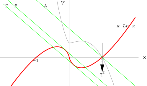
Figure 1: Graphical solution for Eq. (33). The thick curve represents the function $x\ln|x|$, the thin curve is the effective potential ${\cal V}$ at a given time, and the straight lines A, B, C represent the left hand side of (33) with $\Phi^{2}-\Phi_{R}^{2}=0,~{}\kappa-1-e^{-\kappa},~{}\kappa-1+e^{-\kappa}$ respectively, for $\kappa>1$. The arrow indicates how the lines move as $\Phi^{2}-\Phi_{R}^{2}$ increases. The potential has a local minimum at $x=0$.

As an explicit example, we consider $\kappa>1$ case in Fig. 1. The equation has three roots for $-\kappa+1+e^{-\kappa}<\Phi^{2}-\Phi_{R}^{2}<-(-\kappa+1+e^{-\kappa})$, two roots for $\Phi^{2}-\Phi_{R}^{2}=\pm(-\kappa+1+e^{-\kappa})$, and one root otherwise. For $\Phi^{2}-\Phi_{R}^{2}=(\kappa-1)$, the straight line passes through the origin. Note also that $\Phi^{2}-\Phi_{R}^{2}$ should be greater than $-\Phi_{R}^{2}$. The improvements in this solution from the previous works are the following: First, we always have roots of Eq. (33) for any value of $\bar{q}^{2}\geq 0$. Second, $x=0$ is not a special point now since the potential is continued for negative $x$.

The divergent part of the effective Hamiltonian (15) consists of two parts: $\displaystyle\frac{1}{2}\mu^{2}q^{2}-\frac{\lambda}{8}\left(\int_{\bf k}\phi^{*}_{\bf k}\phi_{\bf k}\right)^{2}$ and $\int_{\bf k}H_{G,\bf k}$. It is convenient to change the first part using Eq. (31) to give

$$\frac{1}{2}\mu^{2}q^{2}-\frac{\lambda}{8}\left(\int_{\bf k}G_{\bf k}\right)^{2}=\frac{\mu^{2}}{2}\bar{q}^{2}+\frac{m^{2}}{2}(q^{2}-\bar{q}^{2})-\frac{\lambda}{8}I_{0}^{2}(m^{2})+\frac{\lambda}{2}\bar{q}^{2}(q^{2}-\bar{q}^{2}),$$ (34)

where the divergences in $I_{0}^{2}$ and bare mass, $\mu^{2}$, are separated from the finite contributions. If one incorporates the renormalization condition (29), the last term in Eq. (34) goes to zero since the bare coupling is $-0$. In the second part, we separate the time-dependent part from time-independent part using the explicit formula for $G_{\bf k}$, Eq. (28),

$$\int_{\bf k}H_{G,\bf k}=\theta(-x)\bar{m}^{4}V_{L}(\bar{m},t)+\frac{1}{2}\int_{+,\bf k}\omega_{\bf k}=\theta(-x)\bar{m}^{4}V_{L}(\bar{m},t)+I_{1}(m^{2}),$$ (35)

where the time-dependent part is

$$V_{L}(\bar{m},t)=-\frac{4}{\bar{m}^{4}}\int_{|{\bf k}|<\bar{m}}(c_{1\bf k}c_{2\bf k}^{*}+c_{1\bf k}^{*}c_{2\bf k})\tilde{\omega}_{\bf k}+\frac{1}{\bar{m}^{4}}\int_{|{\bf k}|<\bar{m}}\left[\frac{1}{8}+(c_{1\bf k}c^{*}_{2\bf k}+c_{1\bf k}^{*}c_{2\bf k})^{2}\right]G_{\bf k}^{-1}.$$ (36)

Ignoring terms which go to zero when $\lambda\rightarrow-0$, we get the effective Hamiltonian

$$H_{eff}(q,p) = \frac{p^{2}}{2}+\frac{m^{2}}{2}(q^{2}-\bar{q}^{2})+\frac{\mu^{2}}{2}\bar{q}^{2}+I_{1}(m^{2})-\frac{\lambda}{8}I_{0}^{2}(m^{2})+\theta(-x)m_{R}^{4}x^{2}V_{L}(\bar{m},t)$$

$$= \frac{p^{2}}{2}+\frac{m^{2}}{2}(q^{2}-\bar{q}^{2})+\theta(-x)m_{R}^{4}x^{2}V_{L}(\bar{m},t)+V_{D}(\bar{q},m^{2}),$$

where the divergent part, $V_{D}$, becomes

$$V_{D}(\bar{q},m^{2}) = \frac{\mu^{2}}{2}\bar{q}^{2}+I_{1}(m^{2})-\frac{\lambda}{8}I_{0}^{2}(m^{2})$$

$$= D+\frac{\mu^{2}}{2}[\bar{q}^{2}-\bar{q}_{R}^{2}]+I_{1}(m^{2})-I_{1}(m_{R}^{2})-\frac{\lambda}{8}[I_{0}(m^{2})-I_{0}(m_{R}^{2})]$$

$$= \left\{\begin{tabular}[]{ll}$\displaystyle D+\frac{1}{2}m_{R}^{2}x(\bar{q}^{2}-\bar{q}_{R}^{2})+\frac{m_{R}^{4}}{32\pi^{2}}L_{3}(x)-\frac{m_{R}^{4}}{2\lambda_{R}}(x-1)^{2}$ ,&~{}~{}$\displaystyle x=\frac{m^{2}}{m_{R}^{2}}>0$ ,\\ $\displaystyle D+\frac{1}{2}m_{R}^{2}x(\bar{q}^{2}-\bar{q}_{R}^{2})+\frac{m_{R}^{4}}{32\pi^{2}}[L_{3}(-x)+2x]-\frac{m_{R}^{4}}{2\lambda_{R}}(x-1)^{2}$ ,&~{}~{} $\displaystyle x=\frac{m^{2}}{m_{R}^{2}}<0$,\end{tabular}\right.$$ (41)

with $\displaystyle D=\frac{\mu^{2}}{2}\bar{q}_{R}^{2}+I_{1}(m_{R}^{2})-\frac{\lambda}{8}I_{0}^{2}(m_{R}^{2})$ being a $q$ independent divergent constant. Let us define the normalized effective Hamiltonian by

$${\cal H} \equiv \frac{H_{eff}-D}{m_{R}^{4}/(64\pi^{2})}=64\pi^{2}\theta(-x)x^{2}V_{L}(\bar{m},t)+\frac{32\pi^{2}p^{2}}{m_{R}^{4}}+\frac{32\pi^{2}q^{2}}{m_{R}^{2}}x-2x\Phi_{R}^{2}+2L_{3}(|x|)+4x\theta(-x)-\kappa(x-1)^{2}$$

$$= \frac{32\pi^{2}p^{2}}{m_{R}^{4}}+\theta(-x)\left[64\pi^{2}x^{2}V_{L}(\bar{m},t)-\frac{32\pi^{2}x}{m_{R}^{2}}\int_{|{\bf k}|<\bar{m}}G_{\bf k}\right]+x(\Phi^{2}-\Phi_{R}^{2})-\frac{1}{2}(x-1)(x-1+2\kappa)$$

$$= \frac{32\pi^{2}p^{2}}{m_{R}^{4}}+\theta(-x)\left[64\pi^{2}x^{2}V_{L}(\bar{m},t)-\frac{32\pi^{2}x}{m_{R}^{2}}\int_{|{\bf k}|<\bar{m}}G_{\bf k}\right]-x^{2}\ln|x|+\left(\frac{1}{2}-\kappa\right)(x^{2}-1),$$

where we write the Hamiltonian in several different forms using Eq. (33).

Let us consider the case where the initial value is given by $c_{2\bf k}=0$ and $c_{1\bf k}=c_{1}$, to present an explicit form of the effective potential. Then, $V_{L}(\bar{m},t)$ exponentially decreases to zero as time $t\rightarrow\infty$ and

$$\int_{|{\bf k}|<\bar{m}}G_{\bf k} = \frac{|c_{1}|^{2}}{4\pi^{2}}\int_{0}^{\bar{m}}\frac{k^{2}e^{2t\sqrt{\bar{m}^{2}-k^{2}}}}{\sqrt{\bar{m}^{2}-k^{2}}}dk=\frac{|c_{1}|^{2}}{4\pi^{2}}\int_{0}^{\bar{m}}e^{f(k^{2}/\bar{m}^{2})}dk$$ (43)

where the function $f$ is maximized at $\displaystyle{\bf k}^{2}=\frac{\bar{m}}{t}$, and the integral can be performed using the steepest descent method to give (See Appendix A):

$$\int_{|{\bf k}|<\bar{m}}G_{\bf k}\simeq\frac{|c_{1}|^{2}}{4\pi^{2}}\sqrt{\frac{\pi\bar{m}}{2t^{3}}}e^{2\bar{m}t-1/2}.$$ (44)

Therefore, the renormalized effective potential at a given large time $t$ becomes

$${\cal V}(x) = \left.{\cal H}\right|_{p=0}=8|c_{1}|^{2}x^{2}g(m_{R}(-x)^{1/2}t)\theta(-x)-x^{2}\ln|x|+\left(\frac{1}{2}-\kappa\right)(x^{2}-1),$$ (45)

where $\displaystyle g(y)=\sqrt{\frac{\pi}{y^{3}}}e^{2y-1/2}$. The renormalized potential is symmetric about $x=0$ if $c_{1}=0$. The first term of the effective potential (45) exponentially increases as time so that one cannot have a large negative mass-squared at a later time.

Figure 2: Typical form of the effective potential ${\cal V}$ at a given time $t$. The horizontal axis represents $\bar{q}$. The global minimum at the origin is at $q=0$ and the local minima at $\bar{q}\neq 0$ is the point of $\bar{q}$ which corresponds to $x=0$.

Now we discuss the shape of the effective potential as a function of $\bar{q}$ as seen in Fig. 2. Since $\bar{q}=q$ for $m^{2}>0$, this gives the effective potential for $q$ for positive mass-squared case. As can be seen in Fig. 1, there is at least one root $x$ for a given $\bar{q}$. In the case of two or three $x$ roots, the true $x$ values should be chosen such that it minimize the effective potential (45). Then the absolute minimum of the potential is at $\Phi^{2}=0$. The potential increases as a function of $\Phi^{2}$ until $\Phi^{2}-\Phi_{R}^{2}=e^{-\kappa}-1+\kappa$ where $x=e^{-\kappa}$. It then decreases until $\Phi^{2}-\Phi_{R}^{2}=\kappa-1$ where $x=0$, which is a local minima of the effective potential, and then it increases again. The metastable state corresponds to $x=0$ so the theory is massless at that point. The effect of the inclusion of the negative mass-squared modes becomes apparent for large $\bar{q}^{2}$, in which, the potential exponentially increases in time and the mass-squared is negative. This means, for a realistic system, that the modes with negative mass squared soon decays to positive stable modes since it needs infinite energy to keep the negative mode continually.

Some comments are in order. Due to the inclusion of negative modes the solutions to the equation (33) always exist. Stevenson stevenson found that the present technique is inadequate to find the effective potential for negative $\kappa$ for the following reason: At $x=1$, we should have $(m^{2},q^{2})=(m_{R}^{2},q_{R}^{2})$. There are two solution for $x$ to the Eq. (33) if $\kappa<0$ and the solution at $x=1$ corresponds to the larger potential value of the two. This does not obey the guiding principle which chooses the $x$ which gives lower potential value. To overcome this difficulty he used a rescaling of variables which maps $\kappa<0$ into $0<\kappa<1$. This is also the case for the example above.

IV Spinodal instability and finite smooth quench by controlling the mass-squared

In this section, we consider a finite smooth quench model, which was previously considered in Ref. spkim . The finite quench transition is described by a scalar field with the mass given by

$$m^{2}(t)=\frac{m_{i}^{2}-m_{f}^{2}}{2}-\frac{m_{i}^{2}+m_{f}^{2}}{2}\tanh\left(\frac{t}{\tau}\right),$$ (46)

where $m_{i}^{2}$ and $m_{f}^{2}$ are both positive definite. At earlier time, $t=-\infty$, the mass-squared has the initial value $m_{i}^{2}$ and at later time, $t=\infty$, the final value $-m_{f}^{2}$. Here $\tau$ measures the quench rate: the large $\tau$ implies that the mass changes slowly, whereas the small $\tau$ implies a rapid change of the mass-squared. In particular, the $\tau\rightarrow 0$ limit corresponds to the instantaneous change from $m_{i}^{2}$ to $-m_{f}^{2}$ at $t=0$. To find the Fock space for each mode one needs to solve the classical equation of motion

$$\ddot{\phi}_{\bf k}(t)+\left[{\bf k}^{2}+\frac{m_{i}^{2}-m_{f}^{2}}{2}-\frac{m_{i}^{2}+m_{f}^{2}}{2}\tanh\left(\frac{t}{\tau}\right)\right]\phi_{\bf k}(t)=0.$$ (47)

It should be noted that the long wavelength modes, $|{\bf k}|\leq m_{f}$, lead to the change in the sign of the frequency at later times $(t\gg\tau)$,

$$\omega_{\bf k}^{2}(t)={\bf k}^{2}-m_{f}^{2}<0,$$ (48)

and suffer from spinodal instability. Each long wavelength mode has a different quench time determined by $\omega_{\bf k}^{2}(t_{\bf k})=0$. The solution to Eq. (47) are found separately for stable modes and unstable modes. The stable modes $(k\geq m_{f})$ have the solution

$$\phi_{\bf k}(t)=\frac{1}{\sqrt{2\omega_{i,\bf k}}}e^{-i\omega_{i,\bf k}t}~{}_{2}F_{1}(-i\tau\omega_{+,\bf k},-i\tau\omega_{-,\bf k};1-i\tau\omega_{i,\bf k};-e^{2t/\tau}),$$ (49)

where

$$\omega_{\pm,\bf k}=\frac{\omega_{i,\bf k}\pm\omega_{f,\bf k}}{2},$$ (50)

with

$$\omega_{i,\bf k}=\sqrt{{\bf k}^{2}+m_{i}^{2}},~{}~{}\omega_{f,\bf k}=\sqrt{{\bf k}^{2}-m_{f}^{2}}.$$ (51)

Whereas the unstable modes $(|{\bf k}|<m_{f})$ have the solution

$$\phi_{\bf k}(t)=\frac{1}{\sqrt{2\omega_{i,\bf k}}}e^{-i\omega_{i,\bf k}t}~{}_{2}F_{1}(\tau w_{\bf k},-\tau w_{\bf k}^{*};1-i\tau\omega_{i,\bf k};-e^{2t/\tau}),$$ (52)

where the complex frequency is given by

$$w_{\bf k}=\frac{\tilde{\omega}_{f,\bf k}+i\omega_{i,\bf k}}{2}.$$ (53)

At earlier time $(t\ll-\tau)$ before the quench begins, both solutions (49) and (52) have the same asymptotic form

$$\phi_{i,\bf k}(t)=\frac{1}{\sqrt{2\omega_{i,\bf k}}}e^{-i\omega_{i,\bf k}t},$$ (54)

which matches the initial condition (14). At later time $(t\gg\tau)$ after the completion of quench, we find, by using the asymptotic form of the hypergeometric function GR , the asymptotic form for the stable modes (49)

$$\phi_{f_{S},{\bf k}}(t) = C_{S+,\bf k}\frac{e^{-i\omega_{f,\bf k}t}}{\sqrt{2\omega_{f,\bf k}}}+C_{S-,\bf k}\frac{e^{i\omega_{f,\bf k}t}}{\sqrt{2\omega_{f,\bf k}}},$$ (55)

where

$$C_{S\pm,\bf k}=\sqrt{\frac{\omega_{f,\bf k}}{\omega_{i,\bf k}}}\frac{\Gamma(1-i\omega_{i,\bf k}\tau)\Gamma(\mp i\omega_{f,\bf k}\tau)}{\Gamma(1-i\omega_{\pm,\bf k}\tau)\Gamma(-i\omega_{\pm,\bf k}\tau)},$$ (56)

and the asymptotic form for the unstable modes (52)

$$\phi_{f_{U},{\bf k}}(t) = C_{U+,\bf k}\frac{e^{\tilde{\omega}_{f,\bf k}t}}{\sqrt{2\tilde{\omega}_{f,\bf k}}}+C_{U-,\bf k}\frac{e^{-\tilde{\omega}_{f,\bf k}t}}{\sqrt{2\tilde{\omega}_{f,\bf k}}},$$ (57)

where

$$C_{U+,\bf k}=\sqrt{\frac{\tilde{\omega}_{f,\bf k}}{\omega_{i,\bf k}}}~{}\frac{\Gamma(1-i\omega_{i,\bf k}\tau)\Gamma(\tilde{\omega}_{f,\bf k}\tau)}{w_{\bf k}^{*}\tau\Gamma^{2}(w_{\bf k}^{*}\tau)},~{}~{}C_{U-,\bf k}=\sqrt{\frac{\tilde{\omega}_{f,\bf k}}{\omega_{i,\bf k}}}~{}\frac{\Gamma(1-i\omega_{i,\bf k}\tau)\Gamma(-\tilde{\omega}_{f,\bf k}\tau)}{-w_{\bf k}\tau\Gamma^{2}(-w_{\bf k}\tau)}.$$ (58)

From these results, the transition rate from the initial vacuum to the final vacuum and the coefficient of the negative frequency solution leading to the particle production rate were calculated in Ref. spkim . The asymptotic form for $\phi_{fU,\bf k}^{*}\phi_{fU,\bf k}$ was also calculated to obtain the scaling relation of the domain size

$$\xi_{D}(t)=\sqrt{\frac{8\tilde{t}}{m_{f}}},$$ (59)

where

$$\tilde{t}=t-\frac{\tau^{3}}{2}[\zeta(3)-1]|w_{\bf k}|^{2}.$$ (60)

For use in the next section, we explicitly present some more results not mentioned in Ref. spkim . The asymptotic form of the absolute square of the stable modes are

$$G_{f_{S},\bf k}=\phi_{f_{S},\bf k}^{*}(t)\phi_{f_{S},\bf k}(t) = \frac{g^{+}_{\bf k}}{2\omega_{f,\bf k}}\left[1+R^{+}_{\bf k}\cos\left(2\omega_{f,\bf k}t-\psi^{+}_{\bf k}\right)\right],$$ (61)

with the time-independent constants $g_{\bf k}^{+}$, $R_{\bf k}^{+}$, and $\psi_{\bf k}^{+}$ given by

$$g^{+}_{\bf k} = \frac{\sinh^{2}\pi\omega_{+,\bf k}\tau+\sinh^{2}\pi\omega_{-,\bf k}\tau}{\sinh\pi\omega_{i,\bf k}\tau\sinh\pi\omega_{f,\bf k}\tau}$$ (62)

$$R^{+}_{\bf k} = \left[\frac{\sinh\pi\omega_{+,\bf k}\tau}{\sinh\pi\omega_{-,\bf k}\tau}+\frac{\sinh\pi\omega_{-,\bf k}\tau}{\sinh\pi\omega_{+,\bf k}\tau}\right]^{-1},$$ (63)

$$i\psi^{+}_{\bf k} = \ln\frac{\Gamma(1-i\omega_{f,\bf k}\tau)\Gamma(1+i\omega_{+,\bf k}\tau)\Gamma(1-i\omega_{-,\bf k}\tau)}{\Gamma(1+i\omega_{f,\bf k}\tau)\Gamma(1-i\omega_{+,\bf k}\tau)\Gamma(1+i\omega_{-,\bf k}\tau)},$$ (64)

where $\psi_{\bf k}^{+}=0$ for $|{\bf k}|\ll 1/\tau$, and $g_{\bf k}^{+}=1$, $R_{\bf k}^{+}=0$ for $|{\bf k}|\gg 1/\tau$. On the other hand, the ultra violet limit of $\phi_{f_{S},\bf k}^{*}(t)\phi_{f_{S},\bf k}(t)$ is given by

$$G_{f_{S},\bf k}(t)=\frac{1}{2\omega_{f,\bf k}}+O(e^{-\pi\omega_{i,\bf k}\tau}),~{}~{}{\bf k}^{2}\gg\frac{1}{\tau^{2}}.$$ (65)

Using the properties of $\Gamma$ functions we get the instantaneous quench limit ($\tau\rightarrow 0$) of the stable modes and the unstable modes:

$$\lim_{\tau\rightarrow 0}\phi_{f_{S},\bf k}(t) = \frac{1}{2\sqrt{2\omega_{f,\bf k}}}\left[\left(\sqrt{\frac{\omega_{f,\bf k}}{\omega_{i,\bf k}}}+\sqrt{\frac{\omega_{i,\bf k}}{\omega_{f,\bf k}}}\right)e^{-i\omega_{f,\bf k}t}+\left(\sqrt{\frac{\omega_{f,\bf k}}{\omega_{i,\bf k}}}-\sqrt{\frac{\omega_{i,\bf k}}{\omega_{f,\bf k}}}\right)e^{i\omega_{f,\bf k}t}\right],$$ (66)

$$\lim_{\tau\rightarrow 0}\phi_{f_{U},\bf k}(t) = \frac{1}{2\sqrt{2\omega_{f,\bf k}}}\left[\left(\sqrt{\frac{\omega_{f,\bf k}}{\omega_{i,\bf k}}}-i\sqrt{\frac{\omega_{i,\bf k}}{\omega_{f,\bf k}}}\right)e^{\omega_{f,\bf k}t}+\left(\sqrt{\frac{\omega_{f,\bf k}}{\omega_{i,\bf k}}}+i\sqrt{\frac{\omega_{i,\bf k}}{\omega_{f,\bf k}}}\right)e^{-\omega_{f,\bf k}t}\right],$$ (67)

and their absolute squares are

$$\lim_{\tau\rightarrow 0}G_{f_{S},\bf k}(t) = \frac{1}{2\omega_{f,\bf k}}\left(\Omega_{+,\bf k}-\Omega_{-,\bf k}\cos 2\omega_{f,\bf k}t\right),$$ (68)

$$\lim_{\tau\rightarrow 0}G_{f_{U},\bf k}(t) = \frac{1}{2\tilde{\omega}_{f,\bf k}}\left(\tilde{\Omega}_{-,\bf k}+\tilde{\Omega}_{+,\bf k}\cosh 2\tilde{\omega}_{f,\bf k}t\right),$$ (69)

where

$$\Omega_{\pm,\bf k}=\frac{1}{2}\left(\frac{\omega_{f,\bf k}}{\omega_{i,\bf k}}\pm\frac{\omega_{i,\bf k}}{\omega_{f,\bf k}}\right),~{}~{}\tilde{\Omega}_{\pm,\bf k}=\frac{1}{2}\left(\frac{\tilde{\omega}_{f,\bf k}}{\omega_{i,\bf k}}\pm\frac{\omega_{i,\bf k}}{\tilde{\omega}_{f,\bf k}}\right).$$ (70)

All of these limiting properties are used in the next section to obtain the WKB mode solutions with arbitrary time-dependent mass.

V Time evolution and renormalization of a system after instantaneous quenching

The model described in Sec IV does not describe a real system undergoing second order phase transition because the spinodal instability increases indefinitely. This model describes an intermediate process of the realistic phase transition toward the spinodal line, $m^{2}(t_{k})={\bf k}^{2}$, at which point the instability of the mode $\phi_{\bf k}$ stops to increase. In this section we consider a self-interacting scalar field model by properly treating the back-reaction of the field through the $\lambda\phi^{4}$ interaction. All the instabilities end to increase at time ${\cal T}$ defined by $m^{2}({\cal T})=0$. Let the mass-squared of the scalar field $m^{2}(t)$ be positive value $m_{i}^{2}$ for $t<0$ and then it suddenly jumps to negative value $-m_{f}^{2}$ at $t=\tau\ll m_{i}^{-1}$. We consider the quench to occur in time $\tau$ which is far smaller than the normal time scale ($1/m$), which is why we use the word “instantaneous” even though it is not zero. And the time $\tau$ should not be zero since no realistic physical processes can alter the mass-squared instantaneously. Unlike the example in the previous section, we do not keep the mass-squared, $m^{2}(t)$, fixed, instead we let the mass-squared vary freely by self interaction after the quench $t>\tau$. The self-interaction of the scalar field leads to the gradually increasing mass-squared to a positive value as time.

The equation of motion for the mode solution (11), then, becomes

$$\ddot{\phi}_{\bf k}(t)+[{\bf k}^{2}+m^{2}(t)]\phi_{\bf k}(t)=0.$$ (71)

Since the mass-squared is negative at $t=\tau$, the modes for $t\geq\tau$ are divided into two categories depending on the size of momentum relative to the mass

$$\phi_{\bf k}(t)=\left\{\begin{tabular}[]{ll}$\displaystyle\phi_{\bf k}^{U}$,&~{}~{}~{}${\bf k}^{2}\leq-m^{2}(t)$,\vspace{.1cm}\\ $\displaystyle\phi_{\bf k}^{S}$,&~{}~{}~{}${\bf k}^{2}>-m^{2}(t)$.\\ \end{tabular}\right.$$ (74)

In the WKB approximation, the unstable mode, $\phi^{U}_{\bf k}$, has exponential type solution and the stable mode, $\phi^{S}_{\bf k}$, has oscillatory solution. Let us assume that $\omega_{\bf k}^{2}(t)={\bf k}^{2}+m^{2}(t)$ increases for $t>\tau$ due to the back reactions. Then, the unstable mode, $\phi^{U}_{\bf k}$, becomes stable at time $t_{k}$, given by ${\bf k}^{2}+m^{2}(t_{k})=0$. Conversely, for a given time $t$ the modes $\phi^{U}_{\bf k}$ with $|{\bf k}|^{2}\leq-m^{2}(t)$ are unstable and the modes $\phi^{S}_{\bf k}$ with $|{\bf k}|^{2}>-m^{2}(t)$ are stable. Since the mass-squared increases as time, the number of unstable modes decreases and finally the unstable modes disappear at time ${\cal T}$, where $m^{2}({\cal T})=0$, which means the ending of the instability growth. Now, the dynamical process can be divided into three cases depending on the regions of time. First is the time before the transition $t<0$ which is given by the initial condition, second is the spinodal development process, $0<t<{\cal T}$, the phase transition, and the final one is the stabilization process after the termination of the instability growth, $t>{\cal T}$.

Let us assume $q(t)=0$ and $m^{2}(t)=m_{i}^{2}>0$ for $t<0$. Then, the initial state becomes

$$\phi_{\bf k}(t<0)=\frac{1}{\sqrt{2\omega_{i,{\bf k}}}}e^{-i\omega_{i,{\bf k}}t},$$ (75)

and Eq. (12) yields the gap equation

$$\omega_{i,{\bf k}}^{2}=m_{i}^{2}+{\bf k}^{2}=\mu_{i}^{2}+{\bf k}^{2}+\frac{\lambda\hbar}{2}\int_{\bf k}\frac{1}{2\omega_{i,{\bf k}}}\coth\left(\frac{\beta\omega_{i,{\bf k}}}{2}\right),$$ (76)

where $\mu_{i}$ is the initial bare mass and $\lambda$ is the bare coupling. The infinities in the ${\bf k}$ integral are absorbed into the bare mass and the bare coupling leading to finite and positive $m_{i}^{2}$. For convenience we use the notation $\tilde{\omega}^{2}_{\bf k}(t)=-\omega^{2}_{\bf k}(t)\geq 0$ for the modes ${\bf k}^{2}\leq-m^{2}(t)$;

$$\tilde{\omega}_{\bf k}^{2}(t)=\bar{m}^{2}(t)-{\bf k}^{2}=-\mu^{2}(t)-{\bf k}^{2}-\frac{\lambda}{2}\int_{k}\phi_{\bf k}^{*}(t)\phi_{\bf k}(t)\coth\left(\frac{\beta\omega_{i,{\bf k}}}{2}\right)\geq 0.$$ (77)

Using Eq. (66) and the WKB approximation of Eq. (71), we get the solution for a given time $t>\tau$,

$$\phi_{\bf k}^{U}(t) = C_{U+,\bf k}\frac{e^{\int_{0}^{t}\tilde{\omega}_{\bf k}(t^{\prime})dt^{\prime}}}{\sqrt{2\tilde{\omega}_{\bf k}(t)}}+C_{U-,\bf k}\frac{e^{-\int_{0}^{t}\tilde{\omega}_{\bf k}(t^{\prime})dt^{\prime}}}{\sqrt{2\tilde{\omega}_{\bf k}(t)}},~{}~{}~{}~{}0\leq{\bf k}^{2}<-m^{2}(t),$$ (78)

$$\phi_{\bf k}^{S}(t) = \left\{\begin{tabular}[]{ll}$\displaystyle C_{U+,\bf k}\phi_{U,\bf k}^{+}-C_{U-,\bf k}\phi_{U,\bf k}^{-},$&~{}~{} $-m^{2}(t)\leq{\bf k}^{2}<m_{f}^{2},$\vspace{.1cm}\\ $\displaystyle C_{S+,\bf k}\frac{e^{-i\int_{0}^{t}\omega_{\bf k}(t^{\prime})dt^{\prime}}}{\sqrt{2\omega_{\bf k}(t)}}+C_{S-,\bf k}\frac{e^{i\int_{0}^{t}\omega_{\bf k}(t^{\prime})dt^{\prime}}}{\sqrt{2\omega_{\bf k}(t)}},$&~{}~{}$~{}~{}{\bf k}^{2}\geq m_{f}^{2}$,\end{tabular}\right.$$ (81)

where we use the matching condition,

$$\frac{1}{\sqrt{2\tilde{\omega}_{\bf k}(t)}}e^{-\int_{t}^{t_{k}}\tilde{\omega}_{\bf k}(t^{\prime})dt^{\prime}}~{} \longleftrightarrow ~{}\frac{\sqrt{2\pi}{\rm Ai}[-\mu_{k}(t-t_{k})]}{\mu_{k}^{1/2}}~{}\longleftrightarrow\phi^{+}_{U,\bf k}=\sqrt{\frac{2}{\omega_{\bf k}(t)}}\cos\left(\int_{t_{k}}^{t}\omega_{\bf k}(t^{\prime})dt^{\prime}-\frac{\pi}{4}\right),$$ (82)

$$\frac{1}{\sqrt{2\tilde{\omega}_{\bf k}(t)}}e^{\int_{t}^{t_{k}}\tilde{\omega}_{\bf k}(t^{\prime})dt^{\prime}}~{} \longleftrightarrow ~{}\sqrt{\frac{\pi}{2}}\frac{{\rm Bi}[-\mu_{k}(t-t_{k})]}{\mu_{k}^{1/2}}~{}\longleftrightarrow~{}\phi^{-}_{U,\bf k}=-\frac{1}{\sqrt{2\omega_{\bf k}(t)}}\sin\left(\int_{t_{k}}^{t}\omega_{\bf k}(t^{\prime})dt^{\prime}-\frac{\pi}{4}\right),$$

of WKB approximation at time $t=t_{k}$, where $\displaystyle\mu_{k}=\left[\frac{dm^{2}}{dt}(t_{k})\right]^{1/3}$, and ${\rm Ai}(x)$ and ${\rm Bi}(x)$ are the Airy functions. Later in this paper, we use the notation

$$\tilde{\theta}_{\bf k}(t)=\int_{0}^{t}\tilde{\omega}_{\bf k}(t^{\prime})dt^{\prime},~{}~{}~{}\theta^{+}_{\bf k}(t)=\int_{0}^{t}\omega_{\bf k}(t^{\prime})dt^{\prime},~{}~{}~{}\theta^{-}_{\bf k}(t)=\int_{t_{k}}^{t}\omega_{\bf k}(t^{\prime})dt^{\prime}.$$ (83)

In the case of the unstable modes, $|{\bf k}|<\bar{m}(t)$, the frequency satisfies $|{\bf k}|\tau\ll 1$, which leads to

$$\phi_{\bf k}^{U}(t) = \frac{1}{2\sqrt{2\tilde{\omega}_{\bf k}(t)}}\left[\left(\sqrt{\frac{\tilde{\omega}_{f,\bf k}}{\omega_{i,\bf k}}}-i\sqrt{\frac{\omega_{i,\bf k}}{\tilde{\omega}_{f,\bf k}}}\right)e^{\tilde{\theta}_{\bf k}(t)}+\left(\sqrt{\frac{\tilde{\omega}_{f,\bf k}}{\omega_{i,\bf k}}}+i\sqrt{\frac{\omega_{i,\bf k}}{\tilde{\omega}_{f,\bf k}}}\right)e^{-\tilde{\theta}_{\bf k}(t)}\right].$$ (84)

Therefore the WKB extended stable mode $\phi^{S}_{\bf k}(t)$ for $-m^{2}(t)<{\bf k}^{2}\leq m_{f}^{2}$ becomes

$$\phi^{S}_{\bf k}(t)=\frac{1}{2}\left(\sqrt{\frac{\tilde{\omega}_{f,\bf k}}{\omega_{i,\bf k}}}-i\sqrt{\frac{\omega_{i,\bf k}}{\tilde{\omega}_{f,\bf k}}}\right)e^{\tilde{\theta}_{\bf k}(t_{k})}\phi^{+}_{U,\bf k}(t)+\frac{1}{2}\left(\sqrt{\frac{\tilde{\omega}_{f,\bf k}}{\omega_{i,\bf k}}}+i\sqrt{\frac{\omega_{i,\bf k}}{\tilde{\omega}_{f,\bf k}}}\right)e^{-\tilde{\theta}_{\bf k}(t_{k})}\phi^{-}_{U,\bf k}(t).$$ (85)

Similarly, the stable modes with moderate frequencies $(m_{f}\leq|{\bf k}|\ll 1/\tau)$ become

$$\phi_{\bf k}^{S}(t) = \frac{1}{2\sqrt{2\omega_{\bf k}(t)}}\left[\left(\sqrt{\frac{\omega_{f,\bf k}}{\omega_{i,\bf k}}}+\sqrt{\frac{\omega_{i,\bf k}}{\omega_{f,\bf k}}}\right)e^{-i\theta^{+}_{\bf k}(t)}+\left(\sqrt{\frac{\omega_{f,\bf k}}{\omega_{i,\bf k}}}-\sqrt{\frac{\omega_{i,\bf k}}{\omega_{f,\bf k}}}\right)e^{i\theta^{+}_{\bf k}(t)}\right],$$ (86)

and the stable modes with very high frequencies $(|{\bf k}|\gg 1/\tau)$ become

$$\phi^{S}_{\bf k}(t)=\frac{\omega_{i,\bf k}^{-i\omega_{i,\bf k}\tau}\omega_{f,\bf k}^{-i\omega_{f,\bf k}\tau}}{\omega_{+,\bf k}^{-2i\omega_{+,\bf k}\tau}}\frac{e^{-i\theta^{+}_{\bf k}(t)}}{\sqrt{2\omega_{\bf k}(t)}}+O(e^{-\pi\omega_{i,\bf k}\tau}).$$ (87)

As shown in Eqs. (86) and (87) the UV behavior of the stable modes takes different form depending on the value of the large momentum compared to $1/\tau$.

The absolute square of this mode solution, $G_{\bf k}(t)=\phi_{\bf k}^{*}(t)\phi_{\bf k}(t)$, can be written as

$$G^{U}_{\bf k}(t) = \frac{1}{2\tilde{\omega}_{\bf k}(t)}\left[\tilde{\Omega}_{-,\bf k}+\tilde{\Omega}_{+,\bf k}\cosh 2\tilde{\theta}_{\bf k}(t)\right],{\bf k}^{2}<-m^{2}(t),$$ (88)

$$G^{S}_{\bf k}(t) = \left\{\begin{tabular}[]{ll}$\displaystyle\frac{g^{-}_{\bf k}}{2\omega_{\bf k}(t)}\left[1+R^{-}_{\bf k}\cos\left(2\theta^{-}_{\bf k}(t)-\psi^{-}_{\bf k}\right)\right]$,&~{}~{}$-m^{2}(t)<{\bf k}^{2}\leq m_{f}^{2}$\\ $\displaystyle\frac{g^{+}_{\bf k}}{2\omega_{\bf k}(t)}\left[1+R^{+}_{\bf k}\cos\left(2\theta^{+}_{\bf k}(t)-\psi^{+}_{\bf k}\right)\right]$&,~{}~{}${\bf k}^{2}\geq m_{f}^{2}$,\\ \end{tabular}\right.$$ (91)

where $g^{+}_{\bf k}$, $R^{+}_{\bf k}$, and $\theta^{+}_{\bf k}$ are given in Eq. (62), and

$$g^{-}_{\bf k} = \tilde{\Omega}_{+,\bf k}\left[e^{2\tilde{\theta}_{\bf k}(t_{k})}+\frac{1}{4}e^{-2\tilde{\theta}_{\bf k}(t_{k})}\right],$$ (92)

$$R^{-}_{\bf k} = \left[\left(\frac{e^{4\tilde{\theta}_{\bf k}(t_{k})}-1/4}{e^{4\tilde{\theta}_{\bf k}(t_{k})}+1/4}\right)^{2}+\left(\frac{\tilde{\Omega}_{-,\bf k}}{\tilde{\Omega}_{+,\bf k}}\right)^{2}\frac{16}{\left(4e^{2\tilde{\theta}_{\bf k}(t_{k})}+e^{-2\tilde{\theta}_{\bf k}(t_{k})}\right)^{2}}\right]^{1/2},$$ (93)

$$\tan\psi^{-}_{\bf k} = \frac{\tilde{\Omega}_{+,\bf k}}{\tilde{\Omega}_{-,\bf k}}\left[e^{2\tilde{\theta}_{\bf k}(t_{k})}-\frac{1}{4}e^{-2\tilde{\theta}_{\bf k}(t_{k})}\right].$$ (94)

Note also that $G^{S}_{\bf k}(t)$ in the UV limit ($|{\bf k}|\gg 1/\tau)$ is

$${\phi_{\bf k}^{S}}^{*}(t)\phi_{\bf k}^{S}(t)=\frac{1}{2\omega_{\bf k}(t)}+O(e^{-\pi\omega_{i,\bf k}\tau}).$$ (95)

On the other hand, in the intermediate region ($m_{f}\leq|{\bf k}|\ll 1/\tau$), it becomes

$${\phi_{\bf k}^{S}}^{*}(t)\phi_{\bf k}^{S}(t)=G_{\bf k}^{M}(t)\equiv\frac{1}{2\omega_{\bf k}(t)}\left[\Omega_{+,\bf k}+\Omega_{-,\bf k}\cos 2\theta^{+}_{\bf k}(t)\right],~{}~{}m_{f}\leq|{\bf k}|\ll 1/\tau.$$ (96)

Note also that the time derivatives of $G$’s satisfy

$$\dot{G}^{U}_{\bf k}(t) = \frac{\dot{m^{2}}}{2\tilde{\omega}_{\bf k}^{2}}G^{U}_{\bf k}(t)+\tilde{\Omega}_{+,\bf k}\sinh 2\tilde{\theta}_{\bf k}(t),$$ (97)

$$\dot{G}^{S}_{\bf k}(t) = -\frac{\dot{m^{2}}(t)}{2\omega^{2}_{\bf k}(t)}G^{S}_{\bf k}(t)-g^{\pm}_{\bf k}R^{\pm}_{\bf k}\sin\left[2\theta^{\pm}_{\bf k}(t)-\psi^{\pm}_{\bf k}\right].$$ (98)

Therefore, the $H_{\bf k}$ in Eq. (16) becomes

$$H^{S}_{\bf k} = \frac{(\dot{m^{2}})^{2}}{32\omega_{\bf k}^{4}}G_{\bf k}^{S}+\frac{\dot{m^{2}}}{8\omega_{\bf k}^{2}}g^{\pm}_{\bf k}R^{\pm}_{\bf k}\sin\left[2\theta^{\pm}_{\bf k}(t)-\psi^{\pm}_{\bf k}\right]+\frac{1}{2}g_{\bf k}^{\pm}\omega_{\bf k}+\frac{1}{8}\left[1-g_{\bf k}^{\pm 2}(1-R_{\bf k}^{\pm 2})\right](G_{\bf k}^{S})^{-1},$$ (99)

$$H^{U}_{\bf k} = \frac{(\dot{m^{2}})^{2}}{32\tilde{\omega}_{\bf k}^{4}}G_{\bf k}^{U}+\frac{\dot{m^{2}}}{8\tilde{\omega}_{\bf k}^{2}}\tilde{\Omega}_{+,\bf k}\sinh 2\tilde{\theta}_{\bf k}(t)+\tilde{\omega}_{\bf k}^{2}G^{U}_{\bf k}-\frac{1}{2}\tilde{\omega}_{\bf k}\tilde{\Omega}_{-,\bf k}.$$

where we can ignore the last term of (99) for ${\bf k}^{2}\geq m_{f}^{2}$ since $\displaystyle g_{\bf k}^{+2}(1-R_{\bf k}^{+2})=\left[\frac{\sinh^{2}\pi\omega_{+,\bf k}\tau-\sinh^{2}\pi\omega_{-,\bf k}\tau}{\sinh\pi\omega_{f,\bf k}\tau\sinh\pi\omega_{i,\bf k}\tau}\right]^{2}\simeq 1$ for most range of $|{\bf k}|>\bar{m}$.

The ultra-violet divergences are related only to $\phi_{\bf k}^{S}$ modes. From the structure of $G^{S}_{\bf k}$ written in Eqs. (95) we see that the only divergence in $G^{S}_{\bf k}$ comes from $1/[2\omega_{\bf k}(t)]$ term. It is already shown that the equation of motion for this form of $G_{\bf k}$ is UV renormalizable pi1 ; kim with the condition given in (29). Using Eqs. (34) and (99), we get the effective Hamiltonian

$$H=H_{f}+\frac{1}{2}\mu^{2}\bar{q}^{2}+I_{1}(m^{2})-\frac{\lambda}{8}I_{0}^{2}(m)+\frac{1}{2}\int_{+,\bf k}(g_{\bf k}^{\pm}-1)\omega_{\bf k}$$ (100)

where

$$H_{f} = \frac{1}{2}\dot{q}^{2}+\frac{1}{2}m^{2}(t)[q^{2}(t)-\bar{q}^{2}(t)]+\frac{\lambda}{2}\bar{q}^{2}(q^{2}-\bar{q}^{2})+\frac{\lambda}{4!}q^{4}+(\dot{m^{2}})^{2}\int_{{\bf k}}\frac{G_{\bf k}}{32\omega_{\bf k}^{4}}$$

$$+ \frac{\dot{m^{2}}}{8}\left\{\int_{+,{\bf k}}\frac{g_{\bf k}^{\pm}R_{\bf k}^{\pm}}{\omega_{\bf k}^{2}}\sin\left[2\theta^{+}_{\bf k}(t)-\psi_{\bf k}^{\pm}\right]+\int_{{\bf k}^{2}<-m^{2}}\frac{\tilde{\Omega}_{+,\bf k}}{\tilde{\omega}_{\bf k}^{2}}\sinh 2\tilde{\theta}_{\bf k}(t)\right\}+\int_{{\bf k}^{2}<-m^{2}}\tilde{\omega}_{\bf k}^{2}G^{U}_{\bf k}-\frac{1}{2}\int_{{\bf k}^{2}<-m^{2}}\tilde{\omega}_{\bf k}\tilde{\Omega}_{-,\bf k}$$

$$+ \frac{1}{8}\int_{+,\bf k}\left[1-g_{\bf k}^{\pm 2}(1-R_{\bf k}^{\pm 2})\right](G_{\bf k}^{S})^{-1}.$$

The $\pm$ sign in $g^{\pm}_{\bf k}$, $R^{\pm}_{\bf k}$, and $\theta_{\bf k}^{\pm}$ should be chosen by the sign of $|{\bf k}|-m_{f}$. The large momentum expansion of $g_{\bf k}^{+}-1$ becomes

$$g_{\bf k}^{+}-1=\left\{\begin{tabular}[]{ll}$\displaystyle\frac{(\omega_{f,\bf k}-\omega_{i,\bf k})^{2}}{2\omega_{i,\bf k}\omega_{f,\bf k}}$,&~{}~{} $\bar{m}\leq|{\bf k}|\ll 1/\tau$,\vspace{.1cm}\\ $\displaystyle\frac{(m_{i}^{2}+m_{f}^{2})^{2}}{8\omega_{\bf k}^{4}(t)}+\cdots,$&~{}~{} $\bar{m}\ll|{\bf k}|\ll 1/\tau$,\vspace{.1cm}\\ $0$,&~{}~{} $|{\bf k}|\gg 1/\tau$ ,\\ \end{tabular}\right.$$ (105)

which gives a large contribution proportional to $\ln(m_{R}\tau)$ to the integral. This logarithmic contribution to the energy, which is related to the “instantaneous” quench process, changes the vacuum structure of the system in the sense that the transition probability from the initial vacuum to the final vacuum goes to zero in the $\tau\rightarrow 0$ limit. Since such zero-probability transition is not physical, we should restrict $\tau\neq 0$ so that the transition probability between the two vacuum does not vanish. Let us define the integral,

$$\bar{I}_{-1}(m^{2},m_{f}) \equiv \int_{m_{f}}^{1/\tau}\frac{k^{2}dk}{4\pi^{2}\omega_{\bf k}^{3}}$$

$$= \frac{1}{4\pi^{2}}\left[-\ln m_{f}\tau-(1+\bar{m}^{2}\tau^{2})^{-\frac{1}{2}}+\left(1+\frac{\bar{m}^{2}}{m_{f}^{2}}\right)^{-1/2}+\ln\frac{1+\sqrt{1+\bar{m}^{2}\tau}}{1+\sqrt{1+\bar{m}^{2}/m_{f}^{2}}}\right],$$

$$= \frac{1}{4\pi^{2}}\left[-\ln m_{f}\tau-1+\left(1+|x|/x_{f}\right)^{-1/2}-\ln\frac{1+\sqrt{1+|x|/x_{f}}}{2}\right],$$

where $x_{f}=m_{f}^{2}/m_{R}^{2}$, we ignored terms which vanish in the $\tau\rightarrow 0$ limit in the last equality, and we defined the integration range from $m_{f}$ to avoid the infra-red (IR) divergence which appear at the $k$ with $\omega_{\bf k}(t)=0$ if $m^{2}(t)<0$. We denote the finite part of the last integral in (100) by

$$V_{\tau}=\frac{1}{2}\int_{+,\bf k}(g_{\bf k}^{+}-1)\omega_{\bf k}(t)-\frac{(m_{i}^{2}+m_{f}^{2})^{2}}{8}\bar{I}_{-1}(m^{2},m_{f}).$$ (107)

Then, the Hamiltonian becomes

$$H=H_{f}+V_{\tau}+\frac{1}{2}\mu^{2}\bar{q}^{2}+I_{1}(m)-\frac{\lambda}{8}I_{0}^{2}(m)+\frac{(m_{i}^{2}+m_{f}^{2})^{2}}{8}\bar{I}_{-1}(m^{2},m_{f}),$$ (108)

where $H_{f}+V_{\tau}$ is the UV finite part of the Hamiltonian. Since the form of the divergences of the Hamiltonian is the same as Eq. (III), the renormalization can similarly be done:

$$H=D+H_{f}+V_{\tau}+\frac{m_{R}^{4}}{64\pi^{2}}\left[x(\Phi^{2}-\Phi_{R}^{2})-\frac{1}{2}(x-1)(x-1+2\kappa)\right]+\frac{(m_{i}^{2}+m_{f}^{2})^{2}}{8}\bar{I}_{-1}(m^{2},m_{f}),$$ (109)

where the divergent constant, $\displaystyle D=\frac{1}{2}\mu^{2}\bar{q}_{R}^{2}+I_{1}(m_{R})+\frac{\lambda}{8}I_{0}^{2}(m_{R})$. The last term in this Hamiltonian contains a large constant contribution, which is the energy added by the instantaneous quench at $t=0$.

If an observer is confined for $t>\tau$ and the experiments is done with the energy scale ${\bf k}^{2}\ll 1/\tau^{2}$, the experiments cannot probe the existence of the very high frequency behavior (95) of $G_{\bf k}$. In this case, one may do additional renormalization of the $\ln m_{R}\tau$ term which is related to the sudden change of the mass-squared at $t=0$,

$$H = D^{\prime}+H_{f}+V_{\tau}+\frac{m_{R}^{4}}{64\pi^{2}}{\cal V}_{vac},$$ (110)

$${\cal V}_{vac} = x(\Phi^{2}-\Phi_{R}^{2})-\frac{1}{2}(x-1)(x-1+2\kappa)+2(x_{i}+x_{f})^{2}\left[-1+\left(1+|x|/x_{f}\right)^{-1/2}-\ln\frac{1+\sqrt{1+|x|/x_{f}}}{2}\right],$$ (111)

where $x_{i}=m_{i}^{2}/m_{R}^{2}$, $x_{f}=m_{f}^{2}/m_{R}^{2}$, and $\displaystyle D^{\prime}=D-\frac{(m_{i}^{2}+m_{f}^{2})^{2}}{32\pi^{2}}\ln m_{f}\tau$. The divergence in $\bar{I}_{-1}(m^{2},m_{f})$ is the origin of the time-dependent renormalization, Eqs. (5.8) and (5.9) of Ref. boyanovsky . In some sense, ${\cal V}_{vac}$ denotes the vacuum structure since it comes from the UV behaviors of the mode solutions which will not be affected by small excitations of moderate modes. In this point of view, $H_{f}+V_{\tau}$ may be considered as an excitation to the vacuum state. It may be helpful to figure out the structure of the potential ${\cal V}_{vac}$. The new term ${\cal V}_{vac}-{\cal V}$ always decreases in $x$, which leads to the possibility of symmetry breaking. Since the mass-squared satisfies Eq. (30), the equation which determines $x$ by $\Phi$ is given by Eq. (33) and its solution is obtained by graphical method in Fig. 1.

Note also that in Eq. (31) the difference,

$$\bar{q}^{2}-q^{2}=\theta(-x)\int_{|{\bf k}|<\bar{m}}G^{U}_{\bf k}+\int_{+,\bf k}\frac{1}{2\omega_{\bf k}}\left[g_{\bf k}^{\pm}-1+g_{\bf k}^{\pm}R_{\bf k}^{\pm}\cos\left(2\theta^{\pm}_{\bf k}(t)-\psi_{\bf k}^{\pm}\right)\right]$$ (112)

is positive definite on time average due to Eq. (105). Therefore, the minimum value of $\bar{q}^{2}$ should be a positive number.

Note that the integral $\int_{\bf k}G_{\bf k}/\omega_{\bf k}^{4}$ in Eq. (V) is apparently IR divergent at the value of ${\bf k}$ where ${\bf k}^{2}+m^{2}=0$ if $m^{2}<0$. As one may see in the previous literatures pi1 ; kim , there is no IR divergence in the equations of motion expressed in $q$ and $G_{\bf k}$. Therefore, this IR divergences come from the approximation of $G_{\bf k}$ using the WKB solution. This origin of the IR divergence reminds us the validity range of the WKB approximation,

$$\left|\frac{\hbar\dot{m^{2}}(t)}{2\omega^{2}(t)}\right|\ll 1,$$ (113)

which clearly fails to be satisfied at “the classical point” $t=t_{k}$ where $\omega_{\bf k}^{2}(t_{k})=0$. In this sense, the IR divergence is the artifact of the WKB approximation around the transition point of $\omega_{\bf k}^{2}(t)$. The IR divergence does not have physical origin but comes from the bad choice of the solution of $\phi_{\bf k}$ near $t=t_{k}$. As an evidence of this argument, if one uses the exact solutions (Airy functions) near $t=t_{k}$, no divergences appear. To remedy this IR divergence, we need a generalized WKB approximation robicheaux , which is beyond the subject of this paper.

Fortunately and in fact naturally because this IR divergence comes from the failure of the WKB solution to satisfy the validity range of the WKB approximation (113), this IR divergences present only in the kinetic terms for $m^{2}(t)<0$, which do not influence the effective potential at a given time. The equations of motion which determine the $G_{\bf k}$ functions are also IR finite, which is related the physical correlation length. Moreover, the effective action after the termination of the spinodal transition, $t>{\cal T}$, is also IR finite. In the present paper we restrict our interest only to these cases.

VI Large instability approximation

In the last section, we renormalized the effective action and potential. In this section, we calculate the renormalized effective Hamiltonian and potential for the case ${\cal T}\gg 1/m$. The validity of this approximation should be checked by the dynamics at the time $\tau\leq t\leq{\cal T}$, which needs the full understanding of the IR properties mentioned at the end of the last section. In the absence of this knowledge, we can simply assume $m_{f}$ to be large and the renormalized coupling to be small so that it takes long enough time to increase the mass-squared to zero from $-m_{f}^{2}$. This approximation leads to the unstable modes to have large instability because of the exponential increase of the WKB solution, which is the reason we call it the large instability approximation.

Most part of this section is devoted to the evolution of the system at time $t>{\cal T}$ except for the short calculation of the effective potential for $m^{2}<0$ at the end of the this section. Therefore, the mass-squared is always positive definite and there is no unstable modes. The $G^{S}_{|{\bf k}|<m_{f}}$ function, in this approximation, is dominated by the exponentially growing term given by

$$G^{S}_{\bf k}(t)=\frac{\tilde{\Omega}_{+,\bf k}}{2\omega_{\bf k}(t)}e^{2\int_{0}^{t_{k}}\tilde{\omega}_{\bf k}(t^{\prime})dt^{\prime}}\left[1+\sin 2\theta^{-}_{\bf k}(t)\right],~{}~{}{\bf k}^{2}<m_{f}^{2},$$ (114)

and its integral over ${\bf k}$,

$$\int_{|{\bf k}|<m_{f}^{2}}G^{S}_{\bf k}(t)=\frac{1}{2\pi^{2}}\int_{0}^{m_{f}}dk\frac{\tilde{\Omega}_{+,\bf k}}{2\omega_{\bf k}(t)}\left[1+\sin 2\theta^{-}_{\bf k}(t)\right]e^{f(k^{2}/m_{f}^{2})},$$ (115)

is approximately integrated by using the steepest descent method in appendix B. The resulting integral formula are summarized in Eqs. (B) and (151). Before proceeding further, we define some parameters

$$\bar{l} = \left(\frac{m_{f}}{2\pi\alpha\bar{t}}\right)^{3/2}e^{2\tilde{\theta}_{\bar{k}}(\bar{t})},$$ (116)

$$\bar{k} = \left(\frac{m_{f}}{\alpha\bar{t}}\right)^{1/2},$$ (117)

$$\kappa = \bar{k}+i\bar{k}\Theta(t),$$ (118)

where $\bar{l}$ is a large scale which determines the instability, $1\leq\alpha\leq 2$ is a number, and $\bar{t}$ is a time scale determined by $\bar{k}^{2}+m^{2}(\bar{t})=0$, both of which are implicitly dependent on $\bar{k}$ and $\Theta(t)=\Theta(t,r=0)$ defined in Eq. (150).

We can approximate the integral in Eq. (115) as

$$\int_{|{\bf k}|<m_{f}}G^{S}_{\bf k}(t) \simeq \bar{l}\left\{\frac{\tilde{\Omega}_{+,\bar{k}}}{2\omega_{\bar{k}}(t)}+\frac{e^{-2\Theta^{2}(t)}}{4i}\left[\frac{\tilde{\Omega}_{+,\kappa}}{2\omega_{\kappa}(t)}e^{2i\theta^{-}_{\bar{k}}(t)}-\frac{\tilde{\Omega}_{+,\kappa^{*}}}{2\omega_{\kappa^{*}}(t)}e^{-2i\theta^{-}_{\bar{k}}(t)}\right]\right\}.$$ (119)

Therefore,

$$\bar{q}^{2}-q^{2}\simeq\bar{l}\left\{\frac{\tilde{\Omega}_{+,\bar{k}}}{2\omega_{\bar{k}}(t)}+\frac{e^{-2\Theta^{2}(t)}}{4i}\left[\frac{\tilde{\Omega}_{+,\kappa}}{2\omega_{\kappa}(t)}e^{2i\theta^{-}_{\bar{k}}(t)}-\frac{\tilde{\Omega}_{+,\kappa^{*}}}{2\omega_{\kappa^{*}}(t)}e^{-2i\theta^{-}_{\bar{k}}(t)}\right]\right\}+Q(m,t),$$ (120)

where $Q(m,t)=\int_{|{\bf k}|>m_{f}}G^{S}_{\bf k}(t)-I_{0}(m^{2})$, of which we present a rough estimation in appendix C. We do not need the full expression of $Q(m,t)$, rather it is enough to know that it behaves as $Q(m,t)\propto-m_{f}^{2}\sqrt{x/x_{f}}$ for large $x$.

Other integrals in Eq. (V) are given by

$$\int_{|{\bf k}|<m_{f}}\frac{G^{S}_{\bf k}(t)}{\omega_{\bf k}^{4}(t)}\simeq\bar{l}\left\{\frac{\tilde{\Omega}_{+,\bar{k}}}{2\omega_{\bar{k}}^{5}(t)}+\frac{e^{-2\Theta^{2}(t)}}{2i}\left[\frac{\tilde{\Omega}_{+,\kappa}}{2\omega_{\kappa}^{5}(t)}e^{2i\theta^{-}_{\bar{k}}(t)}-\frac{\tilde{\Omega}_{+,\kappa^{*}}}{2\omega_{\kappa^{*}}^{5}(t)}e^{-2i\theta^{-}_{\bar{k}}(t)}\right]\right\},$$ (121)

$$\int_{|{\bf k}|<m_{f}}\frac{g_{\bf k}^{-}R_{\bf k}^{-}}{\omega_{\bf k}^{2}(t)}\sin\left[2\theta^{-}_{\bf k}(t)-\psi_{\bf k}^{-}\right]\simeq-\bar{l}e^{-2\Theta^{2}(t)}\left[\frac{\tilde{\Omega}_{+,\kappa}}{2\omega_{\kappa}^{2}(t)}e^{2i\theta^{-}_{\bar{k}}(t)}+\frac{\tilde{\Omega}_{+,\kappa^{*}}}{2\omega_{\kappa^{*}}^{2}(t)}e^{-2i\theta^{-}_{\bar{k}}(t)}\right],$$ (122)

$$\frac{1}{8}\int_{+,\bf k}\left[1-g_{\bf k}^{\pm 2}(1-R_{\bf k}^{\pm 2})\right](G_{\bf k}^{S})^{-1}\simeq 0,$$ (123)

where in the second integral we use $\psi^{-}_{\bf k}\simeq\pi/2$, $g^{-}_{\bf k}\simeq\tilde{\Omega}_{+,\bf k}e^{2\tilde{\theta}_{\bf k}(t_{k})}$, and $R^{-}_{\bf k}\simeq 1$. We ignore the integrals $\displaystyle\int_{|{\bf k}|>m_{f}}\frac{G^{S}_{\bf k}(t)}{\omega_{\bf k}^{4}(t)}$ and $\displaystyle\int_{|{\bf k}|>m_{f}}\frac{g_{\bf k}^{-}R_{\bf k}^{-}}{\omega_{\bf k}^{2}(t)}\sin\left[2\theta^{-}_{\bf k}(t)-\psi_{\bf k}^{-}\right]$ compared to its small momentum term in Eq. (121).

Therefore, the $H_{f}$ becomes

$$H_{f} \simeq \frac{1}{2}\dot{q}^{2}+\frac{\bar{l}\tilde{\Omega}_{+,\bar{k}}}{4\omega_{\bar{k}}}\left[m^{2}+\frac{(\dot{m^{2}})^{2}}{16\omega_{\bar{k}}^{4}}\right]+\frac{1}{2}m^{2}Q(m,t)$$

$$+ \frac{\bar{l}e^{-2\Theta(t)^{2}}}{8}\left\{\frac{(\dot{m^{2}})^{2}}{8i}\left[\frac{\tilde{\Omega}_{+,\kappa}}{2\omega_{\kappa}^{5}(t)}e^{2i\theta^{-}_{\bar{k}}(t)}-\frac{\tilde{\Omega}_{+,\kappa^{*}}}{2\omega_{\kappa^{*}}^{5}(t)}e^{-2i\theta^{-}_{\bar{k}}(t)}\right]-\dot{m^{2}}\left[\frac{\tilde{\Omega}_{+,\kappa}}{2\omega_{\kappa}^{2}(t)}e^{2i\theta^{-}_{\bar{k}}(t)}+\frac{\tilde{\Omega}_{+,\kappa^{*}}}{2\omega_{\kappa^{*}}^{2}(t)}e^{-2i\theta^{-}_{\bar{k}}(t)}\right]\right.$$

$$- \left.im^{2}\left[\frac{\tilde{\Omega}_{+,\kappa}}{2\omega_{\kappa}(t)}e^{2i\theta^{-}_{\bar{k}}(t)}-\frac{\tilde{\Omega}_{+,\kappa^{*}}}{2\omega_{\kappa^{*}}(t)}e^{-2i\theta^{-}_{\bar{k}}(t)}\right]\right\}.$$

From Eq. (105) we know that the last integral is finite and small compared to the exponentiated terms. Similarly, the integral $\int_{|{\bf k}|>m_{f}}\frac{G_{\bf k}}{\omega_{\bf k}^{4}}$ can also be ignored compared to other terms.

We approximate $V_{\tau}$ also by its value around $k=m_{f}$. We should also calculate $\displaystyle\frac{1}{2}\int_{+,\bf k}g_{\bf k}^{-}\omega_{\bf k}$ in Eq. (100), which gives

$$V_{\tau}=\frac{\bar{l}}{2}\tilde{\Omega}_{+,\bar{k}}\omega_{\bar{k}}(t)+\frac{m_{f}^{4}}{32\pi^{2}}\left[\sqrt{1+\frac{x}{x_{f}}}\left(2+\frac{x}{x_{f}}\right)-\frac{x^{2}}{x_{f}^{2}}\ln\left(\sqrt{\frac{x_{f}}{x}}+\sqrt{1+\frac{x_{f}}{x}}\right)\right]+\frac{m_{f}^{4}g^{\prime}(x_{i},x_{f})}{32\pi^{2}}\sqrt{\frac{x}{x_{f}}+1},$$ (125)

where $g^{\prime}$ is a positive constant and the integrals needed in this equation is calculated in Appendix C.

One can sum everything to obtain $\displaystyle H_{eff}=D^{\prime}+H_{f}+V_{\tau}+\frac{m_{R}^{4}}{64\pi^{2}}{\cal V}_{vac}$. Before doing this summation, let us investigate where does the main contributions come from. Since $\omega_{\bar{k}}\simeq m(t)$, it is enough to observe the $m(t)$ dependence of each terms. The main contribution comes from the unstable modes which have $\bar{l}$ factor if the value of $x$ is not very large. For larger value of $x$ the $-x^{2}\ln|x|$ term in $V_{vac}$ starts to compete with $\bar{l}$ term and then dominates the potential for larger $x$. Therefore, to know the behavior of the effective Hamiltonian, we need to keep these terms only:

$$H_{eff}-D^{\prime} \simeq K+\frac{\bar{l}\tilde{\Omega}_{+,\bar{k}}}{2}\left[\omega_{\bar{k}}(t)+\frac{m^{2}(t)}{2\omega_{\bar{k}}(t)}\right]$$

$$+ \frac{\bar{l}m^{2}(t)e^{-2\Theta^{2}(t)}}{8i}\left[\frac{\tilde{\Omega}_{+,\kappa}}{2\omega_{\kappa}(t)}e^{2i\theta^{-}_{\bar{k}}(t)}-\frac{\tilde{\Omega}_{+,\kappa^{*}}}{2\omega_{\kappa^{*}}(t)}e^{-2i\theta^{-}_{\bar{k}}(t)}\right]-\frac{m_{R}^{4}}{64\pi^{2}}x^{2}\ln x,$$

where $K$ represents the sum of all kinetic terms and $\omega_{\bar{k}}/m_{R}=\sqrt{x+\bar{x}}$ with $\bar{x}=\bar{k}^{2}/m_{R}^{2}$. Therefore, the effective potential for very large $t$ and $x>0$ becomes

$${\cal V}=\frac{V_{eff}-D^{\prime}}{m_{R}^{4}/(64\pi^{2})} \simeq \frac{2v}{3}\left(\sqrt{x+\bar{x}}+\frac{x}{2\sqrt{x+\bar{x}}}\right)-x^{2}\ln x,$$ (127)

where $\displaystyle v=\frac{24\pi^{2}\bar{l}(x_{i}+x_{f})}{m_{R}^{3}\sqrt{x_{i}x_{f}}}$, and $\bar{x}\ll 1$ for large $\bar{t}$. Note that a natural stabilization of the effective potential occurs for large $t>{\cal T}$ due to the factor $e^{-2\Theta^{2}(t)}$.

Until now, we did not calculate the effective action for negative $x$ which is impossible until we treat the IR divergences properly, but the effective potential can still be calculable which exponentially increases in time as can be seen in Sec. III. The main contribution of the unstable modes comes from the integral $\int_{{\bf k}^{2}<-m^{2}}\tilde{\omega}_{\bf k}^{2}G^{U}_{\bf k}$ which becomes

$$\int_{{\bf k}^{2}<-m^{2}}\tilde{\omega}_{\bf k}^{2}G^{U}_{\bf k} \simeq \frac{1}{8\pi^{2}}\int_{0}^{\bar{m}}dk\tilde{\omega}_{\bf k}(t)\tilde{\Omega}_{+,\bf k}k^{2}e^{2\tilde{\theta}_{\bf k}(t)}$$

$$\simeq \frac{\tilde{\omega}_{{\bf k}_{t}}\tilde{\Omega}_{+,{\bf k}_{t}}}{4}\left(\frac{\pi{\bf k}_{t}^{2}}{2\pi}\right)^{3/2}e^{2\tilde{\theta}_{{\bf k}_{t}}(t)},$$

where $k_{t}$ is determined by $\displaystyle{\bf k}_{t}^{2}=\int_{0}^{t}dt^{\prime}\tilde{\omega}_{{\bf k}_{t}}^{-1}(t^{\prime})$. Due to the exponential factor in Eq. (VI), the potential (VI) for large $t$ is very sharply inclined to the vertical axis for negative $x$ so that $x$ increases. In summary, for a given time $t$, the effective potential for $x$ has minimum at $x=0$ and increases in both directions. For large $x\sim v^{2/3}$, the $x^{2}\ln x$ term starts to compete with $v\sqrt{x}$. For larger $x>v^{2/3}$, the potential starts to decrease. The relation between $\bar{q}^{2}-\bar{q}_{R}^{2}$ and $x$ is still determined by Eq. (33), whose solution is obtained by graphical method shown in Fig. 3 where the form of the potential is different from that in Fig. 1.

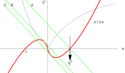
Figure 3: Graphical solution for Eq. (33). The thick curve represents the function $x\ln|x|$ and the thin curve represents the effective potential ${\cal V}/v$ (we set $v=50$ and $\bar{x}=1/4$ and normalize it so that it goes to zero at $x=0$.) at a given time, and the straight lines A, B, C represent the left hand side of (33) with $\Phi^{2}-\Phi_{R}^{2}=0,~{}\kappa-1-e^{-\kappa},~{}\kappa-1+e^{-\kappa}$, respectively, for $\kappa>1$. The arrow indicates how the lines move as $\Phi^{2}-\Phi_{R}^{2}$ increases. The potential has minimum at $x=0$.

With these we schematically plot the potential in $\bar{q}$ in Fig. 4,

Figure 4: Typical form of the effective potential ${\cal V}$ at a given time $t$. The horizontal axis is $\bar{q}$. The global minimum is at $\bar{q}\neq 0$ and $q=0$ is a local maximum.

which shows the presence of the symmetry breaking clearly. A few comments are in order. First, the potential is plotted as a function of $\bar{q}$. Since the minimum value of $\bar{q}$ corresponds to $q=0$, the form of the potential can roughly be interpreted as a potential for $q$ if $m^{2}>0$. On the other hand, if $m^{2}<0$, the relation between $\bar{q}$ and $q$ changes in time. Therefore, we should interpret the potential only at a given time. Second, the restriction $\kappa>0$ in the potential (45) disappears in the present case. Even for negative $\kappa$, the solution at $x=1$ corresponds to the smaller potential value of the two positive solution of (33) for large enough $v$.

All of the discussions in this section are the zero temperature results. The inclusion of non-zero initial temperature does not leads to a critical complication in the analysis. The only difference is that all the integrals in the calculations should contains the $\displaystyle\coth\frac{\beta\omega_{i,\bf k}}{2}$ factor. This results in the change of $\displaystyle\bar{l}\longrightarrow\bar{l}\coth\frac{\beta\omega_{i\bar{k}}}{2}$ for the unstable modes and the ${\cal V}$ in Eq. (45) becomes temperature dependent. However, these cannot alter the global behavior of the effective potential.

VII Equal time correlation function

Until now we have calculated the effective action with the precarious renormalization condition. However, the correlation function,

$$G({\bf x},{\bf y};t) = \int\frac{d^{3}{\bf k}}{(2\pi)^{3}}e^{i{\rm k}\cdot({\bf x-y})}G_{\bf k}(t)$$

$$= \frac{1}{2\pi^{2}r}\int kdk~{}\sin kr~{}G_{\bf k}(t)$$

$$\simeq \frac{1}{2\pi^{2}r}\left[\int_{0}^{\bar{m}}kdk~{}\sin kr~{}G^{U}_{\bf k}(t)+\int_{\bar{m}}^{m_{f}}kdk~{}\sin kr~{}G^{S}_{\bf k}(t)+\int_{m_{f}}^{\infty}kdk~{}\sin kr~{}G^{S}_{\bf k}(t)\right],$$

where $r=|{\bf x-y}|$, is renormalization scheme independent in the sense that the renormalization is related only to the stable modes and the dominant contribution to the correlation function comes from the exponential growth of the unstable modes. This observation enables one to ignore the last integral in Eq. (VII) which is related to the two point correlation function of stable system, which we ignore in this section compared to the first two integrals which contain exponentially increasing factors for large time.

Let us consider the first integral of Eq. (113) where the dominant part of the integrand is proportional to $k^{2}e^{2\tilde{\theta}_{\bf k}(t)}$, which is peaked around $\bar{k}$ where $\bar{k}^{-2}=\int_{0}^{t}dt^{\prime}\tilde{\omega}^{-1}_{\bar{k}}(t^{\prime})$. Then, the correlation function (VII) can be approximated by the contribution of the unstable mode $G^{U}$,

$$G^{U}({\bf x,y};t) = \frac{1}{2\pi^{2}}\int_{0}^{\bar{m}}k^{2}dk~{}\frac{\sin kr}{kr}~{}G^{U}_{\bf k}(t)\simeq\frac{1}{8\pi^{2}}\int_{0}^{\bar{m}}dk~{}\frac{\tilde{\Omega}_{+,\bf k}}{\tilde{\omega}_{\bf k}}k^{2}e^{2\tilde{\theta}_{\bf k}(t)}\frac{\sin kr}{kr}$$

$$\simeq \left(\frac{\bar{k}^{2}}{2\pi}\right)^{3/2}\exp\left[2\tilde{\theta}_{\bar{k}}(t)-\frac{\bar{k}^{2}r^{2}}{8}\right]\left[\frac{\tilde{\Omega}_{+,\kappa}}{\kappa\tilde{\omega}_{\kappa}}\frac{e^{i\bar{k}r}}{2ir}-\frac{\tilde{\Omega}_{+,\kappa^{*}}}{\kappa^{*}\tilde{\omega}_{\kappa^{*}}}\frac{e^{-i\bar{k}r}}{2ir}\right],$$

where $\displaystyle\kappa=\bar{k}+i\frac{r}{2\gamma}$. For large $t$, $\bar{k}/\bar{m}$ becomes very small, and the coefficient of $k^{2}e^{2\tilde{\theta}_{\bf k}(t)}$ should be smooth for small $k$. Another consequence of the small $\bar{k}$ is that the Gaussian integral well approximates $G^{U}$ for most range of $0<t<{\cal T}$, until $\bar{m}>\bar{k}$. This is why we approximate $k^{2}e^{2\tilde{\theta}_{\bf k}(t)}$ as a Gaussian function (the steepest descent method) factoring out the smooth function $\displaystyle\frac{\sin kr}{kr}$ in the integrand.

Let us consider the $r\rightarrow 0$ limit of this function,

$$\lim_{r\rightarrow 0}G^{U}({\bf x,y};t) = \left(\frac{\bar{k}^{2}}{2\pi}\right)^{3/2}\frac{e^{2\tilde{\theta}_{\bar{k}}(t)}}{4}\left[\frac{\tilde{\Omega}_{+,\bar{k}}}{\tilde{\omega}_{\bar{k}}}+\frac{1}{2}\lim_{r\rightarrow 0}\Im\frac{\tilde{\Omega}_{+,\kappa}}{r\kappa\tilde{\omega}_{\kappa}}\right]$$

$$= \frac{7}{8}\left(\frac{\bar{k}^{2}}{2\pi}\right)^{3/2}\frac{e^{2\tilde{\theta}_{\bar{k}}(t)}}{4}\frac{\tilde{\Omega}_{+,\bar{k}}}{\tilde{\omega}_{\bar{k}}}=\frac{7}{8}G^{U}({\bf x,x};t)=\frac{7}{8}G(0;t),$$

where in the last equality we use $\displaystyle\lim_{r\rightarrow 0}\Im\frac{\tilde{\Omega}_{+,\kappa}}{r\kappa\tilde{\omega}_{\kappa}}=\frac{1}{2\gamma}\frac{\partial}{\partial\bar{k}}\left(\frac{\tilde{\Omega}_{+,\bar{k}}}{\bar{k}\tilde{\omega}_{\bar{k}}}\right)\simeq-\frac{\tilde{\Omega}_{+,\bar{k}}}{\bar{k}^{2}\tilde{\omega}_{\bar{k}}}$. At $r=0$, this should correspond to $G^{U}({\bf x,x};t)=\int_{|{\bf k}|<\bar{m}}G_{\bf k}^{U}(t)$. Therefore in general we write

$$G({\bf x,y};0<t<{\cal T}) \simeq \frac{7}{16}G^{U}(0;t)\frac{\bar{\omega}_{\bar{k}}(t)}{\tilde{\Omega}_{+,\bar{k}}}\exp\left(-\frac{\bar{k}^{2}r^{2}}{8}\right)\left[\frac{\tilde{\Omega}_{+,\kappa}}{r\kappa\tilde{\omega}_{\kappa}(t)}e^{i\bar{k}r}-\frac{\tilde{\Omega}_{+,\kappa^{*}}}{r\kappa^{*}\tilde{\omega}_{\kappa^{*}}(t)}e^{-i\bar{k}r}\right],$$ (132)

where most of time-dependencies are given by $G^{U}(0;t)$ in Eq. (VII). Note that $1/\bar{k}^{2}\simeq 2\int_{0}^{t}dt^{\prime}\tilde{\omega}_{\bar{k}}^{-1}(t^{\prime})$ increases as time. The exponent $\bar{k}^{2}r^{2}/8$ determines the correlation length,

$$\xi_{D}(t)=2\sqrt{2}\left[\int_{0}^{t}dt^{\prime}\tilde{\omega}_{\bar{k}}^{-1}(t^{\prime})\right]^{1/2}\simeq 2\sqrt{2}\left[\int_{0}^{t}dt^{\prime}\tilde{m}^{-1}(t^{\prime})\right]^{1/2},$$ (133)

which gives the Cahn-Allen relation for constant $\bar{m}^{2}$, time lagged deformed relation $\displaystyle 4\left[\frac{1}{\alpha}\left(m_{f}-\sqrt{m_{f}^{2}-\alpha t}\right)\right]^{1/2}$ for linear mass-squared, $\bar{m}^{2}(t)=m_{f}^{2}-\alpha t$, which was discovered in Ref. spkim , and another deformed relation $\displaystyle 2\left[\frac{2}{\alpha}\tan^{-1}\frac{\alpha t}{\sqrt{m_{f}^{2}-\alpha^{2}t^{2}}}\right]^{1/2}$ for quadratic mass-squared $\bar{m}^{2}(t)=m_{f}^{2}-\alpha^{2}t^{2}$. Note that the last two deformed relations have the maxima of the correlation length given by $\displaystyle\sqrt{\frac{8m_{f}}{\alpha}}$ and $\displaystyle\sqrt{\frac{2\pi}{\alpha}}$, respectively. This is because the instability ends to increase at the time where $\bar{m}^{2}(t)=0$. An interesting feature of the last relation is that the maximum correlation length does not depend on the initial mass-squared $m_{f}^{2}$, rather, it depends only on the acceleration of the change of the mass-squared. Since we do not know the exact time-dependence of $m^{2}(t)$ due to the limitation of WKB method mentioned in Sec. V, we cannot predict the exact form of the correlation length.

Next, let us consider the second integral of Eq. (VII). The dominant part of the integral is proportional to $\bar{k}^{2}e^{2\tilde{\theta}_{k}(t_{k})}$, which is peaked at $\displaystyle\bar{k}^{2}=\left(\frac{m_{f}}{\alpha\bar{t}}\right)^{1/2}$. The approximation of this integral is illustrated in Appendix B. Since the integral is maximized at $\bar{k}\ll m_{f}$, we can ignore this term until $\bar{m}(t)\sim\bar{k}\sim 0$. Therefore, during the process of instability growing, $0<t<{\cal T}$, we can ignore the second integral. In this sense, this integral becomes important only after $t>{\cal T}$ since we have no $G^{U}$ term in this region. The dominant contribution to $G({\bf x,y};t)$ comes from the second integral for $t>{\cal T}$ and it gives

$$\int_{0}^{m_{f}}kdk~{}\sin kr~{}G^{S}_{\bf k}(t) = \frac{1}{2\pi^{2}}\int_{0}^{m_{f}}dkk^{2}e^{2\tilde{\theta}_{\bf k}(t_{k})}\frac{\tilde{\Omega}_{+,\bf k}}{2\omega_{\bf k}}\frac{\sin kr}{kr}\left[1+\sin 2\theta^{-}_{\bf k}(t)\right]$$

$$= \left(\frac{m_{f}}{2\pi\alpha\bar{t}}\right)^{3/2}\exp\left[2\tilde{\theta}_{\bar{k}}(\bar{t})-\frac{\bar{k}^{2}r^{2}}{8}\right]\left[g\left(\bar{k}+i\frac{\bar{k}^{3}r}{4}\right)\frac{e^{i\bar{k}r}}{2ir}-g\left(\bar{k}-i\frac{\bar{k}^{3}r}{4}\right)\frac{e^{-i\bar{k}r}}{2ir}\right]$$

$$- \left(\frac{m_{f}}{2\pi\alpha\bar{t}}\right)^{3/2}e^{2\tilde{\theta}_{\bar{k}}(\bar{t})}\left\{e^{-2\Theta^{2}(t,r)}\Re\left(g\left[\bar{k}+i\bar{k}\Theta(t,r)\right]\frac{e^{i[2\theta^{-}_{\bar{k}}(t)+\bar{k}r]}}{2r}\right)\right.$$

$$- \left.e^{-2\Theta^{2}(t,-r)}\Re\left(g\left[\bar{k}+i\bar{k}\Theta(t,-r)\right]\frac{e^{i[2\theta^{-}_{\bar{k}}(t)-\bar{k}r]}}{2r}\right)\right\},$$

where $\displaystyle g(k)=\frac{\tilde{\Omega}_{+,\bf k}}{2k\omega_{\bf k}}$ and $\Phi(t,r)$ is given in Eq. (150). Because of the exponential decaying factor, most terms of $G({\bf x,y};t)$ decrease to zero for large $r$ and $t$. However, a non-trivial exception exists which signals the end of the spinodal line along the line $\Theta(t,-r)=0$ since, on this line the exponential decaying factor $e^{-2\Theta^{2}(t,-r)}$ of the last line in Eq. (VII) disappears, which gives the non-trivial long time behavior of the correlation function after symmetry breaking,

$$G({\bf x,y};t) \sim \left(\frac{m_{f}}{2\pi\alpha\bar{t}}\right)^{3/2}\exp\left[2\tilde{\theta}_{\bar{k}}(\bar{t})-\frac{\bar{k}^{2}r^{2}}{8}\right]\left[g\left(\bar{k}+i\frac{\bar{k}^{3}r}{4}\right)\frac{e^{i\bar{k}r}}{2ir}-g\left(\bar{k}-i\frac{\bar{k}^{3}r}{4}\right)\frac{e^{-i\bar{k}r}}{2ir}\right]$$

$$+ \left(\frac{m_{f}}{2\pi\alpha\bar{t}}\right)^{3/2}\frac{\tilde{\Omega}_{+,\bar{k}}}{2\omega_{\bar{k}}}e^{2\tilde{\theta}_{\bar{k}}(\bar{t})}e^{-2\Theta^{2}(t,-r)}\frac{\cos\left[2\theta^{-}_{\bar{k}}(t)-\bar{k}r\right]}{\bar{k}r}.$$

The first term is the usually expected time-independent correlation, which corresponds to a domain formation and growth. The second term of Eq. (VII) is a new time-dependent correlation, which propagates even after the end of the phase transition, and travels along the line $\displaystyle\bar{k}r=\frac{2m_{f}}{\alpha\bar{t}}\int_{\bar{t}}^{t}\frac{dt^{\prime}}{\omega_{\bar{k}}(t^{\prime})}$. This term may be interpreted as a propagating domain.

VIII Summary and discussions

In this paper we have elaborated the extension of the double Gaussian type wave-functional approximation to study the non-equilibrium quantum dynamics of self-interacting scalar field system in (3+1) dimensions. The time-dependent second order phase transition is a classic example of this type of problems. These systems are characterized by time-dependent coupling parameters and their true nonequilibrium evolution deviates significantly from the equilibrium one when their coupling parameters differ greatly from their initial values. In this case the systems evolve completely out of equilibrium. To understand the dynamical aspects of these processes there have been developed many different methods such as the closed-time path integral method, sometimes in conjunction with the large $N$ expansion, mean-field, Hartree-Fock, and the Liouville-von Neumann methods. The present paper uses the functional-Schrödinger method and WKB approximation in connection with the Liouville-von Neumann approach to obtain the effective action of explicitly time-dependent system undergoing phase transition.

By applying this method to the scalar $\lambda\phi^{4}$ theory undergoing second order phase transition, we have found the effective equations of motion and effective action of the system in terms of the correlations of the field. This equation of motion was used to obtain the effective Hamiltonian of the system written in terms of the mode solutions, which is the starting point of the present method. To have better approximation of the theory, we first apply the method to the case of constant mass-squared including the tachyonic modes. To do this, we renormalized the effective action by employing the standard precarious renormalization scheme and show that the effective potential has no symmetry breaking even if one includes the tachyonic modes. The inclusion of the tachyonic modes only results in the presence of a new metastable state at the zero mass region. Since what we would like to describe is the system with time-dependent mass-squared which evolves in time self-consistently, we added the exact time dependent mode solutions under a prescribed change of the mass-squared. By extracting the limiting behaviors of this mode solutions we get the WKB approximated solutions of the general time-dependent self-interacting scalar field system with instantaneous quenching at $t=0$. The full renormalization of the equation of motion and the effective action was performed to obtain the finite dynamical evolution of the zero-mode and the mass-squared. By analyzing the time-independent part of the effective potential we show that the vacuum structure is changed from that of the system without quenching. It is shown that the effective potential indicates the existence of the second order phase transition, which have a new vacuum at the non-zero position of the field expectation value and the position of zero expectation value corresponds to the unstable equilibrium.

Due to the limitation of the WKB approximation, we cannot predict the time-dependence of mass-squared if it is negative. On the other hand, the effective potential and the spatial correlation function are calculable. For these calculations, we develop a large instability approximation which takes into account the exponential increase of the unstable modes dominating the Hamiltonian after renormalization. We computed the spatial correlation function with this approximation. Before the phase transition ends, the correlation is dominated by the unstable modes with very low frequency determined by the formula $\bar{k}=\left[\int_{0}^{t}dt^{\prime}\tilde{m}^{-1}(t^{\prime})\right]^{-1/2}$, which decreases as time. The inverse of $\bar{k}$ corresponds to the correlation length of the system. We show that the classical Cahn-Allen relation holds only when the mass-squared is a negative constant and we have shown that the correlation length depends in general on the time-dependence of the mass-squared. An interesting addition in this paper is that the maximum correlation length exists depending on the time-dependence of the mass-squared. Especially, if the mass-squared increases quadratically in time, the maximal correlation length is independent of the initial mass-squared. Once the phase transition process ends, the spatial correlation is dominated by the stable modes with low frequency. Besides the usual static correlation corresponding to the formation and growth of domains, it is shown that there exists a travelling correlations. This correlation starts to expand spherically when the phase transition ends with the travelling velocity $\displaystyle v\sim 2\sqrt{\frac{m_{f}}{\alpha\bar{t}}}\frac{1}{\omega_{\bar{k}}(t)}$. The spatial size of this correlation is $\displaystyle\frac{2\sqrt{2}}{\bar{k}}$. Therefore, this correlation is separated from the static one in time $\displaystyle\frac{\omega_{\bar{k}}}{m_{f}}\alpha\bar{t}$ where $\bar{t}\sim{\cal T}$. The presence of this correlation can be tested on experiment.

Appendix A long time approximation

The function $f(y)$ of Eq. (36) is given by

$$f(y) = 2\bar{m}t(1-y)^{1/2}+\ln y-\frac{1}{2}\ln(1-y)+\ln\bar{m},~{}~{}0\leq y\leq 1.$$ (136)

Its first and second derivatives become

$$f^{\prime}(y) = \frac{1}{2y(1-y)}\left[2-y-2\bar{m}ty\sqrt{1-y}\right],$$ (137)

$$f^{\prime\prime}(y) = -\frac{\bar{m}t}{2(1-y)^{3/2}}-\frac{1}{y^{2}}+\frac{1}{2(1-y)^{2}}.$$ (138)

The function $g(y)=2-y-2\bar{m}ty\sqrt{1-y}$ in the parenthesis of $f^{\prime}$ has 2 roots in the defined range of $y$ since $g(0)=2$, $g(1)=1$, and $g(1/2)<0$ for large $\bar{m}t$. Since $g(y)$ decreases at $y=0$, smaller solution to this corresponds to the maximum value of $f(y)$. In the large $t$ approximation, the smaller root is $\displaystyle\bar{y}=\frac{1}{\bar{m}t}$. Then, $f(y)$ can be series expanded as

$$f(y)\simeq f\left(\frac{1}{\bar{m}t}\right)+\frac{1}{2}f^{\prime\prime}\left(\frac{1}{\bar{m}t}\right)\left(y-\frac{1}{\bar{m}t}\right)^{2}+\cdots=f\left(\frac{1}{\bar{m}t}\right)-\frac{(\bar{m}t)^{2}}{2}\left(y-\frac{1}{\bar{m}t}\right)^{2}+\cdots.$$ (139)

Then, the integral for slowly varying function $g(k)$ becomes

$$\int dkg(k)e^{f(k^{2}/\bar{m}^{2})} \simeq g(\bar{k})e^{f(\bar{k}^{2}/\bar{m}^{2})}\int dk\exp\left[-\frac{2t}{\bar{m}}\left(k-\sqrt{\frac{\bar{m}}{t}}\right)^{2}\right]$$

$$\simeq \sqrt{\frac{\pi\bar{m}}{2t^{3}}}~{}g(\bar{k})e^{2\bar{m}t-1}.$$

Appendix B large instability approximation

The first step of the large instability approximation is to approximate $f(y)$ of Eq. (99) up to quadratic part around the maximum point of it:

$$f(y)=2m_{f}\int_{0}^{t_{k}}\sqrt{\nu(t^{\prime})-y}dt^{\prime}+\ln y+2\ln m_{f}=f(\bar{y})-\frac{\gamma}{2}(y-\bar{y})^{2}+\cdots,$$ (141)

where $\nu(t)=\bar{m}^{2}(t)/m_{f}^{2}$, $(\bar{y},\bar{t}=t_{\bar{k}})$ is the point where $f(y)$ is maximum determined by

$$\frac{1}{\bar{y}}=m_{f}\int_{0}^{\bar{t}}\frac{dt}{\sqrt{\nu(t)-\bar{y}}},$$ (142)

and $\gamma$ is the negative of the curvature of $f$ at that point:

$$\gamma=\left.-\partial_{y}^{2}f(y)\right|_{y=\bar{y}}=\frac{1}{\bar{y}^{2}}+\frac{m_{f}}{2}\lim_{t\rightarrow t_{k}}\left[\int_{0}^{t}\frac{dt^{\prime}}{(\nu(t^{\prime})-y)^{3/2}}-\frac{2}{\dot{\nu}(t)}\frac{1}{\sqrt{\nu(t)-y}}\right]_{t_{k}=\bar{t}},$$ (143)

which is $O(m_{f}^{2}\bar{t}^{2})$. Let us approximately estimate the size of $\bar{y}$. Let the rate of change of the mass squared $\dot{m^{2}}(t=\tau)=0$. We can safely assume that the acceleration $\displaystyle\frac{d^{2}m^{2}(t)}{dt^{2}}$ is non-negative during $\tau<t<{\cal T}$, which can be easily understood from the potential in Fig. 1, where all unstable modes tend to increase the mass-squared if it is negative. Therefore, with $\nu(t)=\bar{m}^{2}(t)/m_{f}^{2}$, $\nu(t)-y$ satisfies $(1-y)(1-t/t_{k})\leq\nu(t)-y\leq 1-y$ since its initial value is $\nu(t=\tau)=1$ and $\nu(t_{k})-y=0$. With this inequality we get

$$\frac{2t_{k}}{3}\sqrt{1-y}\leq\int_{0}^{t_{k}}dt\sqrt{\nu(t)-y}\leq t_{k}\sqrt{1-y},$$ (144)

$$\frac{t_{k}}{\sqrt{1-y}}\leq\int_{0}^{t_{k}}\frac{dt}{\sqrt{\nu(t)-y}}\leq\int_{0}^{t_{k}}\frac{dt}{\sqrt{(1-y)(1-t/t_{k})}}=\frac{2t_{k}}{\sqrt{1-y}},$$ (145)

which leads to,

$$m_{f}^{2}\bar{y}=\bar{k}^{2}=\frac{m_{f}}{\alpha\bar{t}},$$ (146)

with $1\leq\alpha\leq 2$. With this result, $\gamma\simeq\alpha^{2}m_{f}^{2}\bar{t}^{2}$.

Since this $\gamma$ is large, we can approximate

$$\int dkg(k)k^{2}e^{2\tilde{\theta}_{\bf k}(t_{k})} \simeq g(\bar{k})\bar{k}^{2}e^{2\tilde{\theta}_{\bar{k}}(\bar{t})}\int dk\exp\left[-\frac{2\alpha\bar{t}}{m_{f}}\left(k-\sqrt{\frac{m_{f}}{\alpha\bar{t}}}\right)^{2}\right]$$

$$\simeq \sqrt{\frac{\pi}{2}}\left(\frac{m_{f}}{\alpha\bar{t}}\right)^{3/2}g(\bar{k})e^{2\tilde{\theta}_{\bar{k}}(\bar{t})}.$$

Series expanding $\int_{t_{k}}^{t}\omega_{\bf k}(t^{\prime})dt^{\prime}$ to first order in $(k-\bar{k})$ we have,

$$\int_{t_{k}}^{t}\omega_{\bf k}(t^{\prime})dt^{\prime} = \int_{t_{k}}^{\bar{t}}\omega_{\bf k}(t^{\prime})dt^{\prime}+\int_{\bar{t}}^{t}\left[\omega_{\bf k}(t^{\prime})-\omega_{\bar{k}}(t^{\prime})\right]dt^{\prime}+\int_{\bar{t}}^{t}\omega_{\bar{k}}(t^{\prime})dt^{\prime}$$

$$\simeq \left(\bar{k}\int_{\bar{t}}^{t}\frac{dt^{\prime}}{\omega_{\bar{k}}(t^{\prime})}\right)(k-\bar{k})+\int_{\bar{t}}^{t}\omega_{\bar{k}}(t^{\prime})dt^{\prime},$$

where we ignore $\int_{t_{k}}^{\bar{t}}\omega_{\bf k}(t^{\prime})dt^{\prime}$ since it is $O(\bar{k})$ for all time and we use $\displaystyle\bar{\omega}_{\bf k}\simeq\omega_{\bar{k}}+\frac{\bar{k}}{\omega_{\bar{k}}}(k-\bar{k})+\cdots$ in the second equality. Using this equation we get

$$\frac{2\alpha\bar{t}}{m_{f}}(k-\bar{k})^{2}\pm 2i\theta^{-}_{\bf k}(t)\pm ikr \simeq \frac{2\alpha\bar{t}}{m_{f}}\left[k-\bar{k}\pm i\bar{k}\Theta(t,r)\right]^{2}+2\Theta^{2}(t,r)\pm i\left[\bar{k}r+2\theta^{-}_{\bar{k}}(t)\right],$$ (149)

where $\Theta(t,r)$ is dimensionless function,

$$\Theta(t,r)=\frac{m_{f}}{2\alpha\bar{t}}\int_{\bar{t}}^{t}\frac{dt^{\prime}}{\omega_{\bar{k}}(t^{\prime})}+\frac{\bar{k}r}{4}.$$ (150)

Note that $\Theta(t)=\Theta(t,r=0)$ becomes significant only after $t-\bar{t}>\bar{t}$. With these we can write some general form of the approximation of the integral,

$$\int dkg(k)k^{2}e^{2\tilde{\theta}_{\bf k}(t_{k})}e^{\pm i[2\theta^{-}_{\bf k}(t)\pm kr]}\simeq\sqrt{\frac{\pi}{2}}\left(\frac{m_{f}}{\alpha\bar{t}}\right)^{3/2}e^{2\tilde{\theta}_{\bar{k}}(\bar{t})-2\Theta^{2}(t,r)}g\left[\bar{k}\pm i\bar{k}\Theta(t,r)\right]e^{\pm i[2\theta^{-}_{\bar{k}}(t)\pm\bar{k}r]}.$$ (151)

Appendix C Rough estimation of $G$ integrals

The integral $Q(m,t)$ in Eq. (104)

$$\int_{|{\bf k}|>m_{f}}G^{S}_{\bf k}(t)-I_{0}(m^{2})=\int_{|{\bf k}|>m_{f}}\frac{g^{+}_{\bf k}-1}{2\omega_{\bf k}(t)}-\int_{{\bf k}=0}^{m_{f}}\frac{1}{2\omega_{\bf k}}-\int_{|{\bf k}|>m_{f}}\frac{\Omega_{-,\bf k}}{2\omega_{\bf k}}\cos 2\theta^{+}_{\bf k}(t),$$ (152)

consists of three terms. The final term is unimportant to our calculation and decreases as time so we ignore it. The second integral is exactly integrable to give

$$\int_{{\bf k}=0}^{m_{f}}\frac{1}{2\omega_{\bf k}}=\frac{m_{f}^{2}}{8\pi^{2}}\left[\sqrt{1+\frac{x}{x_{f}}}-\frac{x}{x_{f}}\ln\left(\sqrt{\frac{x_{f}}{x}}+\sqrt{1+\frac{x_{f}}{x}}\right)\right].$$ (153)

The first integral of Eq. (152) cannot be exactly integrable. Since the argument of the integral decreases rapidly, see (105), we series expand the integrand around $k=m_{f}$:

$$\frac{g^{+}_{\bf k}-1}{2\omega_{\bf k}(t)}\sim\sqrt{\frac{m_{i}^{2}+m_{f}^{2}}{2m_{f}(m^{2}+m_{f}^{2})}}\left[\frac{1}{2\sqrt{k-m_{f}}}-\sqrt{\frac{2m_{f}}{m_{i}^{2}+m_{f}^{2}}}+O(\sqrt{k-m_{f}}/m_{f})\right],$$ (154)

Since $g_{\bf k}^{+}-1$ is always positive definite, the above series breakdown at the point, $\displaystyle k^{\prime}=m_{f}+\frac{m_{i}^{2}+m_{f}^{2}}{8m_{f}}$, where the series becomes zero. Therefore, we estimate the first integral by

$$\int_{|{\bf k}|>m_{f}}\frac{g^{+}_{\bf k}-1}{2\omega_{\bf k}(t)} \sim \sqrt{\frac{m_{i}^{2}+m_{f}^{2}}{2m_{f}(m^{2}+m_{f}^{2})}}\frac{1}{2\pi^{2}}\int_{m_{f}}^{k^{\prime}}dkk^{2}\left[\frac{1}{2\sqrt{k-m_{f}}}-\sqrt{\frac{2m_{f}}{m_{i}^{2}+m_{f}^{2}}}\right]$$

$$= \frac{1}{240\pi^{2}}\frac{m_{i}^{2}+m_{f}^{2}}{m_{f}\sqrt{m^{2}+m_{f}^{2}}}\left[{k^{\prime}}^{2}+3k^{\prime}m_{f}+11m_{f}^{2}\right].$$

In summary,

$$\int_{|{\bf k}|>m_{f}}G^{S}_{\bf k}(t)-I_{0}(m^{2})\sim\frac{m_{f}^{2}g(x_{i},x_{f})}{\sqrt{x/x_{f}+1}}-\frac{m_{f}^{2}}{8\pi^{2}}\left[\sqrt{1+\frac{x}{x_{f}}}-\frac{x}{x_{f}}\ln\left(\sqrt{\frac{x_{f}}{x}}+\sqrt{1+\frac{x_{f}}{x}}\right)\right],$$ (156)

where $\displaystyle g(x_{i},x_{f})=\frac{1}{240\pi^{2}}\left(\frac{x_{i}}{x_{f}}+1\right)\left[\frac{{k^{\prime}}^{2}}{m_{f}^{2}}+3\frac{k^{\prime}}{m_{f}}+11\right]$.

Similarly, we may obtain

$$\frac{1}{2}\int_{|{\bf k}|>m_{f}}\omega_{\bf k}(t)(g^{+}_{\bf k}-1)-\frac{(m_{i}^{2}+m_{f}^{2})^{2}}{8}\bar{I}_{-1}(m^{2},m_{f})=\frac{1}{2}\int_{|{\bf k}|>m_{f}}\omega_{\bf k}(t)\left[g^{+}_{\bf k}-1-\frac{(m_{i}^{2}+m_{f}^{2})^{2}}{8\omega_{\bf k}^{4}(t)}\right]$$ (157)

$$~{}~{}\sim\frac{m_{f}^{4}}{32\pi^{2}}\sqrt{x/x_{f}+1}g^{\prime}(x_{i},x_{f}),$$

where $g^{\prime}(x_{i},x_{f})$ is a positive number dependent on $x_{i}$ and $x_{f}$ only. Since we only need its large $m$ dependence, we do not explicitly write $g^{\prime}$.

Other integrals which we need in calculating $V_{\tau}$ in Eq. (109) are given by

$$\frac{1}{2}\int_{|{\bf k}|<m_{f}}g_{\bf k}^{-}\omega_{\bf k} = \frac{1}{4\pi^{2}}\int_{0}^{m_{f}}dk\omega_{\bf k}(t)\Omega_{+,\bf k}k^{2}e^{2\tilde{\theta}_{\bf k}(t_{k})}\simeq\frac{\bar{l}}{2}\tilde{\Omega}_{+,\bar{k}}\omega_{\bar{k}}(t),$$ (158)

$$\frac{1}{2}\int_{|{\bf k}|<m_{f}}\omega_{\bf k} = \frac{m_{f}^{4}}{32\pi^{2}}\left[\sqrt{1+\frac{x}{x_{f}}}\left(2+\frac{x}{x_{f}}\right)-\frac{x^{2}}{x_{f}^{2}}\ln\left(\sqrt{\frac{x_{f}}{x}}+\sqrt{1+\frac{x_{f}}{x}}\right)\right],$$ (159)

References

• (1) A. H. Guth, Phys. Rev. D 23, 347 (1981).
• (2) A. Vilenkin and E. P. S. Shellard, Cosmic Strings and other Topological Defects (Cambridge University Press, Cambridge, England, 1994.
• (3) D. Boyanovsky, D-S. Lee, and A. Singh, Phys. Rev. D 48 800 (1993).
• (4) A.J. Gill and R.J. Rivers, Phys. Rev. D 51, 6949 (1995); G. Karra and R.J. Rivers, Phys. Lett. B 414, 28 (1977); R.J. Rivers, Int. J. Theor. Phys. 39, 1623 (2000).
• (5) D. Ibaceta and E. Calzetta, Phys. Rev. E 60, 2999 (1999).
• (6) G.J. Stephens, E.A. Calzetta, B.L. Hu, and S.A. Ramsey, Phys. Rev. D 59, 045009 (1999).
• (7) T.W.B. Kibble, J. Phys. A 9, 1387 (1976).
• (8) W.H. Zurek, Nature (London) 317, 505 (1985); Phys. Rep. 276, 177 (1996).
• (9) P. Laguna and W.H. Zurek, Phys. Rev. Lett. 78, 2519 (1997).
• (10) R.J. Rivers, E. Kavoussanaki, and G. Karra, condens. Matter Phys. 3, 133 (2000).
• (11) D. Cormier and R. Holman, Phys. Rev. D 62, 023520 (2000).
• (12) E.J. Weinberg and A. Wu, Phys. Rev. D 36, 2474 (1987).
• (13) J. Schwinger, J. Math. phys. 2, 407 (1961); L.V. Keldysh, Zh. Eksp. Teor. Fiz. 47, 1515 (1964) [Sov. Phys. JETP 20, 1018 (1965)]; M. Le Bellac, Thermal Field Theory (Cambridge University Press, Cambridge, England, 1966).
• (14) F. Cooper, S. Habib, Y. Kluger, E. Mottola, J. P. Paz, and P.R. Anderson, Phys. Rev. D 50, 2848 (1994); F. Cooper, S. Habib, Y. Kluger, and E. Mottola, ibid, 55, 6471 (1997).
• (15) Sang Pyo Kim and Chul. H. Lee, Phys. Rev. D 62, 125020 (2000).
• (16) Sang Pyo Kim, S. Sengupta, and f. C. Khanna, Phys. Rev. D 64 105026 (2001).
• (17) I. Stancu and P. M. Stevenson, Phys. Rev. D 42, 2710 (1990).
• (18) P.M. Stevenson and R. Tarrach, Phys. Lett. B 274, 404 (1992).
• (19) S. K. Kim, K. S. Soh, and J. H. Yee, Phys. Rev. D 41, 1345 (1990); S. K. Kim, J. Yang, W. Namgung, K. S. Soh, and J. H. Yee, Int. J. of Mod. Phys. A, 7 755 (1992).
• (20) M. Consoli and A. Ciancitto, Nucl. Phys. B 254, 653 (1985).
• (21) P. Cea and L. Tedesco, Phys. Rev. D 55, 4967 (1997).
• (22) T. Barnes and G. I. Ghandour, Phys. Rev. D 22, 924 (1980).
• (23) F. Cooper and E. Mottola, Phys. Rev. D 36, 3114 (1987).
• (24) So-Young Pi and M. Samiullah, Phys. Rev. D 36, 3128 (1987).
• (25) J. Baacke and K. Heitmann, Phys. Rev. D 62, 105022 (2000).
• (26) F. Cooper, S. Habib, Y. Kluger, and E. Mottola, Phys. Rev. D 55 6471 (1997).
• (27) Hyeong-Chan Kim and Jae Hyung Yee, Phys. Rev. D 68, 085011 (2003).
• (28) Hyeong-Chan Kim and Jae Hyung Yee, ”Non-perturbative approach for time-dependent symmetry breaking”, To appear in Phys. Rev. D 15 Dec, hep-th/0212152.
• (29) Hyeong-Chan Kim and Jae Hyung Yee, J. Korean Phys. Soc. 43, 670 (2003).
• (30) Handbook of Mathematical Functions, edited by M. Abramowitz and I. A. Stegun (Dover, New York, 1972).
• (31) F. Robicheaux, U. Fano, and M. Cavagnero, Phys. Rev. A 35, 3619 (1987).