1 Introduction

The study of a quantum field theory involving time-dependent perturbations is a relevant issue for a large variety of phenomena such as formation and growth of domains in high energy physics [1], decoherence and photon pair creation in a homogeneous electric field [2], electron transport in solids [3], etc. In recent years there has been an intense activity focused on the analysis of non equilibrium situations in the context of low dimensional electronic systems [4]. In particular, theoretical work on one dimensional (1D) structures relies heavily on field theories obtained as continuum limits of original lattices and on the systematic use of bosonization and renormalization group methods [5]. In this context, an alternative path-integral bosonization method, valid for the description of systems in equilibrium, was first established in [6]. In view of the interesting open problems in 1D non-equilibrium fermionic systems, in this work we generalize the above mentioned functional bosonization method to account for the time evolution of the system. To this end we consider a generalized (non covariant) Thirring like model in the presence of a dynamic barrier at zero temperature. By using the Closed Time Path (Schwinger-Keldysh) formalism (CTP)[7], we compute the Green’s function and the Total Energy Density (TED) of the system. Our model contains the Tomonaga-Luttinger model (paradigm of Luttinger liquid behavior) as a particular case [8]. This allows us to make contact with recent interesting results on non-equilibrium many-fermion electronic systems [11] which were obtained through operational bosonization. These authors were able to obtained the TED for a generic impurity (without specifying its spatial dependence) by fixing from the beginning a spatial point of interest and disregarding the adiabatic switching of the time-dependent interaction. Although this procedure is fully justified on physical grounds, taking into account the temporal step function brings additional difficulties to the calculations and it is not evident a priori that results should coincide, unless a large time limit is considered. Then, as a secondary task, we have taken into account the influence of the adiabatic switching, at least at the level of the Green’s function. This, in turn, prevented us from obtaining a TED for an arbitrary impurity geometry. We were then forced to specify a particular barrier, but, on the other hand, we could get the spatial dependence of the energy distribution.

The paper is organized as follows. In Section 2 we show how to conciliate the path-integral approach to bosonization based on decoupling changes in the functional measure with the procedures of the Closed Time Path formulation. In Section 3 we compute the Green’s functions and specialize our results to the case of an adiabatically switched barrier of width $a$ and height $\lambda$ which oscillates with frequency $\Omega$. In Section 4 we compute the Total Energy Distribution function and its temporal average, in the large distance (time) approximation. This enables us to analyze the behavior of this distribution as function of energy, strength of the dynamical barrier and of the electron-electron interactions. We also comment on the spatial distribution for given energies. Our results are in qualitative agreement with the findings of ref. [11], which were obtained by using conventional (operational) bosonization. In Section 5 we summarize our results and gather our conclusions.

2 CTP Formalism and Functional Bosonization

In the S matrix formalism the time is taken over the interval $(-\infty,+\infty)$. The state at $t=-\infty$ is well defined as the ground state of the non-interacting system. The interactions are turned on slowly. At $t\approx 0$ the fully interacting ground state is $\psi(0)=S(0,-\infty)\,\Phi_{0}$. In condensed matter physics the state at $t\rightarrow\infty$ must be defined carefully. If the interactions remain on, then this state is not well described by the non-interacting ground state $\Phi_{0}$. Alternately, one could require that the interaction turn off at large times, which returns the system to the ground state $\Phi_{0}$. As it is well known, in 1961 Schwinger [7] suggested another method of handling the asymptotic limit $t\rightarrow\infty$. He proposed that the time integral in the S matrix could be separated in two pieces: one going from $-\infty$ to a certain time $\tau)$ and the second one going from $\tau$ to $-\infty$ (eventually one could also let $\tau\rightarrow\infty$). Thus the integration path is a time loop C, which starts and ends at $t=-\infty$, and it is composed by two branches $C_{+}$ ($-\infty,\tau$) and $C_{-}$ ($\tau,-\infty$). The advantage of this method is that one starts and ends the S matrix expansion with a known state $\psi(-\infty)=\Phi_{0}$, which usually is the only ground state one knows exactly. For equilibrium phenomena the time loop method of evaluating the S matrix gives results that are identical to the other methods. Perhaps its main practical advantage resides in the possibility of describing non-equilibrium phenomena using Green’s functions. The equation of motion for the Green’s function can be cast into the form of a quantum Boltzmann equation for the transport theory [3]. A disadvantage of the time-loop method is that it employs four different Green’s functions. They are all correlation functions which relate the field operator of the particle at one point $\textbf{x}=(x,t)$ in space-time to the conjugate field operator at another point $\textbf{x}^{\prime}=(x^{\prime},t^{\prime})$:

$$G_{-+}(\textbf{x},\textbf{x}^{\prime}) = ~{}~{}i\left\langle\Psi^{{\dagger}}(\textbf{x}^{\prime})\Psi(\textbf{x})\right\rangle,~{}~{}~{}~{}t\in C_{-},~{}~{}t^{\prime}\in C_{+}$$

$$G_{+-}(\textbf{x},\textbf{x}^{\prime}) = -i\left\langle\Psi(\textbf{x})\Psi^{{\dagger}}(\textbf{x}^{\prime})\right\rangle,~{}~{}~{}~{}t\in C_{+},~{}t^{\prime}\in C_{-}$$

$$G_{--}(\textbf{x},\textbf{x}^{\prime}) = -i\left\langle T\Psi(\textbf{x})\Psi^{{\dagger}}(\textbf{x}^{\prime})\right\rangle,~{}~{}t,t^{\prime}~{}~{}\in C_{-}$$

$$G_{++}(\textbf{x},\textbf{x}^{\prime}) = -i\left\langle\widetilde{T}\Psi(\textbf{x})\Psi^{{\dagger}}(\textbf{x}^{\prime})\right\rangle,~{}~{}t,t^{\prime}~{}~{}\in C_{+}$$ (2.1)

where $T$ and $\widetilde{T}$ denote the time and anti-time ordering operations respectively, and $C_{+}$ and $C_{-}$ are the time integration paths mentioned above, i.e. they are the two branches of the loop C. The subscripts for the Green’s functions denote the branches of the contour in the complex time plane on which the appropriate time coordinates reside.

After this sketch of the CTP method, our first task is to show how this powerful formulation can be incorporated in the path-integral approach to bosonization based on decoupling changes in the functional integration measure [6]. To this end we consider a non covariant version of the Thirring model which has been previously used to describe the low-energy physics of a system of non relativistic 1D electrons. In order to illustrate the way in which a non equilibrium situation can be managed in our approach, we add an interaction that depends explicitly on time. This problem gives us the opportunity to go beyond a purely academic computation by choosing a type of perturbation that involves interesting physical effects. This is the case of dynamic barriers that can be also viewed as time-dependent spatially localized impurities [11] [12].

We start from the Euclidean action given by

$$S=S_{0}+S_{int}+S_{I},$$ (2.2)

where $S_{0}$ is the unperturbed action (in the condensed matter context it is thought of as a linearized free dispersion relation valid to explore the low energy-long distance physics):

$$S_{0}=\int_{C}d^{2}x\,\bar{\Psi}i\raise 0.6458pt\hbox{$/$}\kern-5.70007pt\hbox{$\partial$}\Psi,$$ (2.3)

$S_{int}$ describes the forward scattering of spinless fermions (electrons):

$$S_{int}=-\frac{1}{2}\int_{C}d^{2}x\,d^{2}y\,(\bar{\Psi}\gamma_{\mu}\Psi)(\textbf{x})~{}V_{(\mu)}(\textbf{x},\textbf{y})~{}(\bar{\Psi}\gamma_{\mu}\Psi)(\textbf{y})$$ (2.4)

in which the fermionic currents $\bar{\Psi}\gamma_{\mu}\Psi$ are coupled through bilocal distance-dependent potentials, $V_{(\mu)}(\textbf{x},\textbf{y})$. In terms of these potentials one can make direct contact with the forward-scattering sector of the ”g-ology” model currently used to describe different scattering processes characterized by coupling functions $g_{1}$, $g_{2}$, $g_{3}$ and $g_{4}$ [8]. Neglecting processes associated to large momentum transfers, only the forward scattering couplings $g_{2}$ and $g_{4}$ play a role. The relation between these strengths and our potentials are given (in Fourier space) by

$$g_{2}(\textbf{p}) =\frac{1}{2}(V_{(1)}(\textbf{p})+V_{(0)}(\textbf{p}))$$

$$g_{4}(\textbf{p}) =\frac{1}{2}(V_{(0)}(\textbf{p})-V_{(1)}(\textbf{p})).$$ (2.5)

Finally, $S_{I}$ describes the interaction between the electrons and a localized time-dependent perturbation:

$$S_{I}=\int_{C}d^{2}x\,\bar{\Psi}\,\gamma_{0}\,\Delta(x,t)\,\Psi,$$ (2.6)

where $\gamma_{0}$ is a Dirac matrix and $\Delta(x,t)$ contains the details of the perturbation, i.e. the way in which the interaction is switched on in time and the form in which it is localized in space. We will make a particular choice for this function later. In all cases, $\int_{C}$ indicates that the integration is defined along the time contour that we briefly described above.

Let us now briefly show that all the steps followed in [6], in order to express the functional integral associated to (2.2) as a fermionic determinant, are also valid when the time-dependent perturbation is taken into account. We consider the vacuum to vacuum functional:

$${\mbox{$\mathcal{Z}$}}=\int_{C}{\mbox{$\mathcal{D}$}}\bar{\Psi}{\mbox{$\mathcal{D}$}}\Psi e^{-S}$$ (2.7)

and recall that the electron-electron interaction piece of the action can be written as

$$S_{int}=-\frac{1}{2}\int_{C}d^{2}x\,J_{\mu}K_{\mu}$$ (2.8)

where $J_{\mu}$ is the usual fermionic current, and $K_{\mu}$ is a new current defined as

$$K_{\mu}=\int_{C}d^{2}y\,V_{(\mu)}(\textbf{x},\textbf{y})\,J_{\mu}(\textbf{y})$$ (2.9)

Using a functional delta and introducing auxiliary vector fields $\tilde{A}_{\mu}$ and $\tilde{B}_{\mu}$ in the path integral representation of ${\cal Z}$ (See [6] for details) one obtains:

$${\mbox{$\mathcal{Z}$}}={\mbox{$\mathcal{N}$}}\int_{C}{\mbox{$\mathcal{D}$}}\bar{\Psi}{\mbox{$\mathcal{D}$}}\Psi{\mbox{$\mathcal{D}$}}\tilde{A}_{\mu}{\mbox{$\mathcal{D}$}}\tilde{B}_{\mu}\exp\left\{-\int_{C}d^{2}x\,[\bar{\Psi}(i\raise 0.6458pt\hbox{$/$}\kern-5.70007pt\hbox{$\partial$}+\gamma_{0}\Delta(x,t))\Psi+\tilde{A}_{\mu}\tilde{B}_{\mu}+\frac{1}{\sqrt{2}}(\tilde{A}_{\mu}J_{\mu}+\tilde{B}_{\mu}K_{\mu}]\right\}$$ (2.10)

If we define

$$\bar{B}_{\mu}(\textbf{x}) = \int_{C}d^{2}y\,V_{\mu}(\textbf{y},\textbf{x})\tilde{B}_{\mu}(\textbf{x})$$ (2.11)

$$\tilde{B}_{\mu}(\textbf{x}) = \int_{C}d^{2}y\,V^{-1}_{\mu}(\textbf{y},\textbf{x})\bar{B}_{\mu}(\textbf{x})$$ (2.12)

with $V^{-1}_{\mu}$ satisfying

$$\int_{C}d^{2}y\,V^{-1}_{\mu}(\textbf{x},\textbf{y})V_{\mu}(\textbf{z},\textbf{y})=\delta(x-z)\delta_{C}(t_{x}-t_{z}),$$ (2.13)

where $\delta_{C}$ is the delta function extended to the C contour as:

$$\delta_{C}(t-t^{\prime})=\left\{\begin{array}[]{ll}\delta(t-t^{\prime})&~{}t,t^{\prime}~{}~{}\mbox{on}~{}~{}C_{+}\\ -\delta(t-t^{\prime})&~{}t,t^{\prime}~{}~{}\mbox{on}~{}~{}C_{-}\\ 0&~{}\mbox{otherwise}\end{array}\right.$$ (2.14)

and changing auxiliary variables in the form

$$A_{\mu} = \frac{1}{\sqrt{2}}(\tilde{A}_{\mu}+\tilde{B}_{\mu})$$ (2.15)

$$B_{\mu} = \frac{1}{\sqrt{2}}(\tilde{A}_{\mu}-\tilde{B}_{\mu})$$ (2.16)

we get

$${\mbox{$\mathcal{Z}$}}={\mbox{$\mathcal{N}$}}\int_{C}{\mbox{$\mathcal{D}$}}\bar{\Psi}{\mbox{$\mathcal{D}$}}\Psi{\mbox{$\mathcal{D}$}}A_{\mu}{\mbox{$\mathcal{D}$}}B_{\mu}\exp^{-S(A,B)}\exp\left\{-\int_{C}d^{2}x\,[\bar{\Psi}(i\raise 0.6458pt\hbox{$/$}\kern-5.70007pt\hbox{$\partial$}+\gamma_{0}\Delta(x,t)-\raise 0.6458pt\hbox{$/$}\kern-5.70007pt\hbox{$A$})\Psi]\right\}$$ (2.17)

where

$$S(A,B)=\frac{1}{2}\int_{C}d^{2}x\,d^{2}y\,V^{-1}_{\mu}(\textbf{x},\textbf{y})[A_{\mu}(\textbf{x})A_{\mu}(\textbf{y})-B_{\mu}(\textbf{x})B_{\mu}(\textbf{y})]$$ (2.18)

The jacobian associated with the change $(\tilde{A},\tilde{B})\rightarrow(A,B)$ is field-independent and can then be absorbed in the renormalization constant $\mathcal{N}$. Note also that the field ${B}_{\mu}$ is completely decoupled from both the field ${A}_{\mu}$ and the fermion field and then its contribution (which describes a negative metric state) can be factorized and absorbed in $\mathcal{N}$. We thus find

$${\mbox{$\mathcal{Z}$}}={\mbox{$\mathcal{N}$}}\int{\mbox{$\mathcal{D}$}}A_{\mu}\exp\left(-S[A_{\mu}]\right)\,\det(i\raise 0.6458pt\hbox{$/$}\kern-5.70007pt\hbox{$\partial$}-\raise 0.6458pt\hbox{$/$}\kern-5.70007pt\hbox{$A$}+\gamma_{0}\Delta)$$ (2.19)

where

$$S[A_{\mu}]=\frac{1}{2}\int_{C}d^{2}x\,d^{2}y\,A_{\mu}(\textbf{x})V_{(\mu)}^{-1}(\textbf{x},\textbf{y})A_{\mu}(\textbf{y})$$ (2.20)

Having expressed $\mathcal{Z}$ in terms of a fermionic determinant we are ready to apply the machinery of the decoupling approach to functional bosonization which is based on the following transformation

$$\Psi(\textbf{x}) = e^{(\gamma_{5}\Phi(\textbf{x})-i\eta(\textbf{x}))}\,\chi(\textbf{x})$$ (2.21)

$$\bar{\Psi}(\textbf{x}) = \bar{\chi}(\textbf{x})\,e^{(\gamma_{5}\Phi(\textbf{x})+i\eta(\textbf{x}))}$$ (2.22)

$${\mbox{$\mathcal{D}$}}\bar{\Psi}{\mbox{$\mathcal{D}$}}\Psi = J(\Phi,\eta){\mbox{$\mathcal{D}$}}\bar{\chi}{\mbox{$\mathcal{D}$}}\chi$$ (2.23)

where $\Phi$ and $\eta$ are scalar fields and $J(\Phi,\eta)$ is the Fujikawa Jacobian [13]. As it is well known, the above transformation permits to decouple the field $A_{\mu}$ from the fermionic fields if one writes

$$A_{\mu}(\textbf{x})=\epsilon_{\mu\nu}\partial_{\nu}\Phi(\textbf{x})+\partial_{\mu}\eta(\textbf{x})$$ (2.24)

which can also be considered as a bosonic change of variables with trivial (field independent) Jacobian. Then, we find

$$\det(i\raise 0.6458pt\hbox{$/$}\kern-5.70007pt\hbox{$\partial$}+\raise 0.6458pt\hbox{$/$}\kern-5.70007pt\hbox{$A$}+\gamma_{0}\Delta)=J(\Phi,\eta)\det(i\raise 0.6458pt\hbox{$/$}\kern-5.70007pt\hbox{$\partial$}+\gamma_{0}\Delta)$$ (2.25)

After a suitable regularization the fermionic Jacobian in Fourier space ($\textbf{x}\rightarrow\textbf{p}=(p_{0},p_{1})$) reads [9] [10]

$$J(\Phi,\eta)=\exp\left\{\frac{1}{\pi}\int\frac{d^{2}p}{(2\pi)^{2}}\,\left[-p_{1}^{2}\Phi(\textbf{p})\Phi(-\textbf{p})+p_{1}^{2}\eta(\textbf{p})\eta(-\textbf{p})-2p_{0}p_{1}\Phi(\textbf{p})\eta(-\textbf{p})\right]\right\}.$$ (2.26)

The vacuum to vacuum functional is then expressed as

$${\mbox{$\mathcal{Z}$}}={\mbox{$\mathcal{N}$}}\int{\mbox{$\mathcal{D}$}}\Phi{\mbox{$\mathcal{D}$}}\eta\,\exp^{-S[\Phi,\eta]}\,J(\Phi,\eta)\det(i\raise 0.6458pt\hbox{$/$}\kern-5.70007pt\hbox{$\partial$}+\gamma_{0}\Delta)$$ (2.27)

where $S[\phi,\eta]$ is obtained when one inserts (2.24) in $S[A_{\mu}]$ (see eq. (2.20)):

$$S[\Phi,\eta]=\int\frac{d^{2}p}{(2\pi)^{2}}\,\left[\Phi(\textbf{p})\Phi(-\textbf{p}){\mbox{$\mathcal{A}$}}(\textbf{p})+\eta(\textbf{p})\eta(-\textbf{p}){\mbox{$\mathcal{B}$}}(\textbf{p})+\Phi(\textbf{p})\eta(-\textbf{p}){\mbox{$\mathcal{C}$}}(\textbf{p})\right]$$ (2.28)

with

$${\mbox{$\mathcal{A}$}}(\textbf{p}) = \frac{1}{2}\left[p_{0}^{2}{V}_{(1)}^{-1}(\textbf{p})+p_{1}^{2}({V}_{(0)}^{-1}(\textbf{p})+\frac{1}{\pi})\right]$$

$${\mbox{$\mathcal{B}$}}(\textbf{p}) = \frac{1}{2}\left[p_{0}^{2}{V}_{(0)}^{-1}(\textbf{p})+p_{1}^{2}({V}_{(1)}^{-1}(\textbf{p})-\frac{1}{\pi})\right]$$

$${\mbox{$\mathcal{C}$}}(\textbf{p}) = p_{0}p_{1}\left({V}_{(0)}^{-1}(\textbf{p})-{V}_{(1)}^{-1}(\textbf{p})+\frac{1}{\pi}\right).$$ (2.29)

We have then obtained a completely bosonized action for the non-equilibrium system which can now be used as the starting point to explore specific time-dependent interactions.

3 Green’s functions

We are now ready to compute the Green’s functions from eq. (2.27), by taking functional derivatives with respect to suitable sources. It is worthwhile noting that these Green’s functions will be time ordered along the contour C, in the complex time plane. From now on we will restrict our study to contact electron-electron interactions in which the couplings $V_{0}$ and $V_{1}$ are constants in momentum space.

Let us now focus our attention on the one-particle fermionic propagator:

$$G_{C}(\textbf{x},\textbf{x}^{\prime})=\left\langle\Psi(\textbf{x})\bar{\Psi}(\textbf{x}^{\prime})\right\rangle=\left(\begin{array}[]{cl}0&G^{R}_{C}(\textbf{x},\textbf{x}^{\prime})\\ \\ G^{L}_{C}(\textbf{x},\textbf{x}^{\prime})&0\end{array}\right)$$ (3.4)

where

$$G^{R,L}_{C}=\left(\begin{array}[]{cl}G^{R,L}_{++}&G^{R,L}_{+-}\\ \\ G^{R,L}_{-+}&G^{R,L}_{--}\end{array}\right)$$ (3.8)

here the subscripts for the Green functions denotes the branches of the contour in the complex time plane on which the time coordinates reside. The subscripts $+$ and $-$ refer to fields defined in the upper and lower branches, respectively, corresponding to forward $(+)$ and backward $(-)$ time evolution.

Using the decoupling technique described in the previous section we can factorize the Green’s function as a product of a purely fermionic Green’s function and a bosonic part $B_{C}$, exactly as it happens in the equilibrium case [6]. To be specific we shall consider the propagator corresponding to right-moving fermions (the left-moving component can be obtained in a completely similar way):

$$G^{R}_{C}(x,t;x^{{}^{\prime}},t^{{}^{\prime}})=G^{R}_{I,C}(x,t;x^{{}^{\prime}},t^{{}^{\prime}})\,B^{R}_{C}(x-x^{{}^{\prime}},t-t^{{}^{\prime}}),$$ (3.9)

with

$$B^{R}_{C}(x-x^{{}^{\prime}},t-t^{{}^{\prime}})=exp\left\{-\frac{1}{\pi}\int d^{2}p~{}\sin^{2}\left[\frac{p_{0}(t-t^{{}^{\prime}})+p_{1}(x-x^{{}^{\prime}})}{2}\right]\frac{{\mbox{$\mathcal{B}$}}(\textbf{p})-{\mbox{$\mathcal{A}$}}(\textbf{p})+i{\mbox{$\mathcal{C}$}}(\textbf{p})}{{\mbox{$\mathcal{E}$}}(\textbf{p})}\right\},$$ (3.10)

where $\mathcal{A}$, $\mathcal{B}$ and $\mathcal{C}$ is given by eq.(2.29) and ${\mbox{$\mathcal{E}$}}={\mbox{$\mathcal{C}$}}^{2}-4{\mbox{$\mathcal{A}$}}{\mbox{$\mathcal{B}$}}$. Please note that we are now using a more explicit notation in the arguments of functions ($\textbf{x}=(x,t)$). Since we are dealing with perturbations that depend explicitly on space and time, up to now in an arbitrary way, the Green’s functions are not expected to be translationally invariant neither in time nor in space.

It is convenient to express $B^{R}_{C}(x,t)$ in the form:

$$B^{R}_{C}(\textbf{x})=\exp\left(I_{1}(\textbf{x})+I_{2}(\textbf{x})\right)$$ (3.11)

where $I_{1,2}$ are given by

$$I_{1}(\textbf{x})=\frac{1}{\pi^{2}}\frac{b-a}{2ab}\int d^{2}p\sin^{2}[\frac{1}{2}\textbf{p}.\textbf{x}]\exp^{-\Lambda|p_{1}|}\frac{(p^{2}_{0}+\frac{(a-b-\frac{2}{\pi})}{b-a}p^{2}_{1})}{(p^{2}_{0}+p^{2}_{1})(p^{2}_{0}+v^{2}p^{2}_{1})}$$ (3.12)

$$I_{2}(\textbf{x})=\frac{1}{\pi^{2}}\frac{b-a+\frac{1}{\pi}}{ab}\int d^{2}p\sin^{2}[\frac{1}{2}\textbf{p}.\textbf{x}]e^{-\Lambda|p_{1}|}\frac{ip_{0}p_{1}}{(p^{2}_{0}+p^{2}_{1})(p^{2}_{0}+v^{2}p^{2}_{1})}$$ (3.13)

where we have introduce an ultraviolet cutoff $\Lambda$ and two parameters a and b defined by:

$$a^{-1} = V_{(1)}=(g_{2}-g_{4})$$

$$b^{-1} = V_{(0)}=(g_{2}+g_{4}).$$

The integrals $I_{1,2}$ can be explicitly evaluated and one obtains

$$I_{1}(\textbf{x}) = \frac{1}{2}\ln\left[\frac{x^{2}+(|t|+\Lambda)^{2}}{\Lambda^{2}}\right]-\frac{1}{4}(K+K^{-1})\ln\left[\frac{x^{2}+(v|t|+\Lambda)^{2}}{\Lambda^{2}}\right]$$

$$I_{2}(\textbf{x}) = \frac{1}{2}\mbox{sgn}(t)\left(\ln\left[\frac{\Lambda+\mid t\mid-ix}{\Lambda+|t|+ix}\right]-\ln\left[\frac{\Lambda+v|t|-ix}{\Lambda+v|t|+ix}\right]\right)$$ (3.14)

where

$$K = \sqrt{(1-\frac{1}{\pi}\hat{V}_{(1)})(1+\frac{1}{\pi}\hat{V}_{(0)})}=\sqrt{\frac{1+g_{4}/\pi-g_{2}/\pi}{1+g_{4}/\pi+g_{2}/\pi}}$$

$$v = \sqrt{(1+\frac{\hat{V}_{(0)}}{\pi})(1-\frac{\hat{V}_{(1)}}{\pi})}=\sqrt{(1+\frac{g_{2}}{\pi}+\frac{g_{4}}{\pi})(1-\frac{g_{2}}{\pi}+\frac{g_{4}}{\pi})}$$

are the parameters usually defined in the field theory description of Luttinger liquids. In particular $v$ is the velocity of the charge-density modes that dominate the low energy physics of these systems.

Inserting eq.(3.14) in eq.(3.11) we finally obtain

$$B^{R}_{C}(x,t)=\Theta(t)\frac{(\Lambda+t-ix)}{(\Lambda+vt-ix)}\frac{\Lambda^{2\gamma}}{(x^{2}+(vt+\Lambda)^{2})^{\gamma}}+\Theta(-t)\frac{(\Lambda-t+ix)}{(\Lambda-vt+ix)}\frac{\Lambda^{2\gamma}}{(x^{2}+(-vt+\Lambda)^{2})^{\gamma}}$$ (3.16)

where

$$\gamma=\frac{1}{4}(K+K^{-1}-2)$$ (3.17)

Now we consider the fermionic piece $G_{I,C}(x,t;x^{\prime},t^{\prime})$ that satisfies the Euclidean equation:

$$\{i\partial_{t}+\partial_{x}+\Delta(x,t)\}G_{I,C}(x,t;x^{\prime},t^{\prime})=-\delta(x-x^{\prime})\delta_{C}(t-t^{\prime}).$$ (3.18)

with $\delta_{C}$ given by (2.14).

For later convenience, from now on we shall work in Minkowski space ($t\rightarrow it$ and $G\rightarrow-G$). At this point we also choose a particular form for the perturbation:

$$\Delta(x,t)=\lambda\,\sin(\Omega t)\,\Theta(t)[\Theta(x+a/2)-\Theta(x-a/2)]$$ (3.19)

where $\Theta(t)$ is the Heaviside function. We then have a separable harmonic perturbation adiabatically switched on, consisting of a square barrier of width $a$ which height $\lambda$ oscillates in time with frequency $\Omega$. A similar situation was recently considered by Komnik and Gogolin in their study of transport through a tunneling junction between a metallic lead and a Luttinger liquid [11]. However two important differences should be stressed. First of all they did not include the effect of the adiabatic switching. Secondly, they did not specify a particular form for the spatial piece of the interaction, but they were able to expressed time-averaged quantities in terms of a parameter related to the strength of the interaction. As we shall see, by specifying the spatial dependence of the barrier we will be able to give explicit results for the TED, before a temporal mean value is considered.

The Green’s function $G_{I,C}(x,t;x^{\prime},t^{\prime})$ satisfies:

$$\{\partial_{t}+\partial_{x}+\lambda\sin(\Omega t)\Theta(t)[\Theta(x+a/2)-\Theta(x-a/2)]\}G_{I,C}(x,t;x^{\prime},t^{\prime})=-\delta(x-x^{\prime})\delta_{C}(t-t^{\prime}).$$ (3.20)

$G_{I,C}(x,t;x^{\prime},t^{\prime})$ can be factorized in terms of the free (translationally invariant) Green’s function and a function to be determined that contains the effect of the broken translational symmetry:

$$G_{I,C}(x,t;x^{\prime},t^{\prime})=G_{0,C}(x-x^{\prime},t-t^{\prime})\exp[\beta(x,t)-\beta(x^{\prime},t^{\prime})],$$ (3.21)

where $G_{0,C}(x-x^{\prime},t-t^{\prime})$ satisfies:

$$\{\partial_{t}+\partial_{x}\}G_{0,C}(x-y,t-t^{{}^{\prime}})=-\delta(x-y)\delta_{C}(t-t^{{}^{\prime}}).$$ (3.22)

The solution reads

$$G_{0,C}(x-y,t-t^{{}^{\prime}})=\frac{\Theta_{C}(t-t^{{}^{\prime}})}{2\pi}\frac{1}{[(x-y)-(t-t^{{}^{\prime}})+i\alpha_{0}]}+\frac{\Theta_{C}(t^{{}^{\prime}}-t)}{2\pi}\frac{1}{[(x-y)-(t-t^{{}^{\prime}})-i\alpha_{0}]},$$ (3.23)

where $\alpha_{0}$ is an infrared cut-off, and we have defined the Heaviside function on the contour in the usual way:

$$\Theta_{c}(t-t^{\prime})=\left\{\begin{array}[]{ll}\Theta(t-t^{\prime})&~{}t,t^{\prime}~{}~{}\mbox{on}~{}~{}C_{+}\\ \Theta(t^{\prime}-t)&~{}t,t^{\prime}~{}~{}\mbox{on}~{}~{}C_{-}\\ 0&~{}t~{}~{}\mbox{on}~{}~{}C_{+},~{}~{}t^{\prime}~{}~{}\mbox{on}~{}~{}C_{-}\\ 1&~{}t^{\prime}~{}~{}\mbox{on}~{}~{}C_{+},~{}~{}t~{}~{}\mbox{on}~{}~{}C_{-}\end{array}\right.$$ (3.24)

The function $\beta(x,t)$ obeys the following equation:

$$\{\partial_{0}+\partial_{1}\}\beta(x,t)=-\lambda\,\sin(\Omega t)\,\Theta(t)\,[\Theta(x+a/2)-\Theta(x-a/2)],$$ (3.25)

which solution is given by

$$\beta(x,t)=\frac{\lambda}{2\pi}\int^{\infty}_{0}dt^{{}^{\prime}}\sin(\Omega t^{{}^{\prime}})\int^{\infty}_{-\infty}dx^{{}^{\prime}}[\Theta(x^{{}^{\prime}}+a/2)-\Theta(x^{{}^{\prime}}-a/2)]G_{0}(x-x^{{}^{\prime}},t-t^{{}^{\prime}}),$$ (3.26)

where $G_{0}$ is the inverse of the $(\partial_{t}+\partial_{x})$ operator.

We thus obtain

$$\beta(x,t)=-i\frac{\lambda}{\Omega}\Theta(t)\{\Theta(-(x+a/2))\cos(\Omega(t-(x+a/2)))-\Theta(-(x-a/2))\cos(\Omega(t-(x-a/2)))+\\ +\cos(\Omega t)[\Theta(x+a/2)-\Theta(x-a/2)]\}.$$ (3.27)

At this point we already have all the ingredients needed to build the Green’s function of equation (3.9). Indeed, using (3.23) and (3.27) in (3.21) we have the first factor in (3.9), which together with (3.16) give us the complete Green’s function. But before we write down the final result two important observations are in order. First we note that both (3.16) and (3.23) are translationally invariant. The effect of the time dependent interaction is completely contained in the exponential factors. It is then natural to reexpress $G_{C}$ in the form

$$G_{C}(x,t;x^{\prime},t^{\prime})=G_{C}^{\gamma}(x-x^{\prime},t-t^{{}^{\prime}})\exp[\beta(x,t)-\beta(x^{\prime},t^{\prime})],$$ (3.28)

where $G_{C}^{\gamma}(x-x^{\prime},t-t^{\prime})$ is the product of (3.16) and (3.23), which is nothing but the equilibrium propagator for a Luttinger liquid with its characteristic interaction dependent exponent $\gamma$. The second observation concerns the actual form of $G_{C}^{\gamma}$, which up to this point is the exact electronic propagator. As it is well-known, even in the equilibrium case, computations of physical quantities with this propagator are a non trivial challenge [14], [15]. Therefore we shall consider the usual long-distance, and long-time approximation $|x|,|t|\gg\Lambda$ which leads to

$$G_{C}^{\gamma}(x-x^{\prime},t-t^{\prime})=\\ =\frac{\Theta_{c}(t-t^{{}^{\prime}})}{2\pi}\left\{\frac{1}{v(t-t^{{}^{\prime}})-(x-x^{\prime})-i\alpha_{0}}\left[\frac{\Lambda^{2}}{(v(t-t^{\prime})-(x-x^{\prime})-i\Lambda)(v(t-t^{\prime})+(x-x^{\prime})-i\Lambda)}\right]^{\gamma}\right\}+\\ +\frac{\Theta_{c}(t^{\prime}-t)}{2\pi}\left\{\frac{1}{v(t-t^{\prime})-(x-y)+i\alpha_{0}}\left[\frac{\Lambda^{2}}{(v(t-t^{\prime})-(x-x^{\prime})+i\Lambda)(v(t-t^{\prime})+(x-x^{\prime})+i\Lambda)}\right]^{\gamma}\right\}.$$ (3.29)

Equation (3.28), with the explicit forms for $\beta(\textbf{x})$ and $G_{C}^{\gamma}$ given in (3.27) and (3.29), is our first non trivial result. We have obtained an exact (within the long-distance approximation) analytical expression for the Green’s function of a Luttinger liquid in the presence of a dynamic barrier. As we shall see in the next section, this result will enable us to compute the energy distribution of this system.

4 Total Energy Distribution Function

In this section we use the Wigner representation in which the distribution function is defined in terms of $G_{-+}(\textbf{x},\textbf{x}^{\prime})$. In this representation it is usually convenient to define a center of mass coordinate system $(R,T)=(\textbf{x}+\textbf{x}^{\prime})/2$, $(r,t)=(\textbf{x}-\textbf{x}^{\prime})$. One then Fourier transforms the relative variable, and in this way, in terms of the distribution function one obtains macroscopic quantities such as the particle density, particle current, energy density and energy current. Here we are specially interested in computing the total energy distribution (TED) of the electrons in the presence of the time-dependent perturbation defined in eq.(3.19) . The TED is defined as

$$n(\omega,x,t)=-i\int d\tau\exp(i\omega\tau)\,G_{-+}(x,t+\tau/2;x,t-\tau/2),$$ (4.1)

where we now call $p_{0}=\omega$. Of course, we can use the results obtained in the previous section for the Green’s functions, in order to compute $n(\omega,x,t)$ (see eq. (3.8)). As before, we shall consider the contribution to the TED of the right-moving particles only ($n_{R}(\omega,x,t)$. When one tries to obtain an explicit expression for this quantity, it becomes apparent that the necessary stages of the calculation are greatly simplified if one considers the large-distance (time) approximation $|x|,|t|\gg\Lambda$. As a first step, for illustrative purposes we will evaluate, within this approximation, the TED to first order in $\lambda/\Omega$ (computation of higher orders is tedious but straightforward). Thus we write

$$n_{R}(\omega,x,t)=n_{0}(\omega)-i\frac{\lambda}{\Omega}n_{I}(\omega,x,t),$$ (4.2)

where the first term in the right hand side is the equilibrium TED given by

$$n_{0}(\omega)=\frac{\Lambda^{2\gamma}}{2\pi}\int d\tau\frac{\exp(i\omega\tau)}{(\alpha_{0}+iv\tau)(\Lambda+iv\tau)^{2\gamma}}$$ (4.3)

which, after taking the limit $\alpha_{0}\rightarrow 0$, yields

$$n_{0}(\omega)=\frac{\exp\left(-\Lambda\omega/v\right)}{v\Gamma(1+2\gamma)}\left(\frac{\Lambda\omega}{v}\right)^{2\gamma}\Phi\left(1,1+2\gamma;\frac{\Lambda\omega}{v}\right)\Theta(\omega),$$ (4.4)

where $\Phi(a,b;z)$ is Kummer’s confluent hypergeometric function. This result agrees with previous calculations [14],[15]. In particular, in the low-frequency limit we reobtain the expected behaviour $n_{0}(\omega)\sim\omega^{2\gamma}$.

The first non trivial correction is

$$n_{I}(\omega,x,t) = \frac{\Lambda^{2\gamma}}{4\pi}\{\int_{-2t}^{\infty}\frac{d\tau}{(\alpha_{0}+iv\tau)(\Lambda+iv\tau)^{2\gamma}}[\exp(i(\omega+\Omega/2)\tau)\exp(i\Omega t)F(x,a,\Omega)$$ (4.5)

$$+ \exp(i(\omega-\Omega/2)\tau)\exp(-i\Omega t)F(x,a,-\Omega)]$$

$$- \int_{-\infty}^{2t}\frac{d\tau}{(\alpha_{0}+iv\tau)(\Lambda+iv\tau)^{2\gamma}}[\exp(i(\omega-\Omega/2)\tau)\exp(i\Omega t)F(x,a,\Omega)$$

$$+ \exp(i(\omega+\Omega/2)\tau)\exp(-i\Omega t)F(x,a,-\Omega)]\}$$

which can be cast in the form

$$n_{I}(\omega,x,t) = \frac{\Lambda^{2\gamma}}{4\pi}[\exp(i\Omega t)F(x,a,\Omega)\int_{-2t}^{\infty}\frac{d\tau\exp(i(\omega+\Omega/2)\tau)}{(\alpha_{0}+iv\tau)(\Lambda+iv\tau)^{2\gamma}}+$$ (4.6)

$$+ \exp(-i\Omega t)F(x,a,-\Omega)\int_{-2t}^{\infty}\frac{d\tau\exp(i(\omega-\Omega/2)\tau)}{(\alpha_{0}+iv\tau)(\Lambda+iv\tau)^{2\gamma}}+$$

$$- \exp(i\Omega t)F(x,a,\Omega)\int_{-\infty}^{2t}\frac{d\tau\exp(i(\omega-\Omega/2)\tau)}{(\alpha_{0}+iv\tau)(\Lambda+iv\tau)^{2\gamma}}+$$

$$- \exp(-i\Omega t)F(x,a,-\Omega)\int_{-\infty}^{2t}\frac{d\tau\exp(i(\omega+\Omega/2)\tau)}{(\alpha_{0}+iv\tau)(\Lambda+iv\tau)^{2\gamma}}],$$

where

$$F(x,a,\Omega) =\Theta(-(x+a/2))\exp[-i\Omega(x+a/2)]-\Theta(-(x-a/2))\exp[-i\Omega(x-a/2)]+$$ (4.7)

$$+\Theta(x+a/2)-\Theta(x-a/2).$$

At this point we consider two important limits: for very large times in the past ($t\rightarrow-\infty$) one obtains $n_{I}=0$, i.e. the TED recovers its equilibrium value, as expected. In the other case, for large values of t in the future, the integrals in the above expression coincide with (4.3) and one has:

$$n_{I}(\omega,x,t)=\frac{1}{2}[\exp(i\Omega t)F(x,a,\Omega)-\exp(-i\Omega t)F(x,a,-\Omega)][n_{0}(\omega+\Omega/2)-n_{0}(\omega-\Omega/2)].$$ (4.8)

Then, up to first order in $\lambda$, for $t\rightarrow-\infty$

$$n_{R}(\omega,x,t)=n_{0}(\omega),$$ (4.9)

and for very large positive times:

$$n_{R}(\omega,x,t)=n_{0}(\omega)-\frac{i\lambda}{2\Omega}[\exp(i\Omega t)F(x,a,\Omega)-\exp(-i\Omega t)F(x,a,-\Omega)][n_{0}(\omega+\Omega/2)-n_{0}(\omega-\Omega/2)].$$ (4.10)

Thus, in this case the non-equilibrium correction to the TED is a superposition of unperturbed TED’s centered at energies $\pm\Omega/2$ .

In the large time approximation we were able to extend the above result to all orders in $\lambda$. Indeed, taking into account that, in this regime one can write

$$\exp(\beta(x,t+\tau/2))-\exp(\beta(x,t-\tau/2)) \approx \sum_{n=0}^{\infty}\left(\frac{-i\lambda}{2\Omega}\right)^{n}\frac{1}{n!}\left(\exp(i\Omega\tau/2)-\exp(-i\Omega\tau/2)\right)^{n}$$

$$\times \left(\exp(i\Omega t)F(x,a,\Omega)-\exp(-i\Omega t)F(x,a,-\Omega)\right)^{n},$$

and using the binomial expansion

$$\left(\exp(i\Omega\tau/2)-\exp(-i\Omega\tau/2)\right)^{n}=\sum_{k=0}^{n}\left(\begin{array}[]{c}n\\ k\end{array}\right)(-1)^{n-k}\exp(i\Omega\tau(n-2k)/2),$$ (4.11)

one finally gets

$$n_{R}(\omega,x,t)=\sum_{n=0}^{\infty}\sum_{k=0}^{n}\,\frac{1}{n!}\,\left(\frac{-\lambda i}{2\Omega}\left(\exp(i\Omega t)F(x,a,\Omega)-\exp(-i\Omega t)F(x,a-\Omega)\right)\right)^{n}\times$$

$$\left(\begin{array}[]{c}n\\ k\end{array}\right)(-1)^{n-k}n_{0}(\omega+\Omega(n-2k)/2),$$ (4.14)

which is one of the main results of this work. We derived, in the large time regime, an analytical expression for the TED at all orders in $\lambda/\Omega$.

In realistic systems the frequency $\Omega$ is expected to be quite high so that it is unlikely that the explicit time resolution of the TED would be experimentally accessible. Then, it is natural to consider the time average, over the period of the perturbation, for our TED: $<n_{R}(\omega,x)>\equiv N(\omega,x)$. In so doing one readily discovers that only even powers of $\lambda/\Omega$ survive the mean value:

$$N(\omega,x)=\sum_{n=0}^{\infty}\sum_{k=0}^{2n}\left(\begin{array}[]{c}2n\\ n\end{array}\right)\frac{(-1)^{2n-k}}{(2n-k)!k!}\left(\left(\frac{\lambda}{2\Omega}\right)^{2}F(x,a,\Omega)F(x,a,-\Omega)\right)^{n}n_{0}(\omega+\Omega(n-k))$$ (4.15)

Then, the averaged TED is a superposition of unperturbed TED’s centered at energies $n\,\Omega$, with n integer. The terms in this linear combination are weighted by powers of $z=(\frac{\lambda}{2\Omega})^{2}F(x,a,\Omega)F(x,a,-\Omega)$, i.e. factors associated to the strength of the interaction and its geometry. The interpretation of the physical consequences of the combined effect of the electron-electron interaction and the time dependent impurity is facilitated by evaluating $N(\omega,x)$ in a particular spatial point and considering the function $N(\omega,z)$, as was done in [11]. It should be stressed, however, that our $z$-parameter differs from the one defined in that work, in which the absence of adiabatic switching allowed the authors to compute $N(\omega,z)$ without specifying a particular spatial dependence for the scatterer.

Figure 1: : $N(\omega,z=0.1)$ for $\gamma=0$ (filled line) and $\gamma=1/2$ (dashed line).

Figure 2: : $N(\omega,z=1)$ for $\gamma=0$ (filled line) and $\gamma=1/2$ (dashed line).

Figure 3: : $N(\omega,z=10)$ for $\gamma=0$ (filled line) and $\gamma=1/2$ (dashed line).

In figures 1, 2 and 3, we show the behaviour of the function $N(\omega,z)$ as function of $\omega$, for $z=0.1,1$ and $10$, respectively. We have set $\Omega=v=\Lambda=1$, and recall that the Fermi energy has been put equal to zero. In each figure we have considered the effect of the dynamic barrier for both the free ($\gamma=0$, filled line) and interacting ($\gamma=1/2$, dashed line) cases. The results are in qualitative agreement with the ones obtained in [11] for a generic time-dependent impurity without adiabatic switching. First of all one sees the appearance of equidistant sidebands in the TED corresponding to the noninteracting system [16]. As it is known, this is a manifestation of the fact that, in the presence of a time dependent perturbation, scattering ceases to be elastic and gain or loss of energy can take place. When forward-scattering is taken into account the step functions of the free case become smoothed, and the values of $N(\omega,z)$ are always below the ones corresponding to the noninteracting case, as expected. For increasing $z$, the number of sidebands also increases and the free and interacting values of $N(\omega,z)$ become closer from each other.

Figure 4: : $N(x)$ for $a=\pi$, $\gamma=0$ (filled line) and $\gamma=1/2$ (dashed line).

Figure 5: : $N(x)$ for $a=3\pi/2$, $\gamma=0$ (filled line) and $\gamma=1/2$ (dashed line).

Figure 6: : $N(x)$ for $a=2\pi$, $\gamma=0$ (filled line) and $\gamma=1/2$ (dashed line).

Since we have obtained not only the TED as function of $\omega$, but also its spatial dependence, we can also analyze the spatial distribution of energy for given energies. In figures 4, 5 and 6 we plotted $N(x)$ for $\lambda=\omega=1$ and $a=\pi,3\pi/2$ and $2\pi$ respectively. As before, the filled line corresponds to the free case and the dashed line represents the behavior for $\gamma=1/2$. Due to the specific form of the impurity, the modulating factors in (4.15), which are determined by the function $F(x,a,\Omega)$ (see equation (4.7)), vanish for $x>a/2$ (please remember that we are considering the time averaged TED for the right movers only). For this reason $N(x)$ acquires the unperturbed (equilibrium) value to the right of the barrier. On the other hand, the behavior of $N(x)$ to the left of the scatterer is governed by the value of $\sin^{2}(\Omega\,a/2)$. This is why when we vary $a$ from $\pi/\Omega$ to $2\pi/\Omega$ the modulation decreases until it reaches the zero value, for $a=2\pi/\Omega$. This last case corresponds to the symmetric distribution represented in figure 6, which is in fact the case of interest in realistic systems. Indeed, in carbon nanotubes [17] and quantum wires [18], the width of the impurities are of the order of nm s. Then, recovering the dependence on the Fermi velocity (which we had set equal to 1, but is of order $8\times 10^{5}$ m/s) and considering external frequencies in the range of the far megahertzs, one concludes that $\Omega\,a/(2\,v_{F})\approx 10^{-8}$.

Finally, in figures 7 and 8, we present three-dimensional plots of $N$ as function of both $\omega$ and x.

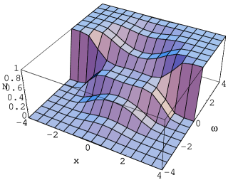
Figure 7: : $N(\omega,x)$ for $a=2\pi$ and $\gamma=0$.

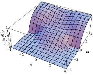
Figure 8: : $N(\omega,x)$ for $a=2\pi$ and $\gamma=1/2$.

5 Conclusions

We have undertaken the extension of a functional bosonization method, previously developed in the context of equilibrium field theory, to the case in which time-dependent perturbations are included. In particular, we have considered a model of fermions interacting through current-current interactions. In order to make contact with the description of 1D condensed matter systems those interactions are incorporated in a non-covariant way. In addition to this, by now standard (equilibrium) setting, we also included a term in the action -bilinear in fermion fields- which describes scattering through a time-dependent barrier. By using the CTP (Schwinger-Keldysh) approach to manage the time evolution of a field theory, we obtained the exact fermionic Green’s function for our out of equilibrium Thirring model (equation (3.28)). In the long-distance and long-time regime (the usual situation considered in the condensed matter context) we obtained a closed expression for the TED (equation (4)), which is a superposition of equilibrium TED’s centered at energies equal to integer multiples of the external half-frequency $\Omega/2$ . From this expression we readily obtained the time averaged TED $N(\omega,x)$ (equation (4.15)), in which only contributions corresponding to integer multiples of $\Omega$ survive, modulated by factors related to the spatial distribution of the impurity. Our results are consistent with the findings of the authors of ref. [11], who computed the temporal mean value of the TED for an arbitrary impurity geometry in a specific spatial point. In contrast to these authors, we included a temporal Heaviside function in the time dependent interaction. Although for this case we could not compute the TED for arbitrary scatterer geometries, by considering a rectangular barrier we were able to obtain explicit analytical results for the time-averaged TED, not only as function of energy but also in terms of the spatial coordinate.

This work could be continued in several directions. Firstly, it would be desirable to include the effect of finite temperature. Secondly, one could try to explore the short-time regime by building the TED using directly equation (3.28) for the Green’s function instead of the long-time approximation resulting through the simplified expression for $G_{C}^{\gamma}$ (equation (3.29)). This does not seem to be an easy task, but nevertheless we hope to follow this route in the close future.

References

-
[1]
E. Calzetta, B. L. Hu, Phys. Rev. D 35,
495, (1987); ibid. 37, 2878, (1988).
D. Boyanovsky, D. S. Lee, A. Singh, Phys. Rev. D 48, 800, (1993).
K. Rajagopal, F. Wilczek, Nucl. Phys. B 399, 395, (1993). - [2] F. Cooper, S. Habib, Y. Kluger, E. Mottola, J. P. Paz, Phys. Rev. D 50, 2848, (1994).
- [3] G. D. Mahan, Phys. Rep. 145, 251, (1987).
-
[4]
J. E. Moore, P. Sharma, C. Chamon, Phys. Rev. B
62, 7298, (2000).
A. Komnik, A.O. Gogolin, Phys. Rev. B. 66, 035407, (2002). -
[5]
J. Voit, Rep. on Prog. in Phys. 58, 977 (1995).
H. J. Schulz, G. Cuniberti and P. Pieri, cond-mat/9807366.
S. Rao and D. Sen, cond-mat/0005492.
C. M. Varma, Z. Nussinov and Wim van Saarloos, Phys. Rep. 351, 267, (2002), cond-mat/0103393.
R. Shankar, Rev. Mod. Phys. 66, 129 (1994). -
[6]
C.Naón, M.C.von.Reichenbach and M.L. Trobo,
Nucl. Phys. B 435[FS], 567, (1995);ibid. B 485 [FS], 665,(1997).
M.Manías, C.Naón , M.L.Trobo, Nucl. Phys. B 525 [FS], 721 (1998). -
[7]
J. Schwinger, J. Math. Phys. 2, 407, (1961).
L. V. Keldysh, Soviet Physics JETP 20, 1018, (1965).
K. Chou, Z. Su, B. Hao, L. Yu, Phys. Rep. 118, 1, (1985).
N. P. Landsman, Ch. G. van Weert, Phys. Rep. 145, 141, (1987).
A. Das, ”Finite Temperature Field Theory”, World Scientific Pub. Co. Ltd. (1997). -
[8]
S.Tomonaga, Prog. Theor. Phys. 5, 544, (1950).
J.Luttinger, J. Math. Phys. 4, 1154 (1963).
E.Lieb and D.Mattis, J. Math. Phys. 6, 304 (1965).
J.Solyom, Adv. Phys. 28, 209 (1979). - [9] D.Lee and Y. Chen, J. of Phys. A 21, 4155, (1988).
- [10] A. Iucci, C. Naón, hep-th/0311128, submitted for publication in Nucl. Phys. B.
- [11] A. Komnik, A.O. Gogolin, Phys. Rev. B 66, 125106, (2002).
- [12] D. E. Feldman, Y. Gefen, Phys. Rev. B 67, 115337, (2003).
- [13] K. Fujikawa, Phys. Rev. Lett. 42, 1195, (1979); Phys. Rev. D 21, 2848, (1980); Erratum-ibid. D22, 1499, (1980).
- [14] J. Voit, J. Phys.:Condens.Matter 5, 8305, (1993).
- [15] V. Meden, K. Schonhammer, Phys. Rev. B 46, 15753, 1992.
-
[16]
J. A. Stovneng, E. H. Hauge, J. Stat. Phys.
57, 841, (1989).
P. F. Bagwell, R. K. Lake, Phys. Reb. B 46, 15329, (1992). -
[17]
M. Bockrath, D. H. Cobden, J. Lu, A. G. Rinzler, R. E. Smalley, L. Balents,
P. L. Mc-Euen, Nature 397 598 (1999).
Z. Yao, H. W. J. Postma, L. Balents, C. Dekker, Nature 402 273 (1999). -
[18]
A. R. Goni et al., Phys. Rev. Lett. 67,
3298 (1991).
A. Yacoby, H. L. Stormer, N. S. Wingreen, L. N. Pfeiffer, K. W. Baldwin, K. W. West, Phys. Rev. Lett. 77, 4612, (1996).
O. M. Auslaender, A. Yacoby, R. de Picciotto, K. W. Baldwin, K. W. West, Science 295, 825, (2002).