Log-periodic behavior of finite size effects in field theories with RG limit cycles

Abstract

We compute the finite size effects in the ground state energy, equivalently the effective central charge $c_{\rm eff}$, based on S-matrix theories recently conjectured to describe a cyclic regime of the Kosterlitz-Thouless renormalization group flows. The effective central charge has periodic properties consistent with renormalization group predictions. Whereas $c_{\rm eff}$ for the massive case has a singularity in the very deep ultra-violet, we argue that the massless version is non-singular and periodic on all length scales.

I Introduction

Over the last few years a novel renormalization group (RG) scenario with limit-cycle behavior has been discovered in various models in a variety of physical contexts, including nuclear physics nuclear , quantum field theory BLflow ; LRS , quantum mechanics GW , superconductivity RDBCS , Bose-Einstein condensation Bose , and effective low energy QCD QCD . The subject of duality cascades in supersymmetric gauge theory Klebanov is also suggestive of limit-cycle behavior. The possibility of limit cycle behavior in the RG flow was considered as early as 1971 by Wilson Kwilson , however at the time no models with this behavior were known. The possibility of chaotic flows has also been recently considered GW ; morozov .

As is readily realized, models with cyclic RG flows have novel physical properties in comparison with theories with fixed points. For theories with bound states, the general signature of the cyclic RG is an infinite tower of bound states with energies related by discrete scaling relations nuclear ; GW ; RDBCS ; QCD , i.e. a self-similarity of the spectrum under a discrete scale transformation. This property was termed Russian doll scaling in RDBCS for obvious reasons. On the other hand, for continuous quantum field theories without bound states, the cyclic RG is manifested in the periodicity of the S-matrix as a function of energy LRS , as anticipated already by Wilson Kwilson .

The present article is a continuation of LRS . In the latter paper, an exact S-matrix for the cyclic regime of the Kosterlitz-Thouless flows was proposed for the first time. Using the S-matrices proposed there, here we investigate the finite-size effects, or equivalently the finite temperature effects, of the ground state energy $E(R)$ on a circle of circumference $R$ (temperature $1/R$). Conventionally one defines the effective central charge $c_{\rm eff}$ as $E(R)=-\pi c_{\rm eff}(R)/6R$. The quantity $c_{\rm eff}$ governs many physical properties, including the specific heat Cardy ; Affleck . It is known that for theories with fixed points, the quantity $c_{\rm eff}$ tracks the RG flow, namely, as a function of $R$ it smoothly interpolates between the ultra-violet (UV), $R=0$, and infra-red (IR), $R=\infty$, values of the Virasoro central charge of the fixed points ZamoTBA . For this reason $c_{\rm eff}$ is an interesting property to study for a model with an RG limit cycle, and this is the main subject of this paper. As we will show, it has a periodic structure as a function of $\log R$.

There is another c-function $c_{z}(L)$ which also tracks the RG flow between fixed points, this being the content of the celebrated c-theorem Zamoc ; Friedan , which is a statement of the irreversibility of the RG flow. Specifically the theorem states that $c_{z}(L)$ is a monotonically decreasing function of scale $L$ in the flow toward the IR. This by itself seems to rule out cyclic RG flows in unitary theories, since straightforward RG arguments show that $c_{z}(L)$ should be periodic in $\log L$. In fact the proof of the theorem constructs $c_{z}$ as a function of the couplings $g$, and the flow of $c_{z}$ is induced from the flow of $g$: $dc_{z}/d\log L=\beta_{g}\partial_{g}c_{z}(g)$, where $\beta_{g}$ is the $\beta$ function; thus if the couplings are periodic, so is $c_{z}$. Whereas $c_{\rm eff}(R)$ is related to a one-point function of the trace of the stress-energy tensor in a finite geometry (see below), $c_{z}(L)$ is related to a two-point function with fields separated by $L$ in infinite volume, and they are thus different. Nevertheless, for models with fixed points both $c_{\rm eff}(R)$ and $c_{z}(L)$ have essentially the same behavior, and we expect the same to be true for a theory with a cyclic RG. This leaves us with a paradox, since our theory is a perturbation of a unitary conformal field theory by a hermitian operator. This issue will not be dealt with any further in this work.

Let us now summarize our main results. In section II we outline the main features one expects for integrable, relativistic quantum field theories in 2d that have a cyclic RG, using only standard RG arguments in a model-independent way. There a clear distinction is made between massive and massless scattering theories. In section III we review the definition of the models and RG flows, extending the arguments to higher level $k$ current algebras. We point out two possible limiting theories, one massive, the other massless, depending on whether one has a UV or IR fixed point in the isotropic limit. In section IV we describe the proposed S-matrices. The massive S-matrix is the same as considered in LRS , whereas the massless one is new. Both these S-matrices are periodic in rapidity, which as explained in section II, is a clear signature of the cyclic RG. In section V we use thermodynamic Bethe ansatz techniques to study the finite size effects for the massive case. Though periodic structures consistent with the RG flows are found for $c_{\rm eff}$, in the deep UV it develops a singularity whose nature is explored in some detail. We derive an approximate analytic expression for $c_{\rm eff}$ in terms of Riemann’s zeta function, eq. (65) which is surprisingly simple and agrees very well with exact numerical results. The finite size-effects for the massless case are discussed in section VI; however at the present time the appropriate thermodynamic Bethe ansatz equations are unknown, and our analysis is thus incomplete. However on general grounds we argue that in the massless case $c_{\rm eff}$ should be an exactly periodic function of $\log R$ on all scales and has no singularities, and thus appears to be more consistent with the RG analysis.

II Physical Consequences of an RG limit cycle

In this section we describe some general properties that a model with an RG limit cycle should exhibit, as a way of anticipating our subsequent results.

Generally speaking, cyclic behavior in the RG flow can in principle exist at all scales, or can be approached asymptotically in the ultra-violet or infra-red, the latter being UV or IR limit-cycle behavior. Once the flow is in the cyclic regime, the couplings are periodic

$$g(l+\lambda)=g(l)$$ (1)

where $l=\log L$ and $L$ is the length scale. Above, the period $\lambda$ is fixed and model-dependent. In our model $\lambda$ is an RG invariant function of the two running couplings. As we will review in the next section, our models have a periodic RG on all scales rather than a limit cycle.

Consider first a theory of massive particles. In the deep IR, the particles appear infinitely heavy and decouple, leaving an empty theory which cannot support a low-energy limit cycle. Therefore, we expect that a massive theory can only support a UV limit cycle. A massless theory on the other hand can be non-trivial in the IR and thus support an IR limit cycle or a limit cycle on all scales. We will explore both possibilities subsequently.

II.1 RG equations for the S-matrix

It is well-known that the RG leads to certain scaling relations for the correlation functions (Callan-Symanzik equations). Since the S-matrix is obtained from momentum space correlation functions, it thus also obeys RG scaling relations.

Let $S$ denote the 2-particle to 2-particle S-matrix. For an integrable quantum field theory in 2 space-time dimensions, $S$ only depends on the kinematic variable $E_{\rm cm}^{2}=(P_{1}+P_{2})^{2}$ where $P_{1,2}$ are the energy-momentum vectors of the incoming particles. (For an integrable theory, the incoming and outgoing momenta are the same.) Standard RG arguments applied to the S-matrix lead to the scaling relation:

$$S(e^{-l}E_{\rm cm},g(l_{0}))=S(E_{\rm cm},g(l+l_{0})$$ (2)

(See e.g. ref. Ramond .) For a theory with a limit cycle, when $l=\lambda$ the above equation implies a periodicity in energy:

$$S(e^{-\lambda}E_{\rm cm},g)=S(E_{\rm cm},g)$$ (3)

Let us now specialize to 2d kinematics. First consider the massive case, where the energy momentum can be parameterized in terms of a rapidity $\beta$:

$$E=m\cosh\beta,~{}~{}~{}~{}~{}p=m\sinh\beta$$ (4)

where $m$ is the mass of the particles. The center of mass energy is

$$E_{\rm cm}^{2}=2m^{2}(1+\cosh\beta),~{}~{}~{}~{}~{}~{}~{}\beta=\beta_{1}-\beta_{2}~{}~{}~{}~{}~{}({\rm massive~{}case})$$ (5)

Suppose this theory has a UV limit cycle. At high energies $\beta$ is large and $E_{\rm cm}\approx me^{\beta/2}$. The relation eq. (3) then implies a periodicity in rapidity:

$$S(\beta-2\lambda)=S(\beta)$$ (6)

We turn now to the massless case. Here the massless dispersion relations $E=\pm p$ can be parameterized as:

$$E = {m\over 2}e^{\beta_{R}},~{}~{}~{}~{}~{}~{}p={m\over 2}e^{\beta_{R}},~{}~{}~{}~{}~{}~{}~{}~{}~{}~{}~{}{\rm for~{}right-movers}$$

$$E = {m\over 2}e^{-\beta_{L}},~{}~{}~{}~{}~{}p=-{m\over 2}e^{-\beta_{L}},~{}~{}~{}~{}~{}~{}~{}{\rm for~{}left-movers}$$ (7)

where now $m$ is an energy scale. The center of mass energy for a right-mover with rapidity $\beta_{R}$ scattering with a left-mover of rapidity $\beta_{L}$ is

$$E_{\rm cm}=me^{\beta/2},~{}~{}~{}~{}~{}~{}\beta=\beta_{R}-\beta_{L},~{}~{}~{}~{}~{}~{}({\rm massless~{}case})$$ (8)

If $S_{RL}(\beta)$ is the S-matrix for the scattering of right-movers with left-movers, then eq. (3) again implies a periodicity:

$$S_{RL}(\beta-2\lambda)=S_{RL}(\beta)$$ (9)

One sees then that the main difference between the massive and massive case is that in the massive case the periodicity in rapidity eq. (6) implies a periodicity in energy $E_{\rm cm}$ only for large $E_{\rm cm}$, whereas in the massless case it leads to a periodicity at all energy scales. Thus a massless theory with the periodicity eq. (9) is consistent with a cyclic RG flow on all scales, whereas the massive case at best can correspond to a theory with a limit cycle only in the deep UV.

II.2 RG equations for finite size effects

Let us consider the quantum field theory on a cylinder of finite circumference $R$ and length $L$ going to infinity. Viewing the finite circumference as the space the hamiltonian lives on, and the length $L$ as the time, the partition function behaves as

$$Z\sim e^{-LE(R)}$$ (10)

where $E(R)$ is the ground state energy of the hamiltonian at finite size $R$. This ground state scaling function contains a lot of information about the theory. From $E(R)$ one conventionally defines the effective central charge $c_{\rm eff}$:

$$E(R)=-{\pi\over 6}{c_{\rm eff}(R)\over R}$$ (11)

In theories with fixed points, $c_{\rm eff}(R)$ is equal to the Virasoro central charge $c$ at the fixed point, and smoothly interpolates between the ultra-violet and infra-red values of $c$. For this reason, it is very interesting to study $c_{\rm eff}$ in a theory with no fixed points but rather limit cycles.

In order to derive an RG scaling equation for $c_{\rm eff}$ we first relate it to a correlation function. Let $\langle T_{\mu}^{\mu}\rangle$ denote the one-point function of the trace of the stress-energy tensor on the cylinder. It is a function of the couplings $g$ and $R$, and is related to $c_{\rm eff}$ as follows ZamoTBA :

$$\langle T_{\mu}^{\mu}\rangle={2\pi\over R}{d\over dR}\left(RE(R)\right)=-{\pi^{2}\over 3R^{2}}{dc_{\rm eff}\over d\log R}$$ (12)

RG arguments applied to the one-point function give the scaling relation:

$$\langle T^{\mu}_{\mu}\rangle(e^{l}R,g(l_{0}))=e^{-2l}\langle T_{\mu}^{\mu}\rangle(R,g(l_{0}+l))$$ (13)

Taking $l$ to be equal to the period $\lambda$, one obtains:

$$c_{\rm eff}^{\prime}(e^{\lambda}R)=c_{\rm eff}^{\prime}(R),~{}~{}~{}~{}~{}c_{\rm eff}^{\prime}\equiv{dc_{\rm eff}(R)\over d\log R}$$ (14)

i.e. $c_{\rm eff}^{\prime}(R)$ is a periodic function of $\log R$ with period $\lambda$.

III The models and the cyclic RG flows

In this section we describe an action for our model and review the beta-function and RG flows. Consider a conformal field theory with $su(2)$ symmetry, described formally by the action $S_{\rm cft}$. The conformal symmetry promotes the $su(2)$ symmetry to decoupled left-right current algebra symmetry KZ , with left-moving (right-moving) currents $J^{a}(z)$ ($\overline{J}^{a}({\overline{z}})$), $a=+,-,3$ where $z=x+it,{\overline{z}}=x-it$ are euclidean light-cone space-time variables. The currents are normalized to satisfy the following operator product expansion:

$$J^{3}(z)J^{3}(0)\sim{k\over 2z^{2}},~{}~{}~{}~{}~{}J^{3}(z)J^{\pm}(0)\sim\pm{1\over z}J^{\pm}(0)~{}~{}~{}~{}~{}J^{+}(z)J^{-}(0)\sim{k\over 2z^{2}}+{1\over z}J^{3}(0)$$ (15)

where $k$ is the level, and similarly for the right-moving currents. The simplest realization of the current algebra is in terms of a pair of Dirac fermions, $J^{a}=\psi^{\dagger}\sigma^{a}\psi$, where $\sigma^{a}$ are Pauli matrices, and corresponds to a $k=1$ reducible representation with Virasoro central charge $c=2$. Our model is based on the irreducible level $k=1$ current algebra which can be represented in terms of the left-moving part of a free boson $\Phi=\phi(z)+\overline{\phi}({\overline{z}})$:

$$J^{3}={i\over\sqrt{2}}\partial_{z}\phi,~{}~{}~{}~{}~{}J^{\pm}={1\over\sqrt{2}}\exp\left({\pm i\sqrt{2}\phi}\right)$$ (16)

The action $S_{\rm cft}$ is then just the action for a free massless boson:

$$S_{\rm cft}={1\over 4\pi}\int d^{2}x~{}{1\over 2}(\partial_{\mu}\Phi)^{2}$$ (17)

and leads to $\langle\Phi(x)\Phi(0)\rangle=-\log|x|^{2}$. The above conformal field theory corresponds to Virasoro central charge $c=1$. (In the condensed matter context, the $c=1$ theory can be obtained from the $c=2$ theory by spin-charge separation.)

Our model is defined as an anisotropic left-right current-current perturbation of the conformal field theory:

$$S=S_{\rm cft}+\int{d^{2}x\over 2\pi}\left(4g_{\perp}(J^{+}\overline{J}^{-}+J^{-}\overline{J}^{+})-4g_{\parallel}J^{3}\overline{J}^{3}\right),$$ (18)

where $g_{\perp},g_{\parallel}$ are marginal couplings. The RG beta-functions determine how the couplings $g_{\parallel},g_{\perp}$ depend on the length scale $e^{l}$. These flows possess an RG invariant $Q$ satisfying $dQ/dl=0$. At one-loop, $Q=g_{\parallel}^{2}-g_{\perp}^{2}$. In a particular renormalization scheme, an all-orders beta-function has been conjectured GLM , and the higher order corrections to $Q$ are BLflow :

$$Q={g_{\parallel}^{2}-g_{\perp}^{2}\over(1+g_{\parallel})^{2}(1-g_{\perp}^{2})}.$$ (19)

The cyclic regime corresponds to $Q<0$. Let us parameterize:

$$Q\equiv-{h^{2}\over 16}$$ (20)

with $h>0$. The coupling $h$ is the main parameter of the theory. As shown in ref. LRS , it governs the period of the RG cycles:

$$g(\lambda+l)=g(l),~{}~{}~{}~{}~{}\lambda\equiv{2\pi\over h}$$ (21)

where $g=g_{\parallel,\perp}$. In each cycle $g_{\parallel}$ flows to $-\infty$ and jumps to $+\infty$. As described in BLflow one can view the coupling constant $-\arctan(4g_{\parallel}/h)$ as living on the universal cover of the circle. The physical quantities, such as the S-matrix and the finite size effects are all finite and as we will see reveal the RG cycles in a completely smooth manner. The above periodicity is not approached asymptotically, but is present on all scales; this will be an important criterion when we analyze the finite size effects.

The limit $h\to 0$ corresponds to being on one of either of the two separatrices $g_{\parallel}=\pm g_{\perp}$, which can be taken in the half-plane $g_{\perp}>0$ due to the symmetry $g_{\perp}\leftrightarrow-g_{\perp}$. These two $su(2)$ invariant theories are quite different. The theory with $g_{\parallel}=-g_{\perp}<0$ is a massive theory with UV fixed point at $g_{\parallel}=g_{\perp}=0$, and corresponds to the $su(2)$ invariant limit of the usual massive sine-Gordon theory with an empty IR fixed point. The theory with $g_{\parallel}=g_{\perp}>0$ on the other hand is a massless theory with a non-trivial IR fixed point at $g_{\parallel}=g_{\perp}=0$. In principle the UV behavior of the latter theory is not dictated by the action eq. (18); the action is rather an effective low-energy theory. However it is well understood that this flow can arise from the $O(3)$ sigma model at $\theta=\pi$, which is defined on all scales, in particular the UV. A massless S-matrix for this flow was given in ref. ZZflow . These observations lead us to consider two different S-matrix theories for the region $h\neq 0$. The first is the massive theory proposed in ref. LRS which when $h=0$ is the same as the sine-Gordon theory on the line $g_{\parallel}=-g_{\perp}<0$. The other theory, not considered in LRS , is a massless theory which corresponds to the $O(3)$ sigma model with $\theta=\pi$ in the limit $h=0$. As argued in section II, the massless theory is perhaps more consistent with the RG flow since it has the signature of a RG limit cycle on all length scales.

III.1 Higher k

In ref. GLM the beta-functions are given for arbitrary level $k$. The $k$-dependence is quite simple and can be scaled out of the RG flows by defining a new couplings $\widetilde{g}=kg$ and a rescaled RG time $\widetilde{l}=l/k$. In terms of $\widetilde{g}$ and $\widetilde{l}$ the flow equations are the same as for $k=1$. Thus the period in $l$ is $2\pi k/\widetilde{h}$, where $\widetilde{h}$ is defined by $\widetilde{Q}=-\widetilde{h}^{2}/16$, with $\widetilde{Q}$ the same as in eq. (19) with $g$ replaced by $\widetilde{g}$. However since the one-loop beta function does not depend on $k$, it is more sensible to normalize the RG invariant as :

$$Q={g_{\parallel}^{2}-g_{\perp}^{2}\over(1+kg_{\parallel})^{2}(1-k^{2}g_{\perp}^{2})}\equiv-{h^{2}\over 16}$$ (22)

since then $Q=g_{\parallel}^{2}-g_{\perp}^{2}+O(g^{3})$ and the leading one-loop contribution to $Q$ is the same for all $k$. One sees that $\widetilde{h}=kh$, and thus the period in $l$ is the same as for $k=1$: $\lambda=2\pi/h$ when $h$ is defined in the manner eq. (22).

In the next section we will propose an S-matrix for the higher $k$ theories.

IV The S matrices

IV.1 Massive case

In reference LRS it was conjectured that the cyclic regime of the KT flows described in the last section has a spectrum consisting of a massive soliton and anti-soliton with topological charge $\pm 1$. A factorisable S-matrix was proposed based on the ${\cal U}_{q}(\widehat{sl(2)})$ quantum affine symmetry of the underlying Hamiltonian where quantum parameter $q$ is related to the period $2\pi/h$ of the RG cycles by the equation

$$q=-e^{-\pi h/2}$$ (23)

This value of $q$ is rather unusual for a relativistic factorized S-matrix theory. The other previously known models with S-matrices related to a quantum affine symmetry all correspond to $q$ a pure phase, and are models with fixed points corresponding to free bosons or their quantum group reductions to minimal models when $q$ is a root of unity. S-matrices with a real $q$ however do appear in the study of the XXZ spin chain in the massive antiferromagnetic regime, where the solitons are understood as massive spinons. The relation of our model to the XXZ spin chain was discussed in LRS . There it was shown that in the low energy limit of small momentum, and as $h$ tends to zero, our S-matrix agrees with that of the spinons of the XXZ spin chain. However, in contrast to the spin chain, our dispersion relation is relativistic on all energy scales, as appropriate to the relativistic field theory of the last section, and this is the main difference between the models. As we will see, the interesting properties of the finite-size effects which are a consequence of the cyclic RG only appear in the ultraviolet limit for this massive case, and are thus unlikely to be properties of the spin-chain since the latter has an explicit lattice cut-off which leads to a non-relativistic dispersion relation.

We now describe in detail the S-matrix proposed in ref. LRS . As usual, we let $\beta$ parameterize the energy and momentum of the relativistic particles as in eq. (4), where $m$ is the mass of the soliton and anti-soliton. To describe their scattering amplitudes let us introduce the creation operators $A_{a}(\beta)$ for the solitons/antisolitons, where $a=\pm$ denotes the topological charge. The S-matrix may be viewed as encoding the exchange relation of these operators:

$$A_{a}(\beta_{1})A_{b}(\beta_{2})=S_{ab}^{cd}(\beta_{1}-\beta_{2})~{}A_{d}(\beta_{2})A_{c}(\beta_{1}).$$ (24)

The S-matrix can be presented in the following form:

$$S(\beta)=\left(\matrix{S_{++}^{++}&0&0&0\cr 0&S_{+-}^{+-}&S_{+-}^{-+}&0\cr 0&S_{-+}^{+-}&S_{-+}^{-+}&0\cr 0&0&0&S_{--}^{--}\cr}\right)={\rho(\beta)\over 2i}\left(\matrix{q\zeta-q^{-1}\zeta^{-1}&0&0&0\cr 0&\zeta-\zeta^{-1}&q-q^{-1}&0\cr 0&q-q^{-1}&\zeta-\zeta^{-1}&0\cr 0&0&0&q\zeta-q^{-1}\zeta^{-1}\cr}\right),$$ (25)

where $q$ is given in eq. (23), and

$$\zeta=e^{-i\beta h/2}.$$ (26)

($\beta=\beta_{1}-\beta_{2}$.) The overall scalar factor is:

$$\rho(q,\zeta)={2iq\over 1-q^{2}\zeta^{2}}\prod_{n=0}^{\infty}{(1-q^{4+4n}\zeta^{-2})(1-q^{2+4n}\zeta^{2})\over(1-q^{4+4n}\zeta^{2})(1-q^{2+4n}\zeta^{-2})}$$ (27)

This infinite product is convergent since $|q|<1$.

The above S-matrix satisfies the necessary constraints of crossing-symmetry, unitarity, real-analyticity and the Yang-Baxter equation. The factor $\rho$ can be understood as the minimal solution to crossing and unitarity when $q$ is real.

The arguments leading the above S-matrix are entirely independent of the RG analysis. Indeed the S-matrix depends on the couplings $g_{\perp},g_{\parallel}$ only through the RG invariant $h$. The physical mass $m$ also depends on the couplings, though in an unknown, non-perturbative fashion. It is therefore a non-trivial consistency check and confirmation of the cyclic RG if the S-matrix possesses the cyclicities discussed in section II. Indeed, it does possess the cyclicity eq. (6) with exactly the period $2\lambda$ predicted by the RG analysis based on the all-orders beta-function. This is easily verified since $\zeta(\beta+2\lambda)=\zeta(\beta)$. Recall that the period of the RG at one-loop is $h/\pi$ which is $\lambda/2$ LRS . Thus, that the all-orders beta-function correctly predicts the RG period is an indirect check of it.

S-matrices with real periodicities in the rapidity have previously been studied in Zelip ; Mussardo . Indeed, it was realized in Zelip that such a periodicity may imply an RG limit cycle; however at the time it was unknown what field theory the S-matrix described so it wasn’t possible to do an RG analysis. In these works, the S-matrix is expressed in terms of elliptic functions, whereas our S-matrix is trigonometric. For a single particle with diagonal scattering, crossing symmetry and unitarity lead to an imaginary $2\pi i$ periodicity, so that an additional real periodicity in $\beta$ naturally leads to the doubly periodic elliptic functions. Our S-matrix on the other hand is non-diagonal, and thus is not $2\pi i$ periodic, which explains why it can be expressed in terms of trigonometric functions.

One problem with the above massive S-matrix has already been alluded to. As discussed in section II, the above periodicity in rapidity implies an RG limit cycle only in the deep UV, which contradicts the flows described in section III which have limit cycles on all length scales. As we will see, other problems are encountered when we investigate $c_{\rm eff}$. We will argue that the massless S-matrix theory on the other hand doesn’t suffer from these problems.

For later purposes it is convenient to express the component $S^{++}_{++}$ as follows,

$$-i\log S^{++}_{++}(\beta)=\pi+{\beta h\over 2}+\sum_{n=1}^{\infty}{2\over n}{\sin(n\beta h)\over 1+e^{n\pi h}}$$ (28)

In the limit where $q\rightarrow-1$, i.e. $h\rightarrow 0$, it is easy to show that (28) becomes the $S^{++}_{++}$ entry of the sine-Gordon model at the $SU(2)$ invariant point ($SU(2)$ Thirring model):

$$-i\log S^{++}_{++}(\beta)=\pi+\int_{o}^{\infty}{dx\over x}\sin(\beta x){e^{-\pi x/2}\over\cosh(\pi x/2)}$$ (29)

IV.2 Massless case

An S-matrix description of theories with IR fixed points was given by Zamolodchikov and Zamolodchikov Zmassless ; ZZflow . An essential ingredient of their formulation are formal S-matrices for only left-movers or only right-movers, denoted $S_{LL}$ and $S_{RR}$. These S-matrices are formal S-matrices for a scale-invariant theory, and encode the information, such as the Virasoro central charge, of the infra-red fixed point. When left-right scattering $S_{RL}$ is non-trivial, the UV properties are affected. For the known models this collection of S-matrices corresponds to theories with non-trivial fixed points in both the UV and IR.

We now consider a massless S-matrix description of the limit cycle theory described in section III. Let us parameterize the massless energy momentum for left and right movers as in eq. (7). Requiring the two-particle S-matrices to correspond to the $O(3)$ sigma model at $\theta=\pi$ in the $su(2)$ invariant limit $h\to 0$ leads to the obvious proposal:

$$S_{RR}(\beta) = S_{h}(\beta),~{}~{}~{}~{}~{}\beta=\beta_{R1}-\beta_{R2}$$

$$S_{LL}(\beta) = S_{h}(\beta),~{}~{}~{}~{}~{}\beta=\beta_{L1}-\beta_{L2}$$ (30)

$$S_{RL}(\beta) = S_{h}(\beta),~{}~{}~{}~{}~{}\beta=\beta_{R1}-\beta_{L2}$$

where all the S-matrices $S_{h}$ on the right hand side are the same as in eq. (25).

The above S-matrix again has the periodicity anticipated in eq. (9). In this massless situation, this is a signature of cyclic RG on all length scales, entirely consistent with the RG flows.

IV.3 Higher $k$

In this subsection we propose S-matrices for the higher level $k$ models. In the limit where $h=0$, the model is the well-known isotropic current-current perturbation. In the massive case ($g_{\parallel}=-g_{\perp}<0$) the particles are known to have RSOS kink quantum numbers in addition to the spin $1/2$ $su(2)$ quantum numbers. The S-matrix factorizes $S^{(k)}=S_{su(2)}\otimes S_{RSOS}^{(k)}$ where $S_{su(2)}$ is the $su(2)$ invariant S-matrix of the $su(2)$ Thirring model and $S_{RSOS}^{(k)}$ is the k-th RSOS S-matrix which is a quantum group restriction of the usual sine-Gordon S-matrix (restricted sine-Gordon model) and occurs in the perturbations of the k-th $c<1$ minimal conformal series ABL . This factorization is a consequence of two commuting symmetries, the $su(2)$ and the (fractional) supersymmetry ABL .

Based on the above $h=0$ result, it is straightforward to propose an S-matrix for the k-th massive cyclic theory. When $h\neq 0$, the $su(2)$ symmetry becomes the ${\cal U}_{q}\left(\widehat{sl(2)}\right)$ symmetry with the same as above, the fractional supersymmetry is unaffected, and both symmetries continue to commute. The S-matrix is then:

$$S^{(k)}=S_{h}\otimes S^{(k)}_{RSOS}$$ (31)

where $S_{h}$ is the S-matrix described in eq. (25), and $S^{(k)}_{RSOS}$ is independent of $h$.

V Finite-size effects: massive case

V.1 Ground state scaling function

As discussed in section II, let us place our model on a cylinder of finite circumference $R$ and length $L$ going to infinity, and consider the ground state energy $E(R)$. In this section we consider only the massive case.

Given the S-matrix one can derive integral equations for $c_{\rm eff}$ by means of the thermodynamic Bethe ansatz (TBA) ZamoTBA . The derivation of the TBA equations for diagonal S-matrices given in ZamoTBA makes no reference to the usual Bethe ansatz for the eigenstates of a lattice regularization of the field theory, and relies only on knowledge of the S-matrix. Unfortunately for non-diagonal S-matrices the TBA normally leads to an infinite number of coupled integral equations for the pseudo-energies. However a dramatic simplification to a single integral equation has been found by Pearce and Klümper KlumperP , and Destri and de Vega DDV . In particular, Destri and de Vega (DdV) derived equations for the usual sine-Gordon theory based on a special scaling limit of the XXZ spin chain. Since as described above it is in principle possible to derive the TBA equations directly from the S-matrix alone, we can take the point of view that DdV indirectly have dealt with the mathematical complications of the non-diagonal nature of the scattering in the sine-Gordon theory. Since our S-matrix is essentially a sine-Gordon S-matrix with a real $q$ rather than a phase, we can thus obtain the TBA equations of our model from that of the sine-Gordon model equations by simply using our expression for the S-matrix.

V.2 The DdV equations

In the approach developed by DdV, the effective central charge has the following description in the usual sine-Gordon theory in the regime with only solitons in the spectrum:

$$c_{\rm eff}(R)={6mR\over\pi^{2}}\;{\Im{\it m}}\;\int_{-\infty}^{\infty}d\beta\;\sinh(\beta+i\alpha)\;\log(1+e^{iZ(\beta+i\alpha)})$$ (32)

where $m$ is the soliton mass and $Z$ is a solution of the non-linear integral equation:

$$Z(\beta)=mR\sinh\beta+2\;{\Im{\it m}}\int_{-\infty}^{\infty}d\beta^{\prime}\;G(\beta-\beta^{\prime}-i\alpha)\;\log(1+e^{iZ(\beta^{\prime}+i\alpha)})$$ (33)

The kernel $G(\beta)$ depends only on the soliton to soliton S-matrix element:

$$G(\beta)={1\over 2\pi i}{\partial\over\partial\beta}\log S^{++}_{++}(\beta)$$ (34)

Above, $0<\alpha<\pi/2$, is a regulator needed for convergence.

For the usual sine-Gordon model with $S^{++}_{++}$ given in ref. ZZ , $c_{\rm eff}(mR)$ is an uneventful function that smoothly interpolates between $c_{UV}=1$ in the ultra-violet ($R\to 0$) and $c_{IR}=0$ in the infra-red ($R\to\infty$). This reflects the existence of a $c=1$ UV fixed point, a free massless boson, and an empty IR fixed point. The fact that $c_{IR}=0$ is simply due to the fact that the theory is massive and in the deep IR these massive states decouple. This is in accordance with the rough picture that $c_{\rm eff}$ is in a sense a measure of the massless degrees of freedom: in the deep UV the massive particles are effectively massless and $c_{UV}=1$, whereas in the deep IR the massive particles decouple and $c_{IR}=0$. We have verified the above statements by solving the integral equation (33) numerically for the usual sine-Gordon model. The UV and IR limits of $c_{\rm eff}$ can also be computed analytically in terms of dilogarithms ZamoTBA ; DDV .

Because of the cyclic nature of the RG in our model, we expect a much more interesting behavior in the UV due to the non-existence of a fixed point. In the IR on the other hand, the usual argument given above applies since the theory is massive and one concludes $c_{IR}=0$.

For our model, the kernel has the simple expression:

$$G(\beta)={h\over 4\pi}\left[1+4\sum_{n=1}^{\infty}{\cos(n\beta h)\over 1+e^{n\pi h}}\right].$$ (35)

which follows from eqs. (34,28). The kernel has the following periodicity:

$$G\left(\beta+{2\pi\over h}\right)=G(\beta)$$ (36)

which is a clear indication of the cyclic RG, with the period exactly as predicted by the RG analysis reviewed in section III. It is this cyclicity of the kernel that is ultimately responsible for the non-trivial behavior of $c_{\rm eff}$ in the UV.

Let us first rewrite the DdV equations so that they resemble the more conventional expressions ZamoTBA , and also make them more suitable for numerical solution. Since $Z(\beta)$ is a real function when $\beta$ is real, let us define the pseudo-energies

$$\varepsilon(\beta)=-iZ(\beta+i\alpha),\qquad\varepsilon^{*}(\beta)=iZ(\beta-i\alpha),$$ (37)

Then eq. (33) can be written compactly as

$$\varepsilon=\varepsilon_{0}-G_{0}*L+G_{1}*L^{*},$$ (38)

where $*$ denotes a convolution

$$(f*g)(\beta)=\int_{-\infty}^{\infty}\;d\beta^{\prime}\;f(\beta-\beta^{\prime})\;g(\beta^{\prime}).$$ (39)

and we have defined:

$$\varepsilon_{0}(\beta) = -imR\sinh(\beta+i\alpha),$$ (40)

$$L(\beta) = \log(1+e^{-\varepsilon(\beta)}),$$ (41)

$$G_{0}(\beta) = G(\beta),\qquad G_{1}(\beta)\ =\ G(\beta+2i\alpha),$$ (42)

The expression for $c_{\rm eff}$ becomes

$$c_{\rm eff}(mR)={6\over\pi^{2}}\;\Re{\it e}\int_{-\infty}^{\infty}d\beta~{}\varepsilon_{0}(\beta)L(\beta)$$ (43)

We have solved the above equations numerically and verified that $c_{\rm eff}$ is independent of $\alpha$. A detailed presentation of our numerical results will be given below. For the further development of analytic results, the value $\alpha=\pi/2$ is preferred since then $\varepsilon_{0}=mR\cosh\beta$ is the standard pseudoenergy for a free theory, and when the kernel $G$ is zero, which occurs at the free fermion point of the usual sine-Gordon model, one has $\varepsilon=\varepsilon_{0}$ and the expression for $c_{\rm eff}$ is the standard free fermion one:

$$c_{\rm free}(mR)={6mR\over\pi^{2}}\int_{-\infty}^{\infty}d\beta\cosh\beta~{}\log(1+e^{-mR\cosh\beta})$$ (44)

In fact, in the usual sine-Gordon theory, $c_{\rm eff}$ is rather well approximated by $c_{\rm free}$ at all values of the coupling. Henceforth $\alpha$ will be set to $\pi/2$ in all analytic computations, and unless otherwise stated:

$$\varepsilon_{0}(\beta)=mR\cosh\beta.$$ (45)

It is convenient to define the function

$$\sigma(\beta)\equiv\varepsilon(\beta)-\varepsilon_{0}(\beta).$$ (46)

Since the kernels $G_{0,1}$ are periodic functions of $\beta$ with period $2\pi/h$, then so is $\sigma(\beta)$, and it can thus be expanded as a Fourier series:

$$\sigma(\beta)=\sum_{n=-\infty}^{\infty}\sigma_{n}~{}e^{inh\beta}$$ (47)

We can then proceed to rewrite the integral equations as non-linear algebraic equations for the various Fourier coefficients. First we expand the kernels:

$$G_{0}(\beta) = {h\over 2\pi}\sum_{n=-\infty}^{\infty}g_{0,n}e^{inh\beta},~{}~{}~{}~{}~{}g_{0,n}={1\over 1+e^{|n|\pi h}}$$ (48)

$$G_{1}(\beta) = {h\over 2\pi}\sum_{n=-\infty}^{\infty}g_{1,n}e^{inh\beta},~{}~{}~{}~{}~{}g_{1,n}=e^{-n\pi h}g_{0,n}.$$

Then the integral equation (38) can be written as

$$\sigma_{n}=-g_{0,n}L_{n}+g_{1,n}L_{-n},$$ (49)

where we have defined

$$L_{n}={h\over 2\pi}\int_{-\infty}^{\infty}d\beta~{}e^{-inh\beta}L(\beta),$$ (50)

with $L(\beta)$ as before but now viewed as a function of $\sigma$. In deriving eq. (49) we have used that $(L_{n})^{*}=L_{n}$, which is a consequence of $(L(\beta))^{*}=L(-\beta)$. From equation (49) one can derive the following relation:

$$\sigma_{n}=-{g_{1,n}\over g_{0,n}}\sigma_{-n}=-e^{-n\pi h}\sigma_{-n}.$$ (51)

which implies the absence of the zero mode, i.e. $\sigma_{0}=0$.

V.3 Exact Numerical results

The numerical work is simplified by splitting the various functions in the model, i.e. $f=\varepsilon,\sigma,L$, and the DdV equations into their real and imaginary parts (e.g. $f=f^{\prime}+if^{\prime\prime}$). Moreover the symmetry properties satisfied by these quantities further reduce the computational resources of the program. The kernel $G(\beta)$ in eq. (35) is an even function of $\beta$, and $Z(\beta)$ in eq. (33) is a real quantity. These facts imply that $Z(\beta)$ is an odd function of $\beta$, which in turn determines the parity properties of the remaining functions in the theory. Namely, the real parts, $f^{\prime}(\beta)$, are even, while the imaginary parts, $f^{\prime\prime}(\beta)$, are odd functions of $\beta$, and therefore $f(-\beta)=f^{*}(\beta)$.

The solution of the DdV equations has been found using two different methods: 1) recursive solution of the eq. (38) for the functions $\sigma^{\prime}(\beta)$ and $\sigma^{\prime\prime}(\beta)$; and 2) finding the roots of the non-linear system  (49) for the modes $\sigma_{n}$ subject to the constraint (51). The results obtained by these two methods are in full agreement.

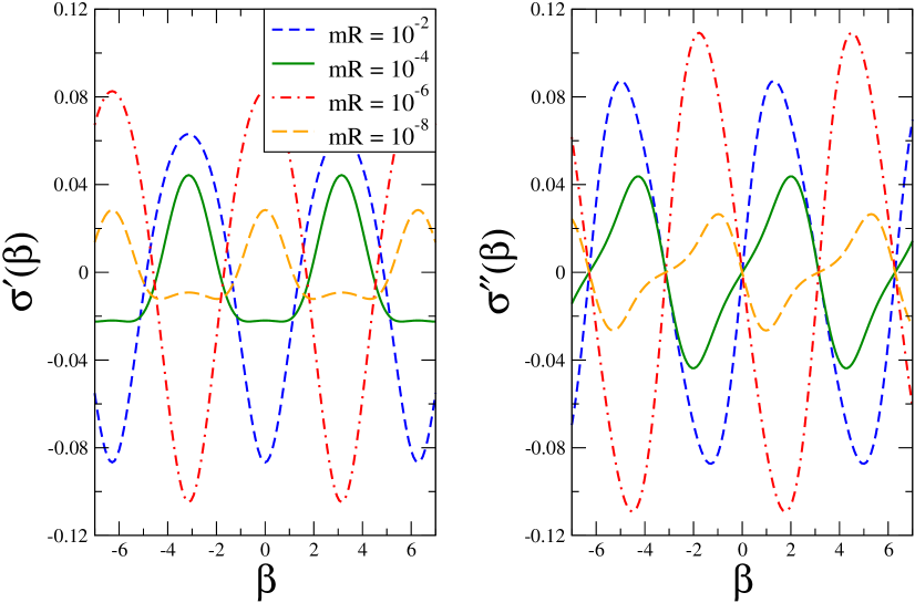
Figure 1: Solution of the eqs.(38) for $\sigma^{\prime}(\beta)$ and $\sigma^{\prime\prime}(\beta)$ for $h=1$, where $\sigma=\varepsilon-\varepsilon_{0}=\sigma^{\prime}+i\sigma^{\prime\prime}$.

In fig 1 we show the solution to eq. (38) in the case where $h=1$ and several values of $mR$ ranging from $mR=10^{-2}$ to $10^{-8}$. These results confirm that $\sigma^{\prime}$ is an even and periodic function of $\beta$ with period $2\pi/h$, while $\sigma^{\prime\prime}$ is an odd periodic function with the same period. We also observe that the amplitude of the oscillations is rather small, of order $10^{-2}$ in this case, which is a general feature except for special regions of $mR$ where the amplitudes are of order 1.

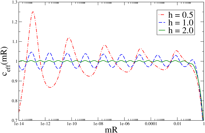
Figure 2: Exact numerical values of $c_{\rm eff}(mR)$ for $h=0.5,1,2$ in the range $mR=1-10^{-14}$.

Fig. 2 shows the values of $c_{\rm eff}(mR)$ corresponding to $h=0.5$, $1$, $2$ in the range $mR=1-10^{-14}$. In the IR region $c_{\rm eff}$ goes to $0$ exponentially fast and independently of the value of $h$, as expected for a massive model. As soon as $mR\lesssim 10^{-2}$, $c_{\rm eff}$ starts to oscillate around $c=1$ with a period $\pi/h$ in the scale, i.e.,

$$c(mR)\sim c(e^{\pi/h}mR)$$ (52)

Indeed, as seen in the figure, a complete cycle for the $h=0.5$ model contains two and four cycles of the $h=1$ and $h=2$ models respectively. Another feature of $c_{\rm eff}$ is that the amplitudes of the oscillations increase to-wards the UV, which is especially pronounced for $h=0.5$, and this is why eq. (52) is not an equality. The RG analysis performed in section III suggests a periodic $c_{\rm eff}(mR)$ function with period $2\pi/h$ in the scale, and this is twice what is observed numerically. This will be explained analytically in the next subsection.

V.4 Approximate analytic solution

In this subsection we derive an approximate analytic expression for $c_{\rm eff}$, explaining the properties observed numerically. Later we will show that it agrees remarkably well with the exact numerical solution to the full non-linear problem, and arguments for why this is so will be given.

We first make a linear approximation to the integral equation (49). Using

$$L(\beta)=L_{0}(\beta)-K(\beta)\sigma(\beta)+{\cal O}(\sigma^{2})$$ (53)

where

$$L_{0}(\beta)=\log(1+e^{-\varepsilon_{0}(\beta)}),~{}~{}~{}~{}~{}K(\beta)={1\over 1+e^{\varepsilon_{0}(\beta)}}$$ (54)

then to order $\sigma$:

$$L_{n}=L_{0,n}-\sum_{m}K_{n-m}\sigma_{m}$$ (55)

where $L_{0,n}$ and $K_{n}$ are Fourier transforms of $L_{0}$ and $K$:

$$L_{0,n}={h\over 2\pi}\int_{-\infty}^{\infty}d\beta\;e^{-inh\beta}L_{0}(\beta),~{}~{}~{}~{}~{}K_{n}={h\over 2\pi}\int_{-\infty}^{\infty}d\beta\;e^{-inh\beta}K(\beta)$$ (56)

Using eq. (55) in eq. (49) one finds the linear equations:

$$\sum_{m}A_{n,m}\sigma_{m}=B_{n}$$ (57)

where

$$A_{n,m} = \delta_{n,m}-g_{0,n}K_{n-m}+g_{1,n}K_{-n-m}$$ (58)

$$B_{n} = g_{1,n}L_{0,-n}-g_{0,n}L_{0,n}$$

In this approximation,

$$c_{\rm eff}(mR)\approx c_{\rm free}(mR)-{12\over\pi h}\sum_{n}\sigma_{n}K^{\prime}_{n}$$ (59)

where $K^{\prime}_{n}$ is the following Fourier transform:

$$K^{\prime}_{n}={h\over 2\pi}\int_{-\infty}^{\infty}d\beta\;e^{-inh\beta}K^{\prime}(\beta),~{}~{}~{}~{}~{}~{}K^{\prime}(\beta)\equiv\varepsilon_{0}(\beta)K(\beta)$$ (60)

All of the needed Fourier transforms $L_{0,n},K_{n},K^{\prime}_{n}$ are computed in appendix A. There the $mR$ dependence is expressed in terms of the logarithmic variable

$$s=\log\left(2\pi/mR\right)$$ (61)

In the deep UV where $R$ goes to $0$, $s$ is very large.

From the results in appendix A one finds in the UV limit of large $s$:

$$K_{0} \approx {h\over 2\pi}(s-\gamma-\log 2)$$ (62)

$$K_{n\neq 0} \approx -{h\over\pi\cosh(n\pi h/2)}{\Re{\it e}}\left(e^{inhs}\zeta_{1}(1-inh)\right)$$

where $\gamma$ is Euler’s constant and

$$\zeta_{1}(z)\equiv(1-2^{-z})\zeta(z)$$ (63)

with $\zeta$ Riemann’s zeta-function. Thus $K_{0}$ is large compared to $K_{n\neq 0}$ and this justifies the further approximation of keeping only the $K_{0}$ terms in eq. (57). ($K_{n\neq 0}$ is further suppressed by $e^{-n\pi h/2}$.) Using eq. (51), this essentially diagonalizes eq. (57) and one finds

$$\sigma_{n}\approx{B_{n}\over 1-2g_{0,n}K_{0}}$$ (64)

Using eq. (64) and the results in appendix A in eq. (59) one finds

$$c_{\rm eff}(mR)=c_{\rm free}(mR)+{24\over\pi}\sum_{n=1}^{\infty}{{\Im{\it m}}\left(e^{2insh}\zeta_{1}^{2}(-inh)\right)\over n(1+e^{n\pi h}-{h\over\pi}(s-\gamma-\log 2))}+{\cal O}(e^{-2s})$$ (65)

which is meant to be valid in the UV. The contribution $c_{\rm free}$ rapidly approaches $1$ in the UV.

A direct consequence of this equation, together with (61), is that the amplitudes of the oscillations of $c_{\rm eff}(mR)$ increases to-wards the UV because of the presence of a pole at the critical distance $R_{c,n}$

$$mR_{c,n}=\pi e^{-\gamma}\;\exp\left(-{\pi\over h}(1+e^{n\pi h})\right)$$ (66)

One sees that $c_{\rm eff}(mR)$ becomes singular at $R_{c,n}$ in this linear approximation. The double exponential in (66) implies that these scales are extremely small. For example the highest value of $R_{c,1}(h)$ is attained at $h=0.407$ where $mR_{c,1}=7.14\;10^{-16}$. Therefore at this scale we expect our approximation to break down. In the next subsection we shall study in more detail these critical points.

In fig. 3 we compare the result (65) with the exact numerical one for $h=0.8$ in the range $mR=1-10^{-20}$, observing a very good agreement over a wide range of distances. In this case the first critical distance is given by $mR_{c,1}=3.06\;10^{-23}$. Eq. (65) explains the oscillatory behavior of $c_{\rm eff}(mR)$ with a period $\pi/h$ in the scaling variable $s$. The lack of periodicity is due to the denominator of this expression which becomes more important as one approaches the critical points $R_{c,n}$.

The reason why the linear approximation is so good is that the higher order terms in the expansion of $L$ are in fact strongly suppressed in the deep UV (see Appendix B for details).

In fig. 4 we give a similar comparison for $h=0.4$ over a range that contains two critical distances $mR_{c,1}=7.09\;10^{-16}$ and $mR_{c,2}=5.33\;10^{-46}$.

Finally consider the $h\to 0$ limit, where the period $\lambda$ becomes infinitely large. The singularities at $R_{c,n}$ are pushed deeper and deeper to the UV and approach zero. One thus approaches a smooth flow between $c_{UV}=1$ and $c_{IR}=0$ as expected for the isotropic limit of the massive sine-Gordon theory.

A curious property of eq.(65) is that for the special value $h=h_{1}=2\pi/\log 2$ the linear contribution to $c_{\rm eff}$ vanishes as a consequence of the identity $\zeta_{1}(inh_{1})=0,\;\forall n$. Thus the value of $c_{\rm eff}$ is given simply by $c_{\rm free}$. The exact numerical solution also satisfies this result to order $10^{-16}$ which was our machine precision. For $h$ nearby $h_{1}$ the value of $c_{\rm eff}-c_{\rm free}$ is small but never zero. This fact is a consequence of the “absence” of the prime number 2 in Euler’s product formula for the zeta function $\zeta_{1}(z)$. For values of $h\neq h_{1}$ the corrections to $c_{\rm free}$ in eq. (65) are never zero since $\zeta(ih)$ does not vanish. The later quantity is related by the Riemann’s functional equation to $\zeta(1-ih)$ which does not vanish as well. The latter result was used by Hadamard and de la Vallée-Poussin to prove the prime number theorem zeta .

In summary, in the massive case the effective central charge $c_{\rm eff}$ exhibits nearly periodic structures over a large range of scales in the ultra-violet, with a period consistent with the RG predictions. However as one approaches the scales $R_{c,n}$ in the very deep ultraviolet, $c_{\rm eff}$ develops a singularity and the periodicity eq. (14) is violated. In the analytic approximation this singularity appears as a pole in $s$ in the equation (65). These features suggest that the massive theory is not entirely consistent with the RG flows, as alluded to in section IV.

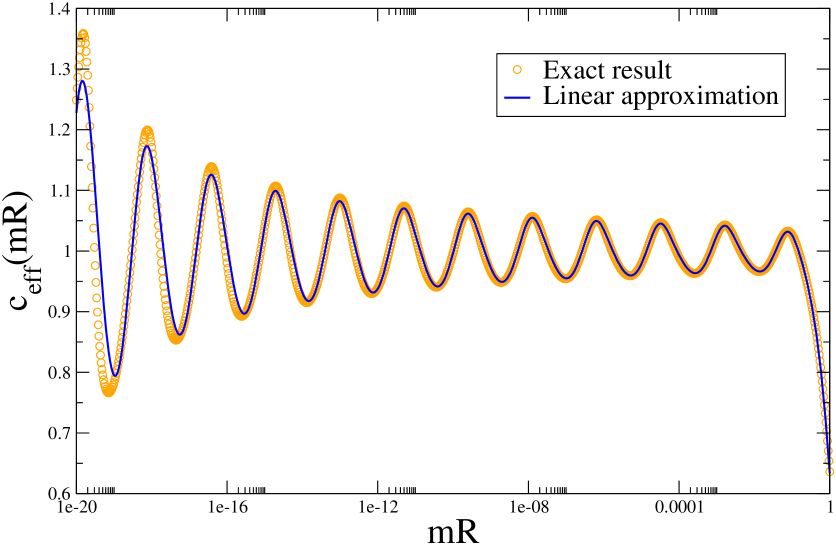
Figure 3: Comparison of $c_{\rm eff}(mR)$ computed with the analytic approximation eq.(65) and the exact numerical results for $h=0.8$

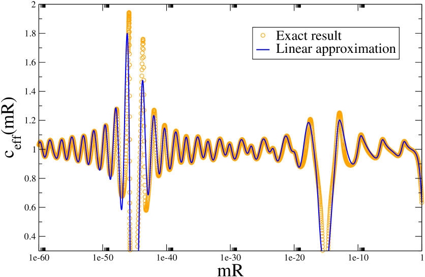
Figure 4: Comparison of $c_{\rm eff}(mR)$ computed with the analytic approximation eq.(65) and the exact numerical results for $h=0.4$

V.5 Coexistence regions

The approximate analytic solution of the DdV equations presented above explains the main features of the behavior of $c_{\rm eff}$, namely its periodicity and scale dependent amplitude. For most values of $mR$ the mode amplitudes $\sigma_{n}$ are rather small for all $n$, which explains the high accuracy of the analytic approximation. However at the critical values $R_{c,n}$ the $n^{\rm th}$ mode blows up and the analytic approximation is no longer valid, meanwhile the numerical solution still gives finite results.

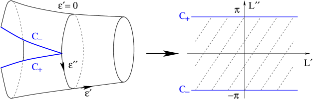
Figure 5: Conformal map $L(\varepsilon)=\log(1+e^{-\varepsilon})$ from the cylinder with a cut at $\varepsilon^{\prime}<0$ and $\varepsilon^{\prime\prime}=(2p+1)\pi$ into the strip $-\pi<{\Im{\it m}}L(\varepsilon)<\pi$.

Before we focus on this problem let us consider an important technical point regarding the definition of the logarithm $L(\beta)$ in (41). The imaginary part of $L(\beta)$ is the phase of $w(\beta)=1+e^{-\varepsilon(\beta)}$. For $-\infty<\beta<\infty$ the variable $w(\beta)$ describes a trajectory in the complex plane, which may pass through the cut of the logarithm, changing branches. As long as the modes $\sigma_{n}$ remain small enough this never happens. We have found that the solutions of the DdV eqs. belong to the principal branch of the logarithm, i.e. $-\pi<{\Im{\it m}}L(\beta)<\pi$. Under this condition $L(\varepsilon)$ becomes a conformal map from the cylinder with a cut at $\varepsilon^{\prime}<0$ and $\varepsilon^{\prime\prime}=(2p+1)\pi$, into the strip $-\pi<{\Im{\it m}}L(\varepsilon)<\pi$, as shown in fig. 5. The cut corresponding to $p=0$ translates into,

$$\varepsilon^{\prime} = \varepsilon^{\prime}_{0}+\sum_{n=1}^{\infty}\sigma^{\prime}_{n}\cos(nh\beta)\ <\ 0,\qquad\sigma^{\prime}_{n}=-\tanh(nh\alpha)\sigma^{\prime\prime}_{n},$$

$$\varepsilon^{\prime\prime} = \varepsilon^{\prime\prime}_{0}+\sum_{n=1}^{\infty}\sigma^{\prime\prime}_{n}\sin(nh\beta)\ =\ \pi,$$ (67)

and for $\alpha=\pi/2$ ($\varepsilon^{\prime\prime}_{0}=0$) these equations simplify. Since just one mode dominates the behavior of the system near the corresponding singularity, let us consider the single mode equations,

$$\varepsilon^{\prime} = mR\cosh\beta+\sigma^{\prime}_{n}\cos(nh\beta)\ <\ 0,\qquad\sigma^{\prime}_{n}=-\tanh(nh\pi/2)\sigma^{\prime\prime}_{n},$$

$$\varepsilon^{\prime\prime} = \sigma^{\prime\prime}_{n}\sin(nh\beta)\ =\ \pi,$$ (68)

which implies that $|\sigma^{\prime\prime}_{n}|<\pi$. Now we can solve the eqs. (49) for a single mode and search for the values of $R$ around $R_{c,n}$ satisfying $\sigma^{\prime\prime}_{n}=\pm\pi$. The results are shown in fig. 6.

This study of the logarithm solves the problem of the unbounded growth of $\sigma^{\prime\prime}_{n}$ and consequently $c_{\rm eff}(mR)$. In the IR there is a unique solution which evolves continuously to-wards the UV until it hits the cut, i.e. $|\sigma^{\prime\prime}_{n}|=\pi$, beyond which there is no solution. The boundary of the “IR phase” has a sawtooth shape which on average follows the analytic estimate (66) (see Fig. 6). For smaller values of $R<R_{c,1}$ one finds again a unique UV-solution which can be smoothly continued to-wards the IR until it hits the cut again. The boundary of this UV-solution has also a characteristic sawtooth shape as shown in Fig. 6. The IR and UV phases may coexist, meaning that there are two solutions for the same values of $mR$ and $h$. The regions with no IR/UV coexistence may contain isolated solutions non connected to the IR or UV regions, or they may not contain solutions at all. We have encountered both kinds of situations.The previous discussion concerns the truncation of the DdV equation to a single mode. Including all the modes yields an infinite number of coexistence regions, one for every mode, as shown already by the analytic approximation. The whole picture is as follows. Moving from the IR to-wards the UV, the first mode $\sigma^{\prime\prime}_{1}$ passes through its critical region and gets damped beyond it. Then, the second mode takes over and after a crossover region the period of $c_{\rm eff}$ doubles. This second mode also reaches its critical region and the process repeats itself with the third mode ( see fig. 4). Once more the analytic result fits amazingly well the exact numerical result including the proximity of the coexistence regions (for clarity we have truncated the analytic part very close to the pole).

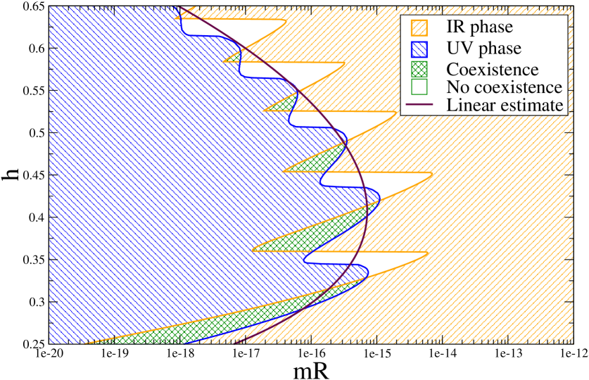
Figure 6: Coexistence of the IR and UV phases.

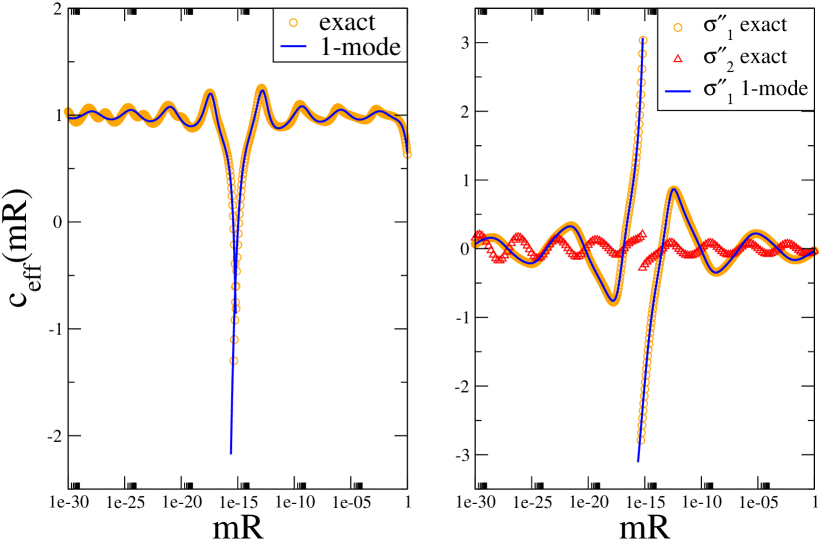
Figure 7: $c_{\rm eff}(mR)$ and the $\sigma^{\prime}_{1}$ and $\sigma^{\prime}_{2}$ in the region of the ”singularity” for $h=0.4$.

Finally, fig. 7 presents a comparison of the exact solution and the single mode approximation near the first singular region. At $h=0.4$ there is IR/UV coexistence as can be checked in fig. 6. Hence the IR and UV curves $c_{\rm eff}(mR)$ overlap around $mR\sim 10^{-15}$ (fig. 7a). Fig. 7b shows that the first mode of the exact solution, $\sigma^{\prime\prime}_{1}$, dominates over the second mode, $\sigma^{\prime\prime}_{2}$, which in the UV becomes more relevant. Notice also that $\sigma^{\prime\prime}_{1}$ is very well described by the single mode approximation.

VI Remarks on $c_{\rm eff}$ for the massless case

The structure of the TBA equations for massless theories has been understood in a number of models Zmassless ; fateev ; ZZflow . Unfortunately the massless DdV form of the equations are not known for the $O(3)$ sigma model at $\theta=\pi$, thus unlike the massive case, it is unknown what the $h=0$ limit of the TBA equations based on the S-matrices in eq. (30) should be. In spite of this, based on the known structure of massless TBA equations we can anticipate the general properties $c_{\rm eff}$ for theories based on massless S-matrices with limit cycles.

When the LR scattering is trivial, the S-matrices $S_{LL}$ and $S_{RR}$ describe a conformally invariant theory. Let us introduce pseudo-energies $\varepsilon_{L},\varepsilon_{R}$ separately for the left and right movers. As for other models, when the LR scattering is trivial the TBA equations are two decoupled integral equations for $\varepsilon^{L}$ and $\varepsilon^{R}$, each equation having the same form as a massive theory, the only difference being in the source terms $\varepsilon^{L}_{0},\varepsilon^{R}_{0}$ which now reflect the massless dispersion relations. Thus, when the left-right scattering is turned off, the TBA equations should just be two decoupled DdV equations of the kind described in section V. Turning on the left-right scattering $S_{LR}$ then couples the L,R integral equations.

Consider a toy model with only one particle with $S_{LL}=S_{RR}=1$ but a non-trivial $S_{LR}$, and define as usual the kernel as

$$G(\beta)={1\over 2\pi i}\partial_{\beta}\log S_{LR}$$ (69)

An example is the flow between the tricritical and critical Ising model Zmassless . Define the free pseudoenergies:

$$\varepsilon^{L}_{0}(\beta)={mR\over 2}e^{-\beta},~{}~{}~{}~{}~{}~{}\varepsilon^{R}_{0}(\beta)={mR\over 2}e^{\beta}$$ (70)

The structure of the TBA is the following:

$$\varepsilon^{L} = \varepsilon^{L}_{0}-G*L^{R}$$

$$\varepsilon^{R} = \varepsilon^{R}_{0}-G*L^{L}$$ (71)

where

$$L^{L,R}=\log\left(1+\exp({-\varepsilon^{L,R}})\right)$$ (72)

The effective central charge is:

$$c_{\rm eff}(mR)={6\over\pi^{2}}\Re{\it e}\int_{-\infty}^{\infty}d\beta~{}\left(\varepsilon^{R}_{0}L^{R}+\varepsilon^{L}_{0}L^{L}\right)$$ (73)

When the left-right pseudo-energies are decoupled, then by simple shifts of the rapidity one can show that $c_{\rm eff}(e^{l}R)=c_{\rm eff}(R)$ for any $l$ indicating a scale invariant conformal field theory with $c_{\rm eff}$ independent of $R$. When there is non-trivial LR scattering, which leads to the terms in eq. (71) which couple L and R, then $c_{\rm eff}$ becomes a function of $mR$.

Now consider an S-matrix that is periodic in rapidity, as for our model, such that $G(\beta+\lambda)=G(\beta)$, where as usual $\lambda$ is the period of the RG. An example of such an S-matrix for a single scalar particle was given in Mussardo . The due to the periodicity of the kernels $G$, $c_{\rm eff}$ is now invariant under a discrete scale transformation $e^{\lambda}$. To see this, one notes, using the periodicity of the kernels, that $\varepsilon_{L}(\beta-\lambda)$ and $\varepsilon_{R}(\beta+\lambda)$ satisfy the same integral equations as $\varepsilon_{L,R}$ but with $R$ replaced by $e^{\lambda}R$. Namely,

$$\varepsilon^{L}(\beta-\lambda,R)=\varepsilon^{L}(\beta,e^{\lambda}R),~{}~{}~{}~{}~{}\varepsilon^{R}(\beta+\lambda,R)=\varepsilon^{R}(\beta,e^{\lambda}R)$$ (74)

Using these equations in eq. (73) one can verify the periodicity of $c_{\rm eff}$:

$$c_{\rm eff}(e^{\lambda}R)=c_{\rm eff}(R)$$ (75)

The above exact periodicity of $c_{\rm eff}$ over all length scales is rather remarkable and entirely consistent with the RG argument that led to eq. (14). Also, it indicates that unlike the massive case, there is no scale dependence of the amplitudes of oscillation of $c_{\rm eff}$ and thus no singularities of the kind encountered in the last section.

VII Conclusions

We have analyzed the finite size effects, equivalently the finite temperature effects, in the ground state energy or effective central charge $c_{\rm eff}$ for the massive S-matrix theory proposed in LRS . The massive S-matrix was conjectured to describe the cyclic regime of the Kosterlitz-Thouless flows LRS . The S-matrices are periodic in the rapidities, with a period consistent with the RG analysis. This periodicity leads to novel finite size effects which also have periodic structures consistent with the cyclic RG. We obtained an approximate analytic expression for $c_{\rm eff}$ expressed in terms of Riemann’s zeta function eq. (65), which has log-periodic behavior and agrees remarkably well with the exact numerical solution.

For the massive case, there is a wide range of scales in the UV where $c_{\rm eff}$ oscillates. However in the very deep UV a singularity is encountered, and in some regions $c_{\rm eff}$ is not well defined (coexistence regions described in section V). This suggests the massive S-matrix theory needs an explicit UV cutoff in the very deep UV. For the massive case $c_{\rm eff}$ also lacks a periodicity on all scales as would be predicted by the RG.

For the massless case the TBA equations are unknown and we could not carry out the comparable analysis. However we argued on general grounds that the massless case should have some appealing properties. The $c_{\rm eff}$ should be exactly periodic on all scales, consistent with the RG. We hope to report on this in a future publication.

The log-periodic dependence of $c_{\rm eff}(mR)$ on $mR$ is reminiscent of the log-periodic fractal dimensions of self-similar fractals, such as the Cantor’s triadic set. Self-similarity amounts to discrete scale invariance, which in turn leads to log-periodic behavior in a wide variety of problems such as DLA (diffusion-limited-aggregation clusters), earthquakes, financial crashes, etc. sornette ; log ; tierz .

On a broader note, there appears to be a network of deeply interrelated concepts and techniques, namely RG limit cycles, discrete scale invariance, complex exponents, fractals, log-periodicity, quantum groups (with real $q$), zeta function regularizations, number theory, etc, whose full significance needs to be clarified.

Appendix A

In this appendix we compute the coefficients $F_{n}=\{L_{0,n},K_{n},K^{\prime}_{n}\}$ of the functions $F(\beta)=\{L_{0}(\beta),K(\beta),K^{\prime}(\beta)\}$ needed in section V-D. They are given by the formula

$$F_{n}={h\over 2\pi}\widehat{F}(nh)$$ (76)

where $\widehat{F}(t)$ is the Fourier transform of $F$:

$$\widehat{F}(t)\equiv\int_{-\infty}^{\infty}d\beta\;F(\beta)\;e^{-it\beta}$$ (77)

VII.1 Fourier transform of $K(\beta)$

The function $K(\beta)$ is given by

$$K(\beta)={1\over 1+\exp(r\cosh(\beta))}$$ (78)

where $r=mR$ is the scaling variable. Since $K(\beta)$ is an even function we can write its Fourier transform (77) as

$$\widehat{K}(t)\equiv\int_{-\infty}^{\infty}d\beta\;{e^{it\beta}\over 1+\exp(r\cosh(\beta))}$$ (79)

For $t>0$ one can evaluate (79) as the sum of the residues of the poles of $K(\beta)$ in the upper half plane ${\Im{\it m}}\beta>0$. These poles are the zeros of the denominator of $K(\beta)$ and are given by

$$\beta^{\pm}_{p,p^{\prime}} = \pm\theta_{p}+i{\pi\over 2}(1+2p^{\prime}),\quad p,p^{\prime}\geq 0$$ (80)

$$\theta_{p} = \sinh^{-1}\left({\pi(1+2p)\over r}\right)$$

The residue formula yields

$$\widehat{K}(t)=-{2\pi\over r\cosh(\pi t/2)}\;\sum_{p=0}^{\infty}{\cos(t\theta_{p})\over\cosh\theta_{p}}$$ (81)

For $t>0$ and real this series diverges. We shall regularize it using the Riemann zeta function $\zeta(z)$. For simplicity let us consider the UV limit $r\rightarrow 0$ where $\theta_{p}$ has the expansion,

$$\theta_{p}=s+\log(1+2p)+{e^{-2s}\over(1+2p)^{2}}+O(e^{-4s})$$ (82)

where $s=\log(2\pi/r)$. The series (81) becomes

$$\widehat{K}(t)=-{1\over\cosh(\pi t/2)}\;\sum_{p=0}^{\infty}\left[e^{its}\left({1\over(1+2p)^{1-it}}-e^{-2s}{(2-it)\over(1+2p)^{3-it}}\right)+(t\rightarrow-t)\right]+O(e^{-4s})$$ (83)

The sums in $p$ can be done using the Riemann zeta function $\zeta(z)$

$$\zeta(z)=\sum_{n=1}^{\infty}\;{1\over n^{z}}$$ (84)

together with the relation:

$$\sum_{p=0}^{\infty}{1\over(1+2p)^{z}}=(1-2^{-z})\;\zeta(z)\equiv\zeta_{1}(z)$$ (85)

This gives

$$\widehat{K}(t)=-{1\over\cosh(\pi t/2)}\;\left[e^{its}\left[\zeta_{1}(1-it)-e^{-2s}(2-it)\zeta_{1}(3-it)\right]+(t\rightarrow-t)\right]+O(e^{-4s})$$ (86)

Strictly speaking eqs.(84) and (85) are only defined when ${\Re{\it e}}\;z>1$. However the Riemann zeta function is defined in the entire complex plane except at $z=1$ where it has a pole. Our use of $\zeta(z)$ is completely analogous to other situations in quantum field theory where it serves to regularize formal expressions.

Equation (76) gives the Fourier coefficients

$$K_{n}={h\over 2\pi}\;\widehat{K}(nh)$$ (87)

In the UV limit the terms proportional to $e^{-2ps}\;\;(p=1,2,\dots)$ vanish very rapidly and one is left with the oscillating terms that depend on $\zeta_{1}(1\pm it)$. The value $K_{0}$ is special since $\zeta(z)$ behaves near $z=1$ as

$$\zeta(z)\sim{1\over z-1}+\gamma$$ (88)

where $\gamma$ is the Euler’s constant. Using this equation the value of $K_{0}$ is given by

$$K_{0}={h\over 2\pi}\left(s-\gamma-\log 2+{7\zeta(3)\over 2}e^{-2s}\right)+O(e^{-4s})$$ (89)

The linear dependence of $K_{0}$ with $s$ in the UV limit can be easily understood using the “kink method” proposed by Zamolodchikov to study the UV limit of usual massive models ZamoTBA . From eq.(77,76) we have

$$K_{0}={h\over 2\pi}\int_{-\infty}^{\infty}d\beta\;{1\over 1+\exp({r\cosh\beta})}$$ (90)

which in the limit $r\ll 1$ can be approximated as

$$K_{0}={h\over\pi}\int_{0}^{\infty}d\beta\;{1\over 1+\exp(e^{\beta-s^{\prime}})}$$ (91)

where $s^{\prime}=\log(2/r)\gg 1$. From this expression it is clear that the integrand remains close to $1/2$ for $0<\beta\lesssim s^{\prime}$ and that it vanishes exponentially for $\beta\gg s^{\prime}$. Hence $K_{0}\sim hs^{\prime}/(2\pi)$ which agrees with eq.(89) up to constant terms since $s^{\prime}=s-\log\pi$.

VII.2 Fourier transform of $K^{\prime}$

The function $K^{\prime}(\beta)$ is defined as

$$K^{\prime}(\beta)=\varepsilon_{0}(\beta)K(\beta)$$ (92)

Following the same steps as in the previous subsection we find the Fourier transform,

$$\widehat{K^{\prime}}(t)={2\pi\over\sinh(\pi t/2)}\;\sum_{p=0}^{\infty}\tanh(\theta_{p})\sin(t\theta_{p})$$ (93)

In the UV limit this can be approximated as

$$\widehat{K^{\prime}}(t)=-{i\pi\over\sinh(\pi t/2)}\;\left[e^{its}\left[\zeta_{1}(-it)-e^{-2s}(2-it)\zeta_{1}(2-it)\right]-(t\rightarrow-t)\right]+O(e^{-4s})$$ (94)

where we have included explicitly the term of order $e^{-2s}$ as in eq.(86). The value of this function at $t=0$ is given by

$$\widehat{K^{\prime}}(0)=-4\zeta(0)\,\log 2=2\log 2$$ (95)

where we have used that $\zeta(0)=-1/2$.

Using the kink method one can see that this result is equivalent to the following integral

$$2\log 2={1\over 2}\int_{-\infty}^{\infty}d\beta~{}{e^{\beta}\over 1+\exp(e^{\beta}/4)}$$ (96)

which can be checked numerically to any precision.

VII.3 Fourier transform of $L_{0}(\beta)$

The function $L_{0}(\beta)$ is defined as

$$L_{0}(\beta)=\log(1+e^{-r\cosh\beta})$$ (97)

To compute its Fourier transform we note that

$$-r{d\over dr}L_{0}(\beta)={d\over ds}L_{0}(\beta)=K^{\prime}(\beta)$$ (98)

Hence the Fourier transform of $L_{0}(\beta)$ can be obtained integrating eq.(98) in $s$, obtaining:

$$\widehat{L_{0}}(t)=-{\pi\over\sinh(\pi t/2)}\;\left[e^{its}\left({1\over t}\zeta_{1}(-it)+ie^{-2s}\zeta_{1}(2-it)\right)+e^{-its}\left({1\over t}\zeta_{1}(it)-ie^{-2s}\zeta_{1}(2+it)\right)\right]$$ (99)

The integration constant is zero as we shall next show. Let us consider the value of $\widehat{L_{0}}(0)$:

$$\widehat{L_{0}}(0)=2\,s\log 2-\log 2\,\log(2\pi^{2})$$ (100)

where we have used that $\zeta^{\prime}(0)=-{1\over 2}\log(2\pi).$ Notice that the leading term in $s$ coincides with the value of $\widehat{K^{\prime}}(0)$ given in eq.(95), but there is a constant term that appears in the limit $t\rightarrow 0$ in (99). Using the kink method eq. (99) amounts to,

$$\lim_{r\rightarrow 0}\left[2\int_{0}^{\infty}d\beta\log(1+\exp(-r\cosh\beta))-2s\,\log 2\right]=-\log 2\,\log(2\pi^{2}),\quad\quad s=\log(2\pi/r)$$ (101)

which we checked numerically. This shows that the integration constant relating $\widehat{K^{\prime}}(t)$ and $\widehat{L_{0}}(t)$ vanishes.

Appendix B

In this appendix we justify the analytic approximation made in section V-D of the non linear eq.(49).

The full expansion of the function $L(\beta)$ is given by

$$L(\beta)=L_{0}(\beta)-\sum_{a=1}^{\infty}{\sigma^{a}\over a!}\;K^{(a-1)}(\beta)$$ (102)

where

$$K^{(a)}(\beta)={d^{a}K\over d\varepsilon_{0}^{a}},\qquad K^{(0)}\equiv K={1\over 1+e^{\varepsilon_{0}}}$$ (103)

Using eq.(102), the expansion of eq.(49) to all orders in $\sigma$ becomes,

$$\sum_{m}A_{n,m}\sigma_{m}=B_{n}+\sum_{a=2}^{\infty}{1\over a!}\sum_{m_{1},\cdots,m_{a}}C^{a}_{n,\;\sum m_{i}}\;\;\sigma_{m_{1}}\cdots\sigma_{m_{a}}$$ (104)

where $A_{n,m}$ and $B_{n}$ were defined in eq.(58) and

$$C^{a}_{n,m} = g_{0,n}K^{(a-1)}_{n-m}-g_{1,n}K^{(a-1)}_{-n-m},$$ (105)

$$K^{(a)}_{n} = {h\over 2\pi}\int_{-\infty}^{\infty}d\beta\;e^{-inh\beta}K^{(a)}(\beta)={h\over 2\pi}\widehat{K}^{(a)}(nh)$$

The analytic approximation of section V-D consists in i) eliminating the terms O($\sigma^{n}$), with ${n\geq 2}$, in eq.(104) yielding eq.(58), and ii) considering only the coefficient $K_{0}$ which depends linearly on the scale $s$ (recall eq.(62)). The latter asumption is justified if the $\sigma_{n}$’s are small enough. As for the first assumption we shall show below that the terms in eq.(104) containing high powers in $\sigma_{n}$ do not depend linearly on the scale $s$, and can thus be neglected in the UV.

The Fourier transform of $K^{(a)}$ can be found by the techniques of appendix A and it reads,

$$\widehat{K}^{(a)}(t)=-\left({-i\over\pi}\right)^{a}\sum_{\nu=\pm 1}e^{it\nu s}\;{\Gamma(a+1-it\nu)\over\Gamma(1-it\nu)}\;\zeta_{1}(a+1-it\nu)\times\left\{\begin{array}[]{ll}1/\cosh(\pi t/2),&a=0,2,\dots\\ \nu/\sinh(\pi t/2),&a=1,3,\dots\end{array}\right.$$ (106)

The case $a=0$ agrees with eq. (86). Let us focus on the cases where $a\geq 1$. Only for $t=0$ one may get a linear dependence on $s$, namely

$$\widehat{K}^{(a)}(0)=a!\;\zeta_{1}(a+1)\times\left\{\begin{array}[]{ll}-2\left({i\over\pi}\right)^{a},&a=2,4,\dots\\ 4\left({i\over\pi}\right)^{a+1}s,&a=1,3,\dots\\ \end{array}\right.$$ (107)

Returning to eq.(104), the only terms that may contribute linearly in $s$, are

$$\sum_{a\geq 2,\;{\rm even}}s\;{2h\;\zeta_{1}(a)i^{a}\over a\;\pi^{a+1}}\left(g_{0,n}\sum_{{m_{1}},\dots,{m_{a}}}\delta_{n,m_{1}+\dots+m_{a}}\;\sigma_{m_{1}}\dots\sigma_{m_{a}}-g_{1,n}\sum_{{m_{1}},\dots,{m_{a}}}\delta_{-n,m_{1}+\dots+m_{a}}\;\sigma_{m_{1}}\dots\sigma_{m_{a}}\right)$$ (108)

Using eq.(51) one can show that

$$\sum_{{m_{1}},\dots,{m_{a}}}\delta_{n,m_{1}+\dots+m_{a}}\;\sigma_{m_{1}}\dots\sigma_{m_{a}}=(-1)^{a}e^{-n\pi h}\sum_{{m_{1}},\dots,{m_{a}}}\delta_{-n,m_{1}+\dots+m_{a}}\;\sigma_{m_{1}}\dots\sigma_{m_{a}}$$ (109)

which together with eq.(48), namely $g_{1,n}=e^{-n\pi h}g_{0,n}$, implies the vanishing of (108). In summary, all the linear dependence in $s$ of the eq.(104) comes from the coefficient $B_{n}$.

References

- (1) P. F. Bedaque, H.-W. Hammer, and U. van Kolck, “Renormalization of the Three-Body System with Short-Range Interactions”, Phys. Rev. Lett. 82 (1999) 463, nucl-th/9809025.
- (2) D. Bernard and A. LeClair, “Strong-weak coupling duality in anisotropic current interactions”, Phys.Lett. B512 (2001) 78; hep-th/0103096.
- (3) A. LeClair, J.M. Román and G. Sierra, “Russian Doll Renormalization Group and Kosterlitz-Thouless Flows”, Nucl. Phys. B to appear; hep-th/0301042.
- (4) S. D. Glazek and K. G. Wilson, “Limit cycles in quantum theories”, hep-th/0203088; “Universality, marginal operators, and limit cycles,” cond-mat/0303297.
- (5) A. LeClair, J.M. Román and G. Sierra, “Russian Doll Renormalization Group and Superconductivity”, Rapid Communications of Phys. Rev. B to appear; cond-mat/0211338.
- (6) E. Braaten, H.-W. Hammer, and M. Kusunoki, “Efimov States in a Bose-Einstein Condensate near a Feshbach Resonance”, Phys.Rev.Lett. 90 (2003) 170402, cond-mat/0206232.
- (7) E. Braaten and H.-W. Hammer, “An Infrared Renormalization Group Limit Cycle in QCD”, Phys.Rev.Lett. 91 (2003) 102002, nucl-th/0303038.
- (8) I.R. Klebanov and M. J. Strassler, “Supergravity and a Confining Gauge Theory: Duality Cascades and SB-Resolution of Naked Singularities”, JHEP 0008 (2000) 052, hep-th/0007191.
- (9) K. G. Wilson, “Renormalization Group and Strong Interactions”, Phys. Rev. D3 (1971) 1818.
- (10) A. Morozov and A. J. Niemi, “Can Renormalization Group Flow End in a Big Mess?”, hep-th/0304178.
- (11) J. Cardy, “Conformal Invariance and Universality in Finite-size Scaling”, J. Phys. A17 (1984) 385.
- (12) I. Affleck, “Universal term in the Free Energy at a Critical Point and the Conformal Anomaly”, Phys. Rev. Lett. 56 (1986) 746.
- (13) A.B. Zamolodchikov, “Thermodynamic Bethe Ansatz in Relativistic Models. Scaling 3-state Potts and Lee-Yang models”. Nucl.Phys.B342, 695 (1990).
- (14) A. B. Zamolodchikov, “Irreversibility of the flux of the renormalization group in a 2D field theory”, JETP Lett 43, 731 (1986).
- (15) A. Cappelli, D. Friedan and J. Latorre, “c-theorem and spectral representation”, Nucl.Phys. B352 (1991) 616.
- (16) M. Peskin and D. Schroeder, “An Introduction to Quantum Field Theory”, Addison-Wesley, 1995.
- (17) V. G. Knizhnik and A.B. Zamolodchikov, “Current algebras and the Wess-Zumino model”, Nucl. Phys. B247, 83 (1984).
- (18) B. Gerganov, A. LeClair and M. Moriconi, “On the Beta Function for Anisotropic Current Interactions in 2D”, Phys. Rev. Lett. 86 (2001) 4753; hep-th/0011189.
- (19) V. A. Fateev and Al. B. Zamolodchikov, “Integrable perturbations of Z(N) parafermion models and O(3) sigma model”, Phys.Lett. B271 (1991) 91.
- (20) A. B. Zamolodchikov and Al. B. Zamolodchikov, “Massless factorized scattering and sigma models with topological terms”, Nucl.Phys.B379 (1992) 602.
- (21) C. Ahn, D. Bernard and A. LeClair, Nucl. Phys. B346 (1990) 409; D. Bernard and A. LeClair, Phys. Lett. B247 (1990) 309.
- (22) A. B. Zamolodchikov, Commun. Math. Phys. 69 (1979) 253.
- (23) G. Mussardo and S. Penati, “A quantum field theory with infinite resonance states”, Nucl. Phys. B567 (2000) 454, hep-th/9907039.
- (24) P. A. Pearce and A. Klümper, “Finite-size corrections and scaling dimensions of solvable lattice models: An analytic method”, Phys. Rev. Lett. 66, 974 (1991).
- (25) C. Destri and H.J. de Vega, “Unified Approach to Thermodynamic Bethe Ansatz and Finite Size Corrections for Lattice Models and Field Theories”, Nucl.Phys. B438 (1995) 413; hep-th/9407117.
- (26) A. B. Zamolodchikov and Al. B. Zamolodchikov, “Factorized S-matrices in Two Dimensions as the Exact Solutions of Certain Relativistic Quantum Field Theory Models”, Annals of Phys. 120, 253 (1979).
- (27) Al. B. Zamolodchikov, “From tricritical Ising to critical Ising by Thermodynamic Bethe anstaz”, Nucl.Phys.B358 (1991) 524.
- (28) H.M. Edwards, “Riemann’s zeta function”, Eds. S. Eilenberg and H. Bass, Academic Press, INC. San Diego.
- (29) D. Sornette, “Discrete scale invariance and complex dimensions”, Phys. Rep. 297, 239 (1998); cond-mat/9707012.
- (30) S. Gluzman and D. Sornette, “Log-periodic route to fractal functions”, Phys. Rev. E 65, 036142 (2002); cond-mat/0106316.
- (31) M. Tierz, “Spectral behavior of models with a quantum group symmetry”, hep-th/0308121.