Branes, Strings, and Odd
Quantum Nambu Brackets

Abstract

The dynamics of topological open branes is controlled by Nambu Brackets. Thus, they might be quantized through the consistent quantization of the underlying Nambu brackets, including odd ones: these are reachable systematically from even brackets, whose more tractable properties have been detailed before.

1 Classical Nambu Dynamics

The classical motion of topological open membranes is controlled by Nambu Brackets, the multilinear generalization of Poisson Brackets.[1] We have addressed even branes before, in Refs sphere,CQNB,talks, but not odd ones, treated here, essentialy by reduction to even ones, in a parallel solution of the problem.

Consider the “vortex string” 2-form action,[5, 6, 7, 8, 4]

$$S=\int\Bigl{(}z^{1}~{}dz^{2}\wedge dz^{3}-H~{}dG\wedge dt\Bigr{)}~{},$$ (1)

originating in an exact 3-form,

$$d\omega_{2}=dz^{1}\wedge dz^{2}\wedge dz^{3}-dH\wedge dG\wedge dt~{},$$ (2)

(in analogy to the Hamilton-Poincaré symplectic 2-form, $d\omega_{1}=dx\wedge dp_{x}+dH\wedge dt$). The 3-integral of this form on an open 3-surface yields the above 2-form action evaluated on the 2-boundary of that surface, i.e., a Cartan integral invariant, analogous to the $(1+1)$-dimensional $\sigma$-model WZW topological interaction terms or Chern-Simons actions.

More explicitly, in world-sheet coordinates $t,\sigma$, the action reads

$$S=\int dtd\sigma~{}\left({\epsilon^{ijk}\over 3}z^{i}\partial_{t}z^{j}\partial_{\sigma}z^{k}+H\partial_{\sigma}G\right)~{}.$$ (3)

For such systems, Dirac quantization procedures have been outlined in, e.g., Refs rasetti,mukunda,Bayen; but they are cumbersome to complete, insofar as they rely on Kontsevich’s generalization[12] of Moyal Brackets to nonflat Poisson manifolds, if they are to lead to explicit consistent results, and will not be considered here. Instead, we utilize the linkage of the above action (and actions of this broad type) to Nambu Brackets (NB).

The classical variational equations of motion of the action resulting from $\delta z^{i}$ are

$$0=(\epsilon^{ijk}\partial_{t}z^{j}+\partial_{i}H\partial_{k}G-\partial_{k}H\partial_{i}G)~{}\partial_{\sigma}z^{k}.$$ (4)

Motion along the string (along $\partial_{\sigma}z^{i}$) may be gauge-fixed by virtue of $\sigma$ reparameterization invariance,[7] so that this reduces to

$$\dot{z}^{i}=\epsilon^{ijk}\partial_{j}H\partial_{k}G~{},$$ (5)

and these amount to Nambu’s dynamical equations,[1]

$$\dot{z}^{i}={\partial(z^{i},H,G)\over\partial(z^{1},z^{2},z^{3})}\equiv\{z^{i},H,G\}.$$ (6)

In this context, this Jacobian determinant (volume element), defines the Nambu 3-bracket, which generalizes and supplants the Poisson Bracket, and is likewise linear and antisymmetric in its arguments —here, with two “Hamiltonians”, instead of one. Thus, for an arbitrary function $f(z^{i})$,

$${df\over dt}=\{f,H,G\}~{}.$$ (7)

As manifest from this, $H$ and $G$ are time-invariant, and the above velocity is divergenceless, $\partial_{i}\dot{z}^{i}=0$, (solenoidal flow, cf. the Appendix). In form language, the “Cauchy characteristics”[13] are directly read off the 3-form (2), whose first variation yields the above equations, since

$$d\omega_{2}\!=\!(dz^{1}\!-\!\{z^{1},H,G\}dt)\!\wedge\!(dz^{2}\!-\!\{z^{2},H,G\}dt)\!\wedge\!(dz^{3}\!-\!\{z^{3},H,G\}dt).$$ (8)

The generalization of the above 3-form illustration to an arbitrary exact $p$-form, $d\omega_{p-1}=dz^{1}\wedge...\wedge dz^{p}-dt\wedge dI_{1}\wedge...\wedge dI_{p-1}$, hence a $(p-2)$-brane, is straightforward.[5, 8, 14, 15] The $I_{i}$s are invariants (“Hamiltonians”) entering into $p$-NBs.[4] (Formally, it may describe $(p-2)$-branes moving in $p$-dimensional spacetimes; $p=2$ reduces to Hamiltonian particle mechanics in phase space and Poisson Brackets.) For such topological systems,[4] “open membranes” is a bit of a misnomer, only adhered to for historical reasons. They are akin to D-branes, as they represent the dynamics of sets of points $z^{i}$ which do not really influence the motion of each other: the membrane coordinates (string coordinate $\sigma$ above) are only implicit in the $z^{i}$s; and their number may only be inferred from the above action whose formulation they expedited—but they do not enter explicitly in Nambu’s equation of motion,

$${df\over dt}=\{f,I_{1},...,I_{p-1}\}~{}.$$ (9)

Now, consider introducing another variable, $z^{4}$, in the 3-NB (7), to convert it to a 4-NB,

$${df\over dt}=\{f,H,G\}={\partial(f,H,G,z^{4})\over\partial(z^{1},z^{2},z^{3},z^{4})}\equiv\{f,H,G,z^{4}\}.$$ (10)

In general, one may thus promote any $p$-NB to a $(p+1)$-NB,[10] but we will focus on the case of odd $p$ upgrading to an even $p+1$.

The reason is that even-$p$-NBs are “nicer”.[3, 18] One may think of the $p=2n$ variables $z^{i}$ as paired phase-space variables $q^{i},p^{i}$ of a system of $n$ degrees of freedom. The $2n$-NBs always resolve to a fully antisymmetrized sum of strings of PBs in that phase space, of all pairs of the NB arguments.[3, 2, 4] For example, for a 4-NB,

$$\{I_{1},I_{2},I_{3},I_{4}\}=\{I_{1},I_{2}\}\{I_{3},I_{4}\}-\{I_{1},I_{3}\}\{I_{2},I_{4}\}-\{I_{1},I_{4}\}\{I_{3},I_{2}\},\quad$$ (11)

($=\epsilon^{ijkl}\{I_{i},I_{j}\}\{I_{k},I_{l}\}/8$. K Bering has observed that, in general, the PB resolution of the $p=2n$-NB amounts to the Pfaffian of the antisymmetric matrix with elements $\{I_{i},I_{j}\}$.)

Perhaps equally importantly, $2n$-NBs automatically describe classical motions in phase space for all Hamiltonian maximally superintegrable systems with $n$ degrees of freedom, i.e., systems with $2n-1$ algebraically independent integrals of motion.[16, 2, 3] Here, motion is confined in phase space on the constant surfaces specified by these integrals, and thus their collective intersection: so that the phase-space velocity ${\bf v}=(\dot{{\bf q}},\dot{{\bf p}})$ is always perpendicular to the $2n$-dimensional phase-space gradients $\nabla=(\partial_{\bf q},\partial_{\bf p})$ of these integrals of the motion. Consequently, the phase-space velocity must be proportional to the generalized cross-product of all those gradients, and for any phase-space function $f({\bf q},{\bf p})$, motion is fully specified by the NB of eqn (9), with a prefactor $V$

$${df\over dt}=\nabla f\cdot{\bf v}=V~{}\partial_{i_{1}}f~{}\epsilon^{i_{1}i_{2}...i_{2n}}~{}\partial_{i_{2}}I_{1}...\partial_{i_{2n}}I_{2n-1}~{}.$$ (12)

The proportionality constant $V$ is known to be time-invariant[2, 3] and is a function of the invariants $I_{i}$, so that $\nabla\cdot{\bf v}=0$ (solenoidal flow).

Thus, there is an abundance of simple classical symmetric systems controlled by NBs, such as multioscillator systems, chiral models, or free motion on spheres, even if they are also describable by Hamiltonian dynamics.[2, 3, 16, 17] Through the embedding conversion of the type (10), it is then evident that this extends to odd-NBs as well.

As an illustration of (10), consider a simple system in this phase-space language, ($z^{1}=x,~{}z^{2}=p_{x},~{}z^{3}=y,~{}z^{4}=p_{y}$), cf. Fig 1,

$$H={p_{x}^{2}+x^{2}\over 2}~{},\qquad G=i\ln(p_{x}+ix)+y~{}.$$ (13)

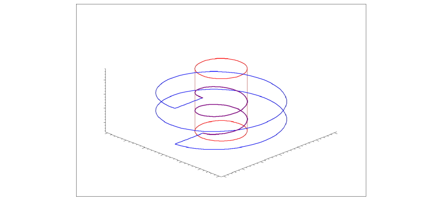
Figure 1: A cylinder of constant $H$ intersects a helical ramp of constant Re $G$ to define a trajectory.

Since a determinant is unaffected under combination of its columns, the 4-NB in eqn (10) is the same when the extraneous coordinate $p_{y}$ is introduced into a modification, $\tilde{H}\equiv H+p_{y}$, (so that $\{\tilde{H},G\}=0=\{\tilde{H},p_{y}\}$.) Then, by eqn (11),

$${df\over dt}=\{f,\tilde{H}\},$$ (14)

and so yields a superintegrable Hamiltonian system.

By contrast, suppose one took instead,

$$\tilde{H}={p_{x}^{2}+x^{2}\over 2}+p_{y}~{},\quad\tilde{G}=(p_{x}+ix)\exp(-iy)~{},$$ (15)

hence

$${df\over dt}=-i\tilde{G}\{f,\tilde{H}\}=-i\{\tilde{G}f,\tilde{H}\},$$ (16)

which is not a Hamiltonian system. For a Hamiltonian system, the four Hamilton’s equations have 6 cross-consistency conditions among them. For this system, though, even though $\nabla\cdot{\bf v}=0$, nevertheless

$$\partial_{x}\dot{x}+\partial_{p_{x}}\dot{p}_{x}-\partial_{y}\dot{y}-\partial_{p_{y}}\dot{p}_{y}=2\tilde{G}\neq 0,$$ (17)

in violation of Hamiltonian consistency. The trajectories in phase space are the same as above, but the speed along each trajectory depends on the value of $\tilde{G}$ on that trajectory.

The evolution (16) in this auxiliary phase space specifies a non-flat Poisson structure, ${\stackrel{{\scriptstyle\leftarrow}}{{\partial}}_{i}}\alpha^{ij}{\stackrel{{\scriptstyle\rightarrow}}{{\partial}}_{j}}$ (which satisfies the Jacobi identity,[16] hence $d(\alpha^{-1})=0$). Such Poisson manifolds are defined in general for all[16] NB evolution laws (12). Like the curved Poisson manifold evolutions of constrained Hamiltonian systems in $2p$-dim phase space discussed earlier, these flows could also be quantized in phase space, in principle, by Kontsevich’s[12] elaborate deformation algorithm leading to Moyal brackets (which also satisfy the Jacobi identity). In general, it is not evident that such results do not differ from those of the methods considered here.

We will consider in the next section quantization of NB evolutions simplifying through PB resolutions into

$${df\over dt}=V\{f,I_{1},...,I_{2n-1}\}=W\{f,H\},$$ (18)

for some functions $H(I_{i}),V(I_{i}),W(I_{i})$. $W$=constant (e.g. eqn (14)) amounts to maximally superintegrable Hamiltonian systems, quantized and illustrated extensively in Refs sphere,CQNB,talks.

Classically, by linearity in all derivatives involved, all three members of this equation are derivations, i.e. satisfy Leibniz’s rule,   $\delta(fg)=\delta(f)~{}g+f~{}\delta(g)$.

By contrast, eqn (16) has $V=1,W=-i\tilde{G}$. To be sure, $W\neq$const systems might well be convertible to hamiltonian ones, by virtue of non-canonical transformations—necessarily, if the hamiltonian structure is not to be preserved. E.g., for the system (15), the four equations of motion resulting from (16) can be rewritten through the change of variables,

$$p_{w}\equiv\tilde{G},\qquad w\equiv iy~{}\frac{p_{x}^{2}+x^{2}}{2\tilde{G}}~{},$$ (19)

to

$$\dot{x}=p_{x}p_{w}~{},\qquad\dot{p}_{x}=-xp_{w}~{},\qquad\dot{p}_{w}=0~{},\qquad\dot{w}=\frac{p_{x}^{2}+x^{2}}{2}~{},$$ (20)

which are derivable from a Hamiltonian, $~{}{\mathcal{H}}=p_{w}(p_{x}^{2}+x^{2})/2$.

2 Quantum Nambu Dynamics

To quantize eqn (18), we seek a map to operators in Hilbert space corresponding conventionally to the classical quantities, which preserves as much of the structure and the symmetries of it as possible,[3] or, equivalently, a deformation in phase space relying on a $\star$-product which acts on the same phase-space functions.[2] (When $W$=constant, the answer must coincide with results provided by Hamiltonian quantization.) We have found that several consistency complications are not debilitating.

Let us adopt Nambu’s proposal[1] of a fully antisymmetric multilinear generalization of Heisenberg commutators, now called quantum NBs (QNB):

$$\left[A,B\right]\equiv AB-BA,$$ (21)

$$\left[A,B,C\right]\equiv ABC-ACB+BCA-BAC+CAB-CBA,$$ (22)

$$\left[A,B,C,D\right]\equiv A[B,C,D]-B\left[C,D,A\right]+C\left[D,A,B\right]-D\left[A,B,C\right]\qquad\qquad$$ (23)

$$=[A,B][C,D]+[A,C][D,B]+[A,D][B,C]$$

$$+[C,D][A,B]+[D,B][A,C]+[B,C][A,D]~{},$$

etc. As for classical NBs, all even-QNBs resolve into strings of commutators,[3] with all suitable inequivalent orderings required for full antisymmetry, ($\propto\epsilon^{ijkl...}[I_{i},I_{j}]~{}[I_{k},I_{l}]...$): a “quantum Pfaffian”. Consequently, they manifestly have the proper classical limit[3] to the classical NBs of the previous section,

$$[I_{1},...,I_{2n}]~{}~{}\rightarrow~{}~{}n!~{}(i\hbar)^{n}~{}\{I_{1},...,I_{2n}\}.$$ (24)

By contrast, odd-QNBs have a bad classical limit, underlying our conversion to even-NBs at the classical level, (10). Thus, e.g., taking $f=p_{y}$ and eqn (13), it is easy to see that a naive quantum counterpart of (10) fails,

$$[f,H,G,p_{y}]\neq\text{const }[f,H,G].$$ (25)

It is the 4-QNB on the left-hand side which we choose for quantization below, and its even generalizations throughout. Even though the extraneous variable $p_{y}$ does not enter in the description of the classical trajectories, its operator counterpart is unavoidable in Hilbert space, as it is the commutator conjugate to the operator $y$.

A further complication of odd-QNBs[1] is also remedied by the odd-to-even embedding adopted. In quantizing (18), if the dynamical variable (whose time evolution involves its entering in a QNB) is taken to be the identity operator (e.g. $f\propto{1\kern-3.6pt\hbox to0.0pt{\hss~{}}1}$), its time derivative vanishes. Whereas, e.g. for eqn (22),

$$[{1\kern-3.6pt\hbox to0.0pt{\hss~{}}1},B,C]=[B,C]\neq 0~{},$$ (26)

which restricts the specification of $df/dt$ through odd QNBs, in general.

In contrast, this does result in the vanishing of all even-QNBs, identically, such as (23), by virtue of their commutator resolution,

$$[{1\kern-3.6pt\hbox to0.0pt{\hss~{}}1},I_{1},...,I_{2n-1}]=0~{}.$$ (27)

For other aspects of this odd-even dimorphism see Refs Hanlon,Azcarraga,CQNB.

The associative strings of operators making up the $2n$-QNBs, satisfy the proper fully antisymmetric Generalized Jacobi Identity.[19, 18, 3] E.g., for 4-QNBs, (23),

$$\epsilon^{ijklmnr}[[I_{i},I_{j},I_{k},I_{l}],I_{m},I_{n},I_{r}]=0.$$ (28)

However, the above $2n$-QNBs forfeit Leibniz’s derivation property (beyond the quantum commutator, the 2-QNB), in general. As a result, they do not satisfy the classical identities arising from the derivation property (sometimes referred to as “fundamental identities”;[20, 8] for the above 4-QNBs, those would have 5, instead of the above $7!/4!3!=35$ terms.) This may only be a subjective shortcoming, dependent on the specific application context: if a choice is forced, associativity trumps the derivation property.[18]

For example, in several Hamiltonian maximally superintegrable physical systems,[2, 3, 4] with $W$=constant, and arbitrary $V$ in eqn (18), quantization was demonstrated explicitly to be consistent. The QNBs failure to be a derivation is in accord with its being equal to operator expressions corresponding to the classical quantities

$${1\over V}{df\over dt}~{}.$$ (29)

Upon quantization, such expressions involve entwinements of derivatives of operators $df/dt$ with other operators, such as

$${1\over V}{df\over dt}+{df\over dt}{1\over V}~{}~{},$$ (30)

but often with longer, more involved strings of operators.[3] Such strings also fail to be derivations, although they can be demonstrated to provide consistent results equivalent to Hamiltonian quantization. The formal Jordan-Kurosh spectral problem[21] involving such long associative operator strings may be involved technically, but yields consistent answers.[3]

Of course, in exceptional cases (such as those with $W$=const, $V$=const), $2n$-QNBs can be derivations, if only because they are equivalent to quantum commutators. For example, quantization of eqn (14) by (25) trivially yields, by the commutator resolution (23),

$${df\over dt}=-{1\over 2\hbar^{2}}[f,H,G,p_{y}]={1\over i\hbar}[f,\tilde{H}],$$ (31)

where the operator $p_{y}$ corresponding to the extraneous variable is now featured in the effective hamiltonian. (The eigenstates of $\tilde{H}$ are thus $\psi(x,y,n,k)\propto H_{n}(x/\sqrt{\hbar})~{}\exp(iky-x^{2}/\hbar)$.)

Our conclusion, then, is that the embedding of odd to even brackets of rank one higher enables the corresponding membranes to rely on the consistent results on even-QNBs, as described, for their quantization. The toolbox provided in Ref CQNB may guide quantization of more general systems beyond Hamiltonian ones, i.e. systems with nontrivial $W$. A further important question is whether the results (such as spectra) of the QNB quantization discussed here coincide with those obtained from simple systems quantized through Kontsevich’s product—but in those cases explicit answers are normally hard to come by.

Appendix A Solenoidal Flow

Preservation of phase-space volume through solenoidal flow, $\nabla\cdot{\bf v}=0$, (Liouville’s theorem) was a guiding principle for Nambu,[1] who confirmed it for the classical dynamics of his original maximal NB. We show that all flows generated by NBs, even submaximal ones, are solenoidal, but, in general, the ones formally generated by QNBs are not.

For even classical maximal brackets in $2n$-dimensional phase space, it was made evident for (12) that $\nabla\cdot{\bf v}=0$, since

$$v^{i_{1}}=\left\{z^{i_{1}},I_{1},\cdots,I_{2n-1}\right\}=\epsilon^{i_{1}\cdots i_{2n}}~{}\partial_{i_{2}}I_{1}\cdots\partial_{i_{2n}}I_{2n-1}.$$ (A.32)

Even sub-maximal NBs are obtained from maximal ones for $2k-1$ fixed $I$s with $k<n$, through symplectic tracing of maximal brackets,[3]

$$\left\{z^{j},I_{1},\cdots,I_{2k-1}\right\}$$

$$= \frac{1}{\left(n-k\right)!}\sum_{\text{all }i=1}^{n}\left\{z^{j},I_{1},\cdots,I_{2k-1},x_{i_{1}},p_{i_{1},}\cdots,x_{i_{n-k}},p_{i_{n-k}}\right\}.$$

Hence, since each term in the sum produces a solenoidal flow, the sum of terms is also solenoidal, ${\partial_{j}}~{}\left\{z^{j},I_{1},\cdots,I_{2k-1}\right\}=0$.

Odd-NBs are obtainable through the embedding conversion described, and can likewise be made submaximal, hence they generate solenoidal flows as well,

$$0 = \partial_{j}\left\{z^{j},I_{1},\cdots,I_{2k-2}\right\}$$

$$\equiv \frac{1}{\left(n-k\right)!}\sum_{\text{all }i=1}^{n}\partial_{j}\left\{z^{j},I_{1},\cdots,I_{2k-2},x_{i_{1}},p_{i_{1},}\cdots,x_{i_{n-k}},p_{i_{n-k}},p_{2n}\right\}.$$

The direct quantum operator analog of the above classical $\nabla\cdot{\bf v}$ (reducing to it in the classical limit) is

$$K(I_{i},...)\equiv J_{ij}[z^{i},[z^{j},I_{1},I_{2},\cdots]],$$ (A.35)

where $J_{ij}$ is the standard symplectic metric for the canonical variables, $[z^{i},z^{j}]=i\hbar J_{ij}$. In general, $K$ does not vanish, even though in special circumstances, such as (15), it can vanish. That is, e.g. for 3-QNBs,

$$K=J_{ij}[z^{i},[z^{j},H,G]]=\frac{1}{2}J_{ij}~{}[z^{i},z^{j},H,G]-J_{ij}z^{i}[z^{j},[H,G]]~{}.$$ (A.36)

For $\tilde{H}$ and $\tilde{G}$, both their commutator and the quantum symplectic trace ($J_{ij}[z^{i},z^{j},\tilde{H},\tilde{G}]]=0$) vanish.

In general, however, even for privileged flows for which $\left[H,G\right]=0$ (so that they leave the unit operator invariant, by eqn (26):   $[{1\kern-3.6pt\hbox to0.0pt{\hss~{}}1},H,G]=[H,G]=0$), the above symplectic trace is non-vanishing, as can be seen by taking brackets of exponentials linear in the canonical variables:

$$J_{lj} \Bigl{[}z^{l},z^{j},\exp\left(i\alpha\cdot z\right),\exp\left(i\beta\cdot z\right)\Bigr{]}$$

$$= i\hbar\left(4n-\frac{2\hbar\alpha\wedge\beta}{\tan\left(\frac{\hslash}{2}\alpha\wedge\beta\right)}\right)~{}\Bigl{[}\exp\left(i\alpha\cdot z\right),\exp\left(i\beta\cdot z\right)\Bigr{]}~{},$$

where $\alpha\wedge\beta\equiv\alpha^{i}J_{ij}\beta^{j}$. Operator Fourier analysis of general $H$ and $G$ evinces the quantum symplectic trace to not be necessarily proportional to $[H,G]$.

In general, $K$ reduces to the antisymmetric derivator[3] for canonical variables. The derivator for any given string of $A$s is defined for all $B$ and $C$ as

$$( B ,C\ |\ A_{1},\cdots,A_{k})$$

$$\equiv \left[BC,A_{1},\cdots,A_{k}\right]-B\left[C,A_{1},\cdots,A_{k}\right]-\left[B,A_{1},\cdots,A_{k}\right]C,$$

so that it vanishes for all $B$ and $C$ iff the $(k+1)$-QNB-generated action of the string of $A$s is a derivation.

A sufficient condition for formal “operator solenoidal flow” follows from the identity,

$$J_{ij} \left[z^{i},\left[z^{j},A_{1},\cdots,A_{k}\right]\right]$$

$$= i\hbar n~{}[{1\kern-3.6pt\hbox to0.0pt{\hss~{}}1},A_{1},\cdots,A_{k}]-J_{ij}\ \left(z^{i},z^{j}\ |\ A_{1},\cdots,A_{k}\right).$$

For even $k+1\equiv 2m$, by eqn (27), the first term on the r.h.s. drops out, and $K$ amounts to minus the derivator.

For odd QNBs, even $k=2m$, as for (26), $\left[{1\kern-3.6pt\hbox to0.0pt{\hss~{}}1},A_{1},\cdots,A_{2m}\right]=\left[A_{1},\cdots,A_{2m}\right]$ may not vanish in general, but one might consider the privileged “flows” for which it does. Thus, for such privileged odd-QNB-generated operator flows and for all even-QNB-generated flows,

$$K=J_{ij}\ \left[z^{i},\left[z^{j},A_{1},\cdots,A_{k}\right]\right]=-J_{ij}~{}\left(z^{i},z^{j}\ |\ A_{1},\cdots,A_{k}\right).$$ (A.40)

Quantum flows are thus solenoidal if the action of the $A_{1},\cdots,A_{k}$ in an $(k+1)$-QNB is a derivation.

However, it is not necessary for the general derivator to vanish to have operator solenoidal flow—just this particular derivator. For the example considered above, $\tilde{H}$, $\tilde{G}$, a 3-QNB based on them is not a derivation, in general:  $\left(B,C\ |\ \tilde{H},\tilde{G}\right)\neq 0$ for all $B$ and $C$. Nonetheless, as noted, $K$ vanishes for this case, as well as for the 3-QNB system with $\tilde{H},G$, eqs (13, 15), and the 4-QNB system with $\tilde{H},\tilde{G},p_{y}$, eqs (13, 31).

References

- [1] Y Nambu, Phys Rev D7, 2405-2412 (1973).
- [2] T Curtright and C Zachos, New J Phys 4, 83.1-83.16 (2002) [hep-th/0205063].
- [3] T Curtright and C Zachos, Phys Rev D68, 085001 (2003) [hep-th/0212267].
- [4] T Curtright and C Zachos, Short Distance Behavior of Fundamental Interactions: 31st Coral Gables Conference on High Energy Physics and Cosmology, B Kursunoglu et al, eds, (AIP Conference Proceedings 672, 2003) pp 165-182 [hep-th/0303088]; C Zachos, Phys Lett B570, 82-88 (2003) [hep-th/0306222]; T Curtright, [hep-th/0307121].
- [5] F Estabrook, Phys Rev 8, 2740-2743 (1973).
- [6] M Rasetti and T Regge, Physica 80A, 217-233 (1975).
- [7] F Lund and T Regge, Phys Rev D14, 1524-1535 (1976).
- [8] L Takhtajan, Commun Math Phys 160, 295-316 (1994).
- [9] P A M Dirac, Can J Math 3, 1 (1951); Lectures on Quantum Mechanics, Yeshiva University 1964 (reprinted by Dover, 2001).
- [10] N Mukunda and E Sudarshan, Phys Rev D13, 2846-2850 (1976).
-
[11]
F Bayen and M Flato, Phys Rev D11, 3049-3053
(1975);
A Kálnay and R Tascón, Phys Rev D17, 1552-1562 (1978). - [12] M Kontsevich (1997) [q-alg/9709040].
- [13] R Bryant, S Chern, R Gardner, H Goldschmidt, and P Griffiths, Exterior differential systems (Springer-Verlag, New York, 1991).
-
[14]
Y Matsuo and Y Shibusa, JHEP02, 006 (2001)
[hep-th/0010040];
A Speliotopoulos, J Phys A35, 8859-8866 (2002). -
[15]
B Pioline, Phys Rev D66, 025010 (2002);
D Minic and C-H Tze, Phys Lett B536, 305-314 (2002) [hep-th/0202173];
C Hofman and J-S Park, [hep-th/0209148];
S Pandit and A Gangal, J Phys A31, 2899-2912 (1998);
D Fairlie and T Ueno, J Phys A34, 3037 (2001) [hep-th/0011076];
I Bengtsson, N Barros e Sá, and M Zabzine, Phys Rev D62 (2000) 066005 [hep-th/0005092]. - [16] C Gonera and Y Nutku, Phys Lett A285, 301-306 (2001); Y Nutku, J Phys A36, 7559-7567 (2003) [quant-ph/0306059].
-
[17]
R Chatterjee, Lett Math Phys 36, 117-126
(1996);
A Teğmen and A Verçin, [math-ph/0212070]. - [18] J de Azcárraga, A Perelomov, and J Pérez Bueno, J Phys A29, 7993-8010 (1996) [hep-th/9605067]; J de Azcárraga, and J Pérez Bueno, Commun Math Phys 184, 669-681 (1997) [hep-th/9605213]; J de Azcárraga, J Izquierdo, and J Pérez Bueno, J Phys A30, L607-L616 (1997) [hep-th/9703019]; Rev R Acad Cien Serie A Mat 95, 225-248 (2001) [physics/9803046].
- [19] P Hanlon and M Wachs, Adv Math 113, 206-236 (1995).
-
[20]
V T Filippov, Sib Math Jou, 26, 879-891 (1985);
D Sahoo and M Valsakumar, Phys Rev A46, 4410-4412 (1992); Mod Phys Lett A9, 2727-2732 (1994);
J Hoppe, Helv Phys Acta 70, 302-317 (1997) [hep-th/9602020]. - [21] A G Kurosh, Russian Math Surveys 24, 1-13 (1969).