HU-EP-03/85 ; DFPD 03/TH 48

Loop Equation in Two-dimensional
Noncommutative Yang-Mills Theory

Harald Dorn
Institut für Physik, Humboldt-Universität zu Berlin
Newtonstr. 15, D-12489 Berlin, Germany
Alessandro Torrielli
Dipartimento di Fisica “G. Galilei”, INFN Sezione di Padova
Via Marzolo 8, 35131 Padova, Italy

Abstract

The classical analysis of Kazakov and Kostov of the Makeenko-Migdal loop equation in two-dimensional gauge theory leads to usual partial differential equations with respect to the areas of windows formed by the loop. We extend this treatment to the case of $U(N)$ Yang-Mills defined on the noncommutative plane. We deal with all the subtleties which arise in their two-dimensional geometric procedure, using where needed results from the perturbative computations of the noncommutative Wilson loop available in the literature. The open Wilson line contribution present in the non-commutative version of the loop equation drops out in the resulting usual differential equations. These equations for all $N$ have the same form as in the commutative case for $N\rightarrow\infty$. However, the additional supplementary input from factorization properties allowing to solve the equations in the commutative case is no longer valid.

1 Introduction

The loop equation has been the subject of a deep study in the literature, since the very beginning of its formulation [1, 2, 3, 4]. It is an evolution equation for a class of gauge invariant operators of gauge theory, the Wilson loop observables, which are considered to be the basic dynamical objects of the theory: in the confining phase, the knowledge of these colorless averages determines all the information. The solution of this loop equation should therefore provide the essential dynamics of the quantum gauge theory. The right hand side of the equation is given by an insertion of the Yang-Mills equation of motion operator into the Wilson loop. The so-called loop operator on the left hand side is constructed out of suitable second order variational derivatives with respect to the contour of the Wilson loop. In the formulation following Polyakov it is given by some projection applied to the standard second variational derivative, for a more recent version see [5]. In the Makeenko-Migdal approach it is given by a construction involving the so-called area derivative.

The equation contains singularities, which are connected both with the usual problem of renormalization of short distance divergences in multi-point Green functions as well as with the restriction of D-dimensional distributions to the one-dimensional contour of the Wilson loop. The precise form of the equation for the renormalized theory is a delicate issue and the related problems are not completely solved. There are at least strong arguments that the standard first and second variational derivation can be interchanged with the renormalization procedure [6]. But due to the short distance singularities of two insertions for first order variation [6, 5] the projection recipe [5] for the loop operator becomes difficult to handle for practical calculations. On the other side the area derivative is less well behaved under renormalization.

Gauge theories in two dimensions have a long history serving as a testing area for problems more complicated in four dimensions. Also in the context of loop equations the situation becomes better in two dimensions. Here a renormalized version of the Makeenko-Migdal equation has been derived by Kazakov and Kostov [7]. An important advantage of their equation is the reduction to an usual partial differential equation with respect to the areas of the windows formed by a general 2-dimensional loop with intersections. They were also able to solve the equation in the large $N$-limit. In addition for some set of loops solutions have been obtained for generic $N$, [8]. Remarkably, from their solution one can derive an expression for Wilson loops winding $n$ times around a single patch [9], which coincides with the one obtained via other methods, such as lattice [10], or geometric means [11, 12], or light-cone gauge perturbation theory with ’t Hooft’s prescription. In connection with this solution, it was possible to understand instanton contributions to determine the area-law, and many features of the light-cone perturbative expansion [13].

More recently, noncommutative gauge theories have received attention carrying a new idea of physics at short length, essentially based on their tight relation to string theory. In this context, new issues arise for gauge theories, especially the merging of space-time transformation and gauge symmetries in a larger group, and new classes of instanton solutions. An important discovery was that in these theories, new gauge invariant observables come together with the Wilson loops, the so-called noncommutative open Wilson lines [14]. We have therefore a larger set of candidates to encode the full dynamical content of the theory. The noncommutative generalization of the Makeenko-Migdal equation was found in [15, 16] for a gauge group $U(N)$

$$\partial^{\mu}{{\delta}\over{\delta\sigma^{\mu\nu}(\xi)}}{{\langle W_{c}[C]\rangle}\over{V}} = -{{g^{2}N}\over{V^{2}}}\int_{C}d\eta_{\nu}~{}\delta^{(D)}(\xi-\eta)\langle W_{c}[C_{\xi\eta}]\rangle\langle W_{c}[C_{\eta\xi}]\rangle$$ (1)

$$- {{g^{2}N}\over{{(2\pi)}^{D}V\det\theta}}\int_{C}d\eta_{\nu}{\langle W_{o}[C_{\xi\eta}]W_{o}[C_{\eta\xi}]\rangle}_{\mbox{\scriptsize conn}}~{}.$$

The closed Wilson loop is defined as

$$W_{c}[C]=\int dx{{1}\over{N}}\,\mbox{Tr}\,U[x+C]~{},$$ (2)

$$U[C]=P_{\star}\exp\Big{(}i\int_{C}A_{\mu}(\xi(\tau))d\xi^{\mu}(\tau)\Big{)}~{},$$ (3)

while the open lines are

$$W_{o}[C]=\int dx{{1}\over{N}}\,\mbox{Tr}\,U[x+C]\star e^{-ik_{\xi}x}~{},$$ (4)

where $k_{\xi}={\theta}^{-1}(\xi(1)-\xi(0))$ in order to ensure gauge invariance [14]. V is the volume of space-time, and we assume the matrix $\theta$ to be nondegenerate.

One realizes that it contains a term which involves also the gauge-invariant open Wilson lines. Moreover, it reproduces the singular nature of the traditional loop equation with the appearance of the delta function in the factorized part, so it is natural to ask if going down to two-dimensions, it will be again possible to give it a regular form. In the noncommutative case the comparison still cannot be performed with exact geometric expressions for the loop, but one can compare for instance with the lattice [17, 18], and with the large amount of calculations that have been done in noncommutative light-cone perturbation theory [19, 20, 21]. Concerning this last case, the results are summarized in the following.

When using light-cone gauge in two dimensions, there are two different prescriptions for the pole of the propagator that one can use: one is ’t Hooft’s one [22], which in the commutative case leads to a resummation of the perturbative series of the Wilson loop which coincides with the nonperturbative expression, and which exhibits the area law. Another possible prescription is WML’s one [24, 25, 26], which is purely perturbative. The two-dimensional Wilson loop treated with the WML’s prescription can be shown to reproduce actually only the zero-instanton sector of the complete result [27], and leads to a resummed expression which consists of exponential times polynomials in the area [28]. Pure area dependence is ensured by the invariance of the theory under area-preserving diffeomorphisms [29].

In the noncommutative case, the loop computed with ’t Hooft’s prescription turns out to be ill-defined [19]. The loop computed with WML’s prescription is instead finite, with a finite limit different from zero at large noncommutativity and a continuous but non-analytic behaviour when the noncommutativity goes to zero.

Our aim is to repeat the way to the two-dimensional Kazakov-Kostov version of the Makeenko-Migdal equation in the light of these results. We will find that it is still possible, following the same line of reasoning, to arrive at a regular version of the equation, which is actually a series of relation among loops in a wide class of different contours. We will use the input of the explicit Feynman diagrams computations and we will deal with the subtleties of the derivation in the noncommutative setting. Remarkably, we realize that in the final version of the equation the contribution from the open lines is no more present. Moreover, the final form of the equation turns out to be the same as the commutative one in the large-$N$ limit, but valid for generic $N$, and generic $\theta$. At a first glance this could sound quite surprising, since the perturbative computations show that the noncommutative Wilson loop is likely to be very different in general from the large $N$ commutative one. The point is that still the kind of supplementary equation one would write in order to find an explicit solution should be drastically different. The meaning of the final form of the un-supplemented equation can be to put constraints on the perturbative expansion, either on WML’s result or constraining eventual renormalization coefficients introduced in order to give a meaning to the Wilson loop with ’t Hooft propagator. On the other side the equation provides a relation directly for exact loop quantum averages, as they can be derived by nonperturbative means. This opens the perspective of a more powerful test of our equation which challenges the current available nonperturbative techniques [30, 31, 32, 33, 34, 35, 17, 18].

2 Sketch of the Kazakov-Kostov analysis

Since we will closely follow the classical Kazakov-Kostov derivation of the two-dimensional regular loop equation, we report here for convenience its main points.

The first step is to take the expression for the Wilson loop quantum average and to perform the area-derivative ${{\delta}/{\delta\sigma^{\mu\nu}(\xi)}}$ (for a detailed explanation, see [36]). This means one takes the variation of the loop functional when adding a small loop to the contour with infinitesimal area at the point $\xi$ on the contour. One then keeps the contributions linear in the small area. Among these contributions, there is a first term which reproduces as usual the field-strength via the Stokes theorem, and that is all on the classical level. In the quantum case and in the special setting of two dimensions one has a further contribution instead. Namely,

$$\delta W_{c}[C]={{i}\over{2N}}\langle\,\mbox{Tr}\,P\Big{[}F_{\mu\nu}(\xi)\exp\Big{(}i\int_{C}A_{\mu}(\xi(\tau))\,d\xi^{\mu}(\tau)\Big{)}\Big{]}\rangle\,\delta\sigma^{\mu\nu}$$

$$-{{1}\over{2N}}\langle\,\mbox{Tr}\,\Big{[}{\Big{(}\int_{\delta C}A_{\mu}(\xi(\tau))\,d\xi^{\mu}(\tau)\Big{)}}^{2}P\exp\Big{(}i\int_{C}A_{\mu}(\xi(\tau))\,d\xi^{\mu}(\tau)\Big{)}\Big{]}\rangle$$

$$+{\cal{O}}({\delta\sigma^{2}})~{}.$$ (5)

Computing the contribution to the variation coming from the two point function integrated around the small added loop as in (2), see fig.1, one finds a linear dependence on $\delta\sigma^{\mu\nu}$, which is peculiar to two dimensions.

Figure 1: A single propagator inserted in the small loop

Then, one takes the point-derivative $\partial^{\mu}$ with respect to the position $\xi$ of the previous insertion. The first term in (2) turns as usual into the covariant derivative of the field-strength, and it is the way in which one can insert the quantum dynamics: using the quantum equation of motion one turns this term into an integral along the contour of a two-dimensional delta function, times the correlator of the two parts in which the contour is divided by the insertion point $\xi$ and an integration point $\eta$:

$$-g^{2}N\int_{C}d\eta_{\nu}\,\delta^{(2)}(\xi(\tau_{0})-\eta(\tau))~{}\langle W_{c}[C_{\xi\eta}]W_{c}[C_{\eta\xi}]\rangle~{}.$$ (6)

The extra term from (2) contains now the derivative of the normalized tensor which defines the small area $\delta\sigma^{\mu\nu}$, which is basically a sign when changing the orientation; therefore it produces a delta function contribution. This exactly cancels the contribution coming from the first term (6) at the trivial coincidence point $\tau=\tau_{0}$. What remains is the contribution in (6) due to the other value (we assume unique) of the parameter $\tau$ for which it happens that $\xi(\tau_{0})=\eta(\tau)$. This residual term after integration along the contour still contains a one-dimensional delta function with respect to the orthogonal direction to the contour. To produce a finite expression one integrates along a small path of infinitesimal length $2\Delta$ intersecting the contour $C$ at $\xi$. This results in the equation

$$\lim_{|\Delta|\to 0}[\delta/|\delta\sigma(\xi+\Delta)|-\delta/|\delta\sigma(\xi-\Delta)|]~{}\langle W_{c}[C]\rangle$$

$$=-g^{2}N~{}\langle W_{c}[C_{1}]W_{c}[C_{2}]\rangle~{},$$ (7)

if $\xi$ is a (simple) self-intersection point and $C_{1}$ and $C_{2}$ are the two closed parts in which it divides $C$. If $\xi$ is not a self-intersection point, the r.h.s of (2) is zero. When taking the large-$N$ limit, the correlator of the two loops in (2) factorizes in the product of two single quantum averages.

Eq.(2) is now in a regular form: assuming the loop functionals with many windows to be functions of the areas of these windows alone, due to the above mentioned symmetry under area-preserving diffeomorphisms, it can be turned into a system of partial differential equations for these functions, of the first order in the derivatives with respect to the areas of the windows:

$$\Big{(}\frac{\partial}{\partial S_{k}}+\frac{\partial}{\partial S_{i}}-\frac{\partial}{\partial S_{l}}-\frac{\partial}{\partial S_{j}}\Big{)}~{}\langle W_{c}[C]\rangle~{}=~{}-g^{2}N\langle W_{c}[C_{1}]W_{c}[C_{2}]\rangle~{}.$$ (8)

It can be represented graphically as in fig.2.

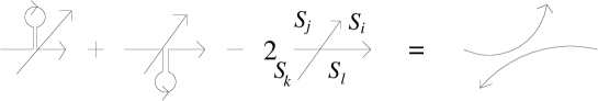
Figure 2: Graphical representation of the final equation

Supplementing it with some other assumptions that are justified on the basis of geometrical factorization properties, and on the exponentiation of the simple loop with one window, in the limit of large $N$ (when $\langle W_{c}[C_{1}]W_{c}[C_{2}]\rangle=\langle W_{c}[C_{1}]\rangle\langle W_{c}[C_{2}]\rangle$) one can completely determine the system [7], and the results reproduce ’t Hooft’s resummed perturbation theory. These factorization assumptions are not valid for WML’s prescription, for which perhaps different supplementary equations could work together with (8).

3 The Noncommutative Computation

In this section, we repeat the kind of analysis that Kazakov-Kostov did now in the noncommutative setting. We still assume that acting on the noncommutative Wilson loop with $\partial^{\mu}{{\delta}\over{\delta\sigma^{\mu\nu}}}$ is a well defined operation (in other words, that it is a functional of the Stokes type). In the commutative case this was guaranteed by the pure area dependence due to invariance under area-preserving diffeomorphisms. This survives in the noncommutative setting. Supports to this assumption come from the fact that for example all the explicit computations performed in [19, 20, 21] show that the Wilson loop averages depend only on the area of the contour. Invariance under area-preserving diffeomorphisms is actually believed to be one of the main ingredient of the structure of the noncommutative gauge group in two dimensions [37, 38, 39].

We will use the light-cone gauge fixing $A_{-}=0$ and allow in parallel both the WML’s and ’t Hooft’s prescription for the propagator. In [19] (see also [21]) it was shown that ’t Hooft’s prescription leads to a series of problems originating from the occurrence of products of distributions which are ill-defined, and resulting in some divergences in the perturbative expansion. It was thought that the origin of this fact, when compared with the finite commutative result, and with the smooth expression one gets using instead WML’s prescription as shown in [19, 20, 21], could be perhaps attributed to an incompatibility of the punctual interaction that characterises ’t Hooft’s propagator with the noncommutativity of the space-time. All the evidence was then towards avoiding ’t Hooft’s prescription. Instead, we will take for it another point of view: we take the approach of renormalization of singularities. We therefore assume that the Wilson loop, when treated with ’t Hooft’s prescription, is however regularized in some way in order to have a finite result, and also renormalized through some subtraction procedure, which leaves it of the Stokes type.

3.1 Variation of the Wilson Loop

In repeating the Kazakov-Kostov analysis we start evaluating the area variation of the functional $W_{c}[C]$. This means we write

$${{1}\over{V}}W_{c}[C\delta C] = {{1}\over{V}}\langle\int dx{{1}\over{N}}\,\mbox{Tr}\,P_{\star}\Big{[}\exp\Big{(}i\int_{\delta C}A_{\mu}(x+\xi(\tau))d\xi^{\mu}(\tau)\Big{)}$$ (9)

$$\star\,\exp\Big{(}i\int_{C}A_{\mu}(x+\xi(\tau))d\xi^{\mu}(\tau)\Big{)}\Big{]}\rangle~{},$$

where $\delta C$ is a small loop of area $\delta\sigma^{\mu\nu}$ we add to the original contour $C$ at the point $\xi$ in such a way that drawing $\delta C$ does not add new self-intersections [7]. We will consider the same class of contours considered in [7] i.e. with an arbitrary number of simple self-intersections. According to the previous considerations, we still assume that the corresponding Wilson loops depend only on the areas of the windows in which the various self-intersections divide the contour. Expanding the contribution from the $\delta C$-integration in powers of the gauge field as in [7], we single out a first term that reproduces the original Wilson loop, a second term linear in the gauge field on $\delta C$ which is treated in the usual way making use of Stokes’ theorem, and then a tower of contributions containing one or more propagators inside the small loop $\delta C$ or more than two propagators connecting $\delta C$ with $C$. Among these, we should keep only the ones at most linear in $\delta\sigma^{\mu\nu}$. In the commutative case this amounts to a single term coming from the two-point function of gauge fields both on the small loop. The corresponding term is now with analogous considerations

$$-~{}{{1}\over{2V}}\int dx{{1}\over{N}}\,\mbox{Tr}\,\Big{[}\langle\int_{\delta C}\int_{\delta C}A_{\mu}(x+\xi(\tau))\star A_{\nu}(x+\xi(\tau^{\prime}))~{}d\xi^{\mu}(\tau)d\xi^{\nu}(\tau^{\prime})\rangle$$

$$\star\,\langle P_{\star}\exp\Big{(}i\int_{C}A_{\mu}(x+\xi(\tau))d\xi^{\mu}(\tau)\Big{)}\rangle\Big{]}~{}.~{}~{}~{}~{}~{}$$ (10)

For this term one can use that quantum averages are indeed invariant under translations [15], therefore the two quantum averages in Eq.(3.1) are independent of $x$. We can bring the first one outside the integral over $dx$. Moreover, this first quantum average is unaffected by the noncommutativity, which starts acting when diagrams with crossing propagators enter the game [19, 21]. Using also that the two-point correlator of the gauge field is diagonal in color space, we see that (3.1) amounts to the product of ${{1}\over{V}}\langle W_{c}[C]\rangle$ times the same coefficient $(-{{1}\over{2}})\int_{\delta C}\int_{\delta C}D_{++}(\xi(\tau)-\xi(\tau^{\prime}))$ as in the commutative case. There, this was the only contribution linear in the small area $|\delta\sigma|$ beyond the $F$-insertion term. Kazakov and Kostov used in particular that Green’s function with more than two gauge fields on the small contour yield contributions higher order in $\delta\sigma^{\mu\nu}$.

This property is still true in the noncommutative case for WML [20, 21], but is no more true for ’t Hooft. Explicit calculations in [19] have shown that in the contribution from the crossed part of the four-point function to a loop with a single window of area $A$ evaluated with ’t Hooft’s propagator, one gets a finite part that can be expanded in positive powers of $1/\theta$, in which each coefficient is proportional to a power of the area larger than one, plus two terms with a positive power of $\theta$, of the form $a\theta+b\theta^{2}$. These two terms were the origin of the ill-definiteness we mentioned at the beginning, and we assume here them to be suitably regularized and renormalized. A natural assumption is that this can be done without breaking the pure area dependence, which is a requirement that the symmetry under area-preserving diffeomorphism does not produce anomalies. At the end, just by dimensional analysis one expects $b$ to be a function $f_{b}(A,\lambda)$ of a dimensionless combination of the area $A$ and of some renormalization scale $\lambda$, and $a$ to be given by the area $A$ itself times another function $f_{a}(A,\lambda)$ with dimensionless combinations. Altogether

$$a\theta+b\theta^{2}=Af_{a}(A,\lambda)\theta+f_{b}(A,\lambda)\theta^{2}.$$ (11)

These terms can in principle provide a linear dependence on the area.

We now want to make a series of important remarks. The assumption that the symmetry under area-preserving diffeomorphism is not anomalous implies that one can find at least one procedure of regularization and renormalization such that it is preserved. We have been able to find a suitable regularization in coordinate space on a rectangular contour that makes these singular terms to be actually zero, due to a loop coordinate symmetry. This is in contrast to previous treatments based on a momentum space procedure [19, 20, 21]. But as usual different treatments of such singular distributional integrals can give different results. We have arguments that this coordinate space procedure can work also at higher orders, but we are not able to put it into a theorem. However, this strongly suggests that a regularization exists that does not break at least the pure area-dependence, and in particular with this regularization $f_{a}$ and $f_{b}$ and analog terms from higher than four point functions can be zero.

In our subsequent treatment, since the regularization of this integral is such a delicate issue, we are general and allow for non-vanishing coefficients, also in order to avoid being too tight to the rectangle for these singular terms. The main point we stress here is the following: we will see that whenever non-zero, they however will not change the final form of the equation, due to a geometric constraint we will find below. The form (20) and the equations derived from it are stable against this ambiguity.

3.2 Derivation of the Equation

Green’s functions with two and in principle also more propagators on the small loop $\delta C$ can potentially provide further contributions linear in the small area $|\delta\sigma|$. In order to be general, we will write therefore the total extra contribution (i.e. additional to the field strength insertion) to the derivative ${{1}\over{V}}\partial^{\mu}{{\delta}\over{\delta\sigma^{\mu\nu}}}\langle W_{c}[C]\rangle$ as

$${{1}\over{|\delta\sigma|}}{\Bigg{[}{{\langle W_{c}[\delta C]\rangle}\over{V}}-1\Bigg{]}}_{\mbox{\scriptsize lin. in $|\delta\sigma|$ }}\partial^{\mu}n_{\mu\nu}\,{{\langle W_{c}[C]\rangle}\over{V}}~{},$$ (12)

where we have introduced a two-dimensional tensor such that ${{\delta}\over{\delta\sigma^{\mu\nu}}}=n_{\mu\nu}{{\delta}\over{|\delta\sigma|}}$, and we have used again that quantum averages are invariant under translations.

The next step is to use the result of [15] for the term corresponding to the field-strength insertion, namely the right-hand side of Eq.(1). We see that this contains a delta-like term similar to the one which commonly appears in the right-hand side of the commutative Makeenko-Migdal equation, but already factorized in the two quantum averages relative to the two sections in which the loop is divided, plus a term which contains the connected correlator of the two Wilson lines corresponding to these sections. We will consider later the piece with the Wilson lines. Restricting to the other term, it has for any generic $N$ the same form as the commutative case at $N\to\infty$. If we write it explicitly in our case it is similar to (6)

$$-{{g^{2}N}\over{V^{2}}}\int_{C}d\eta_{\nu}(\tau)~{}\delta^{(2)}(\xi(\tau_{0})-\eta(\tau))\langle W_{c}[C_{\xi\eta}]\rangle\langle W_{c}[C_{\eta\xi}]\rangle~{}.$$ (13)

If $\xi$ is not a self-intersection point, a contribution to (13) comes only from the trivial coincidence $\tau=\tau_{0}$. Otherwise there will be other contributions from the other values of the parameter $\tau$ such that $\eta(\tau)=\xi(\tau_{0})$. As in the commutative case, we can conclude that here again (3.1) cancels the trivial coincidence contribution, both for ’t Hooft and WML, since the two-point contribution is the same for simple loops. Therefore we write

$${{1}\over{V}}\partial^{\mu}{{\delta}\over{\delta\sigma^{\mu\nu}(\xi)}} \langle W_{c}[C]\rangle~{}=$$ (14)

$$-~{}{{g^{2}N}\over{V^{2}}}~{}\backslash{\hskip-9.68747pt}\int d\eta_{\nu}(\tau)~{}\delta^{(2)}(\xi(\tau_{0})-\eta(\tau)\langle W_{c}[C_{\xi\eta}]\rangle\langle W_{c}[C_{\eta\xi}]\rangle$$

$$+\Bigg{[}{{\langle W_{c}[\delta C]\rangle}\over{V}}\Bigg{]}_{\diamondsuit}~{}{{\langle W_{c}[C]\rangle}\over{V}}~{}~{}\partial^{\mu}n_{\mu\nu}~{}+~{}\mbox{Wilson lines}~{},$$

where we have defined

$${\Bigg{[}{{\langle W_{c}[\delta C]\rangle}\over{V}}\Bigg{]}}_{\diamondsuit}={{1}\over{|\delta\sigma|}}{\Bigg{[}{{\langle W_{c}[\delta C]\rangle}\over{V}}\Bigg{]}}_{\mbox{\scriptsize lin. in $|\delta\sigma|$, 4 p.t and more}}~{}.$$ (15)

The backslash on the integral in (14) indicates the omission of a small part of the contour around $\tau=\tau_{0}$. Note that $\partial^{\mu}n_{\mu\nu}$ can be rewritten as $\int_{\tau=\tau_{0}-\epsilon}^{\tau_{0}+\epsilon}d\eta_{\nu}(\tau)\delta^{(2)}(\xi(\tau_{0})-\eta(\tau))$. The corresponding term with the two-point function in the small loop was just responsible for the cancellation of the trivial coincidence contribution in the first term of the r.h.s. of (14).

We will now require that after renormalization the Wilson loop in ’t Hooft’s prescription still fulfills the basic requirement of approaching one for vanishing enclosed area. Applying this to the simple loop $\delta C$ that appears in (14) implies that the corrections we find from four and higher point functions must approach zero as $|\delta\sigma|$ goes to zero. Constant or divergent pieces as $|\delta\sigma|\to 0$, if any, must be set to zero for consistency, and this gives Eq.(14) a well defined meaning. In particular, we assume for the functions $f_{a}$ and $f_{b}$ previously introduced for the four point function (see eq.(11)), the following form:

$$f_{a}(A,\lambda)=\sum_{i=0}^{\infty}{(A/\lambda)}^{i}\,f_{a}^{i}\,\,;\,\,f_{b}(A,\lambda)=\sum_{i=1}^{\infty}{(A/\lambda)}^{i}\,f_{b}^{i}~{}.$$ (16)

Analogous requirements must be satisfied by higher order Green’s functions.

At this stage we follow Kazakov and Kostov’s strategy of eliminating the surviving delta-like singularities still present in Eq.(14). We integrate as in [7] along a small path $\delta C_{\perp}$ intersecting the contour $C$ at the point $\xi(\tau_{0})$, and then let the length of this path going to zero. What we get is the following for $\xi$ a self-intersection point:

$${{1}\over{V}}\lim_{|\Delta|\to 0}[\delta/|\delta\sigma(\xi+\Delta)|-\delta/|\delta\sigma(\xi-\Delta)|]~{}\langle W_{c}[C]\rangle=$$

$$-{{g^{2}N}\over{V^{2}}}\langle W_{c}[C_{1}]\rangle\langle W_{c}[C_{2}]\rangle~{}+~{}{\Bigg{[}{{\langle W_{c}[\delta C]\rangle}\over{V}}\Bigg{]}}_{\diamondsuit}~{}~{}{{\langle W_{c}[C]\rangle}\over{V}}$$

$$+\,\lim_{|\Delta|\to 0}\int_{\delta C_{\perp}}\mbox{Wilson lines}~{},$$ (17)

where $C_{1}$ and $C_{2}$ are the two nontrivial sections in which $\xi$ divides the original contour $C$. We give the operation on the left-hand side the same meaning as in [7], and we explicitly translate it into a sum of simple partial derivatives with respect to the areas $S_{m}$ of the four windows which meet at $\xi$ as in eq.(8).

Now we consider the same for a non self-intersecting point. We get

$${{1}\over{V}} \lim_{|\Delta|\to 0} [\delta/|\delta\sigma(\xi+\Delta)|-\delta/|\delta\sigma(\xi-\Delta)|]~{}\langle W_{c}[C]\rangle~{}=$$ (18)

$${\Bigg{[}{{\langle W_{c}[\delta C]\rangle}\over{V}}\Bigg{]}}_{\diamondsuit}~{}~{}{{\langle W_{c}[C]\rangle}\over{V}}$$

$$+~{}\lim_{|\Delta|\to 0}\int_{\delta C_{\perp}}\mbox{ Wilson lines}~{}.$$

Since by assumption $\xi$ is a non self-intersecting point, the left-hand side is zero. This means that we must require for consistency

$${\Bigg{[}{{\langle W_{c}[\delta C]\rangle}\over{V}}\Bigg{]}}_{\diamondsuit}{{\langle W_{c}[C]\rangle}\over{V}}+\Bigg{[}\,\lim_{|\Delta|\to 0}\int_{\delta C_{\perp}}\mbox{ W. lines}\Bigg{]}=0~{}.$$ (19)

In the starting loop equation (1) the open Wilson line contribution, in contrast to the first term on the r.h.s., has no evident distributional character. Therefore, we expect this term not to contribute in the limit $|\Delta|\rightarrow 0$. We comment more on this issue in the appendix and continue taking the vanishing of the Wilson line term in (19) for granted. Then also the first term in (19) has to vanish, i.e. $[\langle W_{c}[\delta C]\rangle/V]_{\diamondsuit}=0$. The last statement is independent of the point $\xi$, and using it now in (3.2) we get

$${{1}\over{V}}\Big{(}\frac{\partial}{\partial S_{k}}+\frac{\partial}{\partial S_{i}}-\frac{\partial}{\partial S_{l}}-\frac{\partial}{\partial S_{j}}\Big{)}~{}\langle W_{c}[C]\rangle~{}=-~{}{{g^{2}N}\over{V^{2}}}\langle W_{c}[C_{1}]\rangle\langle W_{c}[C_{2}]\rangle,$$ (20)

which has the same form as the commutative equation for $N\to\infty$, but it is valid for generic $N$ now.

Following the line of reasoning of Kazakov and Kostov we arrived at a non-singular version of the Makeenko-Migdal equation for the noncommutative case in two dimensions. Equation (20) is our main result and is expected to be valid also nonpertubatively.

A first remark is about the solutions of this equation. As already in the commutative case, as it stands it cannot be solved without implementing some further input. Kazakov and Kostov used results from explicit calculations with ’t Hooft’s prescription, and derived a further equation which, combined with the previous in the large $N$ factorized limit, allowed them to find an explicit solution within the ’t Hooft prescription (corresponding to the exact geometrical one). We cannot use their supplementary equation because looking at the computations in [19] we see it is clearly false in the noncommutative case, and it seems difficult to find at a first sight a valid substitute.

The second remark concerns the role our equation can play in constraining otherwise open renormalization constants for the Wilson loop in ’t Hooft prescription. From the discussion of (19) we know

$${\Bigg{[}{{\langle W_{c}[\delta C]\rangle}\over{V}}\Bigg{]}}_{\diamondsuit}\,=\,\,0~{},$$ (21)

which can be read as the vanishing of the coefficients $f_{a}^{0}$ and $f_{b}^{1}$ of Eq.s (16) and the analog ones from higher point Green functions. We have therefore that the simple renormalized loop with one window and one winding, apart from the known two-point function contribution, should have no terms linear in the area. In addition one can extract from (20) information about the relation among the remaining coefficients of the simple Wilson loop and the ones for Wilson loops with more than one window.

4 Loops with Multiple Windings

As a remarkable example, one can repeat the procedure which allows to derive from (20) an equation for loops with a single window but $n$ winding around this window. These loops were object of study in the commutative case as a special important class of contours (see [9, 13]), and in the noncommutative case were studied in [20].

Figure 3: A loop with two windows

For instance, we can specialise Eq.(20) to the situation of a loop with one simple intersection point which divides it into two windows, one of area $S_{1}$ and one of area $S_{0}$, such that the boundary of $S_{1}$ is in common with $S_{0}$, see fig.3. The idea is that one sends the area $S_{0}$ to zero and obtains a loop with a single window of area $S_{1}$ but winding twice around it. Then eq.(20) can be written in the following way (see also footnote 4):

$${{1}\over{V}}(2\,\partial/\partial S_{0}-\partial/\partial S_{1})~{}W_{c}^{(2)}[S_{0},S_{1}]~{}=~{}-{{g^{2}N}\over{V^{2}}}W_{c}^{(1)}[S_{1}]\,W_{c}^{(1)}[S_{0}+S_{1}]~{}.$$ (22)

In the commutative case one can supplement this equation with the above mentioned further input, which states that the dependence of $W_{c}^{(2)}$ on the outer area $S_{0}$ reduces to a pure exponential, and that the value of $W_{c}^{(1)}$ is again a pure exponential of the argument. Then the equation for $S_{0}\rightarrow 0$ relates the derivative of $W_{c}^{(2)}[S_{1}]$ to the square of $W_{c}^{(1)}[S_{1}]$. Generalizing to higher windings one was able to find equations closed within the set of loops with one window but multiple windings.

In the noncommutative case this is no more possible since we cannot use that particular further input. The dependence on the boundary area of $W_{c}^{(2)}$ is no more so simple, and certainly the single loop is not an exponential. If we still want to find from (20) an equation for the loop with two windings on a single window $W_{c}^{(2)}[S_{1}]$, the form of this equation would be

$${{1}\over{V}}\,\partial/\partial S_{1}W_{c}^{(2)}[S_{1}] = {{g^{2}N}\over{V^{2}}}W_{c}^{(1)}[S_{1}]\,W_{c}^{(1)}[S_{1}]$$ (23)

$$+ {\Big{(}{{2}\over{V}}\,\partial/\partial S_{0}W_{c}^{(2)}[S_{0},S_{1}]\Big{)}}_{S_{0}=0}~{},$$

which involves informations also from outside the class of winding loops.

5 Conclusions

We have repeated the analysis of Kazakov and Kostov [7] of the Makeenko-Migdal loop equation in two-dimensional Yang-Mills theory, deriving its noncommutative version on the plane. We started from the results of [15] in general dimensions, and singled out the features peculiar to the case $D=2$. We took results from the light-cone gauge perturbative computations available in the literature, allowing in principle for both ’t Hooft’s and WML’s prescriptions. We realized that extra contributions can arise in the intermediate steps in ’t Hooft’s case, which however do not contribute to the final form of the equation due to a geometric constraint. We also saw the disappearing of the contribution from the open Wilson lines, found in [15], after performing the integration along a small path orthogonal to the contour, which is a key component of the procedure. At the end, the equation turns out to have the same form as the commutative one at large $N$, but here is valid for generic $N$, and generic $\theta$. This form is stable both against switching between the ’t Hooft and WML prescription and against a series of subtle ambiguities we encounter in its derivation. We interpret the equation both as putting a series of constraints on the perturbative expansion, and as well as the full nonperturbative relation to be fulfilled by the exact expression of the Wilson loop.

We have discussed about the concrete solution of the loop equation, which was possible in the commutative case. Here, the supplementary condition necessary in order to determine the system is much more difficult to find, and we are insofar unable to construct it. We also expect the supplementary input to be different within ’t Hooft and WML prescription. In particular, the simple commutative equation describing loops with multiple windings is no more recoverable, and we have shown the new form, that involves information also from outside the class of winding loops. Solving explicitly this equation is still a challenge, especially from the point of view of nonperturbative approaches, and we are going to undertake it in future investigations.

6 Acknowledgements

One of us (A.T.) wishes to thank Antonio Bassetto, Giancarlo De Pol, Federica Vian and Giuseppe Nardelli for very useful and stimulating discussions. He also wishes to thank the “Deutscher Akademischer Austauschdienst” (D.A.A.D.) for support under the reference A0339307 (sec.14). The work of H.D. is supported in part by Deutsche Forschungsgemeinschaft within the “Schwerpunktprogramm Stringtheorie” and by the European Community Human Potential Programme HPRN-CT-2000-00131 Quantum Spacetime.

7 Appendix

We now turn to the problem of disregarding the contribution from the Wilson lines in the procedure of integrating along a small path intersecting the contour. We already mentioned that this amounts to excluding a certain kind of singularities from this contribution, for instance possible delta functions which pick up a finite result when $\Delta$ in Eq.(3.2) goes to zero. In order to see which kind of behaviour we should expect, we have performed some rough computations of the Wilson lines term, using ’t Hooft’s prescription in perturbation theory. We have analyzed as prototypes some terms from the four point function, splitting as in [19] the propagator in momentum space in the WML’s one plus terms involving delta functions. The contribution therefore splits into the smooth WML’s result for the lines [42, 43], plus potential singular contributions. Due to the form of the light-cone propagator, these terms can typically produce contributions in Eq.(18) of the form

$$\int_{C}d\eta_{\nu}\lim_{|\Delta|\to 0}\int_{\delta C_{\perp}}\delta({[k_{\eta\xi}]}_{-})\,\Theta({[k_{\eta\xi}]}_{+})\,K(k_{\eta\xi}),$$ (24)

where $k_{\eta\xi}=\theta^{-1}(\eta-\xi)$, $\Theta$ is the Heaviside step-function, and $K$ is some function of $k_{\eta\xi}$ one could obtain performing the loop integrations with some regularizing cutoff and subtraction were needed. The direction $\nu$ appearing in (24) is fixed for the whole integration, and due to the invariance of the two-dimensional theory under area-preserving diffeomorphism, we can always choose it to be along $x_{-}$. Recalling the definition of $k_{\eta\xi}$ we write therefore

$$\int_{C}d\eta_{-}\lim_{|\Delta|\to 0}\int_{\delta C_{\perp}}\delta(\eta_{-}-\xi_{-})\,\Theta(\eta_{+}-\xi_{+})\,K.$$ (25)

In this way, the delta function singularity involves only the integration along the contour and not along the small path $\delta C_{\perp}$. The integration procedure and $\Delta\to 0$ thus give a vanishing contribution. Even if we found this argument for the four-point function, the structure of the light-cone integration makes us suppose that at a generic order in perturbation theory the situation will be roughly the same, although in order to have a proof one should rely on a complete analysis.

References

- [1] A. M. Polyakov, Phys. Lett. B 82 (1979) 247.
- [2] A. M. Polyakov, Nucl. Phys. B 164 (1980) 171.
- [3] Y. M. Makeenko and A. A. Migdal, Phys. Lett. B 88 (1979) 135 [Erratum-ibid. B 89 (1980) 437].
- [4] Y. Makeenko and A. A. Migdal, Nucl. Phys. B 188 (1981) 269 [Sov. J. Nucl. Phys. 32 (1980 YAFIA,32,838-854.1980) 431.1980 YAFIA,32,838].
- [5] A. M. Polyakov and V. S. Rychkov, Nucl. Phys. B 581 (2000) 116 [arXiv:hep-th/0002106].
- [6] H. Dorn, Fortsch. Phys. 34 (1986) 11.
- [7] V. A. Kazakov and I. K. Kostov, Nucl. Phys. B 176 (1980) 199.
- [8] V. A. Kazakov, Nucl. Phys. B 179 (1980) 283.
- [9] P. Rossi, Annals Phys. 132 (1981) 463.
- [10] V. A. Kazakov and I. K. Kostov, Phys. Lett. B 105 (1981) 453.
- [11] D.V. Boulatov, Mod. Phys. Lett. A9 (1994) 365 [arXiv:hep-th/9310041]
- [12] J-M Daul and V. A. Kazakov, Phys. Lett. B335 (1994) 371 [arXiv:hep-th/9310165]
- [13] A. Bassetto, L. Griguolo and F. Vian, Nucl. Phys. B 559 (1999) 563 [arXiv:hep-th/9906125].
- [14] N. Ishibashi, S. Iso, H. Kawai, and Y. Kitazawa, Nucl. Phys. B 573 (2000) 573 [arXiv:hep-th/9910004]
- [15] M. Abou-Zeid and H. Dorn, Phys. Lett. B 504 (2001) 165 [arXiv:hep-th/0009231].
- [16] A. Dhar and Y. Kitazawa, Nucl. Phys. B 613 (2001) 105 [arXiv:hep-th/0104021].
- [17] W. Bietenholz, F. Hofheinz and J. Nishimura, JHEP 0209 (2002) 009 [arXiv:hep-th/0203151].
- [18] W. Bietenholz, F. Hofheinz and J. Nishimura, Nucl. Phys. Proc. Suppl. 119 (2003) 941 [arXiv:hep-lat/0209021].
- [19] A. Bassetto, G. Nardelli and A. Torrielli, Nucl. Phys. B 617 (2001) 308 [arXiv:hep-th/0107147].
- [20] A. Bassetto, G. Nardelli and A. Torrielli, Phys. Rev. D 66 (2002) 085012 [arXiv:hep-th/0205210].
- [21] A. Torrielli, PhD Thesis, arXiv:hep-th/0301091.
- [22] G. ’t Hooft, Nucl. Phys. B75 (1974) 461.
- [23] A. Bassetto, F. De Biasio and L. Griguolo, Phys. Rev. Lett. 72 (1994) 3141 [arXiv:hep-th/9402029].
- [24] T.T. Wu, Phys. Lett. 71B (1977) 142.
- [25] S. Mandelstam, Nucl. Phys. B213 (1983) 149.
- [26] G. Leibbrandt, Phys. Rev. D29 (1984) 1699.
- [27] A. Bassetto and L. Griguolo, Phys. Lett. B 443 (1998) 325 [arXiv:hep-th/9806037].
- [28] M. Staudacher and W. Krauth, Phys. Rev. D 57 (1998) 2456 [arXiv:hep-th/9709101].
- [29] E. Witten, Commun. Math. Phys. 141 (1991) 153.
- [30] L. D. Paniak and R. J. Szabo, JHEP 0305 (2003) 029 [arXiv:hep-th/0302162].
- [31] A. Gonzalez-Arroyo and M. Okawa, Phys. Rev. D 27 (1983) 2397.
- [32] J. Ambjorn, Y. M. Makeenko, J. Nishimura and R. J. Szabo, JHEP 9911 (1999) 029 [arXiv:hep-th/9911041].
- [33] J. Ambjorn, Y. M. Makeenko, J. Nishimura and R. J. Szabo, Phys. Lett. B 480 (2000) 399 [arXiv:hep-th/0002158].
- [34] J. Ambjorn, Y. M. Makeenko, J. Nishimura and R. J. Szabo, JHEP 0005 (2000) 023 [arXiv:hep-th/0004147].
- [35] L. Griguolo and D. Seminara, arXiv:hep-th/0311041.
- [36] Y. M. Makeenko, Surveys High Energ. Phys. 10 (1997) 1.
- [37] M. M. Sheikh-Jabbari JHEP 9906 (1999) 015 [arXiv:hep-th/9903107]
- [38] F. Lizzi, R. J. Szabo and A. Zampini, JHEP 0108 (2001) 032 [arXiv:hep-th/0107115].
- [39] L. D. Paniak and R. J. Szabo, arXiv:hep-th/0203166
- [40] R. J. Szabo, Phys. Rept. 378 (2003) 207 [arXiv:hep-th/0109162].
- [41] P. Olesen, NBI-HE-81-5 Lectures given at the 18th Winter School of Theoretical Physics, Karpacz, Poland, Feb 18 - Mar 4, 1981
- [42] A. Bassetto and F. Vian, JHEP 0210 (2002) 004 [arXiv:hep-th/0207222].
- [43] A. Bassetto, G. De Pol and F. Vian, JHEP 0306 (2003) 051 [arXiv:hep-th/0306017].