Properties of Kaluza-Klein black holes

Abstract

We detail numerical methods to compute the geometry of static vacuum black holes in 6 dimensional gravity compactified on a circle. We calculate properties of these Kaluza-Klein black holes for varying mass, while keeping the asymptotic compactification radius fixed. For increasing mass the horizon deforms to a prolate ellipsoid, and the geometry near the horizon and axis decompactifies. We are able to find solutions with horizon radii approximately equal to the asymptotic compactification radius. Having chosen 6-dimensions, we may compare these solutions to the non-uniform strings compactified on the same radius of circle found in previous numerical work. We find the black holes achieve larger masses and horizon volumes than the most non-uniform strings. This sheds doubt on whether these solution branches can merge via a topology changing solution. Further work is required to resolve whether there is a maximum mass for the black holes, or whether the mass can become arbitrarily large.

1 Introduction

If one day we discover that there are extra dimensions in our universe, and these are well described by classical gravity, then they are likely (although not definitely [1]) to be compact along the lines of Kaluza-Klein theory [2, 3]. Furthermore, if matter is confined to branes, then the radius of compactification could potentially be extremely large [4, 5]. The simplest regular static vacuum solutions are then compactified uniform black strings [6, 7]. Gregory and Laflamme (GL) showed that these are stable provided the horizon radius is large compared to the compactification scale [8, 9, 10]. However, they also discovered a new family of non-uniform solutions emerging from the critical uniform string whose mass separates the more massive stable strings from the less massive unstable ones. These non-uniform solutions were constructed numerically, firstly by Gubser as a perturbation expansion in a non-uniformity parameter $\lambda$ about the $\lambda=0$ critical uniform solution [11], and then non-perturbatively in [12] using elliptic methods. The third class of solutions expected to exist are black holes that do not wrap the circle direction. In 4 dimensions such solutions were found by Myers analytically [13] (see also generalisations [14, 15] with modified asymptotics) but in more than 4 dimensions little is known [16, 17], essentially as the rotation group then has curvature. Using the elliptic numerical methods of [18, 12] 5 dimensional localised black holes have recently been constructed on a Randall-Sundrum brane [19, 20]. This is a related numerical problem of considerable interest as recent conjectures claim large localised static black holes may not exist [21, 22].

Kol proposed an elegant relation between these three types of Kaluza-Klein solution [23], the non-uniform strings linking the uniform branch to the black hole branch. The string to black hole transition, also explored in [17, 24, 25, 26, 27, 28], is then conjectured to be continuous, and have a Lorentzian cone geometry where the horizon degenerates, and this agrees very well with numerical tests on the non-uniform string branch [29, 30]. If this picture is correct, it predicts that the black holes, like the non-uniform strings, have a maximum mass. While for fixed compactification radius the 3 classes of solution overlap at intermediate mass scales, at large masses the uniform strings would be the unique non-singular solutions in Kaluza-Klein theory. If incorrect, it may be possible to have arbitrarily high mass black holes, if either the geometry becomes increasingly ‘squashed’ or decompactifies on the symmetry axis (as in pure Kaluza-Klein theory there is no radius stabilisation). Whether this could persist in a radius stabilised theory would then be an important phenomenological question.

Clearly Kaluza-Klein theory is a simplification of realistic compactifications. Kol’s picture presumably remains unchanged adding warping [33, 34, 35, 36], or charging black holes under matter fields localised to branes [37]. For additional bulk matter, such as is necessary for stabilisation, the situation may be more interesting, but we expect it will inherit many features of the pure Kaluza-Klein case.

The Gregory-Laflamme instability, underlying the dynamics of these compactified horizons has been linked to thermodynamic stability [38, 39, 40, 41, 42, 43, 36, 44, 45], and an analogous classical instability has recently been conjectured for the rotating Myers-Perry solution [46, 47, 48], which is thought to be unstable for large angular momenta. The end-state of the classical Gregory-Laflamme instability is still a mystery, although there has been interesting analytic and numerical work on this subject [49, 50]. We note that stable black strings evaporating via Hawking radiation will eventually succumb to this classical instability, and understanding the dynamics, and in particular whether cosmic censorship is violated, is important in order to understand evaporation of cosmological/astrophysical black holes below the compactification mass scale.

The objective of this paper is to numerically construct and study the non-wrapping black hole branch of solutions. We perform this analysis in 6-dimensions so that we may compare with the previous non-uniform string numerical results of [12], which for technical reasons, were performed in this number of dimensions. We begin with a brief discussion of the numerical method, which involves phrasing a subset of the Einstein equations in a way compatible with numerical relaxation, and most importantly, showing how the remaining ‘constraint’ equations can be satisfied by appropriately choosing the boundary conditions. Since the method has now been used several times [18, 12, 19] we refrain from a detailed exposition, and instead highlight the various subtleties related to this Kaluza-Klein black hole problem. We then go on to discuss the numerical results. We demonstrate that as expected these solutions exist, at least within the scope of our numerical approximation.

We compute geometric embeddings of the spatial horizon and symmetry axis into Euclidean space, and show that the geometry near the axis decompactifies with increasing mass, and the event horizon deforms to a prolate ellipsoid. With the current implementation we are unable to ascertain whether this decompactification terminates with a maximum mass black hole that just ‘fits’ into the compact direction, or whether the decompactification continues indefinitely so that arbitrarily high masses can be found.

The maximum size black holes we are able to construct have horizon radii approximately equal to the asymptotic compactification radius. We compare these with the most non-uniform strings constructed in [12] finding the mass and horizon volume of these modest sized black holes already becomes larger than that of the maximally non-uniform strings, and the axis decompactifies to a greater extent. The size of black hole we may construct is limited by numerical factors, and it seems clear that still larger black holes exist, with the above trends continuing for these. The implication is that it appears unlikely that the non-uniform string branch (connected to the critical uniform string) and this black hole branch are connected via a topology changing solution.

Various technical details and numerical checks are reserved for the three Appendices. We pay particular attention to ensuring and checking that the constraint equations are indeed satisfied for the solutions.

The reader is also referred to independent work by Kol, Piran and Sorkin who we understand have recently performed related calculations in 5 dimensions [51].

2 Method

In order to solve the black hole geometry we are required to solve the Einstein equations with elliptic boundary data; we wish to have a regular horizon geometry, for the solution to be periodic, and also asymptotically to tend to flat space product with a circle. We employ the methods first developed in [18] and used to construct non-uniform string solutions [12], and later localised black holes on branes[19, 20]. In this section we outline the method and boundary conditions appropriate for the problem. Due to its necessarily technical nature, some readers may wish to skip to the following ‘Results’ section. For a more general discussion of the method, the reader is referred to [12]. Technical numerical details are also provided for the interested reader in Appendix A, and important numerical checks are reported in Appendix B to demonstrate the method performs correctly.

Constructing the non-uniform strings is a very clean situation in which to apply these elliptic numerical methods. However, the black hole problem at hand is substantially more difficult, primarily for two reasons;

Firstly weakly non-uniform strings can be described as a perturbative deformation of the critical uniform string. The relaxation methods employed here require a good initial guess, or typically no solution will be found. Thus for the strings the non-uniformity can be turned on ‘gently’. In analogy, a very small black hole will appear as a 6-d Schwarzschild solution near its horizon, but it obviously must have very different asymptotics due to the compactification. Thus even for a small black hole, we do not have an exact solution to ‘gently’ start building larger black holes from. We tackle this issue by building in 6-d Schwarzschild behaviour at the horizon that decays quickly away far from the horizon, and then we solve for the correction to this, which should be small for low mass black holes.

Secondly, the axis of symmetry is exposed in the problem. The coordinate singularity at the axis generically gives rise to problems numerically and there are various ways around this in conventional evolution problems (see for example [53]). As discussed in [18] the elliptic method we use is very sensitive to this coordinate singularity, which may destroy the ability of the algorithm to relax to the solution. Furthermore the coordinate system we require to phrase a subset of the Einstein equations in an elliptic manner introduces even worse coordinate problems on the symmetry axis than one would normally expect. We have found no elegant method to tackle this problem, but do have a functional approach, originally used in [18] and discussed here in Appendix A. Improving or evading this problem appears to be crucial for increasing the capability of this method.

So whilst the problem is a rather delicate one, we are still able to make progress. As in previous applications of the method, we write the static axisymmetric metric in a diagonal form, retaining a conformal invariance in the radial and tangential coordinate $r,z$ as;

$$ds^{2}=g_{MN}dx^{M}dx^{N}=-e^{2\alpha}dt^{2}+e^{2(\beta-\gamma)}\left(dr^{2}+dz^{2}\right)+r^{2}e^{2\beta+\frac{4}{3}\gamma}d\Omega^{2}_{(3)}$$ (1)

with $\alpha,\beta,\gamma$ being functions of $r,z$. The particular linear combination of $\beta,\gamma$ taken above is simply for technical convenience later. We take the $z$ coordinate to be compact with period $L$, and later will require the metric functions $\alpha,\beta,\gamma$ to vanish at large $r$, and hence the physical radius of compactification will be $L$. We choose units such that the 6-dimensional Newton constant, $G_{N(6)}=1$. Since we may perform a global scaling on any solution of the vacuum Einstein equations, for future convenience we chose to set $L=\pi$ in these units.

One nice property of this form of the metric is that one can choose the position of the boundaries in the $(r,z)$ plane to be at any location, due to the residual conformal coordinate transformations. A second important feature of this coordinate system is that 3 of the 5 Einstein equations, $G^{t}_{~{}t},(G^{\rho}_{~{}\rho}+G^{\chi}_{~{}\chi}),G^{\theta}_{~{}\theta}$ have elliptic second derivatives, being just the $(r,z)$ Laplace operators, and thus we term these the ‘elliptic’ equations. As we are so far unable to write a positive definite functional of the metric components which can be minimised to give these equations, it is not at all clear the problem is truly elliptic. However one can still use relaxation methods to solve them, specifying elliptic data on the boundaries of the problem. The most important feature of this coordinate system is that using the contracted Bianchi identities, the 2 remaining ‘constraint’ equations weighted by $\det{g_{MN}}$,

$$\hat{\Phi}=\det{g_{MN}}G^{r}_{~{}z}\qquad\hat{\Psi}=\frac{1}{2}\det{g_{MN}}(G^{r}_{~{}r}-G^{z}_{~{}z})$$ (2)

obey Cauchy-Riemann (CR) relations,

$$\partial_{r}\hat{\Phi}=\partial_{z}\hat{\Psi}\qquad\qquad\partial_{z}\hat{\Phi}=-\partial_{r}\hat{\Psi}$$ (3)

if the elliptic equations are satisfied. Simply relaxing the 3 elliptic equations for the 3 metric functions will generically yield a solution, but this is only consistent with the full set of Einstein equations if the boundary data is such that the CR relations imply both constraints are satisfied. For example, for the non-uniform strings we may impose the constraints by updating the elliptic boundary data such that the $G^{r}_{~{}z}$ constraint is satisfied on all boundaries, and the remaining constraint $(G^{r}_{~{}r}-G^{z}_{~{}z})$ is just imposed at one point, solving the CR problem [12]. In our example here, we in fact find it convenient to impose both constraints, but on different boundaries, in such a way that still provides sufficient conditions to satisfy the CR problem, but does not over determine the elliptic equations.

2.1 Boundaries and coordinates

We still have residual coordinate freedom, and we use this to tailor the coordinate system to our problem. Instead of relaxing $\alpha,\beta,\gamma$ directly, we wish to perturb about a 6-d Schwarzschild solution near the horizon,

$$\alpha=A_{bg}+A\qquad\beta=B_{bg}+B\qquad\gamma=C_{bg}+C$$ (4)

where the ‘background functions’ $\{A,B,C\}_{bg}$ suitably express this Schwarzschild geometry at the horizon, decay away radially, and are compatible with the compact boundary conditions - so we could obviously not just take the Schwarzschild metric itself. Notice that $C=0$ corresponds to conformally flat spatial sections.

Let us now consider a form for the background functions, and boundary locations in the $(r,z)$ coordinates. The 6-d Schwarzschild metric can easily be written in an appropriate conformal form as,

$$ds^{2} = -n(\mu)dt^{2}+a(\mu)\left(d\mu^{2}+\mu^{2}d\Omega^{2}_{(4)}\right)$$

$$= -\left[\frac{\mu^{3}-\mu_{0}^{3}}{\mu^{3}+\mu_{0}^{3}}\right]^{2}dt^{2}+\left[1+\frac{\mu_{0}^{3}}{\mu^{3}}\right]^{\frac{4}{3}}\left(dr^{2}+dz^{2}+r^{2}d\Omega^{2}_{(3)}\right)$$

with $\mu^{2}=r^{2}+z^{2}$. To be suitable for the background functions, this must be modified away from the horizon to ensure compatibility with the periodic boundary conditions in $z$. However, assuming after this modification the horizon remains at constant $\mu=\mu_{0}$, it will form a circle in the $(r,z)$ coordinates. Thus we would wish to take boundaries of the form in figure 1 in order to represent the coordinate axis and black hole horizon, and periodic boundaries. Then we would reasonably expect the functions $A,B,C$ to remain finite everywhere, and be small for a small black hole, allowing us to use the initial data $A=B=C=0$ for the relaxation.

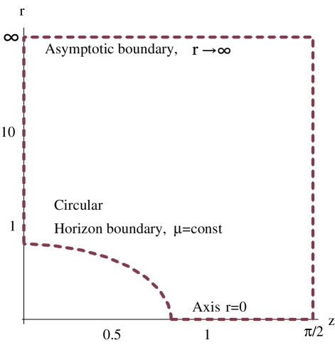
Figure 1: Schematic illustration of the boundaries we would intuitively take in $r,z$ coordinates. At least for small black holes, taking the horizon boundary to be circular would ensure the metric functions $A,B,C$ would be small and finite, as the geometry near the horizon would only be a weak distortion of 6-dimensional Schwarzschild, which we build into the metric ansatz via $A_{bg},B_{bg},C_{bg}$.

Numerically it is always convenient to have a rectangular grid. Whilst we are in principle free to use the residual conformal transformation to fix the boundaries to be wherever we wish, clearly to obtain a rectangular domain such a transformation must be singular, as one right-angle in the figure 1 should be ‘flattened’ out. However, if we find such a coordinate transformation analytically, we may separate out any singular behaviour from $A,B,C$, leaving their behaviour perfectly regular. Any conformal coordinate transformation is generated by a solution to the 2-d Laplace equation, and choosing a solution $\rho(r,z)$ to be that representing a point source in the compact 2-d space (ie. on a cylinder) we may define new coordinates $(\rho,\chi)$,

$$\rho(r,z) = \frac{1}{2}\log\left[\frac{1}{2}\left(\cosh{2\,r}-\cos{2\,z}\right)\right]$$ (6)

$$\chi(r,z) = \tan^{-1}\left[\frac{\tan z}{\tanh r}\right]$$

where $\chi$ is determined from $\rho$ by CR relations. These essentially ‘flatten’ out the horizon, and now $\chi$ is the compact coordinate which conveniently takes the range of an angular coordinate $(0,\pi/2)$ for half a period of the solution, $z=(0,L/2)=(0,\pi/2)$. We illustrate the isosurfaces of $\rho$ and $\chi$ in the $(r,z)$ plane in figure 2. Contours of constant $\rho$, for $\rho<0$, generate very similar curves in the $(r,z)$ plane to that of the horizon in figure 1. Note also that $\chi=\pi/2$ gives us both the axis of symmetry (for $\rho<0$) and the periodic boundary $z=\pi/2$ (for $\rho>0$), and $\rho=0$, $\chi=\pi/2$ is the singular point in the conformal transformation. Thus if we use these coordinates, a rectangle with $\chi=0$ to $\pi/2$ and $\rho=\rho_{0}$ to $\infty$ will, for $\rho_{0}<0$, give us similar looking boundaries to figure 1.

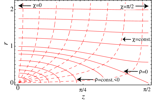
Figure 2: Illustration of isosurfaces of $\rho,\chi$ as functions of $r,z$. The schematic boundaries of figure 1 can be mapped to constant $\rho$ and $\chi$ values, making for convenient numerical implementation. For $\rho<0$, $\chi$ behaves as an angular coordinate, and $\rho$ as a radial one, whereas for large positive $\rho$, we find $\rho,\chi$ behave as $r,z$ respectively. We will take the horizon boundary at constant $\rho=\rho_{0}$, finding later that specifying $\rho_{0}$ determines the physical size of the black hole solution.

Whilst the coordinate transform is rather singular, since we have an analytic expression for it, we may remove the singular Jacobian, $J$, and now write the metric,

$$ds^{2}=-e^{2\alpha}dt^{2} + e^{2(\beta-\gamma)}J(\rho,\chi)\left(d\rho^{2}+d\chi^{2}\right)+r(\rho,\chi)^{2}e^{2\beta+\frac{4}{3}\gamma}d\Omega^{2}_{(3)}$$ (7)

$$J(\rho,\chi) = \frac{e^{2\rho}}{\sqrt{1+e^{4\rho}+2\,e^{2\rho}\cos{2\chi}}}$$

$$r(\rho,\chi) = \frac{1}{2}\cosh^{-1}\left[e^{2\rho}+\sqrt{1+e^{4\rho}+2\,e^{2\rho}\cos{2\chi}}\right]$$

where now $\alpha,\beta,\gamma$ are exactly the same functions as previously in (1), except now in terms of $\rho,\chi$.

Now consider the 6-d Schwarzschild metric (2.1). For small $\mu_{0}$, near the horizon we find $e^{2\rho}\simeq\mu^{2}=r^{2}+z^{2}$, with $\rho$ behaving as a polar radial coordinate and $\chi$ as the angular one. Since we wish to choose background functions to reproduce the Schwarzschild metric near the horizon for small black holes (ie. small $\mu_{0}$), and yet to implement the compactness requirement in $z$, a simple choice is just to substitute $e^{\rho-\rho_{0}}=\mu/\mu_{0}$ into (2.1) giving,

$$e^{A_{bg}} = \frac{1-e^{3\left(\rho_{0}-\rho\right)}}{1+e^{3\left(\rho_{0}-\rho\right)}}$$ (8)

$$e^{B_{bg}} = \left[1+e^{3\left(\rho_{0}-\rho\right)}\right]^{\frac{2}{3}}$$

$$C_{bg} = 0$$

The independence of these background functions on $\chi$ ensures they satisfy the periodicity requirements. The constant $\rho_{0}$ tells us the coordinate position of the horizon. We will shortly show that keeping the asymptotic compactification radius fixed, it is the parameter $\rho_{0}$, and thus the contour $\rho=\rho_{0}$ we take to be the horizon that we will vary to change the mass of the black hole. From the earlier figure 2 we see that $\rho_{0}$ must be negative to give a spherical topology for the horizon. The small horizon limit is now $\rho_{0}\rightarrow-\infty$. For $\rho_{0}<0$ but closer to zero, the ansatz above gives a deformed geometry from Schwarzschild too. Since we include the vanishing of the lapse in $A_{bg}$ at $\rho=\rho_{0}$ we expect the metric functions, and in particular $A$, the one associated with deformations of the lapse, to remain finite there. Far away from the horizon, ie. for $\rho\rightarrow\infty$ or alternatively $r\rightarrow\infty$, the background functions decay exponentially in $\rho$ or $r$. We stress that for finite negative $\rho_{0}$, $A,B,C=0$ is not a solution to the Einstein equations, but for very negative $\rho$, the small black hole limit, $A,B,C$ will at least be small everywhere as the horizon tends to Schwarzschild, and by the time the metric functions ‘see’ the compactification they will be vanishingly close to zero anyway. After the change in coordinates, we obtain analogous elliptic equations, $G^{t}_{~{}t},(G^{\rho}_{~{}\rho}+G^{\chi}_{~{}\chi}),G^{\theta}_{~{}\theta}$ and also CR relations for the new constraint functions $\Phi,\Psi$,

$$\Phi=\det{g_{MN}}G^{\rho}_{~{}\chi}\qquad\Psi=\frac{1}{2}\det{g_{MN}}(G^{\rho}_{~{}\rho}-G^{\chi}_{~{}\chi})$$ (9)

so that,

$$\partial_{\rho}\Phi=\partial_{\chi}\Psi\qquad\qquad\partial_{\chi}\Phi=-\partial_{\rho}\Psi$$ (10)

2.2 Boundary conditions from the elliptic equations

The 3 elliptic equations we are solving require various boundary conditions due to the regular singular or periodic behaviour at these boundaries. To satisfy the constraint equations we must impose more than just these conditions. However, let us start by considering the basic boundary conditions from the elliptic equations.

Asymptotically we want the geometry to be a product of 5-dimensional flat space with a circle, and thus we take $A,B,C\rightarrow 0$. Since we earlier fixed the range of $\chi$, this also fixes the compactification radius to be $L=\pi$. Of course we may simply globally scale these vacuum solutions to obtain any desired asymptotic radius. We find the asymptotic form required by the 3 elliptic equations,

$$A\sim\frac{a_{2}}{\rho^{2}}+O\left(\frac{1}{\rho^{3}}\right)\qquad B\sim\frac{b_{1}}{\rho}+\frac{b_{2}}{\rho^{2}}+O\left(\frac{1}{\rho^{3}}\right)\qquad C \sim \frac{b_{1}}{\rho}+\frac{c_{2}}{\rho^{2}}+O\left(\frac{1}{\rho^{3}}\right)$$ (11)

$$\mbox{with}\qquad 3\,a_{2}+9\,b_{2}-4\,c_{2}+\frac{25}{6}b_{1}^{2} = 0$$

expanding (without linearising in the metric components) in inverse powers of $\rho\sim r$. Fourier modes with $\chi$ dependence decay exponentially (since $\chi\simeq z$, for large $\rho$), as does the contribution from the background functions $\{A,B,C\}_{bg}$. Thus on our asymptotic boundary we have mixed Neumann-Dirichlet boundary conditions for the 3 metric functions.

The symmetry axis $\chi=\pi/2$ with $\rho<0$ requires that $A,B$ be even in $(\chi-\pi/2)$ (or alternatively $r$). However we also find the requirement that $C=0$ as there is a regular singular behaviour due to the form of the coordinate system. We might be confused that there is no Neumann condition on $C$ but we see later this emerges from the constraints.

We require that the metric functions $A,B,C$ be finite at the horizon $\rho=\rho_{0}$. With the form of background functions $\{A,B,C\}_{bg}$ we then find that the elliptic equations are consistent provided that,

$$A_{,\rho}\mid_{\rho=\rho_{0}} = 0$$ (12)

$$B_{,\rho}+\frac{2}{3}C_{,\rho}\mid_{\rho=\rho_{0}} = 1-\frac{r_{,\rho}}{r}\mid_{\rho=\rho_{0}}$$

with $r(\rho,\chi)$ as given earlier in equation (7).

Finally, the elliptic equations at the remaining periodic boundaries at $\chi=0$ and $\chi=\pi/2$ with $\rho>0$ simply imply Neumann conditions on the metric functions $A,B,C$.

2.3 Boundary conditions from the constraints

The constraint equations also impose conditions on the metric. We have seen that assuming we can satisfy the elliptic equations for given boundary data, the two constraints obey CR relations. Thus we do not need to enforce both constraints on all the boundaries, which naively would over-determine the elliptic equations. Firstly we consider the extra conditions the constraints impose, and then discuss how best to implement them to ensure a consistent solution of the CR problem, without over determining the elliptic data.

On the symmetry axis and periodic boundaries we have already specified 3 conditions, one for each metric function, and consequently treating this as a boundary value problem, we do not wish to impose any more. On the $\chi=0$ periodic boundary $G^{\rho}_{~{}\chi}$ vanishes by symmetry, and consequently so does the corresponding weighted constraint $\Phi$, and the remaining constraint $(G^{\rho}_{~{}\rho}-G^{\chi}_{~{}\chi})$ is guaranteed to be even. A similar situation occurs on the $\chi=\pi/2$ boundary for $\rho>0$ which represents the other periodic boundary. Indeed these periodic boundaries are fictitious in the sense that we can consider the problem on the unwrapped covering space where these boundaries are ‘removed’, and thus we should not need to impose any constraints here.

For $\chi=\pi/2$, but now with $\rho<0$ we have the symmetry axis. Again this is in principle a ‘fictitious’ boundary, but we must impose $C=0$ here for the elliptic equations, and it is hard to see how this would lift to a covering space with ‘no’ boundary. Thus we examine the situation at the axis in more detail. Using the boundary conditions from the elliptic equations, and assuming the metric components are regular, $G^{\rho}_{~{}\chi}$ vanishes there, but $(G^{\rho}_{~{}\rho}-G^{\chi}_{~{}\chi})$ does not unless the normal gradient of $C$ vanishes. However, since the measure $\det{g_{MN}}$ vanishes near this axis, both $\Phi$ and $\Psi$ are zero, and so from the point of view of solving the CR constraint equations we need do no more here. As discussed in the original implementation of this method [18], this resolves the paradox that $C=0$ and $C$ has a Neumann boundary condition, despite us solving $C$ using a boundary value formulation. Whilst we only impose $C=0$ to be compatible with the elliptic equation behaviour, if we consistently provide data on the other boundaries to ensure the weighted constraints vanish everywhere, then this Neumann condition follows automatically, and does not need to be explicitly imposed at the symmetry axis.

Now let us consider the remaining boundaries, the horizon and asymptotic boundary. At the horizon we only have 2 conditions from the elliptic equations and require another to specify elliptic data. Firstly at the horizon we find that the $G^{\rho}_{~{}\chi}$ constraint implies the horizon temperature is a constant,

$$\left(A-B+C\right)_{,\chi}\mid_{\rho=\rho_{0}}=\frac{1}{2}\frac{J_{,\chi}}{J}\mid_{\rho=\rho_{0}}$$ (13)

and the remaining constraint $(G^{\rho}_{~{}\rho}-G^{\chi}_{~{}\chi})$ requires,

$$\left(A-B+C\right)_{,\rho}\mid_{\rho=\rho_{0}}=\frac{1}{2}\frac{J_{,\rho}}{J}\mid_{\rho=\rho_{0}}-1$$ (14)

Lastly, asymptotically at large $\rho$ (or equivalently $r$) due to the exponential decay of $\chi$ (or equivalently $z$) dependence the $G^{\rho}_{~{}\chi}$ constraint goes exponentially to zero, and so the weighted constraint $\Phi$ is guaranteed to go to zero, even though $\det{g_{MN}}\sim\rho^{3}$. Due to this power law growth of the measure $\det{g_{MN}}$, it is less obvious the $(G^{\rho}_{~{}\rho}-G^{\chi}_{~{}\chi})$ constraint weighted as $\Psi$ goes to zero, as $(G^{\rho}_{~{}\rho}-G^{\chi}_{~{}\chi})$ (unlike $G^{\rho}_{~{}\chi}$) depends on the homogeneous components of the metric, which only decay as a power law. However, the behaviour of the homogeneous component implied by the elliptic equations in (11) does also ensure that $\Psi=0$ asymptotically.

Now we must decide how to specify data for the elliptic equations (ie. one condition for each metric function on each portion of boundary), but also satisfy the constraint problem. With the conditions already required by the elliptic equations, we have sufficient data and $\Phi=0$ on all boundaries except the horizon. The second weighted constraint $\Psi=0$ is satisfied only asymptotically. At the horizon neither constraint is satisfied, and we require one more condition for a linear combination of $A,B,C$ to make up the elliptic data as we so far only have (12).

We could impose the constant horizon temperature condition and thus set $\Phi$ to zero on the horizon. As we have seen $\Phi$ is zero on all the other boundaries, and from the CR relations it obeys a Laplace equation, so this would uniquely set it to zero everywhere. $\Psi$ would then be zero following from the CR relations and the fact it vanishes asymptotically.

However it is numerically more stable to impose the $(G^{\rho}_{~{}\rho}-G^{\chi}_{~{}\chi})$ constraint, and hence $\Psi=0$ at the horizon instead. The $(G^{\rho}_{~{}\rho}-G^{\chi}_{~{}\chi})$ constraint is a typical elliptic boundary condition, whereas imposing the constant horizon temperature $G^{\rho}_{~{}\chi}$ constraint involves ‘less local’ tangential derivatives on the horizon. Now we have sufficient data to impose both constraints globally via the CR problem. Since at the horizon $\Psi=0$, $\Phi$ has a Neumann condition there, and is zero on all other boundaries, and hence will be zero everywhere as it obeys a Laplace equation. The CR relations then imply that $\Psi$ is constant, and must be zero as it was imposed to be zero on the horizon and is also true asymptotically.

2.4 How $\rho_{0}$ specifies the size of the black hole

Fixing $A,B,C\rightarrow 0$ asymptotically, and thus the asymptotic compactification radius to be $L=\pi$, there must be one constant entering the boundary data that specifies the size, or mass of the black hole. Intuitively one would imagine this to be $\rho_{0}$ as this certainly enters into the boundary data at the horizon, in equations (12) and (14).

To confirm this, we must demonstrate that $\rho_{0}$ is a physical quantity, and not simply a coordinate artifact. Thus we must show there is no residual coordinate transformation (ie. conformal transformation on $\rho,\chi$) that preserves the rectangular boundaries, and conditions on these boundaries, and the asymptotic radius of compactification, but changes the effective $\rho_{0}$ in the new coordinates. If this were the case, $\rho_{0}$ would not correspond to a physical parameter, and therefore could not specify the size of the black hole, which certainly is a physical parameter.

Let us suppose we have a black hole solution with a particular $\rho_{0}$. Now let us construct the most general coordinate transformation that simply preserves the rectangular boundaries. We construct new coordinates $\rho\rightarrow\tilde{\rho}=\tilde{\rho}(\rho,\chi)$, $\chi\rightarrow\tilde{\chi}=\tilde{\chi}(\rho,\chi)$, and then must solve a CR problem to build the conformal coordinate transformation. Let us do this by specifying data for the Laplace equation that determines $\tilde{\chi}$. For the boundaries to remain rectangular, we must specify constant $\tilde{\chi}=\tilde{\chi}_{0}$ on the $\chi=0$ boundary and constant $\tilde{\chi}=\tilde{\chi}_{\pi/2}$ on the $\chi=\pi/2$ boundary. At the horizon, we must specify a Neumann condition on $\tilde{\chi}$ and then the CR equations guarantee $\tilde{\rho}$ is constant there. Regular asymptotics then give the unique solution,

$$\tilde{\chi}=\tilde{\chi}_{0}+\left(\tilde{\chi}_{\pi/2}-\tilde{\chi}_{0}\right)\frac{\chi}{\pi/2}$$ (15)

This solution now completely determines $\tilde{\rho}$ up to a further constant of integration.

Now that we have the general transform preserving the rectangular boundaries, let us further restrict it by making it preserve our boundary conditions. Firstly, since $\tilde{\chi}_{0}$ does not enter into any equation or boundary condition, we may freely set this to zero. Secondly, since we have selected $A,B,C\rightarrow 0$ asymptotically, we require $\tilde{\chi}=\pi/2$ on the $\chi=\pi/2$ boundary if we are not to change the compactification radius $L=\pi$. Thus now, $\tilde{\chi}=\chi$. This implies from the CR relations,

$$\tilde{\rho}=\delta\rho_{0}+\rho$$ (16)

where $\delta\rho_{0}$ is a constant of integration.

However there is a subtle point. Whilst $\rho_{0}$ only enters the boundary conditions explicitly at the horizon, the boundaries conditions change on the $\chi=\pi/2$ axis for $\rho>0$ (where $C$ has a Neumann condition imposed) to $\rho<0$ (where $C=0$ is imposed). Since we have fixed this transition of boundary conditions to occur at $\rho=0$, in the new coordinates this will occur at $\tilde{\rho}_{0}=\delta\rho_{0}$. Hence the transformed solution will not satisfy the boundary conditions in the new coordinates where this transition now occurs at $\tilde{\rho}=0$. Thus, due to our fixing the transition from symmetry axis to periodic boundary at $\rho=0$, there are no residual coordinate transformations mapping solutions with horizon position $\rho_{0}$ to a transformed solution, solving the boundary conditions but with a different horizon position $\tilde{\rho}_{0}$ in the new coordinates. Therefore $\rho_{0}$ does indeed specify the physical size of the black hole.

2.5 Thermodynamic quantities

We will compute the temperature $\mathcal{T}$ and entropy $\mathcal{S}$ of the black hole solutions, and these are given as,

$${\cal T} = \frac{1}{2\pi}\frac{3e^{A-B+C}}{2^{8/3}\sqrt{J}}\mid_{\rho=\rho_{0}}$$ (17)

$${\cal S} = \frac{1}{4}\left[2e^{4R_{S}}\int d\Omega_{3}\int^{\pi/2}_{0}d\chi\sqrt{J}r^{3}e^{4R+C}\right]_{\rho=\rho_{0}}$$ (19)

The mass may be computed by two independent methods. Firstly we may determine the mass from the asymptotics of the metric, as,

$$M=\frac{\pi^{2}L}{4}\left(-3a_{2}-b_{2}+c_{2}\right),$$ (20)

using the expansions (11)[54]. Secondly the mass may be determined by integration from the First Law, using $dM/d\rho_{0}=\mathcal{T}(\rho_{0})d\mathcal{S}/d\rho_{0}$ (which applies for fixed asymptotic compactification radius - see below) along the branch of solutions, and taking $M=0$ for $\rho_{0}\rightarrow-\infty$ to define the integration constant. Later (figure 9) we will see very good agreement between these two values. This is a good indication that the elliptic equations are well satisfied globally and the boundary conditions are imposed correctly. An important point is that the First Law does not test whether the constraint equations $G^{r}_{~{}z},(G^{r}_{~{}r}-G^{z}_{~{}z})$ are satisfied, and we elaborate on this point in Appendix C. Since we completely relax the elliptic equations, it is then not terribly surprising that the First Law holds very well. What is absolutely essential is that the constraints are also checked, to ensure they are well satisfied. They indeed are, and these tests are outlined in Appendix B.

Since the black hole geometries are compactified, the mass is not the only asymptotic charge. This feature, shared more generally by branes was originally discussed in [55], and more recently in relation to the black hole/black string problem in [26, 27, 28]. It is easy to see there must be another charge. As the geometry becomes homogeneous at large distances from the symmetry axis it can be dimensionally reduced to Einstein-dilaton-Maxwell theory. For our regular static solutions the Maxwell vector can always be gauged away, but we are left with gravity and the dilaton scalar, indicating we should consider both an asymptotic mass, but also a scalar charge.

From a purely 6-dimensional point of view, the second charge can be thought of as a binding energy per unit mass, $n$, resulting in a modified First Law,

$$dM=T\,dS+n\,M\,\frac{dL}{L}$$ (21)

with the new term representing work done when varying the asymptotic size of the extra dimension. In our solutions, fixing $L$ we reproduce the usual form of the First Law for black holes. However, we may determine $n$ from the asymptotics of the metric, or from the Smarr relation,

$$TS=\frac{3-n}{4}M$$ (22)

again discussed in [55], and given explicitly for the problem at hand in [26, 27], where $n$ was calculated from the asymptotics to be,

$$n=\frac{a_{2}+3\,b_{2}-3\,c_{2}}{3\,a_{2}+b_{2}-c_{2}}$$ (23)

As emphasised in [27] we may use the Smarr formula as a check of our numerics. This is very similar to the First Law check discussed above, which only involves the mass, whereas Smarr’s law involves both $M$ and $n$. It is important to note that for the same reasons the First Law does not probe the constraint equations, the Smarr formula also does not. Thus again it is no replacement for the checking of constraint equation violations we perform in Appendix B.

2.6 Behaviour of the method

Following the above method, we may construct a unique numerical solution for each value of $\rho_{0}$. The elliptic equations can be solved very stably, once the coordinate induced instability at the axis is dealt with (see Appendix A). Since we have designed the coordinates and method to have $A,B,C\rightarrow 0$ in the small black hole limit $\rho_{0}\rightarrow-\infty$, the method behaves well in this limit. As the black hole becomes larger, so $\rho_{0}$ is finite and negative, $A,B,C$ deviate away from zero, although remain regular as we expect. Topology of the $\rho$ coordinate dictates $\rho_{0}=0$ is the largest black hole that could exist. Using reasonable resolutions (up to $\sim$ 140*420), we were able to find solutions with a maximum $\rho_{0}\simeq-0.18$, yielding a black hole horizon with typical radius comparable to the asymptotic compactification radius. As an example we show the metric functions $A,B,C$ for $\rho_{0}=-0.28$ in figure 3. Note that the magnitude of $C$ is much less than that of $A,B$, and this is increasingly true the smaller the black hole. Hence the spatial sections are approximately conformally flat.

The larger the black hole is, the larger the gradients in the metric functions, and for a fixed resolution the method no longer converges past a certain black hole size. Going to a higher resolution we find the problem is removed, and the size can be further increased, but obviously the problem then re-occurs at a new larger size. The key area where we lack resolution is near the symmetry axis. For the large black holes, with $\rho_{0}$ closer to zero, there become fewer and fewer points there. With the maximum size we could find, $\rho_{0}=-0.18$, so the coordinate distance of the symmetry axis is $0.18$, compared to the coordinate distance along the horizon which is $\pi/2\sim 1.6$, and hence with our simple discretization scheme (see Appendix A for details) the axis is allocated far fewer points. The closer $\rho_{0}$ gets to zero, the more acute this problem. Thus in our simple numerical implementation, we are limited by resolution, and hence computation time. We present results in this paper using modest resources and simple relaxation algorithms. It is likely that with improvements in both areas one can achieve far improved data. For example, adaptive grid methods may circumvent the lack of resolution near the symmetry axis, but it is a serious challenge to implement these and maintain a stable relaxation agorithm. However, already with our simple implementation it is possible to derive interesting physical results as we shall see.

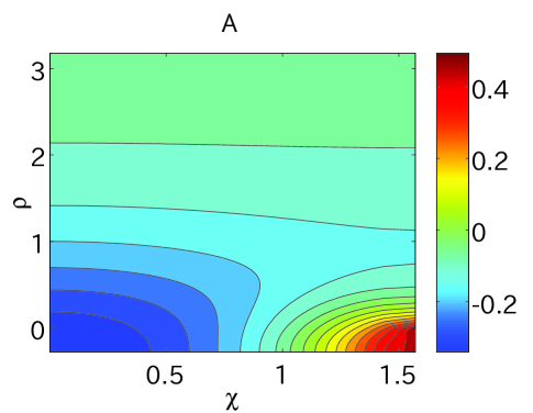
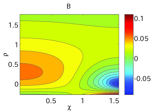
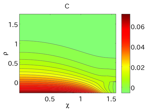
Figure 3: Plots of the metric functions $A,B,C$ for a black hole solution with $\rho_{0}=-0.28$. This is quite near to the maximal size ($\rho_{0}=-0.18$) we were able to construct before we become limited by gradients and lattice resolution near the symmetry axis at $\chi=\pi/2$ for $\rho<0$. Already this black hole solution has equal horizon volume and mass to the most non-uniform strings compactified on the same asymptotic radius. Whilst the lattice is large, being $140*420$ in $\chi,\rho$, since $\rho_{0}$ is very close to zero the number of points along the symmetry axis is only around $\sim 20$. This is still enough to see good behaviour in the metric functions. Note that $B,C$ are much less than $A$ in magnitude. The maximum $\rho$ for the lattice is $\sim 5$, and not all the domain is shown as the functions simply go smoothly to zero at large $\rho$.

3 Results

The questions we wish to address are whether there is an upper mass limit for these solutions, and whether the geometry is compatible with continuation to the non-uniform string branch. Whilst $\rho_{0}=0$ is the largest black hole due to the topology of the $(\rho,\chi)$ coordinate system, obviously the metric functions $A,B,C$ may diverge in this limit, and consequently so might the horizon volume and mass, and thus a priori we have no reason to assume such an upper mass limit will exist. On physical grounds one could argue that a black hole would not be able to ‘fit’ into the compact extra dimension, but we stress that in the unstabilised pure Kaluza-Klein theory it is only the asymptotic radius we have fixed for the branch of solutions, and there is nothing to prevent the geometry along the axis and horizon from decompactifying as the black hole becomes larger.

3.1 Horizon geometry

In order to approach these questions we embed the spatial horizon geometry into 5-dimensional Euclidean space,

$$ds^{2}=dX^{2}+dY^{2}+Y^{2}d\Omega^{2}_{(3)}$$ (24)

and matching our geometry at $\rho=\rho_{0}$ implies that,

$$Y(\chi) = r\,e^{\beta+\frac{2}{3}\gamma}\mid_{\rho=\rho_{0}}$$ (25)

$$X(\chi) = \int_{0}^{\chi}d\chi^{\prime}\sqrt{\left[J(\chi^{\prime})\,e^{2(\beta-\gamma)(\chi^{\prime})}-\rho_{,\chi^{\prime}}^{2}\right]}_{\rho=\rho_{0}}$$

and we interpolate the numerical data to perform the integral. Clearly for small black holes we expect a spherical horizon, and for larger black hole we expect deformation. We find excellent agreement with the horizon being a prolate ellipsoid for all our solutions up to the maximum size available $\rho_{0}=-0.18$. In figure 4 we plot a moderate and a large black hole to demonstrate the accuracy of the ellipsoid fit. We plot the positions of the actual lattice points in the embedding coordinates $X,Y$ for our highest resolution, and against these we plot the fitting ellipse, and note that all the points fall consistently on the fit curve. Thus from now on it is easier for us to characterise the geometry using the major (polar) and minor (equatorial) axis radii, which we term $R_{polar},R_{eq}$. Then using this elliptical fit we plot the ellipse radii and ellipticity,

$$\epsilon=\frac{R_{eq}}{R_{polar}}$$ (26)

against $\rho_{0}$ for all our solutions in figure 5. We see that for the largest black holes the ellipticity decreases to only $\sim 0.87$, even though the ellipsoid radius $R_{polar}$ increases to $\sim 1.5$, which is approximately the size of the asymptotic compactification half-period $L/2=\pi/2$. Thus it is clear from the prolateness and lack of deformation that the geometry around the symmetry axis is decompactifying.

We now wish to characterise this decompactification. In figure 6 we plot a selection of black hole embeddings, now including the embedding of the symmetry axis to show its proper length. Note that we only show half of the full period, and thus reflecting the horizon and axis about $X=0$ generates the full compact period. The asymptotic compactification radius for half the period is $L/2=\pi/2$ here. We term the length of the axis for half the period, $L_{axis}$, and it is given as,

$$L_{axis}=\int_{\rho_{0}}^{0}d\rho Je^{\beta-\gamma}\mid_{\chi=\pi/2}$$ (27)

We see $L_{axis}$ decreases in these figures for larger black holes, but the horizon radii increase faster, resulting in an overall decompactification. In figure 7 we show the maximum value of the embedding coordinate $X$ to contain half a period of both the horizon and the symmetry axis,

$$X_{max}=X(\pi/2)+L_{axis}$$ (28)

which is essentially the same as $(R_{polar}+L_{axis})$ since the ellipse is such a good fit to the horizon geometry. We take this quantity to be the physically relevant (and coordinate invariant) measure of the compactification length near the axis.

These plots clearly show the axis decompactifying. Since we are only able to ‘grow’ black holes to $\rho_{0}=-0.18$, it is unclear whether; i) there exists a maximal mass black hole, or ii) whether the decompactification continues in such a way that arbitrarily large black holes may exist, eg. with $L_{axis}\rightarrow 0$ or a constant in the limit of infinite mass. If there were a maximum mass, it seems likely from the figures that $\rho_{0}$ can still be increased some way more before we would expect to reach it.

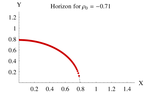
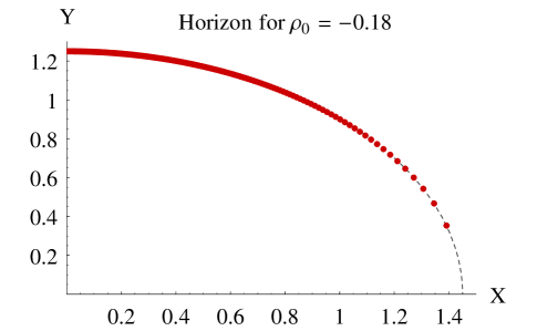
Figure 4: Embedding of horizons into Euclidean space for a moderate black hole on the left, with $\rho_{0}=-0.71$, and the maximal black hole to the right with $\rho=-0.18$. Whilst we interpolate the numerical functions to determine the embedding, we plot here the actual positions of the lattice points for our highest resolution to give an indication of how the resolution varies with position on the horizon. For all the solutions, we may fit a prolate ellipsoid to the horizon, the dashed line, and in all cases find perfect agreement.

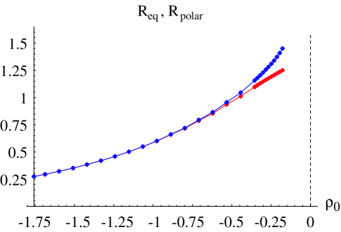
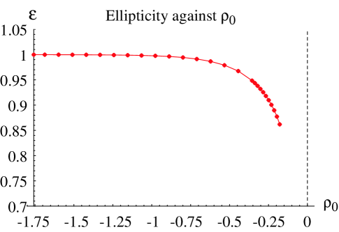
Figure 5: On the left we plot the equatorial (red) and polar (blue) radii of the ellipses fitted to the horizon embeddings, against the parameter $\rho_{0}$ specifying the size of the black hole. It is unclear what happens in the limit $\rho_{0}\rightarrow 0$ where the $\rho$ coordinate changes topology. It would be very interesting to know if $R_{eq},R_{polar}$ remain finite or not, and thus whether there is a maximum mass black hole or not. Since the geometry near the axis and horizon decompactifies, even though the largest black holes found have comparable radii to the corresponding asymptotic half period distance $L/2=\pi/2$, the horizons are still quite spherical. We plot the ratio of the radii in the right hand diagram. Again it is unclear what will occur in the limit $\rho_{0}\rightarrow 0$.

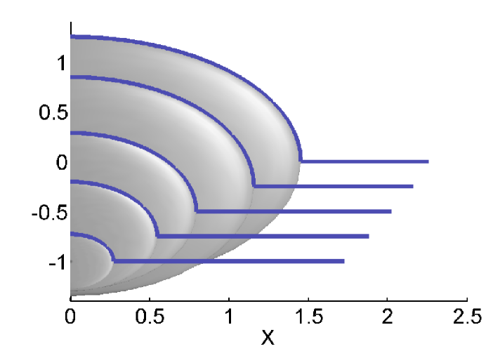
Figure 6: We show both the embedding of the horizon, and also the symmetry axis for various solutions ranging up to the largest black hole found. These embeddings are for half a period, and should be reflected about $X=0$ to obtain the full geometry. The asymptotic radius of this half period is $L/2=\pi/2$. We clearly see that the total space taken up by the solutions in the embedding $X$ coordinate grows as the black hole increases in size, despite the symmetry axis decreasing in length, indicating the overall geometry near the horizon and axis decompactifies. We also see that even the largest black hole still appears to have considerable ‘room’ to increase its size still further.

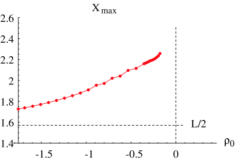
Figure 7: Plot showing $X_{max}$, the ‘length’ taken up by half the horizon and symmetry axis when embedding into Euclidean space. This quantity offers a physical and coordinate invariant measure of the radius of compactification near the horizon. We see as the black hole grows, with increasing $\rho_{0}$, the axis decompactifies considerably. Again, it is unclear what happens in the $\rho_{0}\rightarrow 0$ limit.

3.2 Comparison with non-uniform strings

We now compare these geometries with those of the critical uniform string ($\lambda=0$), and the most non-uniform strings ($\lambda\simeq 4$) found in [12], rescaling the asymptotic radius appropriately, and defining $\lambda$ as in that paper,

$$\lambda=\frac{1}{2}\left(\frac{R_{max}}{R_{min}}-1\right)$$ (29)

where $R_{max,min}$ are the maximum and minimum horizon radii respectively. Whilst $\lambda=3.9$ was the most non-uniform string found there, the geometry and also thermodynamic quantities $M,\mathcal{T},\mathcal{S}$ appear to asymptote for large $\lambda$ (see also [29]) and thus the $\lambda\rightarrow\infty$ values are expected to be very similar to those at $\lambda\simeq 4$, probably only differing by a few percent. Strong evidence for this comes from the realization that a conical geometry forms at large $\lambda$, as tested in [30]. Once $\lambda$ is relatively large, say $\lambda\sim 2$, only the geometry near the string ‘waist’ appears to change with increasing $\lambda$ as the cone forms. With the rescaling so that the asymptotic radius for one period of the solution is $L=\pi$, we find the following values,

$$\mbox{Critical string}\qquad R_{max,\lambda=0} = 0.64$$ (30)

$$X_{max,\lambda=0} = \frac{\pi}{2}$$

$$M_{\lambda=0} = 1.47$$

$${\cal T}_{\lambda=0} = 0.250$$

$${\cal S}_{\lambda=0} = 3.99$$

$$\mbox{Highly non-uniform string}\qquad R_{max,\lambda=3.9} = 1.11$$

$$X_{max,\lambda=3.9} = 1.91$$

$$M_{\lambda=3.9} = 3.38$$

$${\cal T}_{\lambda=3.9} = 0.184$$

$${\cal S}_{\lambda=3.9} = 12.94$$

Here $R_{max,\lambda}$ is the maximal radius of the horizon, and $X_{max,\lambda}$ is again the maximum value of $X$ when embedding half a period of the strings into Euclidean space, using the metric (24) as for the black holes, and taking $X=0$ at the maximal radius of the horizon, so $X=X_{max}$ at the ‘waist’, the minimum radius. Now, there is no exposed symmetry axis, so $X_{max}$ is just the change in $X$ when traversing the horizon for a half period. As noted in [29] the proper distance (which is not equal to the embedding coordinate $X$) along the horizon increases with $\lambda$ indicating the geometry decompactifies there.

The key observation of this paper is now evident from the previous plots of the embedded black hole geometry. Already for $\rho_{0}\simeq-0.35$ we see the black hole equatorial radius $R_{eq}$ is equal to $R_{max}$ for the highly non-uniform $\lambda=3.9$ non-uniform string, which as stated above we take to be approximately equal to $R_{max}$ in the limit $\lambda=\infty$. And as $\rho_{0}$ increases past this point, the black holes continue to become larger in radius. In addition we also see from $X_{max}$ that the geometry along the axis has decompactified as much as that of the very non-uniform strings for even quite small black holes with $\rho_{0}\simeq-1.0$, and again the trend seems to continue for increasing $\rho_{0}$ past this point. The implication is clear, that it seems difficult to imagine the black hole solutions making a transition at $\rho_{0}=0$ via a cone geometry to the most non-uniform strings, when they simply become ‘bigger’ than the most non-uniform strings already for $\rho_{0}\simeq-0.35$. We may gain more insight into this result in figure 8 by plotting the embedding of the $\lambda=3.9$ non-uniform string, and the largest black hole relaxed ($\rho_{0}=-0.18$) into Euclidean space, including the symmetry axis of the black hole. Again we note that with increasing $\lambda$ past 3.9 we only expect the geometry in the cone region to change, and thus the geometry of the $\lambda=3.9$ string should be very close to that of the limiting string at $\lambda=\infty$ (see [29] for curves of $R_{max}$ against $\lambda$).

Whilst we earlier claimed that resolution becomes limited near the horizon and axis for the large black holes, we find that the values of $R_{eq},R_{polar}$ only vary by $\sim 1\%$ when doubling the resolution from $70*210$ to our highest resolution $140*420$ for the solution with $\rho_{0}\simeq-0.35$ that parallels the most non-uniform string horizon size. The length along the axis $L_{axis}$ varies only a little more, around $\sim 3\%$. Thus while decreasing axis resolution with increasing black hole size limits the ability of the algorithm to converge, the resolution is still high enough for the accuracy of our large black hole solutions to be high. For further comparison of quantities measured at different resolutions, see figure 9 and the Appendix A.

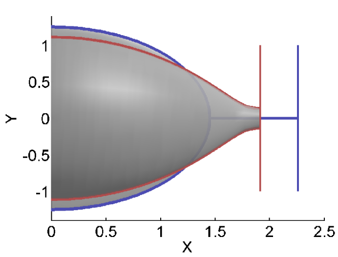
Figure 8: An illustration of the intrinsic geometries of the maximum sized black hole found ($\rho_{0}=-0.18$) compared to a highly non-uniform string ($\lambda=3.9$) whose geometry is expected to be very close to the limiting $\lambda=\infty$ solution, with a conical geometry near the waist of the horizon. Only half a period of the solutions is shown, and for the full geometry one should reflect about $X=0$. Both are taken to have an asymptotic compactification half period $L/2=\pi/2$. We see immediately that the black hole is simply ‘bigger’ in all aspects. It has larger equatorial radius, and including the exposed symmetry axis, it takes up more ‘room’ in the $X$ direction - ie. it has decompactified more. Indeed we also find it has a higher mass, and lower temperature. Furthermore, it looks very much as if we can increase the black hole size further still. The implication is that the $\lambda=\infty$ string solution presumably cannot be connected (through a conical topology change) to this branch of black hole solutions.

3.3 Thermodynamics

Now we turn to the thermodynamic quantities to see whether our comparison of the black hole/string horizon intrinsic geometry is parallelled in these independent observables. We might now reasonably expect the mass of the black holes to become greater than that of the most non-uniform strings, and the horizon temperature to become less. In figure 9 we plot the temperature, $\mathcal{T}$, and mass $M$ of the black hole solutions, now against the horizon entropy $\mathcal{S}$. The mass is computed in two ways, firstly asymptotically from the metric [see equation (20)], and secondly by integration from the First Law. We clearly see very good agreement for these as expected. As discussed earlier in section 2.5, this is a good test of the elliptic equations, but does not test the constraints which are the really important quantities to check for this elliptic method, as they are not imposed directly. These constraints are tested explicitly in Appendix B.

On these plots we also show the same quantities for the non-uniform string branch up to $\lambda=3.9$. Again we emphasise that the $\lambda=3.9$ point probably lies very close to the $\lambda=\infty$ point on this diagram. Our expectations are confirmed, with the temperature becoming lower, and the mass becoming higher than the most non-uniform strings already by $\rho_{0}\simeq-0.30$, and the trend continuing for larger $\rho_{0}$, again reflecting the fact that the black holes become ‘bigger’ than the non-uniform strings. We also plot the behaviour of a 6-dimensional Schwarzschild solution, and find that since the axis is decompactifying, and as a consequence the black hole horizon geometry is only slowly deforming from being a sphere, the black holes closely reproduce this Schwarzschild behaviour.

There is one further point we may observe from these plots. The non-uniform branch presumably terminates at $\lambda=\infty$, very close to the $\lambda=3.9$ solutions plotted, so the whole non-uniform branch of solutions $\lambda=0$ to $\infty$ then appears to lie very close to the black hole curves both in $\mathcal{M}$ and $\mathcal{T}$ against $\mathcal{S}$. Since the branches do not appear to connect, we can think of no particular reason why this should be so, and presumably it is just an interesting coincidence.

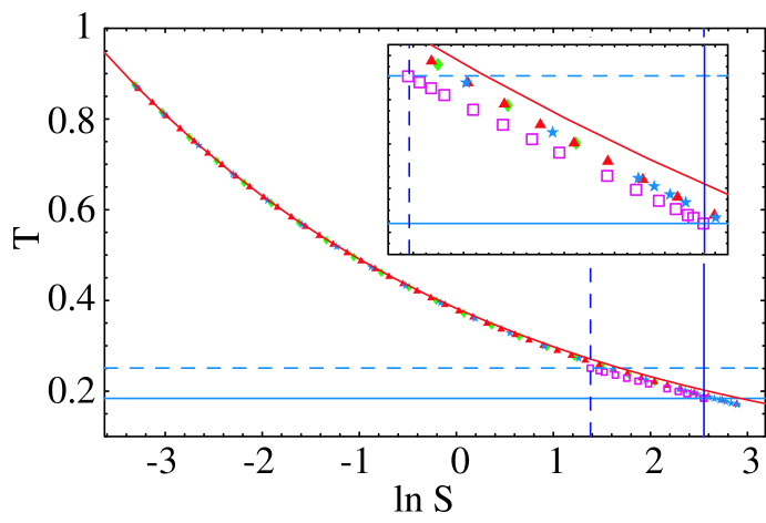
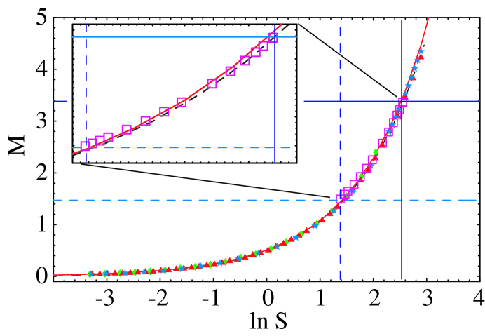
Figure 9: Plot showing black hole temperature $\mathcal{T}$ and mass $M$ against entropy $\mathcal{S}$ calculated by eqns. (19) and (20). Three resolutions for the black holes are used, $36*106$ in green, $70*210$ in red, $140*420$ in blue, and excellent consistency is found. In the figure for the mass, the dashed black line line gives the mass computed by integration from the First Law, showing excellent agreement with the asymptotically measured mass. The solid red lines give the behaviour of a 6-dimensional Schwarzschild solution, and for these black holes, despite their size becoming equivalent to the compactification radius, we see little deviation from this. We also show the same quantities plotted for the non-uniform strings as pink open squares. The dashed and solid straight lines show the limiting values for $\lambda=0$, and $\lambda\rightarrow\infty$. We include magnifications of the region where the non-uniform strings exist. Interestingly the non-uniform values lie very close to the black hole curves, although this appears simply to be coincidence.

Finally we turn to the last (and truly higher dimensional) thermodynamic quantity, the binding energy $n$ of our solutions. This turns out to be very small, and thus prone to numerical error. Referring back to (23) we recall $n$ to be given by a ratio of asymptotic quantities, with numerator $3\,b_{2}-3\,c_{2}+a_{2}$. In figure 10 we plot the magnitudes of both a term in the numerator, and the numerator itself, and demonstrate that the numerator is relatively very small, $\sim 10\%$ of the terms making it up, indicating cancellations occur between the terms. This is a problem numerically since the asymptotic quantities $a_{2},b_{2},c_{2}$ are already difficult to measure, and thus a quantities depending on detailed cancellations between them certainly should not be trusted. A further caveat is that for small black holes both the numerator and denominator are small, and their ratio is consequently extremely unreliable. Computing $n$ from the asymptotics we find its value to be less than $\sim 0.1$ for these solutions, but the errors appear large, and we stress simply that it is small, and we do not feel we can give its value with certainty here. We may reassure ourselves that whilst $n$ is ‘noisy’ in the numerical error, this is simply because $n$ is close to vanishing, and Smarr’s law is extremely well satisfied. Also in figure 10 we plot the two sides of the Smarr relation (22), $TS$ and $(3-n)M/4$, against $\rho_{0}$. In addition, we also plot $3M/4$, ie. setting $n=0$, on the same plot, which lies so close to the curve with the actual measured $n$, that it is clear $n$ is quantitatively small, and furthermore we cannot currently expect to measure it with any accuracy as argued above. Much higher precision would be required for this, and thus we leave determining the actual (small) values of $n$ for future work.

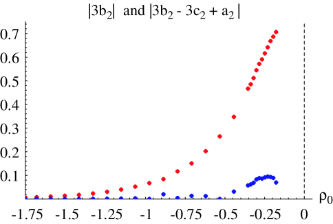
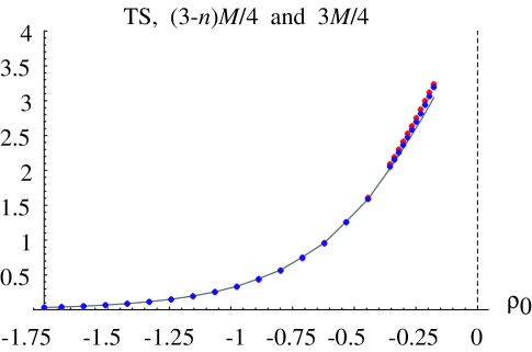
Figure 10: Left; A plot of the magnitude of a term in the numerator of ‘n’, the binding energy, and the magnitude of the numerator itself. We see this numerator is $\sim 10\%$ of the value of one of its constituent terms, and thus detailed cancellations occur, and the value of ‘n’ is very small. Since the asymptotic quantities $a_{2},b_{2},c_{2}$ are already difficult to compute accurately, we should not trust a numerical quantity that depends on detailed differences of these, and thus is very small in comparison. Right; A plot of the left- ($TS$ as a solid black line) and right-hand ($(3-n)M/4)$ as blue points) sides of Smarr’s formula, confirming that whilst $n$ is very hard to determine accurately, Smarr’s formula is very well satisfied by our data. To confirm that ‘n’ is indeed extremely small, we show the right-hand side computed with $n=0$, ie. $3M/4$ as red points, which gives a slightly worse fit, but only marginally.

4 Discussion and Outlook

We have shown that static black holes in pure 6-dimensional gravity compactified on a circle, ie. Kaluza-Klein black holes, may be found using elliptic numerical methods. As expected, for fixed asymptotic compactification radius, the small black holes behave as 6-dimensional Schwarzschild solutions. As they grow the geometry on the axis decompactifies relative to the fixed asymptotic radius, and the horizon deforms to a prolate ellipsoid. Since we are limited by numerical resolution, we are currently unable to probe whether the axis decompactifies indefinitely, and consequently black holes of any mass can be found, or whether instead there is an upper mass limit for the black holes. This is clearly an interesting issue to resolve in future work.

The most interesting result we find is that whilst we are only able to compute black holes whose radii become approximately equal to the asymptotic compactification radius, these are already sufficiently large that they are simply ‘bigger’ than the most non-uniform string solutions constructed in [12], both in terms of horizon volume and mass. For the largest black hole solutions we found the horizons are still quite spherical since the axis geometry decompactifies, making ‘room’ for the horizon. It therefore appears that they should be able to further increase in size and mass, past the point where we are currently able to construct them, before any possible upper mass limit would be reached. Given these results, it therefore seems rather unlikely that this black hole branch of solutions can merge with the non-uniform strings via a conical geometry developing at the polar regions of the horizon, as suggested by Kol [23]. This is despite the fact that we have excellent numerical evidence that the highly non-uniform strings do indeed exhibit the required conical geometry at their waist, which previously lent weight to this conjecture [30].

This is then very interesting geometrically, and raises the obvious question of whether the static non-uniform string solutions can be continued through the $\lambda\rightarrow\infty$ solution with its conical waist to a new branch of black hole solutions. Obviously while these would have horizons that do not wrap the extra coordinate, they would be distinct solutions from the ones we construct here, and at low mass (if they have a low mass limit) would presumably not look like the 6-dimensional Schwarzschild solution. Similarly, if the black hole branch we partially construct here does turn out to have an upper mass limit, can this branch of solutions be continued through to a new string solution, distinct from that connected to the Gregory-Laflamme critical uniform string? We refrain from speculating on these questions (see the recent [28] for an interesting discussion of a variety of possibilities), deferring these issues until improved numerics can be performed that confirm the current results, and can extend the range of these elliptic methods so these questions may be tackled directly. We do make one further general comment here. As we have seen comparing the current work here with the previous work constructing the non-uniform string solutions [12], the fact that the axis of symmetry is exposed for the black hole solutions completely changes the boundary conditions imposed on the problem. Thus, without proof, it would be dangerous to assume that continuation of a branch of solutions through topology change at a conical region must always be possible.

Whilst our computations were performed in 6-dimensions, in order to make contact with previous work constructing the non-uniform strings, it would be good to check the same behaviour occurs in 5-dimensions. Whilst the difference between 4-dimensions and more than 4 is very large, due to the additional curvature terms entering the Einstein equations from the rotation group of the axial symmetry, the difference between 5 and 6 dimensions is simply in coefficients entering these equations. Hence we would be very surprised if the 5 and 6-dimensional systems behaved qualitatively differently, but to be sure it would be good to check by constructing the non-uniform string and black hole solutions in 5-dimensions and comparing them.

Our findings appear to be strongly related to the decompactification of the geometry near the horizon and axis. The reason the black holes become larger than the non-uniform strings is because the axis decompactifies making room for them. Therefore in order to make contact with realistic phenomenology, and thus really determine whether there are interesting strong gravity effects of compactification, it is clearly important to consider the problem again, but include some radius stabilising mechanism. Presumably once stabilisation is included, an upper mass limit for the black holes should be inevitable as the axis can’t decompactify so easily. This is a sufficiently important phenomenological question that this should be checked explicitly, rather than just assumed, as if it turned out not to be true, or only be true for certain stabilisation mechanisms, this might provide new physical and observational constraints on compactifications that are totally independent of the familiar weak field constraints. It may also provide an important testing ground for the non-linear dynamics of stabilisation mechanisms. Additional matter, such as is required for stabilisation, simply adds elliptic equations to the problem, and no further constraints, and thus in principle can be easily incorporated. We note that, at least with weak stabilisation, the Gregory-Laflamme instability will occur as usual. Hence non-uniform string solutions will also exist, although of course it is then not obvious that they can be deformed to have a conical region of their horizon as in the unstabilised case. If they do behave in the same manner as for the unstabilised theory, and if, since the axis could not decompactify readily, the black holes are forced to have an upper mass limit at a lower mass than those probed in this paper, then possibly the topology change to the black hole branch that Kol suggests could occur after all.

Appendix A Appendix: Numerical details

As in the previous works [18, 12, 19] we use a simple Gauss-Seidel method with second order differencing to relax the elliptic equations. The non-linear source terms are fixed, the resulting Poisson equations are relaxed, and then the sources are updated with the new solutions, and the boundary conditions are refreshed. Repeating this, the elliptic equations are either completely relaxed and we find a solution, or convergence is lost at some point early in the relaxation, and all the metric functions diverge dramatically to nonsense. We impose the asymptotic boundary at finite $\rho=\rho_{max}$ which we typically take $\sim 5$, so several multiples of the half periodic compactification radius $L/2=\pi/2$. In the next Appendix we show data for varying $\rho_{max}$ and demonstrate this has been taken large enough so as to be irrelevant.

Essentially all our numerical problems come from the symmetry axis $r=0$. Firstly, rather than discretising the grid in the $\rho,\chi$ coordinates, generically one gains stability using $\rho,\xi$ with

$$\xi=4(\chi-\pi/2)^{2},$$ (31)

since at $\chi=\pi/2$, all fields are even in $(\chi-\pi/2)$ and therefore linear in $\xi$. This was used successfully in the black hole on an RS brane to improve stability [19]. However, even with this modification the algorithm is horribly unstable, and even for the smallest black holes we find no convergence. The same problem was encountered in the earliest application of this method [18]. When dealing with a spherically symmetric scalar field $\phi$ in polar coordinates, one is very familiar with terms such as $\frac{1}{r}\partial_{r}\phi$ in the equations of motion. Whilst for an elliptic relaxation these look as if they might destroy convergence, in reality they are not a severe problem, as long as the Neumann condition on $\phi$ is imposed at $r=0$. However, the ansatz (1) or (7) generates more singular terms in the field equations. The exact form of our metric ansatz (7) guarantees that only one of the elliptic equations is effected, but we find that in the equation for $C$,

$$J\Delta C=\frac{3J}{r^{2}}\left(e^{-10C/3}-1\right)+\ldots$$ (32)

where $J\Delta=J\left(\partial_{r}^{2}+\partial_{z}^{2}\right)=(\partial_{\rho}^{2}+\partial_{\chi}^{2})$. The remaining terms have the more usual $1/r$ multiplying derivatives. Obviously the above term is finite as $C\sim r^{2}$ near the axis. However since we do not impose that $C$ goes quadratically near the axis, and instead it emerges from a combination of the elliptic equations and the constraints, during the early stages of the relaxation this term generically destroys convergence.

We deal with this term as in [18]. The second derivative terms in the constraint equation $G^{\rho}_{~{}\chi}$ are simply $C_{,\rho\chi}$ and thus have characteristics compatible with integrating $C$ over the $(\rho,\chi)$ domain. However this equation has no such singular term as that above, and any solution for $C$ integrated away from the $r=0$ axis has very good quadratic behaviour in $r$ near there. Thus using this constraint, we integrate for $C$, but call this function $C2$. Since it has very good properties near the $r$ axis, we calculate the one singular term in the elliptic equation for $C$ using this function $C2$, rather than $C$. Whilst this seems circular in nature, and we offer no proof why this should converge so that $C=C2$ finally, in practice this does indeed happen, and the method becomes very stable. Given the characteristics we need two initial data surfaces, one at constant $\chi$, the other at constant $\rho$. For $\chi$ we fix $C2=C$ at $\chi=\pi/2$, which includes the $r=0$ axis for $\rho<0$, and this ensures the quality of the $C2$ behaviour is good near the symmetry axis. For the other initial surface we take the horizon, and fix $C2$ using the condition (13) (but now for $C2$) that the horizon temperature is a constant, giving

$$C2(\rho_{0},\chi)=(B-A)-(B-A)|_{\chi=\pi/2}+\frac{1}{2}\log\left(\frac{J}{J|_{\chi=\pi/2}}\right)\,.$$ (33)

As discussed earlier, this condition is not used when solving the elliptic equations, where we instead use the $(G^{\rho}_{~{}\rho}-G^{\chi}_{~{}\chi})$ constraint. However, it gives a more stable initial boundary condition for the $C2$ integration than simply setting $C2=C$ there directly (which destroys convergence). We then integrate $C2$ from these two boundaries by quadrature,

$$C2=\int^{\rho}_{\rho_{0}}d\rho\int^{\chi}_{\pi/2}d\chi~{}F(\rho,\chi)+C(\rho_{0},\chi)+C(\rho,\pi/2)\,,$$ (34)

where $F$ is the ‘source’ term in the constraint equation.

The reason this method to compute the singular term in the elliptic equation for $C$ appears to work is that in practice the contribution $(e^{-10C/3}-1)/r^{2}$ is only significant near the $r=0$ axis, and away from there this source term dies away more quickly than the other terms as it is suppressed by $1/r^{2}$. Thus whilst the process appears very non-local, involving integration over the lattice during the relaxation, which is not very ‘gentle’ and might destroy convergence, actually it only has an effect localised at the axis. Furthermore the function $C$ is generically much smaller than the other metric functions $A,B$, so $C$ appears to have relatively little effect on the solution anyway.

Since we do find stable converged solutions we may check that $C$ is equal to $C2$, and indeed comparing these globally over our domain is an excellent check that the constraint equations are enforced. In figure 11 we show $C$ and $C2$ for a black hole with $\rho_{0}=-0.71$, and we see the difference of the functions is very small compared to $C$, and furthermore $C$ is very small compared to $A,B$. Thus this method, whilst appearing rather mysterious, does seem to give very good results in practice.

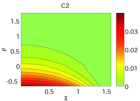
Figure 11: Plots of the metric functions $C$ and $C2$ for $\rho_{0}=-0.71$. Main error of $C2$ originates from the coordinate singularity at $\rho=0,\chi=\pi/2$, but its effect for $C$ through the elliptic equation is small, and the difference of their magnitude is very small compared to $C$.

We reconstruct the values of $A,B$ at the coordinate singularity $\rho=0$, $\chi=\pi/2$ ($C$ of course is zero), and since the $\rho,\chi$ coordinate system is singular there, it is easiest to consider this in the non-singular $r,z$ coordinates. Then from the axial symmetry at $r=0$ and the reflection symmetry at $z=\pi/2$, the metric functions have expansions,

$$A(r,z)=k_{0}+k_{1}r^{2}+k_{2}\,(\pi/2-z)^{2}+O(r^{4},(\pi/2-z)^{4},r^{2}(\pi/2-z)^{2})$$ (35)

and similarly for $B$, and thus using the relation of $r,z$ to $\rho,\chi$, we may simply compute how to interpolate the values at the coordinate singularity $r=0,z=\pi/2$ from the neighbouring points in the $\rho,\chi$ grid.

Appendix B Appendix: Numerical checks

We find second order scaling in all physical quantities such as the mass, temperature and entropy. However, the resolutions are sufficiently high that increases yield very little change in the quantities. Observe the earlier figure 9 where we have plotted the thermodynamic quantities for 3 different resolutions, which give extremely similar results where multiple resolutions may be relaxed. This gives much confidence that the accuracy of these solutions is high. Certainly our main conclusion is seen in this figure, that the black holes become larger in mass and entropy than the most non-uniform strings, and we see this is totally unaffected by changes in resolution.

As discussed in the main text, it is essential to explicitly test that the constraint equations are well satisfied, as these are not imposed directly, but only via boundary conditions and the CR relations. For $\rho_{0}=-0.71$ we plot in figure 12 the weighted constraints $\Psi$ and $\Phi$. We see that they are suitably small, rising to their maximum near the symmetry axis or coordinate singularity. However, it is very difficult to interpret these constraint violation values in terms of their physical effect. A nice check that these small violations are sufficiently small that the physics of the solution is unaffected by them is given in Table 1 where we show the average values of the weighted constraints and $C2-C$ (which also gives a measure of how well $G^{\rho}_{~{}\chi}$ is satisfied) over $\rho$ and $\chi$ for three resolutions with different $\rho_{0}$. As the numerical resolution is increased, the averaged constraint violation values decrease significantly (not quite as quickly as second order scaling, but then our discretisation geometry is rather complicated so this would not be expected), indicating the constraints become increasingly well satisfied, as we would hope for. The geometry and other properties of the solutions varies very little as the resolution is increased, and thus the constraint violations must be very small in terms of their physical effect.

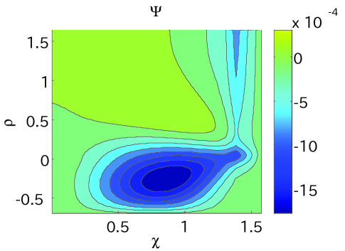
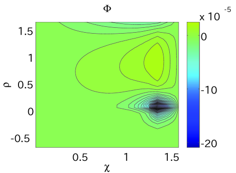
Figure 12: Plots of the weighted constraint equations for $\rho_{0}=-0.71$.

In order to assess the absolute physical error in these small constraint violations globally, we advocate comparing the values of $C$ and $C2$ shown in the previous Appendix over the whole domain. Since these agree extremely well, this is again excellent evidence that $G^{\rho}_{~{}\chi}$ is effectively very well satisfied, since $C2$ is integrated from this constraint, and $C$ is obviously derived from the elliptic equations. Yet another physical test we may perform is to compute the horizon temperature as a function of $\chi$ along the horizon. Again the $G^{\rho}_{~{}\chi}$ constraint should ensure this is constant, yet it is the $(G^{\rho}_{~{}\rho}-G^{\chi}_{~{}\chi})$ constraint that we actually impose at the horizon for the elliptic equations. Thus if $G^{\rho}_{~{}\chi}$ is well satisfied, then the CR constraint structure is working well. In figure 13 we plot the maximum variation, $\delta\mathcal{T}_{error}=\left(\mathcal{T}_{max}-\mathcal{T}_{min}\right)/\mathcal{T}$, of the temperature for varying $\rho_{0}$ for our highest resolution, and two lower resolutions. These variations are small, implying the constraints are indeed well satisfied. Furthermore they decrease very nicely with increasing resolution indicating the constraints are behaving well numerically, and are free from systematic violations. We find maximum variations for the largest black holes, as expected as gradients build up near the horizon at $\chi=\pi/2$ due to the limited resolution at the axis. However the variation is still only $\sim 1\%$ for the largest black hole we relaxed.

In the Table 2 we show the temperature, entropy and mass for a black hole using different $\rho_{max}$. We see these quantities (and indeed all others) hardly change, indicating our choice of $\rho_{max}$ is sufficiently large.

	$\left\langle|\Psi|\right\rangle$	$\left\langle|\Phi|\right\rangle$	$\left\langle|C2-C|\right\rangle$
$\rho_{0}=-1.1$
$140\times 420$	$4.3\times 10^{-5}$	$2.9\times 10^{-6}$	$1.0\times 10^{-5}$
$70\times 210$	$6.6\times 10^{-5}$	$7.2\times 10^{-6}$	$3.1\times 10^{-5}$
$35\times 105$	$1.5\times 10^{-4}$	$1.8\times 10^{-5}$	$8.6\times 10^{-5}$
$\rho_{0}=-0.71$
$140\times 420$	$1.8\times 10^{-4}$	$1.6\times 10^{-5}$	$3.6\times 10^{-5}$
$70\times 210$	$2.6\times 10^{-4}$	$3.2\times 10^{-5}$	$8.6\times 10^{-5}$
$35\times 105$	$5.1\times 10^{-4}$	$5.2\times 10^{-5}$	$1.7\times 10^{-4}$
$\rho_{0}=-0.36$
$140\times 420$	$7.1\times 10^{-4}$	$1.0\times 10^{-4}$	$2.2\times 10^{-4}$
$70\times 210$	$1.2\times 10^{-3}$	$2.1\times 10^{-4}$	$4.3\times 10^{-4}$
$35\times 105$	—	—	—

Table 1: This table shows averaged violations of the weighted constraint equations and $C2-C$ for three resolutions and three different black holes. The average of absolute values is taken over the whole domain.

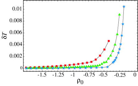
Figure 13: Plot showing the variation of the temperature on the horizon, $\delta\mathcal{T}_{error}=\left(\mathcal{T}_{max}-\mathcal{T}_{min}\right)/\mathcal{T}$, for three resolutions; our maximum 140*420 and two lower resolutions, 70*210 and 36*106.

$70\times 210$	$|\delta\mathcal{T}/\mathcal{T}|$	$|\delta\mathcal{S}/\mathcal{S}|$	$|\delta M/M|$
$\rho_{max}=4.6$	$3.5\times 10^{-4}$	$1.3\times 10^{-3}$	$1.1\times 10^{-2}$
2.5	$3.6\times 10^{-3}$	$1.9\times 10^{-2}$	$9.3\times 10^{-2}$
1.4	$5.1\times 10^{-2}$	$1.8\times 10^{-1}$	$4.0\times 10^{-1}$

Table 2: This table shows the variations of the temperature, entropy and asymptotic mass for a black hole with $\rho_{0}=-0.36$ using different $\rho_{max}$. The variation of the quantities is defined as $\delta\mathcal{T}/\mathcal{T}=1-\mathcal{T}/\mathcal{T}_{\rho_{max}=5.7}$, dividing by $\mathcal{T}$ for $\rho_{max}=5.7$.

Appendix C Appendix: Demonstration that First Law does not test the constraints

In this brief Appendix we demonstrate our claim that deriving the asymptotic mass by integrating the First Law $dM=\mathcal{T}d\mathcal{S}$ along our branch of numerical solutions (for fixed asymptotic radius) does not test whether the constraint equations are satisfied. This is also true for the related Smarr law. Thus while it is useful to check that the First Law is satisfied, as it checks the elliptic equations are well satisfied and have boundary conditions imposed compatibly with their regular singular behaviour, we should not be lulled into a false sense of security. We satisfy the elliptic equations directly in this relaxation method, and to high accuracy, whereas the constraint equations are imposed indirectly, via the boundary conditions. Hence these are the equations we should worry may have numerical errors, and it is crucial to separately check these, as was done in the previous Appendix.

The First Law can be classically derived, eg. as in [56]. Here we simply sketch the derivation, considering which components of the Einstein tensor are involved, and therefore which can be numerically tested by the First Law. Consider the expression,

$$\tilde{S}(g_{\mu\nu})=\int_{\mathcal{M}}d^{6}x\sqrt{-g}R(g_{\mu\nu})$$ (36)

for a manifold $\mathcal{M}$ with metric $g_{\mu\nu}$. This is not the action, since for the action we must subtract the Gibbons-Hawking term at the boundaries $\delta\mathcal{M}$. Clearly $\tilde{S}$ (unlike the true action) vanishes for any solution of the equations of motion, as the Ricci scalar will always vanish locally.

The first law can be derived in our static case by considering $g_{\mu\nu}=g^{(0)}_{\mu\nu}+\delta g_{\mu\nu}$, where $g^{(0)}_{\mu\nu}$ is a static solution of the Einstein equations, and the perturbation $\delta g_{\mu\nu}$ also satisfies the static linearised perturbation equations. Thus, $\tilde{S}$ vanishes when evaluated on both $g^{(0)}$ and $g$. However, in the usual way we can write,

$$\tilde{S}(g_{\alpha\beta})-\tilde{S}(g^{(0)}_{\alpha\beta})=\int_{\mathcal{M}}d^{6}x\sqrt{-g^{(0)}}G_{\mu\nu}(g^{(0)}_{\alpha\beta})\delta g^{\mu\nu}+\left[V_{\mu\nu}\delta g^{\mu\nu}+W_{\mu\nu}\partial_{n}\delta g^{\mu\nu}\right]_{\delta\mathcal{M}}+O(\delta g^{2})$$ (37)

where $\partial_{n}$ is the derivative normal to the boundary, and $V,W$ give boundary terms that arise to eliminate derivatives of $\delta g$ in the integral term. Since the first 3 terms all vanish, we are left simply with the boundary terms, and these give rise to the First Law, linearised in $\delta g$, when evaluated on the horizon and asymptotically. However, let us now consider the above in our numerical context. If numerically we see the First is well satisfied, does this imply all the Einstein equations, both elliptic and constraints, are therefore well satisfied?

Naively this appears so. From the terms $\tilde{S}(g_{\mu\nu})$, $\tilde{S}(g^{(0)}_{\mu\nu})$ we test the weighted average of the Ricci scalars, $R(g)$ and $R(g^{(0)})$, and from the linear variation term we test a weighted average of $G_{\mu\nu}(g^{(0)})$. However, given that our metric (1) is diagonal, and further more, our perturbation $\delta g$ is therefore also diagonal, these three terms then only test the diagonal components of the Einstein tensor. Thus these weighted integrals simply do not involve the $G^{r}_{~{}z}$ Einstein equation (or equivalently $G^{\rho}_{~{}\chi}$). Even worse, due to the conformal invariance of the $r,z$ (or equivalently $f,g$) block of the metric, the perturbation is restricted so $\delta g_{rr}=\delta g_{zz}$ and therefore the integrals also do not involve $(G^{r}_{~{}r}-G^{z}_{~{}z})$ (or equivalently $(G^{\rho}_{~{}\rho}-G^{\chi}_{~{}\chi})$).

Now it is clear that if we take any solution of the elliptic equations, $\tilde{g}^{(0)}$, totally ignoring the constraints, and perturb this by $\delta\tilde{g}$ which again only satisfies the static linearised elliptic equations, we can perform exactly the same manipulations to obtain the above equation, and consequently the usual First Law. Hence for ‘solutions’ only obeying the elliptic equations we would still see the First Law being well observed, even though we had made no attempt to satisfy the constraint equations.

Thus, our specific form of the metric exactly ensures the Einstein equations that are the ‘constraints’ in this elliptic context, $G^{r}_{~{}z}$ and $(G^{r}_{~{}r}-G^{z}_{~{}z})$, do not affect the First Law, even if they are not satisfied due to numerical error. For exactly the same reasons, the closely related Smarr law also has no dependence on the constraint equations, when using our metric choice, and similarly cannot provide a numerical test of the constraints.

References

- [1] L. Randall and R. Sundrum, Phys. Rev. Lett. 83, 4690 (1999), hep-th/9906064.
- [2] T. Kaluza, Sitzungsber. Preuss. Akad. Wiss. Berlin (Math. Phys. ) 1921, 966 (1921).
- [3] O. Klein, Z. Phys. 37, 895 (1926).
- [4] N. Arkani-Hamed, S. Dimopoulos, and G. Dvali, Phys. Lett. B429, 263 (1998), hep-ph/9803315.
- [5] I. Antoniadis, N. Arkani-Hamed, S. Dimopoulos, and G. Dvali, Phys. Lett. B436, 257 (1998), hep-ph/9804398.
- [6] G. Gibbons and D. Wiltshire, Ann. Phys. 167, 201 (1986).
- [7] A. Chodos and S. Detweiler, Gen. Rel. Grav. 14, 879 (1982).
- [8] R. Gregory and R. Laflamme, Phys. Rev. D37, 305 (1988).
- [9] R. Gregory and R. Laflamme, Phys. Rev. Lett. 70, 2837 (1993), hep-th/9301052.
- [10] R. Gregory and R. Laflamme, Nucl. Phys. B428, 399 (1994), hep-th/9404071.
- [11] S. Gubser, Class. Quant. Grav. 19, 4825 (2002), hep-th/0110193.
- [12] T. Wiseman, Class. Quant. Grav. 20, 1137 (2003), hep-th/0209051.
- [13] R. Myers, Phys. Rev. D35, 455 (1987).
- [14] D. Korotkin and H. Nicolai, (1994), gr-qc/9403029.
- [15] A. Frolov and V. Frolov, Phys. Rev. D67, 124025 (2003), hep-th/0302085.
- [16] R. Emparan and H. Reall, Phys. Rev. D65, 084025 (2002), hep-th/0110258.
- [17] T. Harmark and N. Obers, JHEP 05, 032 (2002), hep-th/0204047.
- [18] T. Wiseman, Phys. Rev. D65, 124007 (2002), hep-th/0111057.
- [19] H. Kudoh, T. Tanaka, and T. Nakamura, Phys. Rev. D68, 024035 (2003), gr-qc/0301089.
- [20] H. Kudoh, (2003), hep-th/0306067.
- [21] T. Tanaka, Prog. Theor. Phys. Suppl. 148, 307 (2003), gr-qc/0203082.
- [22] R. Emparan, A. Fabbri, and N. Kaloper, JHEP 08, 043 (2002), hep-th/0206155.
- [23] B. Kol, hep-th/0206220.
- [24] B. Kol, hep-ph/0207037.
- [25] E. Sorkin and T. Piran, Phys. Rev. Lett. 90, 171301 (2003), hep-th/0211210.
- [26] T. Harmark and N. Obers, (2003), hep-th/0309116.
- [27] B. Kol, E. Sorkin, and T. Piran, (2003), hep-th/0309190.
- [28] T. Harmark and N. Obers, (2003), hep-th/0309230.
- [29] T. Wiseman, Class. Quant. Grav. 20, 1177 (2003), hep-th/0211028.
- [30] B. Kol and T. Wiseman, Class. Quant. Grav. 20, 3493 (2003), hep-th/0304070.
- [31] R. Emparan and H. Reall, Phys. Rev. Lett. 88, 101101 (2002), hep-th/0110260.
- [32] B. Kol, hep-th/0208056.
- [33] L. Randall and R. Sundrum, Phys. Rev. Lett. 83, 3370 (1999), hep-ph/9905221.
- [34] A. Chamblin, S. Hawking, and H. Reall, Phys. Rev. D61, 065007 (2000), hep-th/9909205.
- [35] R. Gregory, Class. Quant. Grav. 17, L125 (2000), hep-th/0004101.
- [36] G. Gibbons and S. Hartnoll, Phys. Rev. D66, 064024 (2002), hep-th/0206202.
- [37] T. Tamaki, S. Kanno, and J. Soda, hep-th/0307278.
- [38] S. Gubser and I. Mitra, hep-th/0009126.
- [39] S. Gubser and I. Mitra, JHEP 08, 018 (2001), hep-th/0011127.
- [40] H. Reall, Phys. Rev. D64, 044005 (2001), hep-th/0104071.
- [41] J. Gregory and S. Ross, Phys. Rev. D64, 124006 (2001), hep-th/0106220.
- [42] V. Hubeny and M. Rangamani, JHEP 05, 027 (2002), hep-th/0202189.
- [43] S. Gubser and A. Ozakin, JHEP 05, 010 (2003), hep-th/0301002.
- [44] G. Gibbons, S. Hartnoll, and C. Pope, Phys. Rev. D67, 084024 (2003), hep-th/0208031.
- [45] S. Hartnoll, hep-th/0305001.
- [46] R. Myers and M. Perry, Ann. Phys. 172, 304 (1986).
- [47] H. Reall, Phys. Rev. D68, 024024 (2003), hep-th/0211290.
- [48] R. Emparan and R. Myers, hep-th/0308056.
- [49] G. Horowitz, hep-th/0205069.
- [50] M. Choptuik et al., gr-qc/0304085.
- [51] E. Sorkin, B. Kol, and T. Piran, (2003), hep-th/0310096.
- [52] B. Kleihaus and J. Kunz, Phys. Rev. D57, 834 (1998), gr-qc/9707045.
- [53] M. Choptuik, E. Hirschmann, S. Liebling, and F. Pretorius, Class. Quant. Grav. 20, 1857 (2003), gr-qc/0301006.
- [54] S. Hawking and G. Horowitz, Class. Quant. Grav. 13, 1487 (1996), gr-qc/9501014.
- [55] P. Townsend and M. Zamaklar, Class. Quant. Grav. 18, 5269 (2001), hep-th/0107228.
- [56] R. Wald, Quantum field theory in curved space-time and black hole thermodynamics (Chicago, USA: Univ. Pr. (1994) 205 p), .