hep-th/0310103
Kink-boundary collisions in a two dimensional scalar field theory

In a two-dimensional toy model, motivated from five-dimensional heterotic M-theory, we study the collision of scalar field kinks with boundaries. By numerical simulation of the full two-dimensional theory, we find that the kink is always inelastically reflected with a model-independent fraction of its kinetic energy converted into radiation. We show that the reflection can be analytically understood as a fluctuation around the scalar field vacuum. This picture suggests the possibility of spontaneous emission of kinks from the boundary due to small perturbations in the bulk. We verify this picture numerically by showing that the radiation emitted from the collision of an initial single kink eventually leads to a bulk populated by many kinks. Consequently, processes changing the boundary charges are practically unavoidable in this system. We speculate that the system has a universal final state consisting of a stack of kinks, their number being determined by the initial energy.

1 Introduction

In Ref. [1] we presented a five-dimensional brane-world model, closely related to five-dimensional heterotic M-theory [2, 3, 4, 5, 6], where M-theory five-branes are modelled as kink-solutions of a bulk scalar field theory. We were particularly interested in studying collisions of such kinks with the boundaries, a process which, in the original M-theory model, may lead to a topology-changing so-called small-instanton transition [7, 8] due to absorption of the five-brane. The analysis of Ref. [1] was mainly performed in a moduli space approximation. We concluded that the colliding kink was absorbed by the boundary, however, its final fate could not be determined due to a break-down of the moduli space approach.

In this paper, we will focus on an even simpler, two-dimensional model which captures the essential features of its five-dimensional cousin. The model consists of a ($1+1$)-dimensional scalar field theory for a single real scalar and an associated potential $V$ with (at least) two minima to allow for kink solutions. The spatial direction is taken to be a line segment with the boundary conditions being provided by the “superpotential” [10] $W$ associated to $V$. To simplify the problem we have not included gravity and any other gravity-like fields which were present in the five-dimensional model [1].

Our main goal is to determine the final outcome of the kink-boundary collision using this simple two-dimensional model. In particular, we would like to clarify whether the kink is indeed absorbed or, rather, reflected by the boundary. While the former process would lead to a change in the boundary charge (as measured by the superpotential value) and the number of kinks present in the bulk, the latter process would conserve those numbers. We will mainly approach this problem as one posed within relatively simple two-dimensional scalar field theories whose basic properties we are investigating, although the possible relation to M-theory and topology-changing phenomena is in the back of our minds.

The plan of the paper is as follows. In the next Section, we will set up the model and derive its basic kink solution. Section 3 reviews the moduli space description of kink evolution and kink-boundary collision. The perturbation spectrum on the kink background is analysed in Section 4. In Section 5, we present a full numerical analysis of the two-dimensional model to determine the final outcome of the collision process. An analytic interpretation of the numerical results is given in Section 6. In Section 7, we present a modified moduli space picture which incorporates some, although not all, features of the collision process. We conclude in Section 8 by summarising and presenting some results about the long-time evolution of the system.

2 The model

In this section, we will set up the $1+1$-dimensional model which will be the basis of this paper. This model is designed to capture the essential features of five-dimensional heterotic M-theory [2] and the related defect model presented in Ref. [1] and, at the same time, provide the simplest setting for studying the collision of a kink with a boundary.

Time and spatial coordinate are denoted by $t$ and $x$, respectively, where the latter is taken on a circle, that is, in the range $x\in[-L,L]$ (with the endpoints of the interval identified) subject to the $Z_{2}$ orbifolding generated by $x\rightarrow-x$. The resulting one-dimensional orbifold $S^{1}/Z_{2}$ has two fixed points at $x=x_{1}=0$ and $x=x_{2}=\pm L$ and points $x$ and $-x$ are identified. Instead of working with the full orbicircle, we, therefore, can (and frequently will) use the “downstairs” picture where $x$ is restricted to the interval $x\in[0,L]$. The fixed points at $x_{i}$, where $i=1,2$, can now be thought of as spatial boundaries.

The field content of our model consists of a single real scalar field $\phi$ with a potential $V=V(\phi)$. Gravity and gravity-like fields will not be considered here since they are not essential to analyse the kink-boundary collision. We require the potential to have at least two different minima (with vanishing potential values) in order for kink solutions to exist. We also define the “superpotential” $W$ by

$$W^{\prime}=\sqrt{2V(\phi)}\;.$$ (2.1)

where here and in the following the prime denotes the derivative with respect to $\phi$. We will be interested in actions of the type

$$S=\int{\rm dt}\int_{-L}^{L}{\rm dx}\,\left\{\frac{1}{2}\left(\frac{\partial\phi}{\partial t}\right)^{2}-\frac{1}{2}\left(\frac{\partial\phi}{\partial x}\right)^{2}-V(\phi)-2\delta(x-0)\,W(\phi)+2\delta(x-L)\,W(\phi)\right\}$$ (2.2)

The equations of motion and boundary conditions in the boundary picture are then given by

$$\frac{\partial^{2}\phi}{\partial t^{2}}=\frac{\partial^{2}\phi}{\partial x^{2}}-V^{\prime}(\phi),\qquad\qquad\left.\frac{\partial\phi}{\partial x}\right|_{x_{i}}=\left.W^{\prime}(\phi)\right|_{x_{i}}\;.$$ (2.3)

For the numerical simulations and for concreteness we will often use the quartic potential

$$V(\phi)=\frac{1}{8}g^{2}(\phi^{2}-v^{2})^{2}$$ (2.4)

with associated superpotential

$$W=-\frac{1}{2}g\left(\frac{1}{3}\phi^{3}-\phi v^{2}\right)\;.$$ (2.5)

The form of the boundary terms in the action (2.2) has been chosen to facilitate the existence of BPS solutions. This can be understood by focusing on static configurations $\phi=\phi(x)$. For such configurations, the action can be written as

$$S\sim\int_{0}^{L}dx\left(\frac{d\phi}{dx}-W^{\prime}\right)^{2}\;.$$ (2.6)

Note that the boundaries terms which arise from partial integration when converting the action (2.2) into the above form are precisely cancelled by the original boundary terms in (2.2). Hence, we find static solutions $\phi=\phi(x)$ of our action satisfy the first order equation

$$\frac{d\phi}{dx}=W^{\prime}\;.$$ (2.7)

Conversely, solutions to this first order equation clearly satisfy the boundary conditions as well as the second-order equation of motion in (2.3), the latter by virtue of the relation between $V$ and $W$.

From eq. (2.7), the solution $\phi_{\rm K}$ of a kink can in general be written as

$$\phi_{K}(x)=f(x-Z)\;,\qquad f^{-1}(\phi)=\int_{\phi_{0}}^{\phi}\frac{d\tilde{\phi}}{W^{\prime}(\tilde{\phi})}\;.$$ (2.8)

Here we take $\phi_{0}$ to be the $\phi$ value at the core of the kink, corresponding to the maximum of the potential. Then, the constant $Z$ can be interpreted as the position of the kink’s core as long as $Z\in[0,L]$. For $Z$ outside this range, the core of the kink is no longer within the physical part of space and $Z$ merely indicates the “virtual” position of the core.

For the quartic potential (2.4) the kink solution is given by

$$\phi_{\rm K}(x)=v\;\tanh\left(\frac{x-Z}{2L_{\rm K}}\right)$$ (2.9)

where the width $L_{\rm K}$ of the kink is given by

$$L_{\rm K}=\frac{1}{gv}\;.$$ (2.10)

As long as kinks are sufficiently away from the boundaries, the field $\phi$ will be close to minima of its potential $V$ on the boundaries. Then, the boundary superpotential takes values from a discrete set consisting of the values $W$ assumes at the minima of the potential $V$. These discrete values can be interpreted as boundary charges. They are analogous to the topological boundary charges which appear in the related M-theory model [2, 1]. In order to consistently maintain this interpretation, the superpotential must be monotonically increasing, and so Eq. (2.5) is only valid for $-v<\phi<v$.

We note that our boundary conditions are related to the family considered in [9]. These papers studied integrable ($1+1$)-dimensional field theories on the half line, including the sine-Gordon theory, with a two-parameter set of boundary conditions $\phi^{\prime}=MW^{\prime}(\phi-\phi_{0})$ at the origin. The fact that these boundary conditions do not spoil the integrability generated considerable interest.

3 Moduli space evolution

In the previous section, we have presented a one-parameter family of static BPS kink solutions for our theory (2.2) which is labelled by the parameter $Z$. Solutions exist for all values $Z\in[-\infty,\infty]$ but only for $Z\in[0,L]$ does $Z$ correspond to the position of the kink’s core. Otherwise, the kink’s core is located “outside” and only its tail remains within the physical part of space. Values $Z=0$ or $Z=L$ correspond to a kink with its core being exactly located at one of the boundaries.

We would now like to consider physical motion in this moduli space of kinks by promoting $Z$ to a slowly-varying function of time, $Z=Z(t)$. A time evolution $Z\rightarrow 0_{+}$ ($Z\rightarrow L_{-}$) then describes the collision of the kink with the boundary at $x=x_{1}=0$ ($x=x_{2}=L$) which is the process we would like to study in this paper. For definiteness, we will focus on collisions with the boundary at $x=0$ in the following but the conclusions, of course, apply to collisions with the other boundary at $x=L$ as well.

The one-dimensional effective theory $S_{\rm eff}$ for the modulus $Z=Z(t)$ can be obtained by inserting the kink-solution (2.8) into the action (2.2) and integrating over the spatial coordinate. This results in

$$S_{\rm eff}=\int\ dt\,F(Z)\,\dot{Z}^{2},$$ (3.1)

where the function $F=F(Z)$ is given by

$$F(Z)=W(f(L-Z))-W(f(-Z))\;.$$ (3.2)

The last equation means that $F$ is the difference of the boundary superpotentials evaluated on the kink solution. From this interpretation the qualitative behaviour of $F$ can be easily inferred. For $Z\in[0,L]$ and well away from the boundaries (that is, away by more than the width of the kink) the field $\phi_{\rm K}$ is very close to neighbouring minima of the potential on the two boundaries. More precisely, $\phi_{\rm K}(x=0)$ is very close to the minimum with the smaller superpotential value and $\phi_{\rm K}(x=L)$ is very close to the neighbouring minimum with the larger superpotential value. This means, for such values of $Z$ the function $F(Z)$ is finite positive and approximately constant. On the other hand, for $Z<0$ or $Z>L$ and away from the boundary, $\phi$ is very close to the same minimum for both boundaries which means that $F(Z)$ is approximately zero (although still positive).

The function $F$ can be computed for any given potential $V$ and associated superpotential $W$ to confirm this expectation. For the quartic potential (2.4), the associated superpotential (2.5) and kink solution (2.9) one finds

$$F(Z)=gv^{3}\left.\left[\tanh(\frac{g}{2}v\,(x-Z))-\frac{1}{3}\tanh^{3}(\frac{g}{2}v\,(x-Z))\right]\right|_{0}^{L}\;.$$ (3.3)

This function has been plotted in Fig. 1 and it shows indeed the general properties discussed above. The constant value of $F$ for $Z$ inside the interval is given by

$$F(Z)\simeq 4gv^{3}/3\;\;{\rm for}\;\;Z\gg L_{\rm K}\;\;{\rm and}\;\;L-Z\gg L_{\rm K}\;.$$ (3.4)

For later purposes, it is also useful to note the asymptotic behaviour of $F$ for $Z\ll-L_{\rm K}$ which will be relevant after a collision of the kink with the boundary at $x=0$. It is given by

$$F(Z)\simeq 4gv^{3}\,\left(1-e^{-2gvL}\right)\,e^{2gv\,Z}\;\;{\rm for}\;\;Z\ll-L_{\rm K}\;.$$ (3.5)

If the width of the kink $L_{\rm K}$ is much smaller than the size $L$ of the interval, $L_{\rm K}\ll L$, this reduces to

$$F(Z)\simeq 4gv^{3}\,e^{2gv\,Z}\;\;{\rm for}\;\;Z\ll-L_{\rm K}\;\;{\rm and}\;\;L_{\rm K}\ll L\;.$$ (3.6)

The equations of motion derived from the effective action (3.1) are simply

$$\frac{d}{dt}\left(F\dot{Z}^{2}\right)=0\;,$$ (3.7)

where the dot denotes the derivative with respect to time. This leads to the first integral

$$F\dot{Z}^{2}=u^{2}={\rm const}\;,$$ (3.8)

where $u$ is a constant. This relation, of course, represents energy conservation. Together with the properties of $F$ stated above it implies that $Z$ evolves with constant velocity in the interval $Z\in[0,L]$ and, once it has collided with the boundary at $x=0$, accelerates and evolves towards $Z\rightarrow-\infty$ while $\dot{Z}$ diverges. Moreover, from the explicit form of $F$ one can show that $Z$ reaches $-\infty$ in a finite time. Of course, the validity of the effective theory (3.1) when $Z$ and $\dot{Z}$ diverge after a collision is at best doubtful. Although the effective theory provides a good description of slow kink motion for finite values of $Z$, it seems difficult, therefore, to draw any reliable conclusion about the outcome of the collision based on this effective theory. Three possibilities are conceivable. The kink could be absorbed by the boundary with its kinetic energy being completely converted into radiation (that is, fluctuations of $\phi$ around one of its vacuum states). In this case the charge on the absorbing boundary would have changed by one unit between the initial and final state. It could be inelastically reflected with part of its kinetic energy being transferred to radiation or it could be elastically reflected. Then the boundary charge remains unchanged. We will now analyse the full two-dimensional theory (2.2) to determine which of these three possibilities is actually realised.

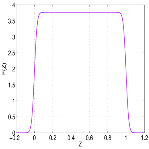
Figure 1: The function F(Z) for an interval with length $L=1$ and a kink width of $L_{\rm K}=\frac{1}{32\sqrt{2}}$.

4 Perturbation spectrum

It is instructive to examine how the eigenfunctions and eigenvalues of small perturbations around the kink change with the modulus $Z$. To find the eigenvalues we must expand the field around the kink configuration $\phi(x)=\phi_{\rm K}(x-Z)+\varphi(x)$ and solve the eigenvalue problem

$$\left[-\frac{d^{2}}{dx^{2}}+V^{\prime\prime}(\phi_{\rm K})+2W^{\prime\prime}(\phi_{\rm K})\delta(x)\right]\varphi=\omega^{2}\varphi$$ (4.1)

Here, we have neglected the contribution from the boundary at $x=L$ which is justified as long as the kink is sufficiently far away from this boundary. This can always be achieved by making $L$ large. We would then expect that at large positive $Z$, the spectrum would be asymptotically close to that of an isolated kink [12]. For the quartic potential (2.4) one expects one zero mode with no nodes, a bound state with one node and eigenvalue $\omega_{1}^{2}=3\mu^{2}/2$, and a continuum starting at $\omega_{2}^{2}=2\mu^{2}$, where $\mu=gv/\sqrt{2}$. At large negative $Z$, the spectrum should be asymptotically close to that of the vacuum, which also possesses a nodeless zero mode and a continuum starting at $\omega^{2}=2\mu^{2}$, but no bound state.

Although the free kink eigenfunctions and eigenvalues are known exactly [12], the non-trivial boundary condition, or equivalently the extra $\delta$-function contribution to the potential, change the problem. As we have not been able to find a solution to the eigenvalue problem in closed form, we resorted to a simple numerical method.

Eq. (4.1) was discretised on an $2N+1$-point interval $-L<x<L$, using the lowest order discrete Laplacian

$$-\frac{d^{2}}{dx^{2}}(y)\to-\frac{\varphi_{i+1}-2\varphi_{i}+\varphi_{i-1}}{\Delta x^{2}},$$ (4.2)

where $\Delta x=L/N$. At the left (right) boundary the double forward (backward) derivative was taken, which improves the accuracy at the expense of generating two spurious eigenfunctions with large negative eigenvalues. The $\delta$-function was defined as $\delta(x)\to\delta_{i0}/\Delta x$. One should note that in defining the problem for both positive and negative values of $x$, we will find eigenfunctions which are both symmetric and antisymmetric under reflections around $x=0$. We are clearly interested only in the symmetric ones.

The eigenfunctions and eigenvalues are easily found using matlab. We took $N=100$ and $L=10$, in units where $\mu=1$. The lowest three (0, 1 and 2 nodes) are shown for $-2<Z<2$ in Fig. (2). The closeness of the lowest eigenvalue to 0 is a measure of the accuracy of the procedure. The shapes of the eigenfunctions for $Z=-2$, $Z=0$ and $Z=2$ are shown in Fig. (3).

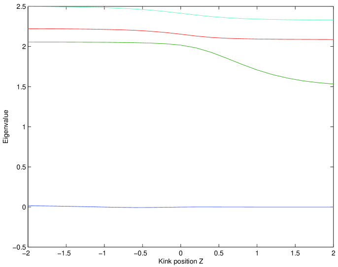
Figure 2: The lowest three eigenvalues $\omega^{2}$ as a function of kink position $Z$. As $Z$ decreases, the bound state at $\omega^{2}=1.5$ moves towards the continuum at $\omega^{2}=2$. In infinite volume it will remain bound, but exponentially weakly.

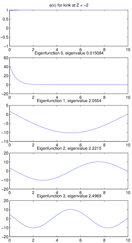
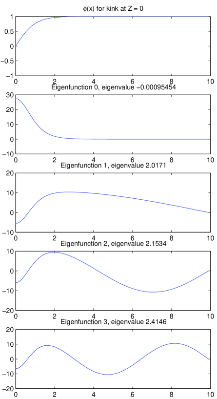
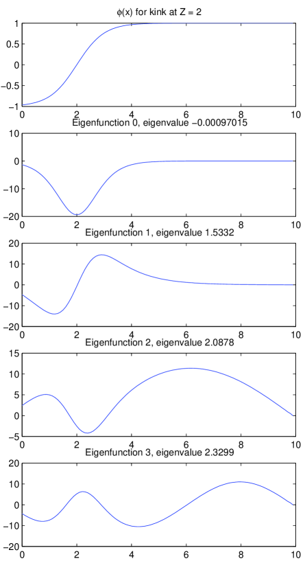
Figure 3: Graphs of the eigenfunctions corresponding to the lowest three eigenvalues for the kink at (a) $Z=-2$, (b) $Z=0$, and (c) $Z=2$. At the top is a graph of the field $\phi$ itself.

As we will see later, the existence of a zero mode for all values of the kink position $Z$ is crucial for an understanding of the kink-boundary collision. We will also find that it has important implications for the creation of kinks due to spontaneous emission from the boundary.

5 Numerical Simulation

As we have seen in the previous sections, a straightforward moduli calculation suggests that, as the kink collides with the boundary, it should cross it and accelerate towards infinity. As a result, the field configuration inside the bulk will approach one of the true vaccua of the theory. We could then expect the kinetic energy of the kink to be converted into radiative excitations of the vacuum that would propagate away from the boundary. This reasoning suggests, the kink should be absorbed by the boundary as a result of the collision. In this section we will test this expectation by performing numerical simulations of the kink/boundary collision. As we will see, a more complex picture will emerge, showing how the moduli description fails to capture the essential features of the collision process.

We model the bulk equation of motion Eq. (2.3) with the quartic potential (2.4) on a $1D$ lattice using a second order discretization of the Laplacian operator, and propagate it in time according to a standard leapfrog algorithm. The implementation of the boundary condition is less straightforward, since it relates a function of the field to its spatial derivative. Taking as an example the boundary condition at $x=0$, we discretise it as

$$\frac{\phi_{1}-\phi_{0}}{\delta x}=W^{\prime}(\phi_{m}),$$ (5.1)

where $\phi_{m}$ is the value of the field evaluated at some point in the interval $(0,\delta x)$. We allowed for different choices of the discretization scheme by writing $\phi_{m}=(1-G)\,\phi_{0}+G\,\phi_{1}$, with $G$ a parameter lying between $0$ and $1$. Since the discretised spatial derivative is effectively evaluated in the mid-point between lattice sites $i=0$ and $i=1$, the most natural option is to set $G=.5$ We confirmed that this choice is the most accurate one, by evolving in time a stationary kink configuration, with its core placed near the boundary. For $G>.5$ the kink is slightly repelled by the boundary, whereas for $G<.5$ the boundary has an attractive effect. The disadvantage of setting $G=.5$ is that it turns Eq. (5.1) into a non-linear implicit equation for $\phi_{0}$, which has to be solved numerically for each time-step. This is clearly the case for any choice of $G$ other than $G=1$. On the other hand, for the lattice action obtained by a straightforward discretization of Eq. (2.2), the only energy conserving algorithm corresponds to $G=0$. For $G>0$ we cannot rely on energy conservation as test of the adequacy of the choice of time-step. Of course all schemes conserve energy in the $\delta x\rightarrow 0$ limit. Since we are dealing with a one-dimensional system, we had no serious computational restrictions and we chose to work with $G=.5$. We have checked that, in the limit of small lattice spacing the three values $G=0,.5$ and $1$ lead to the same results. The boundary condition equation Eq. (5.1) was solved using an implementation of the Newton-Raphson method (see [13]).

The initial conditions for the numerical evolution should model, as closely as possible, a kink in the bulk with a given velocity $\dot{Z}_{i}$ moving towards one of the boundaries. We set up the initial field configuration as $\phi_{K}(x-Z_{i})$ using the kink profile in Eq. (2.9), with $Z_{i}$ the initial core position far from both boundaries. The initial field momentum is defined as $\Pi=-\dot{Z}_{i}\,\partial_{x}\phi_{K}$, where $\dot{Z}_{i}$ is the chosen initial kink velocity. The simulations were run for a theory with $g=2\sqrt{2}$ and $v=1$, which implies a kink width of $L_{\rm K}=\frac{1}{2\sqrt{2}}$. We chose a box of physical length $L=16$, comfortably larger than the kink width. For high and mid-range kink velocities, the lattice parameters were set to $\delta x=.0125$ and $\delta t=.005$. Low collision velocities lead to a large total simulation time and a smaller time-step is needed to avoid error accumulation. For the lowest velocities we used $\delta x=.00125$ and $\delta t=.001$.

We explored a wide range of collision velocities, letting $\dot{Z}_{i}$ vary between $.01$ and $.75$ in steps of $.01$ In Fig. 4 we can see a series of snapshots of $\phi$ for several evolution times in a typical run (in this case $\dot{Z}_{i}=.3$). During the first part of the evolution the kink moves towards the boundary with constant velocity. As its core starts moving into the boundary there is, as expected from the moduli picture, an increase in $\dot{Z}$. At some point the kink leaves the bulk completely and the field is left in the true vacuum, oscillating rapidly in the vicinity of the boundary. The kink then “returns” into the simulation box, moving away from the boundary with decreasing velocity at first. When its core is well inside the bulk the kink velocity oscillates around an average value $\dot{Z}_{f}$. This final value is always smaller than the initial velocity $\dot{Z}_{i}$, as some energy is lost into radiation during the collision. In the late time profiles in Fig. 4 we can see these radiative perturbations moving away from the boundary.

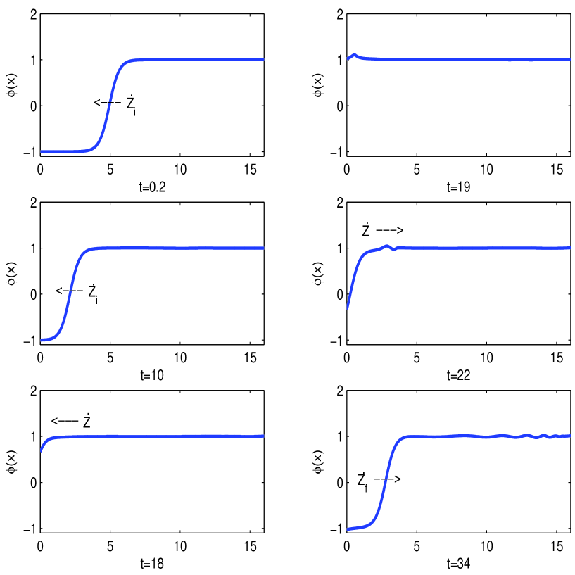
Figure 4: Kink collision for initial velocity $\dot{Z}_{i}=0.3$. In the first two snapshots, $t=.2$ and $t=10$, the kink moves towards the boundary with approximately constant velocity. For $t=18$ most of the core has already crossed the boundary, although the profile inside the bulk remains relatively undistorted. For $t=19$ the field oscillates around the true vacuum. These perturbations propagate away at the speed of light, as seen in the next two plots. At $t=22$ the kink core has re-entered the bulk, and in the final plot we can see the final kink profile, moving away from the boundary with constant velocity.

In Fig. 5 we have a plot of the kink velocity versus time. $\dot{Z}(t)$ was evaluated by numerical differentiation of the position of the core of the kink $Z(t)$. This in turn was defined as the position of the zero of the field, obtained by interpolating $\phi$ as its sign changes. The same features of the evolution can be seen, with $\dot{Z}(t)$ increasing as the kink approaches the boundary, and being reflected later on with a lower final velocity. Note that in both the beginning and end periods of the evolution, the velocity is not strictly constant, oscillating around an average value. This indicates that in both cases, apart from the translational mode, other modes of the kink are excited. As far as the initial condition is concerned this was expected since we are not using a Lorentz boosted kink, which would clearly not obey the boundary conditions. This effect is particularly visible for high kink velocities, both before and after the collision.

Surprisingly, the overall qualitative pattern of the evolution did not change within the whole range of velocities observed. Even for very low velocities, where we expected the reasoning based on the moduli calculation to be applicable, the incoming kink was always reflected by the boundary after the collision. In the next few sections we will try to explain this behaviour and gain a deeper quantitative understanding of the collision process.

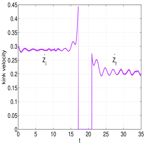
Figure 5: Kink velocity versus time for initial velocity $\dot{Z}_{i}=0.3$. As predicted by the moduli calculation, the kink accelerates as it approaches the boundary. After the collision it returns into the bulk with a lower final velocity. During the collision period, when the core is outside the bulk, the kink position cannot be determined by the zero of the field, and we have defined the kink velocity as zero.

6 Collision as a vacuum perturbation

As we have seen in Section 3, the motion of the kink should be well described by the moduli equations of motion, up to the point when the velocity of its core becomes too large. For low values of the initial velocity $\dot{Z}_{i}$, we expect this to happen when the kink core is outside the bulk and far from away from the boundary. That this is the case can be easily shown using the moduli energy conservation equation (3.8). Assuming that the moduli approximation breaks down for velocities above a certain $\dot{Z}_{max}$. Then Eq. (3.8) implies that the corresponding core position $Z_{max}$ should satisfy

$$F(Z_{max})=\frac{4}{3}gv^{3}\left(\frac{\dot{Z}_{i}}{\dot{Z}_{max}}\right)^{2}\;.$$ (6.1)

Here we assumed the kink to be initially inside the bulk and far from its boundaries so that (3.4) applies. Clearly, the form of $F(Z)$ implies that for $\dot{Z}_{i}$ small enough, $Z_{max}$ can be made arbitrarily large.

If, when the maximal velocity is reached, we have $Z_{max}\ll-L_{\rm K}$, the field configuration in the bulk will be everywhere very close to the vacuum $v$. This suggests that for low $\dot{Z}_{i}$, we could use the linearised equations of motion around $v$ to describe the evolution, after the moduli approximation breaks down. In this section we will use this approach to show that the kink bounces back inelastically after the collision, confirming the previous simulation results.

6.1 Expansion basis for linearised equations of motion

As discussed above we perturb around the vacuum $v$ and write $\phi=\varphi+v$. For small $\varphi$ the field equation of motion reduces to

$$\ddot{\varphi}=\varphi^{\prime\prime}-m^{2}\varphi$$ (6.2)

where $m=gv$ in the case of the quartic potential. The non-trivial contribution to the evolution will come from the boundary condition, which is given by

$$\varphi^{\prime}(x_{i},t)=(g/2)\,|\,\phi^{2}(x_{i},t)-v^{2}|=m\,|\,\varphi(x_{i},t)|$$ (6.3)

In this section we will focus on a collision taking place at the left boundary, $x=0$, and effectively assume the bulk to be half-infinite. This should be a reasonable approximation as long as the size of the bulk is larger than the collision time, so that effects from the radiation produced during collision reaching the opposite boundary can be neglected. Note that, as a consequence of the norm in (6.3), the boundary condition for $\varphi$ is non-linear. Nevertheless, for periods of the evolution during which $\varphi$ does not change sign at the origin, (6.3) reduces to a linear equation. In particular we have

$$\varphi^{\prime}(0,t)=m\,\varphi(0,t),\,\,\,\,\,\,\,\, {\rm if} \varphi(0,t)>0,$$ (6.4)

$$\varphi^{\prime}(0,t)=-m\,\varphi(0,t),\,\,\,\,\,\,\,\, {\rm if} \varphi(0,t)<0\;.$$ (6.5)

This implies that we can still expand arbitrary solutions of (6.2) and (6.3) in terms of given mode functions, as long as we use a different basis for different periods of the evolution. We start with the case $\varphi(0,t)>0$. A complete basis of solutions of (6.2) satisfying (6.4) is given by

$$\varphi_{k}(x,t)=N_{k}\,e^{\pm i\omega t}\,\left[\cos(kx)+\frac{m}{k}\sin(kx)\right],\,\,\,\,\,\,w^{2}=k^{2}+m^{2},\,\,\,\,k>0\;.$$ (6.6)

To obtain the normalisation coefficient we define the mode functions in a finite box of size $L$, leading to $N_{k}^{2}=2k^{2}/(L\omega^{2})$. In the end of the calculation we will take $L\rightarrow\infty$. As for $k$, it will have a discrete spectrum depending on the boundary conditions on the right end of the box. For simplicity we chose periodic boundary conditions, implying $\cos(kL)+(m/k)\,\sin(kL)=1$. As the box size is taken to infinity this should not be relevant for the final result.

In the case of negative field values $\varphi(0,t)$ the basis is given by

$$\varphi_{k}(x,t)=N_{k}\,e^{\pm i\omega t}\,\left[\cos(kx)-\frac{m}{k}\sin(kx)\right],\,\,\,\,\,\,w^{2}=k^{2}+m^{2},\,\,\,\,k>0$$ (6.7)

with $\cos(kL)-(m/k)\,\sin(kL)=1$. Here $N_{k}^{2}$ is a normalisation which will be unimportant for the subsequent calculation. In addition, for the case of negative field values $\varphi(0,t)$ and only for this case, there is also a zero-mass solution of the general form

$$\varphi_{0}(x,t)=(a+b\,t)\,e^{-mx}$$ (6.8)

This zero mode corresponds to the tail of the kink when its core is far outside the bulk. It can be seen as the linearised version of the translational zero mode of the kink. As we will see, this is the essential feature that distinguishes the evolution in the two regimes, $\varphi>0$ and $\varphi<0$.

6.2 Linear solution

We now apply the above results to the kink/boundary collision situation. For simplicity, we define $t=0$ as the time when the moduli approximation breaks down. For this time, we must find the corresponding field configuration inside the bulk which can then be taken as initial condition for the equations of motion linearised around the vacuum. When the kink core is very far from the boundary, the bulk field and its time derivative can be approximated by

$$\phi(x,t) = v-2v\,e^{mZ(t)}\,e^{-mx}$$ (6.9)

$$\partial_{t}\phi(x,t) = -2mv\,\dot{Z}(t)\,e^{mZ(t)}\,e^{-mx}$$ (6.10)

We will assume that we can neglect the small perturbation around the vacuum and that effectively $\phi=v$ in the bulk at $t=0$. The derivative term on the other hand, remains finite even as $\dot{Z}(t)$ diverges. Using energy conservation (3.8) and (3.6) we obtain

$$4mv^{2}\,e^{2mZ}\,\dot{Z}^{2}=F(Z_{i})\,\dot{Z_{i}}^{2}$$ (6.11)

which implies, using the asymptotic expansion for $F(Z)$, that

$$e^{mZ}\,\dot{Z}=\frac{\dot{Z}_{i}}{\sqrt{3}}\;.$$ (6.12)

This allows us to express the finite amplitude of the velocity profile at collision time in terms of the initial velocity of the kink. The perturbation field at $t=0$ is then defined as

$$\varphi(x,0) = 0$$ (6.13)

$$\dot{\varphi}(x,0) = -\frac{2}{\sqrt{3}}\,mv\,\dot{Z}_{i}\,e^{-mx}$$ (6.14)

These are now to be taken as initial conditions of the linearised equations of motion. Since $\dot{\varphi}>0$ we will be entering a phase of the evolution for which $\varphi(0,t)>0$ and we should expand (6.14) in terms of the corresponding basis (6.6). The expansion coefficients are easily obtained (the result depends only on integrals of products of exponentials and trigonometric functions) leading to

$$\varphi(x,t)=\frac{4A}{L}m\,\left(1-e^{-mL}\right)\,\sum_{k}\frac{k^{2}}{\omega^{5}}\,\sin(\omega t)\,\left[\cos(kx)+\frac{m}{k}\sin(kx)\right]$$ (6.15)

where $A=(2/\sqrt{3})mv\,\dot{Z}_{i}$ is the amplitude of the exponential tail in the initial velocity profile for the field.

Equation (6.15) is only valid as long as $\varphi(0,t)>0$. When the field becomes negative at the origin, the boundary condition changes sign and the solution should then be expanded in terms of the second basis (6.7). Let us define a “reflection time” $t_{R}$, for which the solution becomes negative at the boundary, that is $\varphi(0,t_{R})=0$. We can use (6.15) to calculate explicitly the mode amplitudes of $\varphi(x,t_{R})=0$ in terms of the $\varphi<0$ basis. The new ingredient now is the presence of the zero mode. All other modes are oscillatory, corresponding to the radiation that will propagate away from the boundary after the collision. The zero mode $\varphi_{0}$ on the other hand, will grow linearly in time, becoming the tail of the incoming kink. The situation will now mirror what happened before the collision, with the amplitude of the massless mode being related to the final velocity of the reflected kink $Z_{f}$. We define the zero mode amplitude as

$$a_{0}=\int dx\,\,\partial_{t}\varphi(x,t_{R})\,N_{0}\,e^{-mx}$$ (6.16)

where $N_{0}^{2}=2m/(1-e^{-2mL})$ is the corresponding normalisation factor. The time derivative of the field at $t_{R}$ will be given by:

$$\dot{\varphi}(x,t_{R})=a_{0}\,N_{0}\,e^{-mx}+\,{\rm oscillatory\,\,terms}$$ (6.17)

Since we are mainly interested in determining the final velocity of the reflected kink, we will not calculate explicitly the positive $k$ component of the field. We define the amplitude of the exponential term in $\dot{\varphi}(x,t_{R})$ as $B=a_{0}\,N_{0}$, and in analogy with the calculation for the kink before the collision, (6.14) leads to

$$\dot{Z}_{f}=\frac{\sqrt{3}}{2mv}\,B\;.$$ (6.18)

A reflection coefficient can be defined as $R=\dot{Z}_{f}/\dot{Z}_{i}=B/A$, quantifying the elasticity of the collision. The amplitude $B$ can be easily obtained by performing the integral in Eq. (6.16), leading to the expression

$$R=\frac{B}{A}=N_{0}^{2}\,\,\frac{2}{L}\,\left(1-e^{-mL}\right)^{2}\,4m^{2}\,\sum_{k}\frac{k^{2}}{\omega^{6}}\,\cos(\omega t_{R})\,$$ (6.19)

for the reflection coefficient where $\omega$ is given in Eq. (6.6). Note that this solves the problem. We have obtained a formula for the reflection coefficient in terms of the reflection time $t_{R}$, which, in turn, is implicitly determined by Eq. (6.15) as the time satisfying $\varphi(0,t_{R})=0$.

6.3 Comparison with numerical data

To evaluate exact numerical values it is convenient to approximate the series obtained in the previous section by integrals. There is a slight subtlety involved, related to the fact that we must add over all values of $k$ that solve the periodic boundary condition $\cos(kL)+(m/k)\,\sin(kL)=1$. This equation is solved by $k=2n\pi/L$, and by an extra non-trivial solution in every interval $(2n\pi/L,2(n+1)\pi/L)$. This second solution approaches $k=2n\pi/L$ as $n\rightarrow\infty$. In replacing sums over $k$ by integrals we must take into consideration the fact that there are two $k$’s in each interval of length $2\pi/L$ and use $(\pi/L)\sum_{k}\rightarrow\int dk$ (rather than $(2\pi/L)\sum_{k}\rightarrow\int dk$). Using the continuum version of (6.19) we obtain for the reflection coefficient

$$R=\frac{16m^{3}}{\pi}\,\int_{0}^{\infty}dk\,\frac{k^{2}}{\omega^{6}}\,\cos(\omega t_{R})$$ (6.20)

The reflection time $t_{R}$ is given implicitly by

$$\int_{0}^{\infty}dk\,\frac{k^{2}}{\omega^{5}}\,\sin(\omega t_{R})=0$$ (6.21)

Both integrals can easily be re-scaled and evaluated numerically, leading to the final results:

$$t_{R}=\frac{2.06}{m},\,\,\,\,\,\,\,R=0.63$$ (6.22)

These compare very well with the simulation results in the limit of low collision velocities, as illustrated in Figs. 6 and 7. As the initial kink velocity increases deviations from the analytical result can be observed. This is to be expected, since for higher velocities the moduli approximation should break down earlier, making equation (6.14) a worse guess for the form of the initial conditions for the linear regime. Also, we should expect corrections to the linear approximation as the field starts probing the non-linearities of the potential during the collision, for high $\dot{Z}_{i}$. Still, in the particular system simulated, the numerical results remain within 10% of the analytical prediction for velocities up to $\dot{Z}_{i}=0.3$.

It is interesting to note that the equation (6.22) depends only on the mass of the perturbed theory around the vacuum. In fact, it is easy to see that the derivation leading to this result could be reproduced for a general potential with non-vanishing second order derivative at the true vacuum. In particular, for this class of potentials, the reflection coefficient should be model independent. We confirmed this remarkable result by simulating a few collision velocities for a sine-Gordon model. As expected, we observed $R=0.63$.

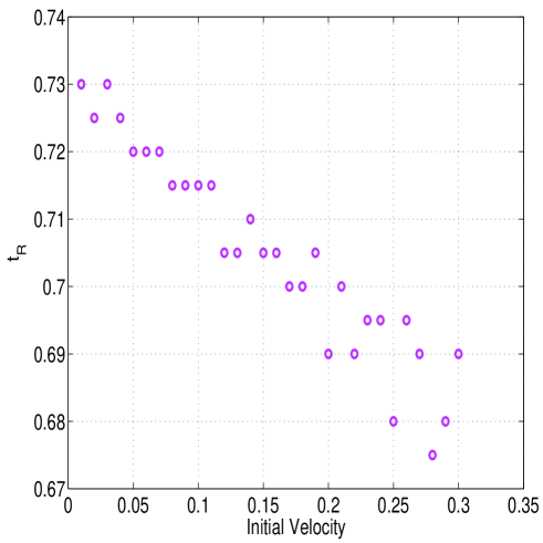
Figure 6: Reflection time versus collision velocity for a model with $g=2\sqrt{2},\,\,v=1,\,\,m=2\sqrt{2}$. The theoretical prediction (6.22) for this choice of parameters is $t_{R}=0.73$. The reflection time $t_{R}$ was defined as the length of time for which $\phi(0,t)>v$ for each simulation.

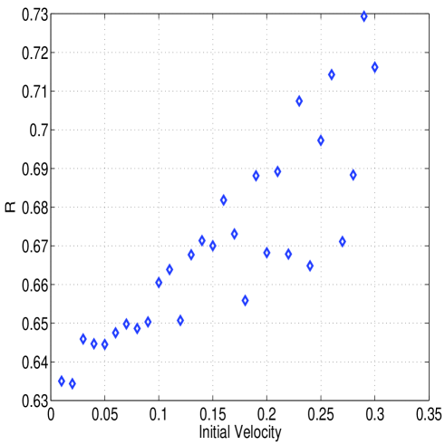
Figure 7: Reflection coefficient versus collision velocity for $g=2\sqrt{2},\,\,v=1,\,\,m=2\sqrt{2}$. The (model independent) analytical prediction is $R=0.63$. Both the initial and final velocities were determined by fitting the position of the core of the kink (as defined in Section 5) to a straight line in the relevant regimes.

7 Moduli space interpretation of the kink-boundary collision

Can we find an interpretation for our results in terms of a suitable modification of the one-dimensional moduli-space approximation described in Section 3? As before, we focus on a collision with the boundary at $x=0$. In view of the effective action (3.1), it seems natural to introduce a new field $\zeta$ with a canonically normalised kinetic term by setting

$$\frac{d\zeta}{dZ}=\pm\sqrt{F}\;,\qquad\zeta(Z)=\pm\int_{-\infty}^{Z}d\tilde{Z}\sqrt{F(\tilde{Z})}\;.$$ (7.1)

Note that the integral in this definition is indeed finite which corresponds to the fact that $Z$ reaches $-\infty$ in a finite time. For a positive (negative) sign in the above definition the full range of $Z$ values is mapped into positive (negative) $\zeta$ values while the point $Z=-\infty$ is mapped to $\zeta=0$ for both signs. The effective action (3.1) now takes the canonical form

$$S_{\rm eff}=\int dt\,\dot{\zeta}^{2}$$ (7.2)

and leads to the first integral

$$\dot{\zeta}=V={\rm const}\;.$$ (7.3)

Let us discuss the collision process in terms of the new field $\zeta$. We start off at some finite, positive value $\zeta$, corresponding to the kink being located between the boundaries, and move with a constant, negative velocity towards $\zeta=0$. When $\zeta$ reaches some smaller, positive value, corresponding to the position of the boundary at $x=0$, the collision takes place. From there $\zeta$ continues to evolve to zero and, finally, into negative values. Nothing special happens at $\zeta=0$ which corresponds to the formerly problematic point $Z=-\infty$. We would now like to re-interpret this evolution of $\zeta$ in terms of our original field $Z$. Note that, from Eq. (7.1) we have

$$\dot{Z}=\left\{\begin{array}[]{rrr}+\frac{V}{\sqrt{F}}&{\rm for}&\zeta>0\\ -\frac{V}{\sqrt{F}}&{\rm for}&\zeta<0\end{array}\right.\;.$$ (7.4)

This means crossing of $\zeta=0$ after a collision implies a sign change in the velocity of $Z$ and, hence, a reflection of the kink. This is precisely what we have found in the full two-dimensional theory. An alternative way of stating this is to note that $\zeta$ is really defined on $R/Z_{2}$. Here the $Z_{2}$ identifies $\zeta$ and $-\zeta$ which correspond to the same field value $Z$. In fact, upon including the other boundary the $\zeta$ moduli space is, perhaps not surprisingly, given by $S^{1}/Z_{2}$. Note, however, the fix points of this moduli space orbifold do not quite correspond to the fix points of the space-time orbifold (which are at $x=0,L$) but rather to the points “at infinity”, that is, $Z=\pm\infty$.

There are two obvious conclusions about the collision process which we can deduce from our simple picture. First, the absolute values of the kink velocity, $|V|$, before and after the collision are the same, that is, the reflection is elastic and the reflection coefficient is $R=1$. This is in obvious disagreement with our two-dimensional results which showed the reflection is inelastic even at low velocities with a reflection coefficient $R\simeq 0.63$. This disagreement arises because the modified moduli space picture still does not correctly describe the system for a short time period, corresponding to the reflection time $t_{R}$, when the modulus $\zeta$ is not defined. During this short period, the additional radiation is created, a process which clearly cannot be described by our effective moduli space theory with a single degree of freedom.

Secondly, the total time $t_{\rm refl}$ between the two crossings of the core of the kink with the boundary is given by

$$t_{\rm refl}=\frac{2}{V}\int_{-\infty}^{0}\sqrt{F(Z)}dZ\;.$$ (7.5)

Note, this time is different from the reflection time $t_{R}$ defined earlier and, for low velocities, we have $t_{\rm refl}\gg t_{R}$. While $t_{\rm refl}$ is the total time the kink vanishes “behind” the boundary, $t_{R}$ is the time the moduli space approximation breaks down when the kink is far outside at $Z\rightarrow-\infty$ or $\zeta\simeq 0$. Comparison with the numerical simulations shows that the above formula approximates $t_{\rm refl}$ well for low velocities with the typical discrepancy being of order $t_{R}$. This is understandable since the main contribution to the integral in Eq. (7.5) comes from the region $Z\simeq 0$ around the boundary where the moduli space approximation is still valid.

Another conclusion from Eq. (7.5) is that the kink can disappear behind the boundary for an arbitrarily long time for sufficiently low initial velocity. However, as we have seen, it eventually always reemerges and is reflected back into the bulk.

8 Conclusions

Combining the numerical and analytical results discussed above, a consistent picture of the kink/boundary collision process begins to emerge. We found that for most of the evolution the system is well described by an effective theory for the kink position modulus. As the kink leaves the bulk and the modulus diverges, there is a short period of time (the reflection time $t_{R}$, in the notation of Section 6) for which this approximation breaks down. During this stage, the field in the bulk takes values outside the interval $(-v,v)$ between the two minima of the potential and, as a consequence, the moduli approximation is not defined. Solving the full field theory for this period of the evolution, we showed that the kink is always inelastically reflected back into to the bulk. After the collision the kink moves in the bulk following once again the moduli equations of motion. We presented an analytical approach which describes the kink reflection as a fluctuation of the scalar field around its vacuum state. This picture led to analytic expressions for the reflection coefficient $R$ (the ratio of initial and final kink velocity) and the reflection time $t_{R}$. These analytical results turned out to be in good agreement with the numerical simulations for low kink velocities, thereby supporting our analytical approach. Remarkably, the reflection coefficient and, hence, the fraction of energy lost into radiation during a collision, turned out to be model-independently given by $R\simeq 0.63$.

Although we have shown that the reflection of the kink can be modelled by a formal continuation of the moduli space, some aspects of the collision, such as its inelasticity, and an extra time delay $t_{R}$, are not correctly reproduced within this moduli space approach. So far we have not been able to find an alternative description of the collision that does not require taking into account the full set of degrees of freedom of the two-dimensional field theory. It is possible that a more adequate moduli space description can be achieved by a different continuation of the moduli space but clearly more work is needed to settle this question.

These results may be disappointing at first as they seem to imply that the number of kinks in the bulk and the charges on the boundaries are always conserved during collisions. Initially we had expected to find examples of collisions for which the kink would be absorbed by the boundary, leading to a change of the boundary charge [1]. In the related M-theory model [2, 1] such a change in the boundary charge indicates a change in the topology of the M-theory background and is, therefore, of particular interest.

However, on closer examination, the mechanism behind the reflection of the kink reveals a much richer potential for processes changing the boundary charges. As shown in Section 6, after the collision the kink grows back into the bulk as the exponential zero mode around the vacuum becomes excited. If we now consider a general arbitrary perturbation of the vacuum, it is very likely that it will have a non-vanishing component in the direction of the zero mode. This will lead to a kink forming and moving into the core, changing by $-1$ the charge of the boundary. The somewhat unexpected conclusion seems to be that it is reasonably easy to extract a kink from the boundaries. In fact it is easy to show that this process is not inhibited by a lower energy threshold. When a kink forms, the change in the bulk energy corresponding to its core is compensated for by an equal change in the boundary energy terms. The energy of the initial perturbation is then converted exclusively into kinetic energy of the incoming kink. This implies that kinks with arbitrarily low velocities can always be obtained from field configurations arbitrarily near the vacuum. In this sense emission of kinks from the boundaries which change the boundary charges becomes unavoidable, in practise.

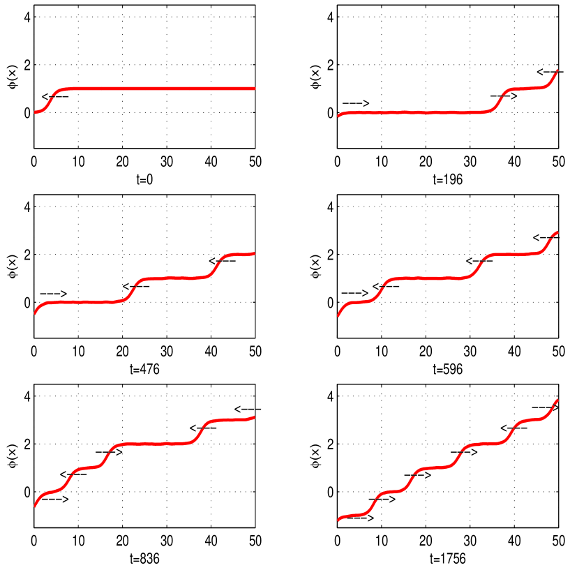
Figure 8: Initial single colliding kink gives rise to configurations with increasingly higher kink number. A sine-Gordon potential (8.1) with $m=1$ and $\lambda=1$ was used. The y-axis is normalised such that the vacuum points correspond to integers. The initial kinetic energy of the single kink is distributed amongst the final kinks that have lower velocity.

Let us illustrate these ideas by looking at the very long time limit of the kink/boundary collision process. Here we will follow [1] and consider a theory with a periodic potential $V(\phi)$. In the situations considered so far the field values were always near the two vaccua $-v$ and $v$, and the large $\phi$ structure of the potential was never relevant. This is not the case, as we will see, for considerably long times after the collision. As we have discussed, when the kink collides with the left boundary some radiation is produced which propagates away in the direction of the opposite right boundary (and vice versa). As the vacuum in the right boundary becomes perturbed, we can expect as before, that the corresponding zero mode becomes excited. From our arguments above this zero mode should with time grow into an additional, left-moving kink. Something similar could be expected to happen in the left boundary, after the reflected kink moves away into the bulk. Since we expect some small perturbation around the vacuum there, another (probably very slow) right-moving kink should start forming. For a periodic potential and very long times this process would repeat itself several times, with increasing numbers of kinks being extracted from both boundaries. That this seems to be indeed the case has been confirmed in Fig. 8. For a sine-Gordon model with potential

$$V(\phi)=-\frac{m^{4}}{\lambda}\left[\cos\left(\frac{\sqrt{\lambda}}{m}\phi\right)-1\right]$$ (8.1)

and parameters $m=1$, $\lambda=1$ we observed the formation of five kinks from an initial single-kink collision. As expected, the kinetic energy of the initial kink is distributed amongst the final kinks that move with much lower velocities.

As an extra test we evolved a number of near vacuum configurations with zero bulk charge and observed the formation of a number of kinks at both boundaries, as expected. The natural question at this point is which mechanism would cause the kink formation process to stop eventually. One possibility is that, as their velocities become increasingly small, a kink gas would form, its density being limited by the repulsive kink-kink interaction. We can conjecture that for a very large family of initial conditions a gas of stacked branes should form, with density closely related to the energy of the initial field configuration. If this happens to be the case, the final charge configuration, in particular the final boundary charges of the system, would be selected by its total energy. Clearly a deeper understanding, both in numerical and analytical terms, of the system is needed in order to clarify these intriguing possibilities.

Acknowledgements
A. L. is supported by a PPARC Advanced Fellowship. N. D. A. is supported by a PPARC Post-Doctoral Fellowship.

References

- [1] N. D. Antunes, E. J. Copeland, M. Hindmarsh and A. Lukas, “Kinky brane worlds,” arXiv:hep-th/0208219.
- [2] A. Lukas, B. A. Ovrut, K. S. Stelle and D. Waldram, “The universe as a domain wall,” Phys. Rev. D 59 (1999) 086001 [hep-th/9803235].
- [3] J. R. Ellis, Z. Lalak, S. Pokorski and W. Pokorski, “Five-dimensional aspects of M-theory dynamics and supersymmetry breaking,” Nucl. Phys. B 540 (1999) 149 [hep-ph/9805377].
- [4] A. Lukas, B. A. Ovrut, K. S. Stelle and D. Waldram, “Heterotic M-theory in five dimensions,” Nucl. Phys. B 552 (1999) 246 [hep-th/9806051].
- [5] A. Lukas, B. A. Ovrut and D. Waldram, “Non-standard embedding and five-branes in heterotic M-theory,” Phys. Rev. D 59 (1999) 106005 [hep-th/9808101].
- [6] M. Brandle and A. Lukas, “Five-branes in heterotic brane-world theories,” Phys. Rev. D 65 (2002) 064024 [arXiv:hep-th/0109173].
- [7] E. Witten, “Small Instantons in String Theory,” Nucl. Phys. B 460 (1996) 541 [hep-th/9511030].
- [8] O. J. Ganor and A. Hanany, “Small Instantons and Tensionless Non-critical Strings,” Nucl. Phys. B 474 (1996) 122 [hep-th/9602120].
- [9] S. Ghoshal and A. B. Zamolodchikov, Int. J. Mod. Phys. A 9, 3841 (1994) [Erratum-ibid. A 9, 4353 (1994)] [arXiv:hep-th/9306002]; S. Ghoshal, Int. J. Mod. Phys. A 9, 4801 (1994) [arXiv:hep-th/9310188]; H. Saleur, S. Skorik and N. P. Warner, Nucl. Phys. B 441, 421 (1995) [arXiv:hep-th/9408004].
- [10] O. DeWolfe, D. Z. Freedman, S. S. Gubser and A. Karch, “Modeling the fifth dimension with scalars and gravity,” Phys. Rev. D 62 (2000) 046008 [hep-th/9909134].
- [11] E. J. Copeland, J. Gray and A. Lukas, “Moving five-branes in low-energy heterotic M-theory,” Phys. Rev. D 64 (2001) 126003 [hep-th/0106285].
- [12] R. Rajaraman, “Solitons and Instantons,” (North-Holland, Amsterdam, 1982).
- [13] W. H. Press, B. P. Flannery, S. A. Teukolsky and W. T. Vetterling, Numerical Recipes in C: The Art of Scientific Computing, (Cambridge University Press, Cambridge, 1990).