hep-th/0310060
FIT HE - 03-04

Gauge-gravity correspondence
in de Sitter braneworld

Kazuo Ghoroku

^†Fukuoka Institute of Technology, Wajiro, Higashi-ku
Fukuoka 811-0295, Japan

We study the braneworld solutions based on a solvable model of 5d gauged supergravity with two scalars of conformal dimension three, which correspond to bilinear operators of fermions in the dual $\mathcal{N}=4$ super Yang-Mills theory on the boundary. An accelerating braneworld solution is obtained when both scalars are taken as the form of deformations of the super Yang-Mills theory and the bulk supersymmetry is completely broken. This solution is smoothly connected to the Poincare invariant brane in the limit of vanishing cosmological constant. The stability of this brane-solution and the correspondence to the gauge theory are addressed.

1 Introduction

It is an important issue to study the correspondence of gravity and gauge theory, especially for the non-conformal case, by extending the original idea of the correspondence between superstring theory on anti-de Sitter space-time (AdS) and conformal field theory (CFT) on the boundary, known as AdS/CFT correspondence [1]. In the extension to the non-conformal case, scalar fields and their potential introduced in the 5d gauged supergravity would play an important role since a non-trivial configuration of these scalars represents a deformation of the CFT or a vacuum expectation value (VEV) of corresponding field operators in CFT (see for a review [2]).

The idea of AdS/CFT has been further extended to the 5d brane-world [18, 19, 20, 21, 23, 22, 24] by considering an ultraviolet cutoff CFT as a dual theory on the brane. In this CFT the cutoff scale is given by the fifth coordinate representing the position of the brane, and wealky coupled gravity appears on the brane. It would be important to extend this idea in various type of braneworld, especially for de Sitter (dS) brane, since it could explain the recent observation of the accelerated expansion of our universe. Up to now any clear gauge/gravity correspondence for dS brane-world has not been given.

We approach to this problem from the brane-world solutions which can be obtained in terms of a bulk action of 5d gauged supergravity. The advantage of this approach is that the scalar fields in this model have definite meaning in the dual theory. Then we can speculate on the gauge/gravity correspondence from these braneworld solutions by assuming the same role of the scalar fields. Secondly, the scalar potential provides the effective cosmological constant for the supersymmetric AdS₅ vacuum.

However, the scalars corresponding to the rellevant operators in CFT are tachyons in the bulk-space. They are allowed in the bulk space since the unitarity bound is satisfied [29]. While they might be trapped as tachyons on the Poincare invariant brane [30]. In this case, the brane solution would be unstable. A possible resolution for this difficulty would be to consider some non-trivial scalar configurations [34] or to take into account of an appropriate coupling of scalars and the brane. Here we study the case where both are considered. The interesting point in the present model is that we can speculate on the gauge/gravity correspondence since the non-trivial solutions of scalars simultaneously represent the deformation or VEV of some operators in the dual gauge theory.

Here we consider the model given in [9] as the bulk action since this is an example of a solvable case. In this model, we study two braneworld solutions with non-trivial scalars, the BPS and non-BPS one. The BPS solution is obtained by solving the first order BPS or supersymmetric conditions [25, 26]. This solution can be connected to the brane by replacing the tension with the superpotential [6, 27], this would be considered as an extended ”Randall-Sundrum fine-tuning condition”. The non-BPS solution is obtained by directry solving the Einstein equations since the BPS conditions are not satisfied. In this case, the brane tension is also replaced by a function of the scalars to satisfy the boundary condition of the solutions. For these solutions, the localization of fields, especially the graviton, the stability, are studied and gravity/gauge theory correspondence is also addressed.

For the BPS case, the brane is Poincare invariant, and discrete massive modes as well as the graviton can be trapped. While for non-BPS (non-supersymmetric) case, we observe the localized graviton and the accelerated expansion of the 3d space on the brane. Namely, we obtain a brane of positive cosmological constant ($\lambda$).

In Section 2, we set our bulk action with two scalars, and brane solutions with BPS condition are shown and discussed in Section 3. Non-BPS solution is given in Section 4 and its stability is shown. In Section 5, the confinement in the dual gauge theories is discussed. In the final section, summary and discussions are given.

2 Bulk action

As a bulk action, consider a model of 5d gauged supergravity given in [9],

$$S_{\rm g}=\int d^{4}\!xdy\sqrt{-g}\left\{{1\over 2\kappa^{2}}R-{1\over 2}\sum_{I}(\partial\phi_{I})^{2}-V(\phi)\right\}\ ,$$ (1)

where the potential $V$ is written by two scalars, $\phi_{1}$ and $\phi_{2}$, as follows,

$$V=-{3\over 8}\left\{(\cosh({2\over\sqrt{3}}\phi_{1}))^{2}+4\cosh({2\over\sqrt{3}}\phi_{1})\cosh({2}\phi_{2})-(\cosh({2}\phi_{2}))^{2}+4\right\}.$$ (2)

We review here the role of scalar fields in this potential from the AdS/CFT viewpoint. $\phi_{1}$ and $\phi_{2}$ are belonging to $\underline{6}$ and $\underline{1}$ respectively in the decomposition $\underline{10}\to\underline{1}+\underline{6}+\underline{3}$ of gauged group $SU(4)$ under $SU(3)\times U(1)$. Their mass is $M^{2}=-3$, and the conformal dimension is $\Delta=3$. They correspond to the mass operators of the chiral superfields and the gaugino of ${\cal N}=4$ SYM. And we expect the same role in the cutoff CFT on the brane.

In this model, the superpotential $W$ is given by

$$W=-{3\over 4}\left(\cosh({2\over\sqrt{3}}\phi_{1})+\cosh({2}\phi_{2})\right),$$ (3)

and $V$ is represented by $W$ as

$$V={v^{2}\over 8}\sum_{I}\left({\partial W\over\partial\phi_{I}}\right)^{2}-{v^{2}\over 3}W^{2},$$ (4)

with a gauge coupling parameter $v$ which is fixed from the AdS₅ vacuum [5]. For $\phi_{1}=\phi_{2}=0$, it is given as $v=\pm 2/L$ in terms of the AdS radius $L$. Here we set as $L=1$ for $\kappa^{2}=2$ as in [9], in which the positive value $v=2/L$ is used. But we take the opposite sign in order to get a positive tension brane as stated below.

The supersymmetric solution for the bulk is obtained under the following ansatz for the metric,

$$ds^{2}=g_{MN}dx^{M}dx^{N}=A^{2}(y)\eta_{\mu\nu}dx^{\mu}dx^{\nu}+dy^{2}\ ,$$ (5)

where $\eta_{\mu\nu}=$diag$(-1,1,1,1)$. In [9], the solution is obtained by solving the following first order equations,

$$\phi_{I}^{\prime}={v\over 2}{\partial W\over\partial\phi_{I}},\qquad{A^{\prime}\over A}=-{v\over 3}W,$$ (6)

where ${}^{\prime}=d/dy$. These equations are known as the necessary conditions for supersymmetry and also for the BPS solutions of a model with scalars [25, 26]. The solutions of (6) satisfy the equations of motion of (1) for any $W$ when we take the 4d slice being Poincare invariant. When we choose the metric of the 4d slice as $A^{2}(y)(-dt^{2}+e^{\sqrt{\lambda}t}\delta_{ij}dx^{i}dx^{j})$ instead of the form of (5), we get the following equation from equation of motion,

$$V={v^{2}\over 8}\sum_{I}\left({\partial W\over\partial\phi_{I}}\right)^{2}-{v^{2}\over 3}W^{2}+{\lambda\over A^{2}}.$$ (7)

This coincides with (4) only if $\lambda=0$.

3 Brane action for BPS solution

Nextly, we consider a brane situated at $y=0$, and this gives the boundary of the bulk space. In this case, the field equations include the $\delta$-function parts, which give the boundary conditions for the bulk solutions considered in the previous section. They are the conditions for $\phi_{I}^{\prime}(0)$ and $A^{\prime}(0)/A(0)$ to cancel the $\delta$-function term in each equations.

It is possible to take the boundary conditions such that we can preserve the the form of the supersymmetric or BPS bulk solutions by an appropriate choice of the brane action which depends on the bulk scalar fields. The most simple form is obtained as follows [6, 27],

$$S_{\rm br}=-v\int d^{4}\!x\sqrt{-\det g_{\mu\nu}}~{}W\ .$$ (8)

While, we notice that the action

$$S=S_{\rm g}+S_{\rm br}$$

does not guarantee the supersymmetry of the model. Actually, we would need other terms and fields for the supersymmetry as shown in [6] for $\mathcal{N}=2$ gauged supergravity. However it would be possible to consider this action as on shell supersymmetric form as in the $\mathcal{N}=2$ case [27]. Then, we consider this action is enough to solve the classical equations of motion. So other necessary terms and fields for the supersymmetry are not considered here since they are not needed in the following discussions. In this sense, our model might be incomplete from the viewpoint of supergravity.

3.1 BPS solution

We consider the brane of positive tension. Since $W$ is negative, we should take negative $v(=-2/L)$ to obtain the brane of positive tension. The solution is obtained under the metric given in (5). Since the boundary conditions are automatically satisfied by the solutions of (6) due to the brane action (8), it is easy to obtain the following solution,

$$A=A_{0}\sinh^{1/2}(y_{H}-|y|)\sinh^{1/6}[3(y_{H^{\prime}}-|y|)]$$ (9)

$$\phi_{1}={\sqrt{3}\over 2}\ln\coth[(y_{H}-|y|)/2]\ ,\qquad\phi_{2}={1\over 2}\ln\coth[3(y_{H^{\prime}}-|y|)/2]$$ (10)

Here we consider the case of $y_{H}<y_{H^{\prime}}$ as in [9]. And we set as $A(0)=1$, then $A_{0}=\sinh^{-1/2}(y_{H})\sinh^{-1/6}(3y_{H^{\prime}})$. The solution is taken to be $Z_{2}$ symmetric, the symmetry under the transformation $y\to-y$.

From the viewpoint of the boundary field theory, we expect that the solution $\phi_{1}$ gives a deformation of ${\cal N}=4$ SYM, and it corresponds to the mass of three chiral superfield of ${\cal N}=4$ SYM. While $\phi_{2}$ represents the VEV of gaugino and it specifies a different phase of the same ${\cal N}=1$ SYM theory. And these provides a RG flow of the theory from ${\cal N}=4$ SYM to the ${\cal N}=1$ SYM in the infrared limit as discussed in [9]. It would be interesting point to see these correspondence from the boundary field theory which include gravity in the present case.

This solution might be supersymmetric, at least in the bulk, but a singularity is found at the horizon $y=y_{H}(<y_{H^{\prime}})$ where scalar curvature diverges. Some corrections from superstring theory might be needed near this region to resolve this singularity. While it would be meaningful to see various features of this solution as a brane-world in the range $0<y<y_{H}$ as in the case of de Sitter brane, where the similar horizon appears.

3.2 Gravity localization

When we consider a brane-world, the most important point is the localization of the gravity or the trapping of the zero mode of 5d graviton. We study this point for the present solution. The field equation of the graviton is obtained as follows. Consider the 4d part of the metric-fluctuation, $h_{\mu\nu}$, around the flat background as,

$$ds^{2}=A^{2}(y)[\eta_{\mu\nu}+h_{\mu\nu}(x^{\mu},y)]dx^{\mu}dx^{\nu}+dy^{2}\,.$$ (11)

Then the transverse and traceless part $h$ is projected out by $\partial_{\mu}h^{\mu\nu}=0$ and $h^{\mu}_{\mu}=0$. In this case, one arrives at the following linearized equation of $h$ in terms of the five dimensional covariant derivative $\nabla^{2}_{5}=\nabla_{M}\nabla^{M}$:

$$\nabla^{2}_{5}h=0.$$ (12)

This is equivalent to the field equation of a five dimensional free scalar. Eq. (12) is written by expanding $h$ in terms of the four-dimensional continuous mass eigenstates:

$$h=\int dm\phi_{m}(t,x^{i})\Phi(m,y)\,,$$ (13)

where the 4d mass $m$ is defined by the 4d laplacian $\nabla^{2}_{4}$ as

$$\nabla^{2}_{4}\phi_{m}=m^{2}\phi_{m}\,.$$ (14)

The equation for $\Phi(m,y)$ is obtained as

$${\Phi}^{\prime\prime}+4{A^{\prime}\over A}{\Phi}^{\prime}+{m^{2}\over A^{2}}\Phi=0.$$ (15)

Introducing $u(z)$ and $z$ defined as $\Phi=A^{-3/2}u(z)$ and $\partial z/\partial y=\pm A^{-1}$, Eq.(15) can be rewritten into the Schrödinger-like equation as,

$$[-\partial_{z}^{2}+V_{S}(z)]u(z)=m^{2}u(z),\$$ (16)

where $V_{S}(z)$ is expressed by $A(y)$ or $\tilde{A}(z)=\ln A(y)$ as

$$V_{S}(z)={9\over 4}(A^{\prime})^{2}+{3\over 2}AA^{\prime\prime}={9\over 4}(\partial_{z}\tilde{A})^{2}+{3\over 2}\partial_{z}^{2}\tilde{A}.$$ (17)

We notice prime denotes still derivative with respect to $y$, namely ${}^{\prime}=d/dy$ (not $d/dz$). In the latter of (17), $z$-derivative and $\tilde{A}$ are used. The latter form is usually seen in the literature. The problem of localization is solved by this one-dimensional Schrödinger-like equation (16) for the states of 4d mass-eigenvalue $m^{2}$. The potential $V_{S}(z)$ in Eq. (16) is determined by $A(y)$.

Before considering the solution of Eq. (16), we note that this equation can be written in a ”supersymmetric” form as

$$Q^{\dagger}Qu(z)=(-\partial_{z}-{3\over 2A}{\partial A\over\partial z})(\partial_{z}-{3\over 2A}{\partial A\over\partial z})u(z)=m^{2}u(z).$$ (18)

So the eigenvalue $m^{2}$ should be non-negative, i.e., no tachyon in four dimension. Then the zero mode $m=0$ is the lowest state which might be localized on the brane. Next, we see the behavior of the potential $V_{S}$. Although the new variable can be obtained through the integration $z=\int dy/A(y)$ explicitly, this is complicated for the present solution, so we see the potential $V_{S}$ in y-space. Then it is expressed as

$$V_{S}={3\over 4}{\sinh(y_{H}-y)\sinh^{1/3}(3(y_{H^{\prime}}-y))\over\sinh(y_{H})\sinh^{1/3}(3y_{H^{\prime}})}\left\{{5\over 4}\left(\coth(y_{H}-y)+\coth(3(y_{H^{\prime}}-y))\right)^{2}\right.$$

$$\left.-\left({1\over\sinh^{2}(y_{H}-y)}+{3\over\sinh^{2}(3(y_{H^{\prime}}-y))}\right)\right\}+2W\delta(y),$$ (19)

We notice that this potential is singular at the position of the brane, $y=0$, due to the $\delta$-function. And $V_{S}$ is also singular at $y=y_{H}$. Its typical behavior is shown in Fig.1. The singular behavior $V_{S}(y_{H})=+\infty$ is not changed when we take $y_{H}\leq y_{H^{\prime}}$. Then we must impose following two boundary conditions for $u(z)$,

$$u(z_{H})=0,\quad{u^{\prime}(z_{0})\over u(z_{0})}=W(\phi_{I}(0))$$ (20)

where $z_{0}$ ($z_{H}$) denotes the value of $z$ at $y=0$ ($y=y_{H}$).

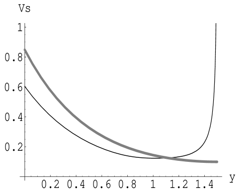
Fig. 1: The potential in the Schrödinger type equation, $V_{S}(y)={9\over 4}(A^{\prime})^{2}+{3\over 2}AA^{\prime\prime}$, for $y_{H}=1.5$ are shown. The solid curve represents the one for $\mathcal{N}=1$ supersymmetric and gaugino condensed, and the thick, gray curve is for non-supersymmetric solution. The normalization is free.

These two conditions are written in terms of $\Phi(y)$ as

$$\Phi^{\prime}(0)=0,~{}~{}~{}\Phi(y_{H}-\epsilon)=O\left(\epsilon^{\alpha}\right),\quad\alpha>-{3\over 4}.$$ (21)

The first condition is obvious from Eq.(15), and the second one is obtained from $\Phi=A^{-3/2}u(z)$. Using this representation, we consider the zero mode denoted by $\Phi_{0}(y)$. From (15), $\Phi_{0}(y)$ is obtained as

$$\Phi_{0}^{\prime}(y)={c_{0}\over A^{4}(y)},$$ (22)

where $c_{0}$ is an integration constant. Then we find $c_{0}=0$ from the first equation of (21) since $A(0)=1$. Then $\Phi_{0}(y)=$ constant, and it satisfies the second Eq. of (21). This result implies that the graviton can be trapped on the brane in the supersymmetric background. In this case, many discrete massive modes might be also trapped due to the special form of the potential.

From the viewpoint of gauge/gravity correspondence, the massive state satisfying the two boundary conditions would be a tensor state constructed as a composite of the fields of SYM theory. This point is assured from the the fact that the gauge theory on the brane is in a confinement phase as seen from the analysis of the Wilson-loop as shown below. It is out of the present work to study the spectrum of these bound states, so we do not discuss on this point furthermore.

We can easily obtain the solution of $\phi_{2}=0$ or without the gaugino condensation, and we find the similar properties with the present solution. It is abbreviated here for the simplicity, but we can say that the graviton can be trapped on the brane for the supersymmetric solutions.

4 Non-BPS braneworld solution

From the bulk action $S_{\rm g}$ in (1), it is possible to obtain a more favorite brane-world solution under the following ansatz,

$$\phi\equiv{2\over\sqrt{3}}\phi_{1}=2\phi_{2}\,.$$ (23)

However this ansatz can not satisfy the first equations of (6) for the given $W$, so the solution breaks the supersymmetry or the BPS condition in this case. Then we can’t use the first order equations (6), and we must solve directly the equations of motion of the second order. Further, the brane action should be changed from $W$ to a generalized form $F(\phi)$ as

$$S_{\rm br}^{\rm ge}=-\tau\int d^{4}\!x\sqrt{-\det g_{\mu\nu}}F(\phi_{I})\ ,$$ (24)

where $\tau$ denotes the brane tension, and $F(\phi_{I})$ represents the scalar-brane coupling, and its explicit form is not necessary here. Secondly, we take the following new ansatz for the metric,

$$ds^{2}=g_{MN}dx^{M}dx^{N}=A^{2}(y)(-dt^{2}+a^{2}(t)\gamma_{ij}dx^{i}dx^{j})+dy^{2}\ ,$$ (25)

where $\gamma_{ij}=(1+k\delta_{mn}x^{m}x^{n}/4)^{-2}\delta_{ij}$. As long as we do not mention, $k=0$ and $a_{0}=e^{\sqrt{\lambda}t}$, where $\lambda$ is the 4d cosmological constant.

Then, we set the following action

$$S=S_{\rm g}+S_{\rm br}^{\rm ge},$$

and the equations of motion are given as

$$G_{MN}=\kappa^{2}\left\{\sum_{I}\partial_{M}\phi_{I}\partial_{N}\phi_{I}-g_{MN}\left({1\over 2}\sum_{I}(\partial\phi_{I})^{2}+V\right)-g_{\mu\nu}\delta_{M}^{\mu}\delta_{N}^{\nu}\tau F(\phi_{I})\delta(y)\right\}\ ,~{}~{}~{}$$ (26)

$$\qquad\qquad{1\over\sqrt{-g}}\partial_{M}\left\{\sqrt{-g}g^{MN}\partial_{N}\phi_{I}\right\}={\partial V\over\partial\phi_{I}}+{\sqrt{-\det g_{\mu\nu}}\over\sqrt{-g}}~{}\tau{\partial F\over\partial\phi_{I}}\delta(y)\ .$$ (27)

Here we solve these under the following ansatz for metric, When we take as $\phi=\phi(y)$, (26) and (27) are written as

$${A^{\prime\prime}\over A}+\left({A^{\prime}\over A}\right)^{2}-{\lambda\over A^{2}}=-{\kappa^{2}\over 3}\left({1\over 2}\sum_{I}(\phi^{\prime}_{I})^{2}+V(\phi)\right)-{\kappa^{2}\tau\over 3}F(\phi_{I})\delta(y)\ ,$$ (28)

$$\qquad\qquad\left({A^{\prime}\over A}\right)^{2}-{\lambda\over A^{2}}={\kappa^{2}\over 6}\left({1\over 2}\sum_{I}(\phi^{\prime}_{I})^{2}-V(\phi)\right)\ ,$$ (29)

$$\qquad\qquad\phi^{\prime\prime}_{I}+4\phi^{\prime}_{I}{A^{\prime}\over A}={\partial V\over\partial\phi_{I}}+\tau{\partial F\over\partial\phi_{I}}\delta(y)\ ,$$ (30)

where ${}^{\prime}=d/dy$.

Then we find the following solution

$$A(y)=\sqrt{3\lambda}\sinh(y_{H}-|y|)\ ,\quad\phi(y)=\ln\left(\coth\left({y_{H}-|y|\over 2}\right)\right),$$ (31)

where $\lambda$ is positive and arbitrary. And we need the following boundary conditions,

$${A^{\prime}(0)\over A(0)}=-{\kappa^{2}\tau\over 6}F(\phi_{I}(0))~{},$$ (32)

$$\phi^{\prime}(0)={\tau}{\partial F(\phi(0))\over\partial\phi_{2}}~{},\qquad{1\over\sqrt{3}}{\partial F(\phi(0))\over\partial\phi_{1}}={\partial F(\phi(0))\over\partial\phi_{2}}~{}.$$ (33)

Several comments are given for this solution. Here we could introduce the bulk cosmological constant, $\Lambda=0$, since the supersymmetry is not preserved here. But we obtain $\Lambda=0$ as a result even if it is introduced. The reason of this result is in a special form of the scalar potential, which is consistent with supersymmetry. In this sense, this result is considered as a remnant of the supersymmetry. However an arbitrary and positive value of $\lambda$ is allowed, and the four dimensional part of the metric is given as

$$ds_{4}^{2}=-dt^{2}+e^{\sqrt{\lambda}~{}t}~{}\delta_{ij}dx^{i}dx^{j}.$$ (34)

This is the inflation universe with a positive cosmological constant, and this is the consequence of supersymmetry breaking. Due to the ansatz (23), both scalars are the deformations of SYM and they represent the mass operators of three chiral super-fields and the gaugino in the SYM. Then the supersymmetry of SYM on the brane is completely broken in the present case. So the explicit form of $\phi(y)$ represents the RG flow of the fermion mass. Its value at $y=0$ is given as $\phi(0)\sim\sqrt{3\lambda}$ at small $\lambda$, and this vanishes for $\lambda=0$ as expected.

Next, we notice that this solution has the same form with the one obtained previously for negative $\Lambda$ without scalars [35] and with a scalar [34]. The present solution is easily identified with the one of [34] by adjusting the parameters as, $\alpha=\sqrt{\lambda}$ and $\mu=1$.

Then the localization of the fields can be assured in a parallel way, and we can say that the gravity and also gauge bosons [34, 36] are localized on this brane. As for the localization of scalar fields introduced here, we discuss in the following sub-section.

4.1 Fluctuations and stability of the solution

We must investigate the fluctuations of the scalar fields to see the stability of the solution since the fluctuations might be tachyonic in general. If these tachyonic modes were trapped on the brane as tachyons then the brane would be unstable. The situation is a little complicated when the configuration of scalars are non-trivial since their fluctuations mix with scalar component of metric fluctuations. The latter are the unphysical degrees of freedom when we consider the pure gravity, so they should not affect on any physical result. But the situation is changed when they mix with the physical scalar modes. So we must solve the coupled equations to see their spectrum and the localization in this case.

In the present case, there are two scalar-freedoms. Firstly, we solve the one mixed with the metric fluctuations. The discussion for this problem is parallel to the case given in [34] for one scalar. In order to simplify the equations, change the coordinate from $y$ to $z$ in terms of the relation, $dy/dz=A(y)$, then the metric is rewritten as

$$ds^{2}=g_{MN}dx^{M}dx^{N}=A^{2}(z)(\gamma_{\mu\nu}dx^{\mu}dx^{\nu}+dz^{2})\ ,$$ (35)

where $\gamma_{\mu\nu}dx^{\mu}dx^{\nu}=(-dt^{2}+a^{2}(t)\gamma_{ij}dx^{i}dx^{j})$. And fluctuations of scalar and metric are introduced as follows,

$$\phi_{I}=\bar{\phi}_{I}+\delta\phi_{I}$$

$$ds^{2} = A^{2}(z)\big{[}\left((1+2\psi)\gamma_{\mu\nu}+2h_{\mu\nu}+(\nabla_{\mu}f_{\nu}+\nabla_{\nu}f_{\mu})+2\nabla_{\mu}\nabla_{\nu}E\right)dx^{\mu}dx^{\nu}$$

$$+ (B_{\mu}+2\nabla_{\mu}C)dzdx^{\mu}+(1+2\xi)dz^{2}\big{]}.$$ (36)

Here $\bar{\phi}_{I}$ denote the solution of scalars, $\bar{\phi}_{1}=\sqrt{3}\phi/2$ and $\bar{\phi}_{2}=\phi/2$, and $\nabla_{\mu}$ represents the covariant derivative with respect to $\gamma_{\mu\nu}$.

Here we take the longitudinal gauge ($C=E=f_{\mu}=0$), then the scalar part is written as

$$ds^{2}=A^{2}(z)\left[(1+2\xi)dz^{2}+(1+2\psi)\gamma_{\mu\nu}dx^{\mu}dx^{\nu}\right].$$ (37)

Then the following equations for the scalar components are obtained,

$$3\nabla^{2}\psi+12\mathcal{H}\partial_{z}\psi-12\mathcal{H}^{2}\xi+12\lambda\psi=\sum_{I}\left(\partial_{z}\bar{\phi}_{I}\delta\partial_{z}\phi_{I}-\xi(\partial_{z}\bar{\phi}_{I})^{2}-A^{2}\frac{\partial V}{\partial\bar{\phi}_{I}}\delta\phi_{I}\right),$$ (38)

$$-3\nabla_{\mu}\partial_{z}\psi+3\mathcal{H}\nabla_{\mu}\xi=\sum_{I}\partial_{z}\bar{\phi}_{I}\nabla_{\mu}\delta\phi_{I},$$ (39)

$$\Big{(}3\partial_{z}^{2}\psi-6\xi\partial_{z}\mathcal{H}-3\mathcal{H}\partial_{z}\xi+9\mathcal{H}\partial_{z}\psi-6\mathcal{H}^{2}\xi+\nabla^{2}\xi+2\nabla^{2}\psi+6\lambda\psi\Big{)}\gamma_{\mu\nu}$$

$$\hskip 28.45274pt-\nabla^{2}\xi-2\nabla^{2}\psi=\sum_{I}\left(-\partial_{z}\bar{\phi}_{I}\partial_{z}\delta\phi_{I}+\xi(\partial_{z}\bar{\phi}_{I})^{2}-A^{2}\frac{\partial V}{\partial\bar{\phi}_{I}}\delta\phi_{I}\right)\gamma_{\mu\nu},$$ (40)

and for scalars,

$$\partial_{z}^{2}\delta\phi_{I}+3\mathcal{H}\partial_{z}\delta\phi_{I}+(4\partial_{z}\psi-\partial_{z}\xi-6\mathcal{H}\xi)\partial_{z}\bar{\phi}_{I}-2\xi\partial_{z}^{2}\bar{\phi_{I}}+\nabla^{2}\delta\phi_{I}$$

$$~{}~{}~{}~{}~{}~{}~{}~{}~{}~{}~{}~{}~{}~{}~{}=A^{2}\left(\sum_{J}\frac{\partial^{2}V}{\partial\bar{\phi}_{I}\partial\bar{\phi}_{J}}\delta\phi_{J}+\tau{\partial^{2}F\over\partial\phi_{I}^{2}}\delta\phi_{I}\delta(y)\right),$$ (41)

where $\mathcal{H}=\partial_{z}A/A$ and $\nabla^{2}=\gamma^{\mu\nu}\nabla_{\mu}\nabla_{\nu}$.

The equation for $\psi$ is obtained as follows. From (39), we obtain

$$\sum_{I}\partial_{z}\bar{\phi}_{I}\delta\phi_{I}={1\over 2}\partial_{z}\phi(\sqrt{3}\delta\phi_{1}+\delta\phi_{2})=\left(-3\partial_{z}\psi+3\mathcal{H}\xi\right),$$ (42)

and from the off-diagonal part of eq.(40), we get

$$\xi+2\psi=0.$$ (43)

Substituting these (42) and (43) into Eq.(38)$+$(40), and noticing $\partial_{z}^{2}\bar{\phi}_{I}/\partial_{z}\bar{\phi}_{I}=0$ for our solution, we find

$$-\partial_{z}^{2}{\psi}-3\mathcal{H}\partial_{z}{\psi}-\left(4\partial_{z}{\mathcal{H}}+6\lambda\right)\psi=\nabla^{2}\psi\,.$$ (44)

In deriving this equation, the classical equations are used.

Then, $\psi$ is decomposed as follows in terms of the four-dimensional continuous mass eigenstates:

$$\psi=\int\!dm\ \varphi_{1}^{m}(t,x^{i})\,\Phi_{1}(m,y)\,,$$ (45)

where the 4d mass $m$ is defined by $\nabla^{2}\varphi_{1}^{m}=m^{2}\varphi_{1}^{m}$. In order to see the localization, the explicit form of $\varphi_{m}$ is not necessary, and we need only the exact form of $\Phi_{1}(m,y)$. Its equation is rewritten into the one-dimensional Schrödinger-like equation with the rescaled $\Phi_{1}(m,y)$ as $\Phi_{1}(m,y)=A^{-3/2}u_{1}(z)$ and modified eigenvalue $\tilde{m}^{2}$,

$$[-\partial_{z}^{2}+V_{1}(z)]u_{1}(z)=\tilde{m}^{2}u_{1}(z),\$$ (46)

where $\tilde{m}^{2}=m^{2}+6{\lambda}$ and $V_{1}(z)={9\over 4}(\partial_{z}\tilde{A})^{2}-{5\over 2}\partial_{z}^{2}\tilde{A}={9\over 4}(A^{\prime})^{2}-{5\over 2}AA^{\prime\prime}.$Here we must notice that ^′ denotes $d/dy$ and $\tilde{A}=\ln A$ as in the previous sections. For the present solution, $z=(3\lambda)^{-1/2}\ln(\coth[(y_{H}-|y|)/2])$ and

$$V_{1}(z)={3}\lambda\left({9\over 4}+{1\over\sinh^{2}(\sqrt{3\lambda}z)}\right)+5\sqrt{1+3\lambda}~{}\delta(|z|-z_{0})$$ (47)

The second $\delta$-function term comes from $A^{\prime\prime}$ since it is written in a $Z_{2}$ symmetric form. Then $u$ must satisfy the following boundary condition at $z=z_{0}$,

$$\partial_{z}u_{1}(z_{0})={5\over 2}\sqrt{1+3\lambda}~{}u_{1}(z_{0}).$$ (48)

The eigenvalue $\tilde{m}^{2}$ of the bound state is given by solving the above equation (48). But we should notice that $m^{2}$ might be negative for small $\tilde{m}^{2}$ even if the eigenvalue $\tilde{m}^{2}$ was positive.

As is well known, however, the positive $\delta$-function potential at the brane position, means a strong repulsion for scalar and graviton. Then we can not expect a localized state for any value of $\tilde{m}^{2}$. Actually we can see that there is no bound state, which satisfies (48), in terms of explicit form of $u_{1}(z)$. The general solution of (46) is written by two independent hyper geometric functions ${}_{2}F_{1}$. When $\tilde{m}^{2}$ is larger than the minimum of the analytic part of $V_{1}(z)$, i. e. for $\tilde{m}^{2}>27\lambda/4$, we find oscillating solutions of continuum KK mode. For $\tilde{m}^{2}<27\lambda/4$, there might be a trapped state and its normalizable wave function can be written by one of the hyper geometric functions. Using this wave function, we can show $\partial_{z}u_{1}(0)<{5\over 2}\sqrt{1+3\lambda}u_{1}(z_{0})$ for any $m^{2}$. So there is no solution of Eq.(48) for the trapped state. Then any mode of $\psi,\xi$ and the combination of scalars $\sqrt{3}\delta\phi_{1}+\delta\phi_{2}$, which is mixed with $\psi$ and $\xi$, are not trapped on the present brane even if they were tachyonic in the bulk space. In this sense, the brane is stable for these fluctuations.

Next, we see another scalar-freedom which is represented by a combination of the two scalar fluctuations decoupled to the metric fluctuations. It is given by $\delta\phi=\delta\phi_{1}-\sqrt{3}\delta\phi_{2}$, and its equation is obtained from (41) as

$$\partial_{z}^{2}{\delta\phi}+3\mathcal{H}\partial_{z}{\delta\phi}+\nabla^{2}\delta\phi=\left\{A^{2}\left(2\sinh^{2}(\phi)4-3\right)+{\tau\over 4}\left({\partial^{2}F\over\partial\phi_{1}^{2}}+3{\partial^{2}F\over\partial\phi_{2}^{2}}\right)\delta(y)\right\}\delta\phi\,.$$ (49)

And as above, it is rewritten in the Schrödinger form,

$$[-\partial_{z}^{2}+V_{2}]u_{2}(z)={m}^{2}u_{2}(z) V_{2}(z)={9\lambda\over 4}\left({17\over 3}+{1\over\sinh^{2}(\sqrt{3\lambda}z)}\right)+w_{2}\delta(|z|-z_{0})~{},$$ ,

$$w_{2}=-3\sqrt{1+3\lambda} + {\tau\over 4}\left({\partial^{2}F\over\partial\phi_{1}^{2}}+3{\partial^{2}F\over\partial\phi_{2}^{2}}\right).$$ (50)

In this case, the boundary condition for $u_{2}(z)$ is given as

$${\partial_{z}u_{2}(z_{0})}={w_{2}\over 2}~{}u_{2}(z_{0}),~{}$$ (51)

Then, from $V_{2}(z)$, the wave function for the normalizable bound state in this case should be searched for ${m}^{2}<51\lambda/4$. The solution can be expressed by a hypergeometric function, which is abbreviated here for simplicity. The important point is that the coefficient, $w_{2}$, of the $\delta$-function in the potential $V_{2}$ consists of two parts as shown in the third equation of (50).

When the second positive term is negligible small compared to the negative first term, then $w_{2}$ is negative and we could find a bound state of negative $m^{2}$. Actually, we find a tachyonic bound state for $w<-1.8$ and $\lambda=0.1$. So the brane solution is unstable in this case.

While $w_{2}$ becomes positive when the second term is large enough, or the scalar-brane couplings are strong. In this case, the brane becomes stable because any mode of $m^{2}$ can not be trapped on the brane by the same reason with the first case of the scalar fluctuation which is mixed with metric fluctuations. This stability is always realized by choosing appropriate forms of $F_{I}(\phi_{I})$. In this sense, we can obtain a stable de Sitter brane by breaking the sypersymmetry.

5 Confinement

Here we examined two kinds of brane solutions. One is the BPS solution, which might be supersymmetric, and the non-BPS one. The AdS vacuum solution is included in the latter solution as the limit of $\lambda=0$ since this limit is realized by $y_{H}\to\infty$ or $\phi=0$. For non-BPS case, the potential in the Schrödinger-like equation is regular at the horizon $y_{H}$. And the spectrum of the KK modes is continuous although there is a gap. While the potential is singular at the horizon in cases of supersymmetric solutions with non-trivial scalars. As a result, we could observe the graviton and extra KK discrete modes on the brane as trapped spectra.

From the viewpoint of gauge/gravity correspondence, this discrete eigenvalue would represent the glueball mass. It is straightforward to estimate the mass, but we do not do it here and show them elsewhere. In other words, the quark confinement is implied in this case for the boundary gauge theory. While the gauge theory dual to the non-BPS brane solution is not in the confining phase, so the extra discrete massive modes are not trapped in this case.

This point is also examined in terms of the Wilson loop. According to [3, 9], the Wilson loop of time interval $T$ is expressed by the following action

$$S_{\rm W}=\int dtd\sigma\sqrt{-G_{\rm ind}}=T\int dx\rho(y)A(y)\sqrt{(\partial_{x}y)^{2}+A^{2}(y)}$$ (52)

where we approximated such that $a_{0}(t)=e^{\sqrt{\lambda}t}\sim 1$ for non-supersymmetric solution since the time interval, $T$, of the Wilson loop is considered to be very small compared to $1/\sqrt{\lambda}$, which represents the scale of the universe. The tension of fundamental (F) or Dirichlet (D) string is denoted by an abbreviated notation $\rho(y)$, and they are given as [9],

$$\rho_{F}=4\left\{\cosh{4\phi_{1}\over\sqrt{3}}+\cosh\left({2\phi_{1}\over\sqrt{3}}+2\phi_{2}\right)\right\},\quad\rho_{D}=8\left(\cosh\left({\phi_{1}\over\sqrt{3}}-\phi_{2}\right)\right)^{2}~{}.$$ (53)

Then the quark-antiquark or monopole-antimonopole energy, $S_{\rm W}/T$, is represented as

$${\cal E}=\int dx\sqrt{(\partial_{x}u)^{2}+f(u)},\quad f(u)=\rho^{2}(y)A^{4}(y),$$ (54)

where $u$ is defined by $\partial_{y}u=\rho(y)A(y)$. For non-trivial supersymmetric solutions, the behavior of function $f(u)$ near the horizon, $u\sim u_{H}$, are given [9] as

$$f_{F1}\sim 1,\quad f_{D1}\sim|u-u_{H}|.$$ (55)

This implies quark confinement and monopole screening. As for the non-supersymmetric solution, we obtain

$$f_{F1}\sim|u-u_{H}|^{2},\quad f_{D1}\sim|u-u_{H}|^{4}.$$ (56)

The potential for monopole is expected to be $1/r$ Coulomb type, and quark is not confined but in a screening phase. The latter result is consistent with the discussion given above for the gluon spectrum.

There may be another solution of confinement phase even if all fermions get mass and all supersymmetries are broken [15]. In this solution $\lambda=0$, then it is different from our solution.

6 Summary

Here, we examined brane solutions based on a five dimensional gauged supergravity with two scalar fields. From the holographic viewpoint, these scalars correspond to the fermion mass operators of three chiral super-fields and gaugino in $\mathcal{N}=4$ SYM theory. The solutions of this model are interpreted as the renormalization group flow of the dual gauge theories on the boundary. This interpretation might be also available for the braneworld solutions by considering a dual 4d field theory on the brane with an ultraviolet cut-off.

We obtained two types of solutions, BPS solution, which might be supersymmetric, and non-BPS one, with non-trivial scalar configurations. For BPS case, the 4d slice is Poincare invariant. Then the cosmological constant is zero, $\lambda=0$, and the gravity as well as discrete massive modes are trapped. As a result, we can assure the quark confinement and the discrete glueball mass for this case. This property is supported by the infrared singularity of the potential in the Schrödinger-like field equation near the horizon. This singularity disappears in the case of AdS vacuum solution, and quark confinement property disappears because of the restored conformal symmetry.

For non-BPS case, we obtain a de Sitter brane solution with $\lambda>0$. This result is considered as the complete supersymmetry breaking. Actually, the scalars are in this case interpreted as deformations of CFT and all fermions in CFT becomes massive as a result. This is consistent with the result of no supersymmetry. While in this case, we can consider this brane as a candidate of our universe due to the positive $\lambda$. Further, we can show that the solution is stable against the scalar fluctuations since the probable tachyonic modes can not be trapped due to the mixing with the fluctuations of scalar components of the metric and by imposing a strong coupling with brane. In this background, the KK modes of free scalar has a continuous spectra with a mass gap, and there is no discrete bound state. This implies the quark non-confinement in the dual gauge theory. This is reduced to the non-existence of singularity near the horizon in the potential of Schrödinger-like field equation. We can assure this non-confinement also through the analysis of the Wilson loop.

Here the scalars are restricted to a small number and a special case, but it would be expected that more scalars might be needed to get a more realistic brane-world. Then it would be meaningful to make analysis in terms of another kinds of scalars based on the same five dimensional $\mathcal{N}=8$ gauged supergravity to understand more deeply the correspondence of gauge theory and gravity.

References

- [1] J. M. Maldacena, Adv. Theor. Math. Phys. 2, 231 (1998) (hep-th/9711200). S. S. Gubser, I. R. Klebanov and A. M. Polyakov, Phys. Lett. B 428, 105 (1998) (hep-th/9802109). E. Witten, Adv. Theor. Math. Phys. 2, 253 (1998) (hep-th/9802150). A.M. Polyakov, Int. J. Mod. Phys. A14 (1999) 645, (hep-th/9809057).
- [2] F.Bigazzi, A.L. Cotrone, M. Petrini, and A. Zaffaroni, Riv. Nuovo Cim. 25N12 (2002) 1-70, (hep-th/0303191).
- [3] L. Girardello, M. Petrini, M. Porrati and A. Zaffaroni, JHEP 9812 (1998) 022 (hep-th/9810126); JHEP 9905 (1999) 026 (hep-th/9903026).
- [4] J. Distler and F. Zamora, Adv. Theor. Math. Phys. 2 (1998) 1405, (hep-th/9810206).
- [5] D. Freedman, S. Gubser, K. Pilch, and N. Warner, Adv. Theor. Math. Phys. 3, 363 (1999) (hep-th/9904017).
- [6] E. Bergshoeff, R. Kallosh and A. Van Proeyen, JHEP 0010 (2000) 033, (hep-th/0007044).
- [7] A. Khavaev, K. Pilch and N.P. Warner, Phys. Lett. B487 (2000) 14.
- [8] A. Karch, D. Lüst and A. Miemiec, Phys. Lett B454 (1999) 265; (hep-th/9810254).
- [9] L. Girardello, M. Petrini, M. Porrati and A. Zaffaroni, Nucl. Phys. B 596, 451 (2000) (hep-th/9909047).
- [10] D.Z. Freedman, S.S. Gubser, K. Pilch and N.P. Warner, JHEP 0007 (2000) 03, (hep-th/9906194).
- [11] K. Pilch and N.P. Warner, Phys. Lett. B487 (2000) 22, (hep-th/0002192); Nucl. Phys. B594 (2001) 209; (hep-th/0004063).
- [12] S.S. Gubser, Adv. Theor. Math. Phys. 4 (2002) 679, (hep-th/0002160).
- [13] A. Brandhuber and K. Sfetsos, Phys. Lett. B488 (2000) 373; (hep-th/0004148).
- [14] N. Evans and M. Petrini, Nucl. Phys. B592 (2001) 129; (hep-th/0006048).
- [15] J. Babington, D.E. Crooks and N. Evans, (hep-th/0207076); (hep-th/0210068).
- [16] S. Nojiri and S.D. Odintsov, Phys. Lett. B449 (1999) 39, (hep-th/9812017); Phys. Lett. B458 (1999) 226, (hep-th/9904036).
- [17] A. Buchel, Phys.Rev. D65 (2002) 125015, (hep-th/0203041); Phys. Lett. B570 (2003) 89, (hep-th/0302107).
- [18] H. Verlinde, Nucl. Phys. B580 (2000) 264; hep-th/9906182.
- [19] N. Arkani-Hamed, M. Porrati and L. Landall, JHEP 0108 (2001) 021, (hep-th/0012148).
- [20] R. Rattazzi and A. Zaffaroni, JHEP 0104 (2001) 017 (hep-th/0012248).
- [21] S.B. Giddings, E. Katz and L. Randall, JHEP 03 (2000) 023, (hep-th/0009176).
- [22] M.J. Duff and J. T. Liu, Phys. Rev. Lett. 85 (2000) 2052, (hep-th/0003237).
- [23] M. Perez-Victoria, JHEP 0105 (2001) 064 (hep-th/0105048).
- [24] K. Ghoroku, and M. Yahiro, Phys. Rev. 66 (2002) 124020, (hep-th/0206128).
- [25] K. Skenderis and P.K. Townsend, Phys. Lett. B468 (1999) 46, (hep-th/9909070).
- [26] O. DeWolfe, D. Freedman, S. Gubser, and A. Karch, Phys. Rev. D62, 046008 (2000) (hep-th/9909134).
- [27] Ph. Brax and A.C. Davis, Phys. Lett. B447 (2001) 289, (hep-th/0011045).
- [28] L. Randall and R. Sundrum, Phys. Rev. Lett. 83, 4690 (1999), (hep-th/9906064); Phys. Rev. Lett. 83, 3370 (1999), (hep-ph/9905221).
- [29] P. Breitenlohner and D.Z. Freedman, Ann. Phys. 144 (1982) 249; Phys. Lett. B115 (1982) 197.
- [30] K. Ghoroku, and A. Nakamura, Phys. Rev. D64 (2001) 084028, (hep-th/0103071).
- [31] O. DeWolfe and D.Z. Freedman, hep-th/0002226.
- [32] M. Giovannini, Phys. Rev. D64 (2001) 064023.
- [33] S. Kobayashi, K. Koyama and J. Soda, Phys. Rev. D65 (2002) 064014.
- [34] K. Ghoroku M. Tachibana and N. Uekusa, (hep-th/0304051).
- [35] I. Brevik, K. Ghoroku , S. D. Odintsov and M. Yahiro, Physical Review D 66 (2002) 064016-1-9.
- [36] K. Ghoroku and N. Uekusa, (hep-th/0212102).