D-braneworld cosmology II: Higher order corrections

Abstract

We investigate braneworld cosmology based on the D-brane initiated in our previous paper. The brane is described by a Born-Infeld action and the gauge field is contained. The higher order corrections of an inverse string tension will be addressed. The results obtained by the truncated argument are altered by the higher order corrections. The equation of state of the gauge field on the brane is radiation-like in low energy scales and almost dust-like fluid in high energy scales. Our model is, however, limited below a critical finite value of the energy density. For the description of full history of our universe the presence of a S-brane might be essential.

I Introduction

Superstring theory is a promising theory to unify interactions. Recent progress such as M-theory and discovery of the D-brane implies new picture of the universe. That is, our universe is described by a thin domain wall in the higher dimensional spacetimes RSI ; RSII ; Tess ; Roy ; cosmos . Since this scenario is motivated by the fundamental feature of the D-brane, it is natural to ask what the universe on the D-brane seems to be. We will consider the self-gravitating D-brane because we are interested in the effects of high energy. The D-brane is governed by the Born-Infeld (BI) action when the gauge fields is turned on BI . The gauge fields can be regarded as radiation on D-brane. Hereafter we call the gauge fields on the D-brane BI matter.

For the self-gravitating D-brane, there is a serious issue in supergravity, that is, the BI matter does not play as a source of gravity on the brane DBC3 . This is, however, the case of the zero net cosmological constant. If the net cosmological constant is non-zero, the BI matter can become a source of gravity DBC4 . In the present paper we consider the model where the bulk stress tensor is described by a negative cosmological constant and the brane follows the BI action with the $U(1)$ gauge field. Bulk fields are turned off. In this model, as seen in the next section, the Einstein-Maxwell theory can be recovered at the low energy scale. See Ref. DBC5 ; Gas ; BIcosmos ; BIcosmos2 for other studies on the probe D-brane, the brane gas and so on.

In the BI action, the self-interaction of the gauge field is included in non-linear order of the inverse string tension $\alpha^{\prime}$. In the previous study DBC , we took account of the order of $\alpha^{\prime 4}$ and found the equation of state (EOS) in the homogeneous and isotropic universe. The EOS is composed of radiation parts and dark energy parts. Then we used this truncated system for the higher energy regime to obtain the tendency of the effects of high energy. As a result, it turns out that the BI matter behaves as radiation at low energy scales and as a cosmological constant at high energy scales. This result has been applied to the new reheating scenario DBC2 . It should be noted that such truncation is not a good approximation in principle, although similar arguments are often employed in higher derivative theories.

In this paper we will consider all higher order corrections of $\alpha^{\prime}$ in the homogeneous and isotropic universe. The evolution of the universe is clarified beyond the regime where the approximation breaks in the previous study.

The rest of this paper is organized as follows. In Sec. I, we describe our D-braneworld model. In Sec. II, we consider the EOS for BI matter. We will see that the BI matter behaves as a radiation fluid at low energy scales and as a dust-like fluid at the high energy regime. Then we study the evolution of the universe on the D-brane. In Sec. IV, we give the summary and the discussion.

II Model

In our model, the bulk stress tensor is composed of the negative cosmological constant and the brane is described by the BI action;

$$S_{\rm BI}=-\sigma\int d^{4}x{\sqrt{-{\rm det}[g_{\mu\nu}+2\pi\alpha^{\prime}F_{\mu\nu}]}},$$ (1)

where $F_{\mu\nu}$ is the $U(1)$ gauge field strength. Thus, photon is already included. In this setting the gravitational equation on the brane is written by Tess

$${}^{(4)}G_{\mu\nu}=8\pi GT_{\mu\nu}+\kappa^{4}\pi_{\mu\nu}-E_{\mu\nu},$$ (2)

where

$$8\pi G=\frac{{\kappa}^{2}}{\ell},$$ (3)

$$\pi_{\mu\nu}=-\frac{1}{4}T_{\mu\alpha}T^{\;\alpha}_{\nu}+\frac{1}{12}TT_{\mu\nu}+\frac{1}{8}g_{\mu\nu}T^{\alpha}_{\;\beta}T^{\beta}_{\;\alpha}-\frac{1}{24}g_{\mu\nu}T^{2},$$ (4)

and

$$E_{\mu\nu}=C_{\mu\alpha\nu\beta}n^{\alpha}n^{\beta}.$$ (5)

In the above we have supposed the Randall-Sundrum fine-tuning;

$$\frac{1}{\ell}=\frac{\kappa^{2}}{6}\sigma,$$ (6)

where $\ell$ is the curvature length of the five dimensional anti-de Sitter spacetime.

In four dimensions $S_{\rm BI}$ becomes

$$S_{\rm BI} = -\sigma\int d^{4}x{\sqrt{-g}}\Biggl{[}1-\frac{1}{2}(2\pi\alpha^{\prime})^{2}{\rm Tr}(F^{2})$$

$$~{}+\frac{1}{8}(2\pi\alpha^{\prime})^{4}\bigl{(}{\rm Tr}(F^{2})\bigr{)}^{2}-\frac{1}{4}(2\pi\alpha^{\prime})^{4}{\rm Tr}(F^{4})\Biggr{]}^{1/2}.$$

Expanding the above action with respect to $\alpha^{\prime}$, it becomes

$$S_{\rm BI}=-\sigma\int d^{4}x{\sqrt{-g}}\Biggl{[}1-\frac{1}{4}(2\pi\alpha^{\prime})^{2}{\rm Tr}(F^{2})+O(\alpha^{\prime 4})\Biggr{]}.$$ (8)

The energy-momentum tensor on the brane is given by

$${T}^{\rm(BI)}_{\mu\nu} = -\sigma g_{\mu\nu}+\sigma(2\pi\alpha^{\prime})^{2}{T}^{\rm(em)}_{\mu\nu}+O(\alpha^{\prime 4}),$$ (9)

where

$${T}^{\rm(em)}_{\mu\nu}=F_{\mu}^{~{}\alpha}F_{\nu\alpha}-\frac{1}{4}g_{\mu\nu}F_{\alpha\beta}F^{\alpha\beta}.$$ (10)

To regard the above ${T}^{\rm(em)}_{\mu\nu}$ as the energy-momentum tensor of the usual Maxwell field on the brane, we set

$$\sigma(2\pi\alpha^{\prime})^{2}=1.$$ (11)

Substituting Eq. (9) into Eq. (2), we obtain Einstein-Maxwell theory

$$G_{\mu\nu}\simeq 8\pi GT_{\mu\nu}^{\rm(em)}$$ (12)

at the leading order. In the next section, we will take higher order corrections into account.

III Higher order correction to homogeneous and isotropic universe

III.1 Equation of state for BI matter

Let us focus on the homogeneous and isotropic universe. We consider the single brane model. Then the metric on the brane is

$$ds^{2}=-dt^{2}+a^{2}(t)\gamma_{ij}dx^{i}dx^{j}.$$ (13)

The modified Friedmann equation becomes cosmos

$$\biggl{(}\frac{\dot{a}}{a}\biggr{)}^{2}=\frac{\kappa^{2}}{3\ell}\rho_{\rm BI}+\frac{\kappa^{4}}{36}\rho_{\rm BI}^{2}-\frac{K}{a^{2}},$$ (14)

and

$$\frac{\ddot{a}}{a}=-\frac{\kappa^{2}}{6\ell}(\rho_{\rm BI}+3P_{\rm BI})-\frac{\kappa^{4}}{36}\rho_{\rm BI}(2\rho_{\rm BI}+3P_{\rm BI}).$$ (15)

As long as we consider the homogeneous and isotropic universe, we can omit the contribution from $E_{\mu\nu}$ Tess . The universe is described by the domain wall in the anti-de Sitter spacetime.

Let us define the electric and magnetic fields as usual

$$E^{i}=F_{0}^{~{}i},~{}~{}~{}{\rm and}~{}~{}~{}B^{i}=\frac{1}{2}\epsilon^{ijk}F_{jk}.$$ (16)

Here we assume that the $E_{i}$ and $B_{i}$ are randomly oriented fields and those coherent length is much shorter than the cosmological horizon scales. Then $\langle E_{i}E_{j}\rangle=(1/3)g_{ij}E^{2}$, $\langle B_{i}B_{j}\rangle=(1/3)g_{ij}B^{2}$, $\langle E_{i}\rangle=\langle B_{i}\rangle=0$ and $\langle E_{i}B_{j}\rangle=0$, which are natural in the homogeneous and isotropic universe. In addition, it is natural to assume “equipartition”

$$E^{2}(t)=B^{2}(t)=:\epsilon.$$ (17)

They can be regarded as a part of background radiation. From the above assumption we immediately obtain the following useful formulae

$$\langle{\rm tr}(F^{2})\rangle=2\langle(E^{2}-B^{2})\rangle=0,$$ (18)

$$\langle{\rm tr}(F^{4})\rangle = \langle 2(E^{2}-B^{2})^{2}\rangle+4\langle(E\cdot B)^{2}\rangle$$ (19)

$$= \frac{4}{3}E^{2}B^{2}=\frac{4}{3}\epsilon^{2}\neq 0,$$

$$\langle(F^{2})_{00}\rangle=-E^{2}=-\epsilon,$$ (20)

$$\langle(F^{2})_{i0}\rangle=\epsilon^{k}_{~{}ji}\langle E_{j}B_{k}\rangle=0,$$ (21)

$$\langle(F^{2})_{ij}\rangle = \langle(E_{i}E_{j}+B_{i}B_{j}-g_{ij}B^{2})\rangle$$ (22)

$$= \frac{1}{3}g_{ij}(E^{2}+B^{2})-g_{ij}B^{2}=-\frac{1}{3}g_{ij}\epsilon,$$

$$\langle(F^{4})_{00}\rangle=\langle E^{2}(B^{2}-E^{2})\rangle-\langle(E\cdot B)^{2}\rangle=-\frac{1}{3}\epsilon^{2},$$ (23)

$$\langle(F^{4})_{0i}\rangle=\langle(E^{2}-B^{2})(F^{2})_{0i}\rangle=0,$$ (24)

and

$$\langle(F^{4})_{ij}\rangle = \langle(E_{i}E_{j}+B_{i}B_{j}-g_{ij}B^{2})(E^{2}-B^{2})\rangle$$ (25)

$$~{}~{}+g_{ij}\langle(E\cdot B)^{2}\rangle$$

$$= \frac{1}{3}g_{ij}\epsilon^{2}.$$

To close the equations we need the EOS of the background radiation. To do this, we must evaluate the averaged energy-momentum tensor which can be derived by the action. If we keep only the terms which can contribute to the averaged energy-momentum tensor,

$$S_{\rm BI} \supset -\sigma\int d^{4}x{\sqrt{-g}}\Biggl{\{}1-\frac{1}{4\sigma}{\rm tr}(F^{2})-\frac{1}{8\sigma^{2}}{\rm tr}(F^{4})-\sum_{n=2}^{\infty}\frac{(2n-3)!!}{n!}\biggl{[}\frac{{\rm tr}(F^{4})}{8\sigma^{2}}\biggr{]}^{n}$$ (26)

$$-2\sum_{n=2}^{\infty}\frac{(2n-3)!!}{(n-1)!}\frac{{\rm tr}(F^{2})}{\sigma}\biggl{[}\frac{{\rm tr}(F^{4})}{8\sigma^{2}}\biggr{]}^{n-1}\Biggr{\}}.$$

Thus, the averaged energy-momentum tensor becomes

$$\langle{T}^{\rm(BI)}_{\mu\nu}\rangle = -\sigma g_{\mu\nu}+\langle{T}^{\rm(em)}_{\mu\nu}\rangle$$ (27)

$$-\frac{1}{\sigma}\left\langle(F^{4})_{\mu\nu}-\frac{1}{8}g_{\mu\nu}{\rm tr}(F^{4})\right\rangle-4\sigma\sum_{n=2}^{\infty}\frac{(2n-3)!!}{4(n-1)!\;8^{n-1}\sigma^{2n-1}}\left\langle(F^{2})_{\mu\nu}\bigl{[}{\rm tr}(F^{4})\bigr{]}^{n-1}\right\rangle$$

$$-8\sigma\sum_{n=2}^{\infty}\frac{(2n-3)!!}{n!\;8^{n}\sigma^{2n}}\left\langle\Bigl{[}n(F^{4})_{\mu\nu}-\frac{1}{8}g_{\mu\nu}{\rm tr}(F^{4})\Bigr{]}\bigl{[}{\rm tr}(F^{4})\bigr{]}^{n-1}\right\rangle$$

$$=: -\sigma g_{\mu\nu}+\langle T_{\mu\nu}\rangle.$$

Then the density and pressure are

$$\rho_{\rm BI}=\langle T_{00}\rangle = \langle E^{2}\rangle+\frac{1}{2\sigma}\left\langle(E\cdot B)^{2}\right\rangle+4\sigma\sum_{n=2}^{\infty}\frac{(2n-3)!!}{(n-1)!\;2^{n+1}\sigma^{2n-1}}\left\langle E^{2}(E\cdot B)^{2n-2}\right\rangle$$ (28)

$$+4\sigma\sum_{n=2}^{\infty}\frac{(2n-1)!!}{n!\;2^{n+2}\sigma^{2n}}\left\langle(E\cdot B)^{2n}\right\rangle$$

$$= \epsilon+\frac{1}{6}\sigma\Bigl{(}\frac{\epsilon}{\sigma}\Bigr{)}^{2}+4\sigma\sum_{n=2}^{\infty}\frac{(2n-3)!!}{(2n-1)(n-1)!\;2^{n+1}}\Bigl{(}\frac{\epsilon}{\sigma}\Bigr{)}^{2n-1}+4\sigma\sum_{n=2}^{\infty}\frac{(2n-1)!!}{(2n+1)n!\;2^{n+2}}\Bigl{(}\frac{\epsilon}{\sigma}\Bigr{)}^{2n}$$

$$= \sigma\biggl{[}-1+\Bigl{(}\frac{\sigma}{\epsilon}+1\Bigr{)}{\rm arcsin}\Bigl{(}\frac{\epsilon}{\sigma}\Bigr{)}\biggr{]},$$

and

$$P_{\rm BI}=\frac{1}{3}\langle T^{i}_{i}\rangle = \frac{1}{3}E^{2}-\frac{1}{2\sigma}\left\langle(E\cdot B)^{2}\right\rangle+\frac{1}{3}4\sigma\sum_{n=2}^{\infty}\frac{(2n-3)!!}{(n-1)!\;2^{n+1}\sigma^{2n-1}}\left\langle E^{2}(E\cdot B)^{2n-2}\right\rangle$$ (29)

$$-4\sigma\sum_{n=2}^{\infty}\frac{(2n-1)!!}{n!\;2^{n+2}\sigma^{2n}}\left\langle(E\cdot B)^{2n}\right\rangle$$

$$= \frac{1}{3}\epsilon-\frac{1}{6}\sigma\Bigl{(}\frac{\epsilon}{\sigma}\Bigr{)}^{2}+\frac{4}{3}\sigma\sum_{n=2}^{\infty}\frac{(2n-3)!!}{(2n-1)(n-1)!\;2^{n+1}}\Bigl{(}\frac{\epsilon}{\sigma}\Bigr{)}^{2n-1}-4\sigma\sum_{n=2}^{\infty}\frac{(2n-1)!!}{(2n+1)n!\;2^{n+2}}\Bigl{(}\frac{\epsilon}{\sigma}\Bigr{)}^{2n}$$

$$= \sigma\biggl{[}1+\Bigl{(}-\frac{\sigma}{\epsilon}+\frac{1}{3}\Bigr{)}{\rm arcsin}\Bigl{(}\frac{\epsilon}{\sigma}\Bigr{)}\biggr{]},$$

respectively. In the last lines of Eqs (28) and (29), the radius of the convergence is $\epsilon\leq 1$. In the above derivation, we used

$$\langle E_{i_{1}}E_{i_{2}}\cdots E_{i_{2n}}\rangle=\frac{1}{(2n+1)!!}(\delta_{i_{1}i_{2}}\cdots\delta_{i_{2n-1}i_{2n}}+\cdots)\epsilon^{n},$$

and so on.

It is easy to see

$$w:=\frac{P_{\rm BI}}{\rho_{\rm BI}}\approx\left\{\begin{array}[]{ll}\frac{1}{3}-\frac{2}{9}\frac{\epsilon}{\sigma},&\mbox{for}\ \frac{\epsilon}{\sigma}\ll 1\\ -\frac{\pi-3}{3(\pi-1)}+\frac{4\sqrt{2}}{3(\pi-1)^{2}}\sqrt{1-\frac{\epsilon}{\sigma}},&\mbox{for}\ \frac{\epsilon}{\sigma}\approx 1.\end{array}\right.$$ (30)

Then the BI matter behaves like radiation and almost dust-like fluid. This means that the universe cannot be accelerate by BI matter. See Fig. 1 for the profile of $w$ as a function of $\epsilon/\sigma$. This is contrasted with the previous result where we used the truncated action, that is, we considered the corrections up to $O(\alpha^{\prime 4})$ and investigated the situation where the correction terms dominate the lowest order terms. The previous treatment is similar to that in a higher derivative theory. In superstring theory, the Einstein equation can be derived at the lowest order of $\alpha^{\prime}$. The higher order correction terms is expressed by the higher derivative terms in general.

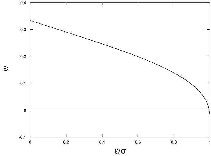
Figure 1: $w$-$\epsilon/\sigma$ diagram of the BI matter.

Before studying the evolution of the universe, we point out an interesting feature. As $\epsilon/\sigma\ll 1$ we can expand $\rho$ and $P$ as

$$\rho=\sum_{n=1}^{\infty}{}^{(n)}\!\rho,$$ (31)

$$P=\sum_{n=1}^{\infty}{}^{(n)}\!P,$$ (32)

where ${}^{(n)}\!\rho=O(\epsilon^{n})$ and ${}^{(n)}\!P=O(\epsilon^{n})$. Then we can see

$${}^{(n)}P=\frac{1}{3}{}^{(n)}\rho,~{}~{}{\rm for}~{}~{}n={\rm odd},$$ (33)

and

$${}^{(n)}\rho=-{}^{(n)}P,~{}~{}{\rm for}~{}~{}n={\rm even}.$$ (34)

The $n=$odd and $n=$even order parts behave like radiation and vacuum energy, respectively.

III.2 Evolution of universe

By using the energy conservation law, $\dot{\rho}_{\rm BI}+3H(\rho_{\rm BI}+P_{\rm BI})=0$, on the brane, the scale factor dependence of the energy density is fixed as $\rho\sim a^{-3(1+w)}$. At the low and high energy regimes, $\rho_{\rm BI}\propto a^{-4}$ and $\propto a^{-2\pi/(\pi-1)}$, respectively.

To see the qualitative evolution of the universe, the following rearrangement of the generalized Friedmann equation is useful,

$$a^{\prime 2}+V(a)=-\bar{K},$$ (35)

where

$$V(a)=-a^{2}\bar{\rho}_{\rm BI}(2+\bar{\rho}_{\rm BI}),$$ (36)

and we have normalized the variables as $\bar{t}:=t/\ell$, $\bar{\rho}_{\rm BI}:=\rho_{\rm BI}/\sigma$, $\bar{P}_{\rm BI}:=P_{\rm BI}/\sigma$, $\bar{\epsilon}:=\epsilon/\sigma$, $\bar{K}:=K\ell^{2}$. A prime denotes differentiation with respect to $\bar{t}$.

From the energy conservation law, we find

$$\bar{\epsilon}^{\prime}=\frac{4a^{\prime}}{a}{\rm arcsin}(\bar{\epsilon})\left[\frac{1}{\bar{\epsilon}^{2}}{\rm arcsin}(\bar{\epsilon})-\left(\frac{1}{\bar{\epsilon}}+1\right)\frac{1}{\sqrt{1-\bar{\epsilon}^{2}}}\right]^{-1}.$$ (37)

Solving the Eqs. (35) and (37) simultaneously, we obtain the evolution of the universe. Fig. 2 is the $a$-$\bar{\epsilon}$ diagram. For the truncated system $\bar{\epsilon}$ behaves as $\propto a^{-4}$ in the late time while it gradually increases beyond $\bar{\epsilon}=1$ as the scale factor becomes small. This regime is beyond the application of the analysis of the perturbation. On the other hand, the solution of full order is terminated when $\bar{\epsilon}=1$. Around $\bar{\epsilon}=1$, the Eq. (37) is approximated as

$$\bar{\epsilon}^{\prime}\simeq-\frac{\pi a^{\prime}}{a}\sqrt{1-\bar{\epsilon}^{2}}.$$ (38)

Then we find the solution

$$\bar{\epsilon}=\cos\left[\pi\ln\left(\frac{a}{a_{0}}\right)\right].$$ (39)

Hence for the finite value $a=a_{0}$, $\bar{\epsilon}$ becomes the critical value $\bar{\epsilon}=1$. It is interesting that the physical variables such as $\rho_{\rm BI}$, $P_{\rm BI}$, $\epsilon$ and curvatures do not diverge at this point.

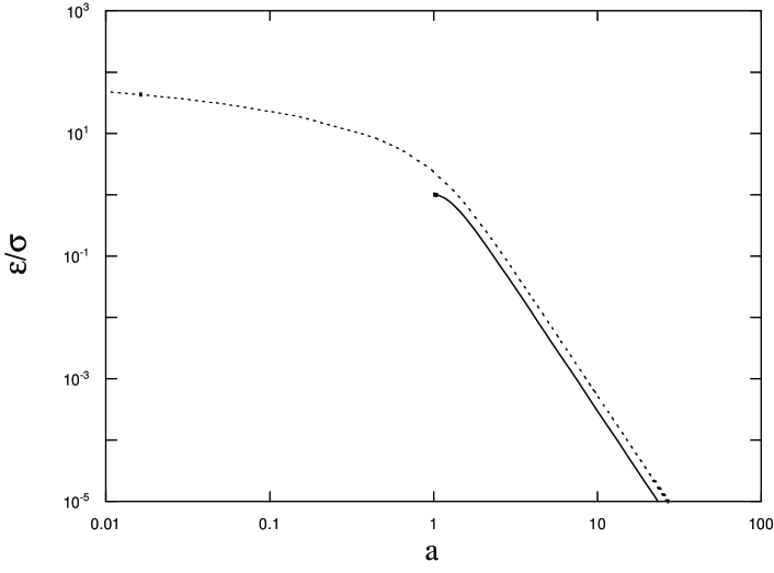
Figure 2: The $a$-$\bar{\epsilon}$ diagram of the full order (solid line) and the truncated (dashed line) systems.

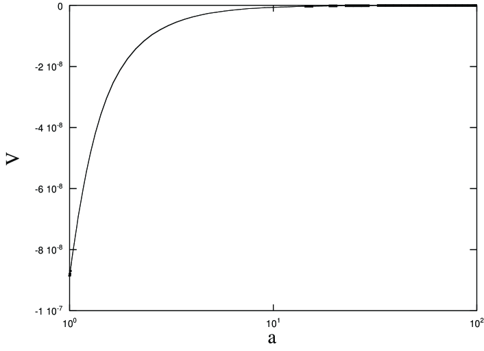
Figure 3: The configuration of the potential function of the generalized Friedmann equation.

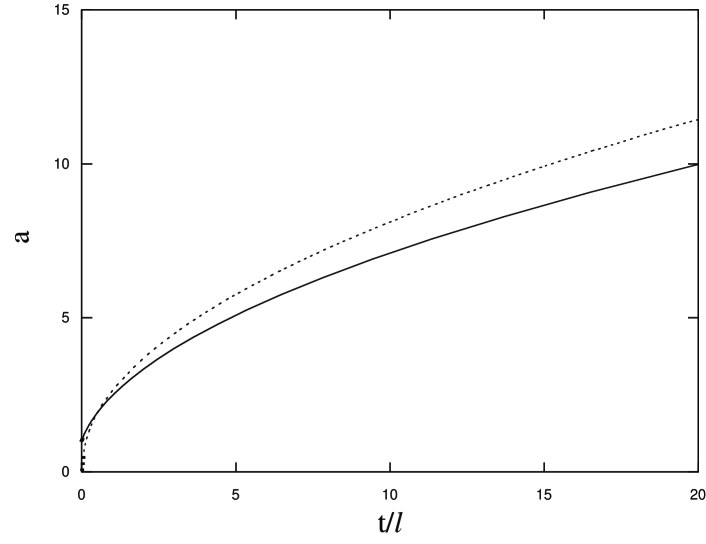
Figure 4: The evolution of the scale factor in the $K=0$ case of the full order (solid line) and the truncated (dashed line) systems.

The configuration of the potential is shown in Fig. 3. In the limit of $\bar{\epsilon}\to 1$ the potential function does not diverge unlike the ordinary radiation or matter field nor vanish unlike the truncated system in the previous work but converges non-zero finite value. We show the evolution of the scale factor in the case of $K=0$ in Fig. 4. While in the truncated system the scale factor diverges with the initial singularity, it starts from finite value at $t=t_{0}$ in the full order case.

Then there arises a question: what is the state of the universe before the time $t=t_{0}$. If we consider the quantum creation of the universe in this system, we can expect that the Euclidean action takes minimum value at $a_{0}$ somehow and that it becomes very large or even diverges beyond this point. As a result, the universe starts from $a=a_{0}$. Other possibility is that there is a reflection symmetry with respect to $t_{0}$. Since the scale factor is not connected smoothly, we can guess that there is a S-brane sbrane like structure at $t=t_{0}$. In this scenario, the universe experiences a bounce. However, we have to tune the tension of the S-brane.

It is sure that the evolution of the universe in the early stage is affected by taking into account the higher order corrections of the $\alpha^{\prime}$ expansion.

IV Summary

In this paper we considered the homogeneous and isotropic universe on the D-brane. The matter (gauge field) is automatically included in the BI action and there are higher order correction terms. The EOS is like radiation at the low energy scale and almost dust-like at the high energy scale. In high energy scales of braneworld, the $\rho^{2}$ term dominates and then the scale factor becomes $a(t)\propto t^{(\pi-1)/(2\pi)}$. This model is limited below $\bar{\epsilon}=1$ similar to the result in the Born and Infeld’s original paper OBI . At the critical value of $\bar{\epsilon}=1$, however, physical quantities are finite. Hence one might want to extend to the past. On a classical level, a mild singularity which is a jump of the expansion rate of the universe occurs. To resolve this mild singularity an introduction of a S-brane seems to be important.

The present result is quite different from the previous study DBC where truncated theory was employed. Since the truncation is often used in higher derivative theory for non-adequate regime, the previous trial study is still worthy as a first step. From the present study, however, we learned that such rough truncation approach does not give us good predictions.

Finally we should comment on our model. We assumed that the bulk stress tensor is composed of a negative cosmological constant and the brane action is BI one. In Ref. DBC3 , it is claimed that the gauge field cannot be a source of gravity on the D-brane without a cosmological constant. To recover the ordinary Einstein equation, the presence of a net cosmological constant is essential. We should take into account the above issues to obtain a firm picture of D-braneworld cosmology.

References

(1)
L. Randall and R. Sundrum, Phys. Rev. Lett. 83, 3370 (1999).
(2)
L. Randall and R. Sundrum, Phys. Rev. Lett. 83, 4690 (1999).
(3)
T. Shiromizu, K. Maeda and M. Sasaki, Phys. Rev. D62, 024012 (2000);
M. Sasaki, T. Shiromizu and K. Maeda, Phys. Rev. D62, 024008 (2000).
(4)
R. Maartens, Phys. Rev. D62, 084023(2000).
(5)
A. Chamblin and H. S. Reall, Nucl. Phys. B562,133(1999);
T. Nihei, Phys. Lett. B465, 81(1999);
N. Kaloper, Phys. Rev. D60, 123506(1999);
H. B. Kim and H. D. Kim, Phys. Rev. D61, 064003(2000);
P. Kraus, JHEP 9912, 011(1999);
D. Ida, JHEP 0009, 014(2000);
E. E. Flanagan, S.H.H. Tye and I. Wasserman,
Phys. Rev. D62, 044039(2000);
A. Chamblin, A. Karch, A. Nayeri, Phys. Lett. B509, 163(2001);
P. Bowcock, C. Charmousis and R. Gregory, Class. Quant. Grav. 17,4745(2000);
S. Mukohyama, Phys. Lett. B473, 241(2000);
J. Garriga and M. Sasaki, Phys. Rev. D62,043523(2000);
S. Mukohyama, T. Shiromizu and K. Maeda, Phys. Rev. D62, 024028(2000).
(6)
For the review, A. A. Tseytlin, hep-th/9908105.
(7)
T. Shiromizu, K. Koyama, S. Onda and T. Torii, Phys. Rev. D68,063506(2003).
(8)
T. Shiromizu, K. Koyama and T. Torii, hep-th/0307151,
to appear in Phys. Rev. D(2003).
(9)
S. Kachru, R. Kallosh, A. Linde, J. Maldacena, L. McAllister and S. P. Trivedi,
hep-th/0308055;
C. P. Burgess, P. Martineau, F. Quevedo and R. Rabadan, JHEP 06, 037(2003);
C. P. Burgess, N. E. Grandi, F. Quevedo and R. Rabadan, hep-th/0310010.
(10)
S. Alexander, R. Rrandenberger and D. Easson, Phys. Rev. D62,
103509(2000);
S. A. Abel, K. Freese and I. I. Kogan, JHEP 01, 039(2001);hep-th/0205317.
(11)
V. A. De Lorenci, R. Klippert, M. Novello and J. M. Salim, Phys. Rev. D65, 063501(2002)
(12)
R. Garcia-Salccdo and N. Breton, Int. J. Mod. Phys. A15, 4341(2000);
V. V. Dyadichev, D. V. Gal’tsov, A. G. Zorin and M. Yu. Zoyov, Phys. Rev.
D65, 084007(2002);
R. Garcia-Salccdo and N. Breton, hep-th/0212130.
(13)
T. Shiromizu, T. Torii and T. Ueusgi, Phys. Rev. D67, 123517(2003).
(14)
M. Sami, N. Dadhich and T. Shiromizu, Phys. Lett. B568, 118(2003).
(15)
M. Gutperle and A. Strominger, JHEP 0204, 018(2002).
(16)
M. Born and L. Infeld, Proc. Royal Soc. London A144, 425(1934).