A reality proof in ${\mathcal{}P}{\mathcal{}T}$-symmetric quantum mechanics

Abstract

We review the proof of a conjecture concerning the reality of the spectra of certain ${\mathcal{}P}{\mathcal{}T}$-symmetric quantum mechanical systems, obtained via a connection between the theories of ordinary differential equations and integrable models. Spectral equivalences inspired by the correspondence are also discussed.

1 Introduction

The unexpected reality of the spectra of a class of non-Hermitian quantum mechanical systems has provoked a fair amount of work since the first example was noted by Bessis and Zinn-Justin [1]. Generalising the result at $M=3/2$, a numerical study of the Schrödinger equations

$$-\frac{d^{2}}{dx^{2}}\psi(x)-(ix)^{2M}\psi(x)=E\psi(x)$$ (1)

led Bender and Boettcher to conjecture that under suitable boundary conditions the spectrum of (1) was entirely real and positive provided $M\geq 1$ [2].

Bender and Boettcher also noticed the relevance of ${\mathcal{}P}{\mathcal{}T}$-symmetry [2, 3] to these problems. For all $M$, the potentials $V(x)=-(ix)^{2M}$ are invariant under the combined action of parity and time reversal, and this implies the eigenvalues are either real or occur in complex-conjugate pairs. If all energy eigenstates are also eigenstates of the ${\mathcal{}P}{\mathcal{}T}$ operator, then the spectrum is guaranteed to be entirely real, but this is not true in general: the ${\mathcal{}P}{\mathcal{}T}$-symmetry can be spontaneously broken, in which case the corresponding energies occur in complex-conjugate pairs. In fact, a proof of the reality conjecture has only recently been obtained [4], via a correspondence between ordinary differential equations and integrable models (the so-called ‘ODE/IM correspondence’ [5, 6, 7, 8]). Here we review the proof and touch on a few of the byproducts of the correspondence relevant to the ODE community.

Generalising the Bessis – Zinn-Justin and Bender – Boettcher Hamiltonians, we consider the class of ${\mathcal{}P}{\mathcal{}T}$-symmetric problems

$$\left[-\frac{d^{2}}{dx^{2}}-(ix)^{2M}-\alpha(ix)^{M-1}+\frac{l(l+1)}{x^{2}}\right]\psi(x)=\lambda\psi(x)\quad,\quad\psi(x)\in L^{2}({\mathcal{}C})~{}.$$ (2)

For $M<2$, the contour ${\mathcal{}C}$ may be taken to be the real axis with a small dip below the origin if $l(l+1)\neq 0$. For larger $M$, the contour should be distorted into the complex plane to ensure the correct analytical continuation of the original problem, as explained in [2]. The result of [4] is that the spectrum of (2) is real for $M\geq 1$ and $\alpha<M+1+|2l+1|$ and positive for $M\geq 1$ and $\alpha<M+1-|2l+1|$ . Referring to figure 1, reality was proven for $(\alpha,l)\in B\cup C\cup D$, and positivity for $(\alpha,l)\in D$.

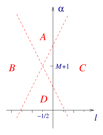
Fig. 1. : The initial ‘phase diagram’ at fixed $M$.

2 The functional relation

Rather than considering the ${\mathcal{}P}{\mathcal{}T}$-symmetric problem (2) alone, we introduce a related problem obtained from (2) by sending $x\to x/i$ and $E\to-E$:

$$\left(-\frac{d^{2}}{dx^{2}}+x^{2M}\pm\alpha x^{M-1}+\frac{l(l{+}1)}{x^{2}}\right)\Phi(x)=E\Phi(x)~{}.$$ (3)

It will be convenient to treat positive and negative values of $\alpha$ together. The boundary conditions for (3) are that $\Phi(x)$ should vanish as $x\to\infty$ along the real axis, and behave as $x^{l+1}$ as $x\to 0$. For $l$ real and larger than $-1/2$, this problem is Hermitian. In the language of ordinary differential equations in the complex domain, it is sometimes called a ‘radial’ problem, while (2) is called a ‘lateral’ problem. (Note, the radial problem can also be considered for $\Re e\,l\leq-1/2$, but is best then defined by analytic continuation in $l$.)

Following the ideas particularly advocated by Sibuya and Voros in the context of ordinary differential equations [9, 10], we approach the spectral problems by studying the behaviour of the associated spectral determinants. Adopting the convention used in [15], let $\{E_{j}^{(\pm)}\}$ be the set of eigenvalues of (2) with inhomogeneous term $\mp\alpha(ix)^{M{-}1}$, and let $\{e_{i}^{(\pm)}\}$ be the eigenvalues of (3) with inhomogeneous term $\pm\alpha x^{M{-}1}$. Then define two pairs of spectral determinants, as follows:

$$T^{(\pm)}(E)=T^{(\pm)}(0)\prod_{j=0}^{\infty}\left(1+\frac{E}{E^{(\pm)}_{j}}\right)~{},$$ (4)

and

$$Q^{(\pm)}(E)=Q^{(\pm)}(0)\prod_{i=0}^{\infty}\left(1-\frac{E}{e^{(\pm)}_{i}}\right)~{}.$$ (5)

Both products are convergent for $M>1$, and define entire functions of $E$, and their zeroes (or, for $T(E)$, their negatives) coincide with the eigenvalues of the corresponding spectral problem. For $M\leq 1$ convergence factors must be added, and it is more efficient to define the spectral determinants indirectly, via certain special ‘Sibuya’ solutions to (3), which are anyway needed to prove the key identity (6) below; see [9, 7] for more details.

By considering the asymptotic behaviour of the Sibuya solutions in the complex plane it is not hard, following the arguments given in [7], to establish a Stokes relation, from which one can obtain the following functional equations

$$T^{(\pm)}(E)Q^{(\pm)}(E)=\omega^{-(2l+1\pm\alpha)/2}Q^{(\mp)}(\omega^{-2}E)+\omega^{(2l+1\pm\alpha)/2}Q^{(\mp)}(\omega^{2}E)~{},$$ (6)

where $\omega=e^{i\pi/(M+1)}$. This shows that the spectral problems (2) and (3) are related by much more than a simple change of variables and boundary conditions, and also that the spectral problem at positive $\alpha$ is necessarily tied up with the problem at negative $\alpha$. Furthermore, this functional relation taken at $\alpha=0$ is well-known in the integrable model (IM) world, where it goes by the name of Baxter’s TQ relation. This observation, initially developed in [5, 6, 7], has led to an exact mapping between ODE quantities such as spectral determinants and functions constructed in the context of integrable models. It provides a powerful tool to analyse ODE problems using IM techniques, and vice-versa.

If we set $E=e^{(\mp)}_{j}$ in (6) we can use the entirety of $T$ and the product form for $Q$ (5) to obtain

$$\prod_{i=0}^{\infty}\left(\frac{e_{i}^{(\mp)}-\omega^{2}e^{(\pm)}_{j}}{e^{(\mp)}_{i}-\omega^{-2}e^{(\pm)}_{j}}\right)=-\omega^{-2l-1\mp\alpha}\,.$$ (7)

In IM language sets of coupled equations of this type are known as Bethe ansatz equations. Their solution allows $Q$ to be reconstructed via (5) and thus $T$ using the TQ relation (6). Finally the eigenvalues of the ${\mathcal{}P}{\mathcal{}T}$-symmetric Hamiltonian are found by searching for the zeros of $T(E)$. Alternatively, a technique developed in integrable models allows one to convert the Bethe ansatz equations (7) into a single nonlinear integral equation, from which one can easily numerically obtain both the zeros of $Q(E)$ and $T(E)$, as first emphasised in [5, 7].

3 The proof

Returning to the reality proof, a second set of Bethe ansatz like equations can be obtained from (6) if we instead set $E=-E^{(+)}_{j}$ and invoke the entirety of $Q^{(-)}(E)$. Rearranging and using the product form (5) leads to

$$\prod_{i=0}^{\infty}\left(\frac{e^{(-)}_{i}+\omega^{2}E^{(+)}_{j}}{e^{(-)}_{i}+\omega^{-2}E^{(+)}_{j}}\right)=-\omega^{-2l-1-\alpha}\,.$$ (8)

This equation couples the so-far mysterious eigenvalue $E^{(+)}_{j}$ of the ${\mathcal{}P}{\mathcal{}T}$-symmetric problem (2) to the much better-controlled eigenvalues of the Hermitian problem (3). Indeed, a Langer transformation [11] shows that the eigenvalues $e^{(-)}$ of the radial problem are also positive if $\alpha<M+2l+2$ [4]. It is from this equation that we are able to prove the reality of the ${\mathcal{}P}{\mathcal{}T}$-symmetric problem.

The first step will be to set $E^{(+)}_{j}=|E^{(+)}_{j}|\exp(i\,\delta_{k})$. Now take the modulus² of (8) to obtain

$$\prod_{i=0}^{\infty}\left(\frac{(e^{(-)}_{i})^{2}+|E^{(+)}_{j}|^{2}+2\,e^{(-)}_{i}\,|E^{(+)}_{j}|\cos({\textstyle\frac{2\pi}{M+1}}+\delta_{j})}{(e^{(-)}_{i})^{2}+|E^{(+)}_{j}|^{2}+2\,e^{(-)}_{i}\,|E^{(+)}_{j}|\cos({\textstyle\frac{2\pi}{M+1}}-\delta_{j})}\right)=1\,.$$ (9)

For $\alpha<M+2l+2$ all the $e^{(-)}_{i}$ are positive, and each single term in the product on the LHS of (9) is either greater than, smaller than, or equal to one depending only on the relative values of the cosine terms in the numerator and denominator. These are independent of the index $i$. Therefore the only possibility to match the RHS is for each term in the product to be individually equal to one, which for $E^{(+)}_{j}\neq 0$ requires

$$\cos({\textstyle\frac{2\pi}{M+1}}+\delta_{j})=\cos({\textstyle\frac{2\pi}{M+1}}-\delta_{j})~{},\quad\mbox{or}\quad\sin({\textstyle\frac{2\pi}{M{+}1}})\sin(\delta_{j})=0\,.$$ (10)

Since $M>1$, this latter condition implies

$$\delta_{j}=n\pi\,,~{}~{}~{}~{}n\in{\mathbb{Z}}$$ (11)

and this establishes the reality of the eigenvalues of (2) for $M>1$ and $\alpha<M+2l+2$ or, relaxing the condition on $l$, $\alpha<M+1+|2l{+}1|$.

At $M\leq 1$ the simple form (5) for $D^{(-)}(E)$ acquires extra convergence factors, resulting in a break down of the proof, as expected given the numerical findings of [2, 7]. More details can be found in [4]; for a further generalisation of the method, see [12].

Finally, we remark that while the above constraints on the parameters $M,\alpha$ and $l$ are sufficient conditions they are not necessary, as demonstrated in figure 2 for the case $M=3$. The full domain of unreality, obtained numerically in [13], is the interior of the curved line, a proper subset of $A$ which only touches its boundary at isolated points. In the small, approximately-triangular region inside $A$ but outside the curved line which abuts the crossing of the lines separating the regions $A,B,C,D$, the spectrum is not only real but also entirely positive, despite the fact that it lies outside the domain $D$. The separating lines themselves have further significance, in that at these points the model has a hidden supersymmetry, which plays a significant rôle in the breakdown of reality [13].

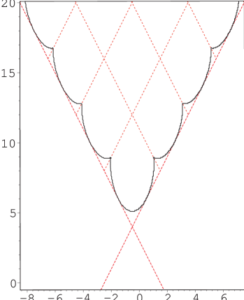
Fig. 2. : The domain of unreality for $M=3$. Horizontal and vertical axes are $l$ and $\alpha$ respectively.

4 Further consequences

One further application of the ODE/IM correspondence was also found in [4], and concerns the lateral and radial problems at $M=3$. As remarked in [21], it is convenient to reparametrise the angular-momentum term by setting $\lambda=\sqrt{3}(2l{+}1)$ , so that the equation becomes

$$\left(-\frac{d^{2}}{dx^{2}}+x^{6}+\alpha x^{2}+\frac{\lambda^{2}-3}{12\,x^{2}}\right)\Phi(x)=E\Phi(x)~{}.$$ (12)

Define $\boldsymbol{\alpha}=(\alpha,\lambda)^{T}$ and let $D(E,\boldsymbol{\alpha})$ denote the spectral determinant for this problem. Via the Bethe ansatz approach, it turns out that this problem has a relationship with a third-order ordinary differential equation:

$$\left({\mathrm{D}}(g_{2}{-}2){\mathrm{D}}(g_{1}{-}1){\mathrm{D}}(g_{0})+x^{3}\right)\phi=\frac{3\sqrt{3}}{4}\,E\phi$$ (13)

where ${\mathrm{D}}(g)\equiv(\frac{d}{dx}-\frac{g}{x})$, and

$$g_{0}=1+(\alpha+\sqrt{3}\lambda)/4~{}~{},~{}~{}g_{1}=1+\alpha/2~{}~{},~{}~{}g_{2}=1+(\alpha-\sqrt{3}\lambda)/4~{}.$$ (14)

This third-order equation is associated with $SU(3)$ Bethe ansatz equations, as discussed in [14, 15]. Furthermore, the third-order equation is symmetrical in $\{g_{0},g_{1},g_{2}\}$, a feature which is completely hidden in the original second-order equation. By playing with this symmetry, one can establish some novel spectral equivalences between different (second-order) radial problems, and also between these and certain lateral problems. We add to the results discussed in [4] the remark that, when expressed in terms of the parameters $(\alpha,\lambda)$, the mappings turn out to act as certain $2\times 2$ matrices in the Weyl group of $SU(3)$. The matrices ${\mathbb{L}}$ and ${\mathbb{T}}$ defined as

$${\mathbb{L}}=\left(\begin{array}[]{cc}1&0\\ 0&-1\end{array}\right)\quad\,,\quad{\mathbb{T}}=\frac{1}{2}\left(\begin{array}[]{cc}-1&\sqrt{3}\\ -\sqrt{3}&-1\end{array}\right)$$ (15)

generate the Weyl group of $SU(3)$, the matrix ${\mathbb{L}}$ describing a rotation and ${\mathbb{T}}$ a reflection. In [4] we found a spectral equivalence between a pair of radial problems

$$\gamma(\boldsymbol{\alpha})D(E,\boldsymbol{\alpha})=\gamma({\mathbb{T}}\boldsymbol{\alpha})D(E,{\mathbb{T}}\boldsymbol{\alpha})~{},$$ (16)

where $\gamma(\boldsymbol{\alpha})=2\sqrt{i\pi}/\Gamma(\lambda/2\sqrt{3})$. An equivalence was also obtained at a particular set of points for which the radial problem $D(E,\boldsymbol{\alpha})$ has a quasi-exactly solvable sector [16, 17]. For positive integer $J$ and $\boldsymbol{\alpha}_{J}=-(4J+\lambda/\sqrt{3},\lambda)$, the first $J$ levels of $D(E,\boldsymbol{\alpha}_{J})$ can be computed exactly as the zeros of the Bender-Dunne polynomials $P_{J}(E)$ [18]. The result is that modulo the QES levels, the problems $D(E,{\mathbb{T}}{\mathbb{L}}\boldsymbol{\alpha}_{J})$ and $D(E,\boldsymbol{\alpha}_{J})$ are isospectral.

A further spectral equivalence particularly relevant to the main theme of this paper occurs between a radial problem and the related lateral problem (2) taken at $M=3$. The equivalence is

$$T(-E,\boldsymbol{\alpha})=\gamma({\mathbb{L}}{\mathbb{T}}\boldsymbol{\alpha})D(E,{\mathbb{L}}{\mathbb{T}}\boldsymbol{\alpha})~{}.$$ (17)

If we denote ${\mathbb{L}}{\mathbb{T}}\boldsymbol{\alpha}=(\tilde{\alpha},\tilde{\lambda})^{T}$ then the problem on the RHS is Hermitian for $\tilde{\lambda}>0$, and this relation provides a simple explanation for the reality of the spectrum of the ${\mathcal{}P}{\mathcal{}T}$-symmetric problems in these particular cases. At the points $\boldsymbol{\alpha}=\boldsymbol{\alpha}_{J}$ we can combine the dualities to prove a simple result concerning the spectrum of $T(E,\boldsymbol{\alpha}_{J})$, namely that the only energies to become complex as the parameters $(\alpha,l)$ move into region $A$ through QES values lie in the solvable part of the spectrum [13]. This adds to a similar, as yet unproven, conjecture concerning quartic QES potentials [22].

More detailed reviews of the ODE/IM correspondence, with more extensive sets of references, can be found in [19, 20, 21]. The original correspondence relates only the groundstate of a quantum field theory to an ODE, but recently a set of differential equations has been found for the excited states of the field theory [23]. Further aspects of the correspondence are still being developed, and much remains to be understood. In particular, it would be valuable to have a more physical insight into why the relationship between integrable quantum field theories and ordinary differential equations should be so close. As more examples are uncovered, we can start to hope that progress on this so-far mysterious issue may not be too far away.

Acknowledegments –  TCD thanks the organisers for the opportunity to speak at the conference; TCD and RT thank the UK EPSRC for a Research Fellowship and an Advanced Fellowship respectively. This work was partially supported by the EC network “EUCLID”, contract number HPRN-CT-2002-00325.

References

- [1] D. Bessis and J. Zinn-Justin: unpublished, circa 1992.
- [2] C.M. Bender and S. Boettcher: Phys. Rev. Lett. 80 (1998) 4243.
- [3] C.M. Bender, S. Boettcher and P.N. Meissinger: J. Math. Phys. 40 (1999) 2201.
- [4] P. Dorey, C. Dunning and R. Tateo: J. Phys. A: Math. Gen. 34 (2001) 5679.
- [5] P. Dorey and R. Tateo: J. Phys. A32 (1999) L419.
- [6] V.V. Bazhanov, S.L. Lukyanov and A.B. Zamolodchikov: J. Stat. Phys. 102 (2001) 567.
- [7] P. Dorey and R. Tateo: Nucl. Phys. B563 (1999) 573.
- [8] J. Suzuki: J. Stat. Phys. 102 (2001) 1029.
- [9] Y. Sibuya, Global Theory of a second-order linear ordinary differential equation with a polynomial coefficient. Amsterdam: North-Holland, 1975.
- [10] A. Voros: J. Physique Lett. 43 (1982) L1; Ann. Inst. Henri Poincaré XXXIX (1983) 211; J. Phys. A: Math. Gen. 32 (1999) 5999; Corrigendum J. Phys. A: Math. Gen. 34 (2000) 5783.
- [11] R.E. Langer: Phys. Rev. 51 (1937) 669.
- [12] K. C. Shin: Commun. Math. Phys. 229 (2002) 543.
- [13] P. Dorey, C. Dunning and R. Tateo: J. Phys. A: Math. Gen. 34 (2001) L391.
- [14] P. Dorey and R. Tateo: Nucl. Phys. B571 (2000) 583.
- [15] P. Dorey, C. Dunning and R. Tateo: J. Phys. A: Math. Gen. 33 (2000) 8427.
- [16] A.V. Turbiner: Comm. Math. Phys. 118 (1988) 467.
- [17] A.G. Ushveridze: Quasi-Exactly Solvable Models in Quantum Mechanics. Institute of Physics, Bristol, 1993.
- [18] C.M. Bender and G.V. Dunne: J. Math. Phys. 37 (1996) 6.
- [19] P. Dorey, C. Dunning and R. Tateo: in Proceedings of Nonperturbative Quantum Effects, Paris, 2000 JHEP Proceedings PRHEP-tmr 2000/034, hep-th/0010148.
- [20] P. Dorey, C. Dunning and R. Tateo: in Proceedings of the Johns Hopkins workshop on current problems in particle theory 24, Budapest, 2000. World Scientific, 2001.
- [21] P. Dorey, C. Dunning, A. Millican-Slater and R. Tateo: in Proceedings of the 14th International Congress on Mathematical Physics, Lisbon 2003. World Scientific. hep-th/0309054.
- [22] C.M. Bender and S. Boettcher: J. Phys. A31 (1998) L273.
- [23] V.V. Bazhanov, S.L. Lukyanov and A.B. Zamolodchikov: Higher-level eigenvalues of Q-operators and Schrödinger equation, hep-th/0307108.