hep-th/0309208
HUTP-03/A061

Quantum Calabi-Yau and Classical Crystals

Andrei Okounkov¹, Nikolai Reshetikhin², and Cumrun Vafa³

¹Department of Mathematics,
Princeton University, Princeton, NJ 08544, U.S.A.
okounkov@math.princeton.edu

²Department of Mathematics,
University of California at Berkeley, Evans Hall, # 3840, Berkeley, CA 94720-3840, U.S.A.
reshetik@math.berkeley.edu

³Jefferson Physical Laboratory, Harvard University,
Cambridge, MA 02138, U.S.A.
vafa@string.harvard.edu

We propose a new duality involving topological strings in the limit of large string coupling constant. The dual is described in terms of a classical statistical mechanical model of crystal melting, where the temperature is inverse of the string coupling constant. The crystal is a discretization of the toric base of the Calabi-Yau with lattice length $g_{s}$. As a strong evidence for this duality we recover the topological vertex in terms of the statistical mechanical probability distribution for crystal melting. We also propose a more general duality involving the dimer problem on periodic lattices and topological A-model string on arbitrary local toric threefolds. The $(p,q)$ 5-brane web, dual to Calabi-Yau, gets identified with the transition regions of rigid dimer configurations.

1 Introduction

Topological strings on Calabi-Yau threefolds have been a fascinating class of string theories, which have led to insights into dynamics of superstrings and supersymmetric gauge theories. They have also been shown to be equivalent in some cases to non-critical bosonic strings. In this paper we ask how the topological A-model which ‘counts’ holomorphic curves inside the Calabi-Yau behaves in the limit of large values of the string coupling constant $g_{s}\gg 1$. We propose a dual description which is given in terms of a discrete statistical mechanical model of a three dimensional real crystal with boundaries, where the crystal is located in the toric base of the Calabi-Yau threefold, with the ‘atoms’ separated by a distance of $g_{s}$. Moreover the Temperature $T$ in the statistical mechanical model corresponds to $1/g_{s}$. Heating up the crystal leads to melting of it. In the limit of large temperature, or small $g_{s}$, the Calabi-Yau geometry emerges from the geometry of the molten crystal !

In the first part of this paper we focus on the simplest Calabi-Yau, namely ${\bf C}^{3}$. Even here there are a lot of non-trivial questions to answer. In particular the computation of topological string amplitudes when we put D-branes in this background is non-trivial and leads to the notion of a topological vertex [1, 2] (see also the recent paper [3]). Moreover using the topological vertex one can compute an all order amplitude for topological strings on arbitrary local Calabi-Yau manifolds. This is an interesting class to study, as it leads to non-trivial predictions for instanton corrections to gauge and gravitational couplings of a large class of $N=2$ supersymmetric gauge theories in 4 dimensions via geometric engineering [4] (for recent progress in this direction see [5, 6]). It is also the same class which is equivalent (in some limits) to non-critical bosonic string theories. In this paper we will connect the topological vertex to the partition function of a melting corner with fixed asymptotic boundary conditions. Furthermore we find an intriguing link between dimer statistical mechanical models and non-compact toric Calabi-Yau threefolds. In particular the dimer problems in 2 dimensions naturally get related to the study of configurations of $(p,q)$ 5-brane web, which is dual to non-compact toric Calabi-Yau threefolds.

The organization of this paper is as follows: In Section 2 we will motivate and state the conjecture. In Section 3 we check aspects of this conjecture and derive the topological vertex from the statistical mechanical model. In Section 4 we discuss dimer problems and its relation to topological strings on Calabi-Yau.

Our proposal immediately raises many questions, which are being presently investigated. Many of them will be pointed out in the paper. One of the most interesting physical questions involves the superstring intepretation of the discretization of space. On the mathematical side, we expect that our statistical mechanical model should have a deep meaning in terms of the geometry of target space based on the interpretation of its configurations as torus fixed points in the Hilbert scheme of curves of the target threefold. Also, our 3d model naturally extends the random 2d partition models that arise in $N=2$ supersymmetric gauge theory [5] and Gromov-Witten theory of target curves [7]. For some mathematical aspects of the topological vertex see [8, 9, 3].

2 The Conjecture

2.1 Hodge integrals and 3d partitions

Consider topological A-model strings on a Calabi-Yau threefold. For simplicity, let us consider the limit when the Kähler class of Calabi-Yau is rescaled by a factor that goes to infinity. As explained in [10] in this limit the genus $g$ amplitude is given by

$$\frac{\chi}{2}\int_{\overline{\mathcal{M}}_{g}}c_{g-1}^{3}({\mathcal{H}})$$

where $\chi$ is the Euler characteristic of the Calabi-Yau threefold, $\overline{\mathcal{M}}_{g}$ is the moduli space of Riemann surfaces, ${\cal H}$ is the Hodge bundle over $\overline{\mathcal{M}}_{g}$, and $c_{g-1}$ denotes the $(g-1)$-st Chern class of it. For genus 0 and 1, there are also some Kähler dependence (involving volume and the second Chern class of the tangent bundle), which we subtract out to get a finite answer. Consider

$$Z=\exp\left[\frac{\chi}{2}\sum_{g}g_{s}^{2g-2}\int_{\overline{\mathcal{M}}_{g}}c_{g-1}^{3}({\cal H})\right]\,.$$

It has been argued physically [11] and derived mathematically [12] that

$$Z=f^{\chi/2}$$

where

$$f=\prod_{n}{1\over(1-q^{n})^{n}}$$

and

$$q=e^{-g_{s}}\,.$$

By the classical result of McMahon, the function $f$ is the generating function for 3d partitions, that is,

$$f=\sum_{\textup{3d partitions}}q^{\textup{\# boxes}}\,,$$

where, by definition, a 3d partition is a 3d generalization of 2d Young diagrams and is an object of kind seen on the left in Figure 3. This fact was pointed out to one of us as a curiosity by R. Dijkgraaf shortly after [11] appeared.

2.2 Melting of a crystal and Calabi-Yau threefold

It is natural to ask whether there is a deeper reason for this correspondence. What could three dimensional partitions have to do with A-model topological string on a Calabi-Yau threefold ? The hint comes from the fact that we are considering the limit of large Kähler class and in this limit the Calabi-Yau looks locally made of $\mathbf{C}^{3}$’s glued together. It is then natural to view this torically, as we often do in topological string, in the context of mirror symmetry, and write the Kähler form as

$$\sum_{i=1,2,3}dz_{i}\wedge d{\overline{z}}_{i}\sim\sum_{i=1,2,3}d|z_{i}|^{2}\wedge d\theta_{i}$$

and $|z_{i}|^{2}$ span the base of a toric fibration of $\mathbf{C}^{3}$. Note that $|z_{i}|^{2}=x_{i}$ parameterize the positive octant $O^{+}\subset\mathbf{R}^{3}$. If we assign Euler characteristic “2” to each $\mathbf{C}^{3}$ patch, the topological string amplitudes on it get related to the McMahon function. Then it is natural to think that the octant is related to the three dimensional partitions, in which the boxes are located at $\mathbf{Z}^{3}$ lattice points inside $O^{+}$. Somehow the points of the Calabi-Yau, in this case $\mathbf{C}^{3}$, become related to integral lattice points on the toric base.

The picture we propose is the following. We identify the highly quantum Calabi-Yau with the frozen crystal, that is, the crystal in which all atoms (indexed by lattice points in $O^{+}$) are in place. We view the excitations as removing lattice points as in Figure 1. The rule is that we can remove lattice points only if there are no pairs of atoms on opposite sides. This gives the same rule as 3d partitions. Note that if one holds the page upside-down, one sees a 3d partition in Figure 1, namely the partition from Figure 3.

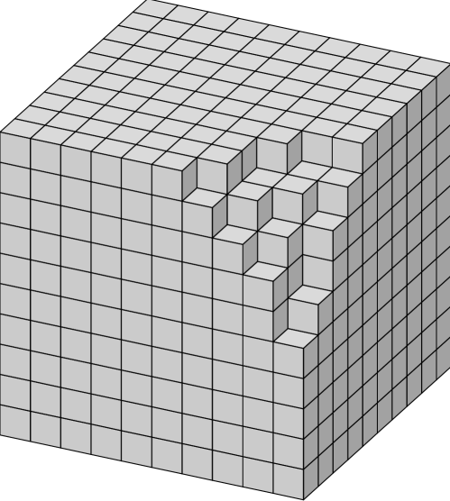
Figure 1: A melting crystal corner

Removing each atom contributes the factor $q=e^{-\mu/T}$ to the Boltzmann weight of the configuration, where $\mu$ is the chemical potential (the energy of the removal of an atom) and $T$ is the temperature. We choose units in which $\mu=1$. To connect this model to topological string on $\mathbf{C}^{3}$ we identify $g_{s}=1/T$. In particular, the $g_{s}\to 0$, that is, the $q\to 1$ limit the crystal begins to melt away. Rescaled in all direction by a factor of $1/T=g_{s}$, the crystal approaches a smooth limit shape which has been studied from various viewpoints [15, 16]. It is plotted in Figure 2.

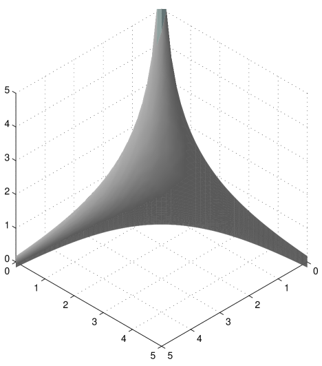
Figure 2: The limit shape of a 3d partition

The analytic form of this limit shape is encoded in terms of a complex Riemann surface, which in this case is given by

$$F(u,v)=e^{-u}+e^{-v}+1=0$$ (2.1)

defined as a hypersurface in $\mathbf{C}^{2}$ with a natural 2-form $du\wedge dv$, where $u,v$ are periodic variables with period $2\pi i$. In coordinates $e^{-u}$ and $e^{-v}$ this is simply a straight line in $\mathbf{C}^{2}$. Consider the following function of the variables $U=Re(u)$ and $V=Re(v)$

$$R(U,V)=\frac{1}{4\pi^{2}}\iint_{0}^{2\pi}\log\,|F(U+i\theta,V+i\phi)|\,d\theta d\phi\,.$$ (2.2)

This function is known as the Ronkin function of $F$. In terms of the Ronkin function, the limit shape can be parameterized as follows:

$$(x_{1},x_{2},x_{3})=(U+R,V+R,R)\,,\quad R=R(U,V)\,.$$

Note that

$$U=x_{1}-x_{3}\,,\quad V=x_{2}-x_{3}\,.$$

The projection of the curved part of the limit shape onto the $(U,V)$-plane is the region bounded by the curves

$$\pm e^{-U}\pm e^{-V}+1=0\,,$$

excluding the case when both signs are positive. This region is the amoeba of the curve (2.1), which, by definition, is its image under the map $(u,v)\mapsto(U,V)$. In different coordinates, this is the planar region actually seen in Figure 2.

2.3 Mirror symmetry and the limit shape

Consider topological strings on ${\bf C}^{3}$. One can apply mirror symmetry in this context by dualizing the three phases of the complex parameters according to T-duality. This has been done in [13]. One introduces dual variables $Y_{i}$ which are periodic, with period $2\pi i$ and are related to the $z_{i}$ by

$$|z_{i}|^{2}=ReY_{i}$$

(this is quantum mechanically modified by addition of an $i$-independent large positive constant to the right hand side). The imaginary part of the $Y_{i}$ is ‘invisible’ to the original geometry, just as is the phase of the $z_{i}$ to the $Y_{i}$ variables. They are T-dual circles. But we can compare the data between ${\bf C}^{3}$ and the mirror on the base of the toric variety which is visible to both. In mirror symmetry the Kähler form of ${\bf C}^{3}$ gets mapped to the holomorphic three form which in this case is given by

$$\Omega=\prod_{i=1}^{3}dY_{i}\ {\rm exp}[W]$$

where

$$W=\sum e^{-Y_{i}}.$$

Note that shifting $Y_{i}\rightarrow Y_{i}+r$ shifts $W\rightarrow e^{-r}W$. The analog of rescaling in the mirror is changing the scale of $W$. Let us fix the scale by requiring $W=1$; this will turn out to be the mirror statement to rescaling by $g_{s}$ to get a limit shape. In fact we will see below that the limit shape corresponds to the toric projection of the complex surface in the mirror given simply by $W(Y_{i})=1$. Let us define

$$u=Y_{1}-Y_{3},\quad v=Y_{2}-Y_{3}$$

Then

$$W=e^{-Y_{3}}F(u,v)$$

where

$$F(u,v)=e^{-u}+e^{-v}+1$$

we will identify $F(u,v)$ with the Riemann surface of of the crystal melting problem. In this context also according to mirror map the points in the $u,v$ space get mapped to the points on the toric base (i.e $O^{+}$) satisfying

$$x_{1}-x_{3}=Re(u)=U$$

$$x_{2}-x_{3}=Re(v)=V$$

We now wish to understand the interpretation of limit shape from the viewpoint of topological string. We propose that the boundary of the molten crystal which is a 2-cycle on the octant should be viewed as a special Lagrangian cycle of the A-model with one hidden circle in the fiber. Similarly in the B-model mirror it should be viewed as the B-model holomorphic surface, which in the case at hand gets identified with $W=1$ (recall that in the LG models B-branes can be identified with $W={\rm const.}$ [14]). On this surface we have

$$e^{-Y_{3}}F(u,v)=1$$

If we take the absolute value of this equation, to find the projection on to the base we find

$$e^{-Re(Y_{3})}|F(u,v)|=1$$

If we take the logarithm of this relation we have

$$-Re(Y_{3})+{\rm log}|e^{-u}+e^{-v}+1|=0\rightarrow x_{3}={\rm log}|e^{-u}+e^{-v}+1|$$

However we have a fuzziness in mapping this to the toric base: $u=Re(u)+i\theta$ and $v=Re(v)+i\phi$ and so a given value for $Re(u)$ and $Re(v)$ does not give a fixed value of $x_{3}$. That depends in addition on the angles $\theta,\phi$ of the mirror torus which are invisible to the A-model toric base. It is natural to take the average values as defining the projection to the base, i.e.

$$x_{3}={1\over 4\pi^{2}}\int d\theta d\phi\ {\rm log}|F(U+i\theta,V+i\phi)|$$

which is exactly the expression for the limit shape. We thus find some further evidence that the statistical mechanical problem of crystal melting is rather deeply related to topological string and mirror symmetry on Calabi-Yau. Moreover we can identify the points of the crystal, with the discretization of points of the base of the toric Calabi-Yau.

To test this conjecture further we will have to first broaden the dictionary between the two sides. In particular we ask what is the interpretation of the topological vertex for the statistical mechanical problem of crystal melting? For topological vertex we fix a 2d partition on each of the three legs of the toric base. There is only one natural interpretation of what this could mean in the crystal melting problem: This could be the partition function of the melting crystal with three fixed asymptotic boundary shapes for the molten crystal, dictated by the corresponding partition. We will show this is indeed the case in the next section.

3 Melting corner and the topological vertex

3.1 Transfer matrix approach

The grand canonical ensemble of 3d partitions weighted with $q^{\textup{\# boxes}}$ is the simplest model of a melting crystal near its corner. We review the transfer matrix approach to this model following [16]. This approach can be easily generalized to allow for certain inhomogeneity and periodicity, which is useful in the context of more general models discussed in Section 4.

We start by cutting the 3d partition into diagonal slices by planes $x_{2}-x_{1}=t$, see Figure 3. This operation makes a 3d partition a sequence $\{\mu(t)\}$ of ordinary partitions indexed by an integer variable $t$. Conversely, given a sequence $\{\mu(t)\}$, it can be assembled in a 3d partition provided it satisfies the following interlacing condition. We say that two partitions $\mu$ and $\nu$ interlace, and write $\mu\succ\nu$ if

$$\mu_{1}\geq\nu_{1}\geq\mu_{2}\geq\nu_{2}\geq\dots\,.$$

It is easy to see that a sequence of slices $\{\mu(t)\}$ of a 3d partition satisfies

$$\mu(t)\prec\mu(t+1)\,,\quad t<0\,,$$

and the reverse relation for $t\geq 0$.

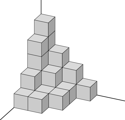
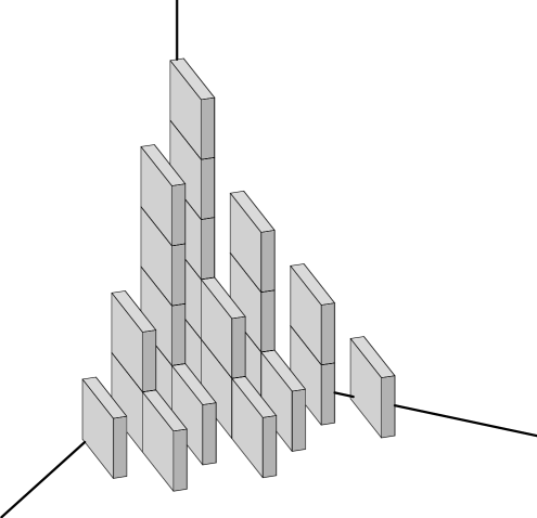
Figure 3: A 3d partition and its diagonal slices

There is a well-known map from partitions to states in the NS sector of complex fermionic oscillator. Let $a_{i}$ and $b_{i}$ be the areas of pieces one gets by slicing a 2d partition first diagonally and then horizontally (resp. vertically) above and the below the diagonal, respectively. Formally,

$$a_{i}=\mu_{i}-i+\frac{1}{2}\,,\quad b_{i}=\mu^{t}_{i}-i+\frac{1}{2}\,,$$

where $i$ ranges from 1 to the number of squares on the diagonal of $\mu$. In mathematical literature, these coordinates on partitions are known as (modified) Frobenius coordinates. The fermionic state associated to $\mu$ is

$$|\mu\rangle=\prod_{j=1}^{d}\psi^{*}_{a_{i}}\psi_{b_{i}}|0\rangle$$

Note that

$$q^{L_{0}}|\mu\rangle=q^{\textup{\# boxes}}|\mu\rangle=q^{|\mu|}|\mu\rangle\,,$$

where we denote the total number of boxes of $\mu$ by $|\mu|$. We can write a bosonic representation of this state by the standard bosonization procedure.

Consider the operators

$$\Gamma_{\pm}(z)=\exp\left(\sum_{\pm n>0}{z^{n}J_{n}\over n}\right)\,,$$

where $J_{n}$ denotes the modes of the fermionic current $\psi^{*}\psi$. The operators $\Gamma_{\pm}(z)$ can be identified with annihilation and creation parts of the bosonic vertex operator $e^{\phi(z)}$. The relevance of these operators for our problem lies in the following formulas:

$$\Gamma_{-}(1)|\mu\rangle =\sum_{\nu{\succ}\mu}|\nu\rangle$$ (3.3)

$$\Gamma_{+}(1)|\mu\rangle =\sum_{\nu{\prec}\mu}|\nu\rangle$$

To illustrate their power we will now derive, as in [16], the McMahon’s generation function for 3d partitions

$$Z=\sum_{\textup{3d partitions $\pi$}}q^{\textup{\# of boxes}}\,.$$

By the identification (3.3) of the transfer matrix, we have

$$Z=\left\langle\left(\prod_{t=0}^{\infty}q^{L_{0}}\,\Gamma_{+}(1)\right)q^{L_{0}}\left(\prod_{t=-\infty}^{-1}\Gamma_{-}(1)\,q^{L_{0}}\right)\right\rangle\,.$$ (3.4)

Now we commute the operators $q^{L_{0}}$ to the outside, splitting the middle one in half. This yields

$$Z=\left\langle\prod_{n>0}\Gamma_{+}(q^{n-\frac{1}{2}})\,\prod_{n>0}\Gamma_{-}(q^{-n-\frac{1}{2}})\right\rangle\,.$$ (3.5)

Now we commute the creation operators through annihilation operators, using the commutation relation

$$\Gamma_{+}(z)\,\Gamma_{-}(z^{\prime})=(1-z/z^{\prime})^{-1}\,\Gamma_{-}(z^{\prime})\,\Gamma_{+}(z)\,.$$

The product of resulting factors gives directly the McMahon’s function

$$Z=\prod_{n>0}(1-q^{n})^{-n}=f\,.$$

Same ideas can be used to get more refined results, such as, for example, the correlation functions, see [16]. We will generalize below the above computation to the case when 3d partitions have certain asymptotic configuration in the direction of the three axes. Before doing this, we will review some relevant theory of symmetric functions.

3.2 Skew Schur functions

Skew Schur functions $s_{\lambda/\mu}(x_{1},x_{2},\dots)$ are certain symmetric polynomials in the variables $x_{i}$ indexed by a pair of partitions $\mu$ and $\lambda$ such that $\mu\subset\lambda$, see [17]. Their relevance for us lies in the well-known fact (see e.g. [18]) that

$$\prod_{i}\Gamma_{-}(x_{i})\,|\mu\rangle=\sum_{\lambda\supset\mu}s_{\lambda/\mu}(x)\,|\lambda\rangle\,.$$ (3.6)

When $\mu=\emptyset$, this specializes to the usual Schur functions. The Jacobi-Trudy determinantal formula continues to hold for skew Schur functions:

$$s_{\lambda/\mu}=\det\big{(}h_{\lambda_{i}-\mu_{j}+j-i}\big{)}\,.$$ (3.7)

Here $h_{k}$ is the complete homogeneous function of degree $k$ — sum of all monomials of degree $k$. They can be defined by the generating series

$$\sum_{n\geq 0}h_{n}t^{n}=\prod_{i}(1-tx_{i})^{-1}=\exp\left(\sum_{n>0}\frac{t^{n}}{n}\,\sum_{i}x_{i}^{n}\right)\,.$$ (3.8)

The formula (3.7) is very efficient for computing the values of skew Schur function, including their values at the points of the form

$$q^{\nu+\rho}=\left(q^{\nu_{1}-1/2},q^{\nu_{2}-3/2},q^{\nu_{3}-5/2},\dots\right)\,,$$ (3.9)

where $\nu$ is a partition. In this case the sum over $i$ in (3.8) becomes a geometric series and can be summed explicitly.

There is a standard involution in the algebra of symmetric function which acts by

$$s_{\lambda}\mapsto s_{\lambda^{t}}\,,$$

where $\lambda^{t}$ denotes the transposed diagram. It continues to act on skew Schur functions in the same manner

$$s_{\lambda/\mu}\mapsto s_{\lambda^{t}/\mu^{t}}\,.$$

It is straightforward to check that

$$s_{\lambda/\mu}(q^{\nu+\rho})=(-1)^{|\lambda|-|\mu|}s_{\lambda^{t}/\mu^{t}}(q^{-\nu-\rho})\,.$$ (3.10)

Finally, the following property of the skew Schur function will be crucial in making the connection to the formula for the topological vertex from [1]. The coefficients of the expansion

$$s_{\lambda/\mu}=\sum_{\nu}c^{\lambda}_{\mu\,\nu}s_{\nu}$$ (3.11)

of skew Schur functions in terms of ordinary Schur function are precisely the tensor product multiplicities, also known as the Littlewood-Richardson coefficients.

3.3 Topological vertex and 3d partitions

3.3.1 Topological vertex in terms of Schur functions

Our goal now is to recast the topological vertex [1] in terms of Schur functions. The basic ingredient of the topological vertex involves the expectation values of $U(\infty)$ Chern-Simons Hopf link invariant $W_{\mu\lambda}=W_{\lambda\mu}$ in representations $\mu$ and $\lambda$. The expression of the Hopf link invariant $W_{\mu\lambda}$ in terms of the Schur functions is the following:

$$W_{\mu\lambda}=W_{\mu}\,s_{\lambda}(q^{\mu+\rho})\,,$$ (3.12)

where

$$W_{\mu}=q^{\kappa(\mu)/2}\,s_{\mu^{t}}(q^{\rho})\,.$$ (3.13)

Here

$$\kappa(\lambda)=\sum_{i}\left[\left(\lambda_{i}-i+\tfrac{1}{2}\right)^{2}-\left(-i+\tfrac{1}{2}\right)^{2}\right]=2\sum_{\square=(i,j)\in\lambda}(j-i)$$ (3.14)

is the unique up to scalar quadratic Casimir such that

$$\kappa(\emptyset)=\kappa(\square)=0\,.$$

Using (3.11) it is straightforward to check that the topological vertex $C(\lambda,\mu,\nu)$ in the standard framing has the following expression in terms of the skew Schur functions

$$C(\lambda,\mu,\nu)=q^{\kappa(\lambda)/2+\kappa(\nu)/2}s_{\nu^{t}}(q^{\rho})\,\sum_{\eta}s_{\lambda^{t}/\eta}(q^{\nu+\rho})\,s_{\mu/\eta}(q^{\nu^{t}+\rho})\,.$$ (3.15)

3.3.2 The lattice length

To relate the crystal melting problem to the topological vertex we first have to note that the topological vertex refers to computations in the A-model corresponding to placing Lagrangian branes on each leg of ${\bf C}^{3}$, assembled into representations of $U(\infty)$ and identified with partitions. If we place the brane at a fixed position and put it in a representation $\mu$, the effect of moving the brane from a position $l$ to the position $l+k$ (in string units) affects the amplitude by a multiplication of

$$\exp(-k|\mu|)$$

Now consider the lattice model where we fix the asymptotics at a distance $L>>1$ to be fixed to be a fixed partition $\mu$. Then if we change $L\rightarrow L+K$ then the amplitude gets weighted by $q^{K|\mu|}$. Since we have already identified $q=e^{-g_{s}}$ Comparing these two expressions we immediately deduce that

$$k=Kg_{s}$$

In other words the distance in the lattice computation times $g_{s}$ is the distance as measured in string units. This is satisfactory as it suggests that as $g_{s}\rightarrow 0$ the lattice spacing in string units goes to zero and the space becomes continuous.

In defining the topological vertex one gets rid of the propagator factors above (which will show up in the gluing rules). Similarly in the lattice model when we fix the asymptotic boundary condition to be given by fixed 2d partitions we should multiply the amplitudes by $q^{-L|\mu|}$ for each fixed asymptote at lattice position $L$. Actually this is not precisely right: we should rather counter weight it with $q^{-(L+{1\over 2})|\mu|}$. To see this note that if we glue two topological vertices with lattice points $L_{1}$ and $L_{2}$ along the joining edge, the number of points along the glued edge is $L_{1}+L_{2}+1$. Putting the ${1\over 2}$ in the above formula gives a symmetric treatment of this issue in the context of gluing.

3.3.3 Framing

Topological vertex also comes equipped with a framing [1] for each edge, which we now recall. Toric Calabi-Yau’s come with a canonical direction in the toric base. In the case of ${\bf C}^{3}$, it is the diagonal line $x_{1}=x_{2}=x_{3}$ in the $O^{+}$. One typically projects vectors on this toric base along this direction, to a 2-dimensional plane (the $U,V$ plane in the context we have discussed). At each vertex there are integral projected 2d vectors along the axes which sum up to zero. The topological vertex framing is equivalent to picking a 2d projected vector on each axis whose cross product with the integral vector along the axis is $+1$ (with a suitable sense of orientation). If $v_{i}$ is a framing vector for the $i$-th axis, and $e_{i}$ denotes the integral vector along the $i$-th axis, then the most general framing is obtained by

$$v_{i}\rightarrow v_{i}+n_{i}e_{i}$$

where $n_{i}$ is an integer. We now interpret this choice in our statistical mechanical model: In describing the asymptotes of the 3d partition we have to choose a slicing along each axis. We use the framing vector, together with the diagonal direction $x_{1}=x_{2}=x_{3}$ to define a slicing 2-plane for that edge. The standard framing corresponds to choosing the framing vector in cyclic order: On the $x_{1}$-axis, we choose $x_{3}$, on the $x_{3}$-axis we choose $x_{2}$ and on the $x_{2}$-axis we choose $x_{1}$. This together with the diagonal line determines a slicing plane on each axis. Note that all different slicings will have the diagonal line on them. This line passes through the diagonal of the corresponding 2d partition.

Before doing any detailed comparison with the statistical mechanical model with fixed asymptotes we can check whether framing dependence of the topological vertex can be understood. This is indeed the case. Suppose we compute the partition function with fixed 2d asymptotes and with a given framing (i.e. slicing). Suppose we shift the framing by $n_{i}$. This will still cut the asymptotic diagram along the same 2d partition. Now, however, the total number of boxes of the 3d partition has changed. The diagonal points of the partition have not moved as they are on the slicing plane for each framing. The farther a point is from the diagonal the more it has moved. Indeed the net number of points added to the 3d partition is given by

$$n_{i}\sum_{k,l\in\mu}(k-l)=n_{i}\kappa(\mu)$$

Thus the statistical mechanical model will have the extra Boltzmann weight $q^{n_{i}\kappa(\mu)}$. This is precisely the framing dependence of the vertex. Encouraged by this observation we now turn to computing the topological vertex in the standard framing from the crystal point of view.

3.4 The perpendicular partition function

3.4.1 Definition

Now our goal is to find an exact match between the formula (3.15) and the partition function $P(\lambda,\mu,\nu)$ for 3d partitions whose asymptotics in the direction of the three coordinates axes is given by three given partitions $\lambda$, $\mu$, and $\nu$. This generating function, which we call the perpendicular partition function, will be defined and computed presently.

Consider 3-dimensional partitions $\pi$ inside the box

$$[0,N_{1}]\times[0,N_{2}]\times[0,N_{3}]\,.$$

Let the boundary conditions in the planes $x_{i}=N_{i}$ be given by three partitions $\lambda$, $\mu$, and $\nu$. This means that, for example, the facet of $\pi$ in the plane $x_{1}=N_{1}$ is the diagram of the partition $\lambda$ oriented so that $\lambda_{1}$ is its length in the $x_{2}$ direction. The other two boundary partitions are defined in the cyclically symmetric way. See Figure 4 in which $\lambda=(3,2)$, $\mu=(3,1)$ and $\nu=(3,1,1)$.

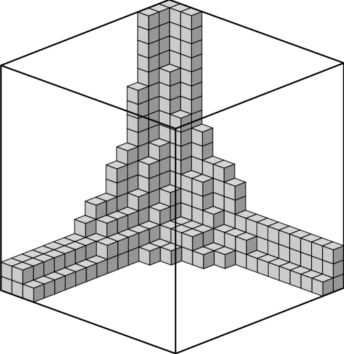
Figure 4: A 3d partition ending on three given 2d partitions

Let $P_{N_{1},N_{2},N_{3}}(\lambda,\mu,\nu)$ be the partition function in which every $\pi$ is weighted by $q^{\textup{vol}(\pi)}$. It is obvious that the limit

$$P(\lambda,\mu,\nu)=\lim_{N_{1},N_{2},N_{3}\to\infty}q^{-N_{1}|\lambda|-N_{2}|\mu|-N_{3}|\nu|}P_{N_{1},N_{2},N_{3}}(\lambda,\mu,\nu)$$ (3.16)

exists as a formal power series in $q$. What should the relation of this to topological vertex be? From what we have said before this should be the topological vertex itself up to framing factors. Let us also fix the framing factor, to compare it to the canonical framing. First of all we need to multiply $P$ by

$$q^{{-1\over 2}(|\lambda|+|\mu|+|\nu|)}$$

This is related to our discussion of the gluing algorithm (of shifting $N_{i}\rightarrow N_{i}+{1\over 2}$) and splitting the point of gluing between the two vertices. Secondly this perpendicular slicing is not the same as canonical framing. We need to rotate the perpendicular slicing to become the canonical framing. This involves the rotation of the partition along its first column by one unit and the sense of the rotation is to increase the number of points. For each representation this gives

$${1\over 2}\sum_{i}\lambda_{i}(\lambda_{i}-1)={1\over 2}(\|\lambda\|^{2}-|\lambda|)$$

extra boxes which we have to subtract off and gives the additional weight. Here

$$\|\lambda\|^{2}=\sum\lambda_{i}^{2}\,.$$

Combining with the previous factor we get a net factor of

$$q^{{1\over 2}(||\lambda||^{2}+||\mu||^{2}+||\nu||^{2})}$$

Moreover we should normalize as usual by dividing by the partition function with trivial asymptotic partition, which is the McMahon function. We thus expect

$$\prod_{n}(1-q^{n})^{n}q^{{1\over 2}(||\lambda||^{2}+||\mu||^{2}+||\nu||^{2})}P(\lambda,\mu,\nu)=C(\lambda,\mu,\nu).$$

We will see below that this is true up to $g_{s}\rightarrow-g_{s}$ and an overall factor that does not affect the gluing properties of the vertex (as they come in pairs) and it can be viewed as a gauge choice for the topological vertex.

3.4.2 Transfer matrix formula

Recall that in the transfer matrix setup one slices the partition diagonally. Compared with the perpendicular cutting, the diagonal cutting adds extra boxes to the partition and, as a result, it increases its volume by $\binom{\lambda}{2}+\binom{\mu^{t}}{2}$, where, by definition

$$\binom{\lambda}{2}=\sum_{i}\binom{\lambda_{i}}{2}\,.$$ (3.17)

Also, for the transfer-matrix method it is convenient to let $N_{3}=\infty$ from the very beginning, that is, to consider

$$P_{N_{1},N_{2}}(\lambda,\mu,\nu)=\lim_{N_{3}\to\infty}q^{-N_{3}|\nu|}P_{N_{1},N_{2},N_{3}}(\lambda,\mu,\nu)\,.$$ (3.18)

The partition function $P_{N_{1},N_{2}}(\lambda,\mu,\nu)$ counts 3d partitions $\pi$ with given boundary conditions on the planes $x_{1,2}=N_{1,2}$ inside the container which is a semiinfinite cylinder with base

$$[0,N_{1}]\times[0,N_{2}]\setminus\nu\,,$$

see Figure 5. In other words, $P_{N_{1},N_{2}}(\lambda,\mu,\nu)$ counts skew 3d partitions in the sense of [16].

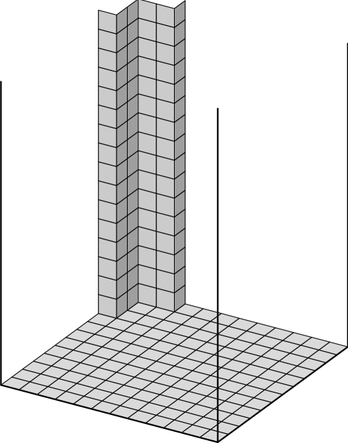
Figure 5: The container for skew 3d partitions

The main observation about skew 3d partitions is that their diagonal slices interlace in the pattern dictated by the shape $\nu$. This gives the following transfer-matrix formula for (3.18), which is a direct generalization of (3.4):

$$P_{N_{1},N_{2}}(\lambda,\mu,\nu)=q^{-\binom{\lambda}{2}-\binom{\mu^{t}}{2}}\,\times\\ \left\langle\lambda^{t}\left|\left(\prod_{\begin{subarray}{c}N_{1}-1\\ \textup{terms}\end{subarray}}q^{L_{0}}\,\Gamma_{\pm}(1)\right)q^{L_{0}}\left(\prod_{\begin{subarray}{c}N_{2}-1\\ \textup{terms}\end{subarray}}\Gamma_{\pm}(1)\,q^{L_{0}}\right)\right|\mu\right\rangle\,,$$ (3.19)

where the pattern of pluses and minuses in $\Gamma_{\pm}$ is dictated by the shape of $\nu$.

3.4.3 Transformation of the operator formula

Now we apply to the formula (3.19) the following three transformations:

• Commute the operators $q^{L_{0}}$ to the outside, splitting the middle one in half. The operators $\Gamma_{\pm}(1)$ will be conjugated to the operators $\Gamma_{\pm}(q^{\dots})$ in the process.

• Commute the raising operators $\Gamma_{-}$ to the left and the lowering operators $\Gamma_{+}$ to the right. There will be some overall, $\nu$-dependent multiplicative factor $Z(\nu)$ from this operation.

• Write the resulting expression as a sum over intermediate states $|\eta\rangle\langle\eta|$.

3.4.4 The result

We obtain

$$P(\lambda,\mu,\nu)=Z(\nu)\,q^{-\binom{\lambda}{2}-\binom{\mu^{t}}{2}-|\lambda|/2-|\mu|/2}\,\sum_{\eta}s_{\lambda^{t}/\eta}(q^{-\nu-\rho})\,s_{\mu/\eta}(q^{-\nu^{t}-\rho})\,.$$ (3.20)

In order to determine the multiplicative factor $Z(\nu)$, we compute

$$P(\emptyset,\emptyset,\nu)=P(\nu,\emptyset,\emptyset)$$

using the formula (3.20). We get

$$Z(\nu)=\frac{q^{-\binom{\nu}{2}-|\nu|/2}\,s_{\nu^{t}}(q^{-\rho})}{\prod_{n>0}(1-q^{n})^{n}}\,.$$ (3.21)

Since

$$\frac{\kappa(\mu)}{2}=\binom{\mu}{2}-\binom{\mu^{t}}{2}\,,$$ (3.22)

comparing (3.20) with (3.15) we obtain

$$\boxed{C(\lambda,\mu,\nu;1/q)=q^{\frac{\|\lambda^{t}\|+\|\mu^{t}\|+\|\nu^{t}\|}{2}}\,\prod_{n>0}(1-q^{n})^{n}\,P(\lambda,\mu,\nu)\quad}$$ (3.23)

where

$$\frac{\|\lambda\|^{2}}{2}=\sum_{i}\frac{\lambda_{i}^{2}}{2}=\binom{\lambda}{2}+\frac{|\lambda|}{2}\,.$$ (3.24)

This is exactly what we aimed for, see Section 3.4.1, up to the following immaterial details. The difference between $\|\lambda^{t}\|$ and $\|\lambda\|$ is irrelevant since the gluing formula pairs $\lambda$ with $\lambda^{t}$. Also, since the string amplitudes are even functions of $g_{s}$, they are unaffected by the substitution $q\mapsto 1/q$. These differences can be viewed as a gauge choice for the topological vertex.

3.5 Other generalizations

One can use the topological vertex to glue various local ${\bf C^{3}}$ patches and obtain the topological A-model amplitudes. Thus it is natural to expect that there is a natural lattice model. There is a natural lattice [26] for the crystal in this case, obtained by viewing the Kähler form divided by $g_{s}$ as defining the first Chern class of a line bundle and identifying the lattice model with holomorphic sections of this bundle. This is nothing but geometric quantization of Calabi-Yau with the Kähler form playing the role of symplectic structure and $g_{s}$ playing the role of $\hbar$. The precise definition of lattice melting problem for this class is currently under investigation [26]. The fact that we have already seen the emergence of topological vertex in the lattice computation corresponding to ${\bf C}^{3}$ one would expect that asymptotic gluings suitably defined should give the gluing rules of the statistical mechanical model. It is natural to expect this idea also works the same way in the compact case, by viewing the Calabi-Yau as a non-commutative manifold with non-commutativity parameter being $g_{s}k$, where $k$ is the Kähler form.

It is also natural to embed this in superstring (this is currently under investigation [27]), where $g_{s}$ will be replaced by graviphoton field strength. The large $g_{s}$ in this context translates to strong graviphoton field strength, for which it is natural to expect discretization of spacetime. This is exciting as it will potentially give a novel realization of superstring target space as a discrete lattice.

4 Periodic dimers and toric local CY

4.1 Dimers on a periodic planar bipartite graph

A natural generalization of the ideas discussed here is the planar dimer model, see [19] for an introduction. Let $\Gamma$ be a planar graph (“lattice”) which is periodic and bipartite. The first condition means that it is lifted from a finite graph in the torus $\mathbf{T}^{2}$ via the standard covering map $\mathbf{R}^{2}\to\mathbf{T}^{2}$. The second condition means that the vertices of $\Gamma$ can be partitioned into two disjoint subsets (“black” and “white” vertices) such that edges connect only white vertices to black vertices. Examples of such graphs are the standard square or honeycomb lattices.

By definition, a dimer configuration on $\Gamma$ is a collection of edges $D=\{e\}$ such that every vertex is incident to exactly one edge in $D$. Subject to suitable boundary conditions, the partition function of the dimer model is defined by

$$Z=\sum_{D}\prod_{e\in D}w(e)\,,$$

where $w(e)$ is a certain (Boltzmann) weight assigned to a given edge. For example, one can take both weights and boundary conditions to be periodic, in which case $Z$ is a finite sum. One can also impose boundary conditions at infinity by saying that the dimer configuration should coincide with a given configuration outside some ball of a large radius. The relative weight of such a configuration is a well-defined finite product, but the sum $Z$ itself is infinite. In order to make it convergent, one introduces a factor of $q^{\textup{volume}(D)}$, defined in terms of the height function, see below. Other boundary conditions can be given by cutting a large but finite piece out of the graph $\Gamma$ and considering dimers on it.

Simple dimer models, such as equal weight square or honeycomb grid dimer models with simple boundary conditions were first considered in the physics literature many years ago [20, 21]. A complete theory of the dimer model on a periodic weighted planar bipartite graph was developed in [24, 25]. It has some distinctive new features due to spectral curve being a general high genus algebraic curve. We will now quote some results of [24, 25] and indicate their relevance in our setting.

4.2 Periodic configurations and spectral curve

Consider dimer configuration $D$ on a torus or, equivalently, a dimer configuration in the plane that repeat periodically, like a wall-paper pattern. There are finitely many such configurations and they will play a special role for us, namely they will describe the possible facets of our CY crystal. We will now introduce a certain refined counting of these configurations.

Given two configurations $D_{1}$ and $D_{2}$ on a torus $\mathbf{T}^{2}$, their union is a collection of closed loops on $\mathbf{T}^{2}$. These loops come with a natural orientation by, for example, going from white to black vertices along the edges of the first dimer and from black to white vertices along the edges of the second dimer. Hence, they define an element (by summing over all classes of the loops)

$$h=(h_{1},h_{2})\in H_{1}(\mathbf{T}^{2},\mathbf{Z})\,,$$

of the first homology group of the torus. Fixing any configuration $D_{0}$ as our reference point, we can associate $h=h(D)$ to any other dimer configuration and define

$$F(z,w)=\sum_{D}(-1)^{Q(h)}\,z^{h_{1}}\,w^{h_{2}}\,\prod_{e\in D}w(e)\,,$$ (4.25)

where $Q(h)$ is any of the 4 theta-characteristic, for example, $Q((h_{1},h_{2}))=h_{1}h_{2}$. The ambiguity in the definition of (4.25) comes from the choice of the reference dimer $D_{0}$, which means overall multiplication by a monomial in $z$ and $w$, the choice of the basis for $H_{1}(\mathbf{T}^{2},\mathbf{Z})$, which means $SL(2,\mathbf{Z})$ action, and the choice of the theta-characteristic, which means flipping the signs of $z$ and $w$.

The locus $F(z,w)=0$ defines a curve in the toric surface corresponding to the Newton polygon of $F$. It is called the spectral curve of the dimer problem for the given set of weights. It is the spectral curve of the Kasteleyn operator on $\Gamma$, the variables $z$ and $w$ being the Bloch-Floquet multipliers in the two directions. In our situation, the curve $F(z,w)$ will be related to the mirror Calabi-Yau threefold.

4.3 Height function and “empty” configurations

Now consider dimer configurations in the plane. The union of two dimer configurations $D_{1}$ and $D_{2}$ again defines a collection of closed oriented loops. We can view it as the boundary of the level sets of a function $h$, defined on the cells (a.k.a. faces) of the graph $\Gamma$. This function $h$ is well-defined up to a constant and is known as the height function.

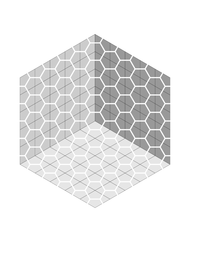
Figure 6: The “Empty room” configuration of honeycomb dimers

It is instructive to see how for dimers on the hexagonal lattice this reproduces the combinatorics of the 3d partitions, the height function giving the previously missing 3rd spatial coordinate, see Figure 6. The “full corner” or “empty room” configuration, which was our starting configuration describing the fully quantum $\mathbf{C}^{3}$ in the language of the dimers becomes the unique, up-to translation, configuration in which the periodic dimer patterns can come together. Each rhombus corresponds to one dimer (the edge of the honeycomb lattice inside it).

For general dimers, there are many periodic dimer patterns and there are (integer) moduli in how they can come together. For example, for the square lattice, which is the case corresponding to the $\mathcal{O}(-1)\oplus\mathcal{O}(-1)\rightarrow\mathbf{P}^{1}$ geometry, the periodic patterns are the brickwall patterns and there is one integer degree of freedom in how they can be patched together. One possible such configuration is shown in Figure 7. The arrows in Figure 7 point from white vertices to black ones to help visualize the difference between the 4 periodic patterns.

All of these “empty” configurations can serve as the initial configuration, describing the fully quantum toric threefold, for the dimer problem. When lifted in 3d via the height function, each empty configuration follows a piece-wise linear function, which is the boundary of the polyhedron defining the toric variety. In particular, the number of “empty room” moduli matches the Kähler moduli of the toric threefold and changes in its combinatorics correspond to the flops.

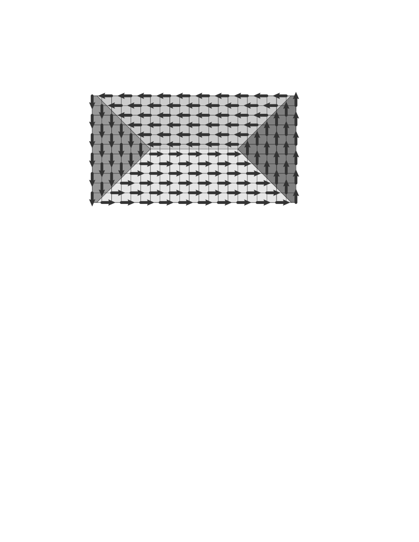
Figure 7: An “Empty room” configuration of square dimers

Readers familiar with $(p,q)$ 5-brane webs [22] and their relation to toric Calabi-Yau [23] immediately see a dictionary: A 5-brane configuration is identified as the transition line from one rigid dimer configuration to other, which in toric language is related to which $\mathbf{T}^{2}$ cycle of Calabi-Yau shrinks over it. For example the the $\mathbf{C}^{3}$ geometry is mapped to three 5-branes (of types $(1,0),(0,1),(-1,-1)$) on the 2 plane meeting at a point where each region gets identified with a particular dimer configuration. Similar description holds for arbitrary 5-brane webs. In this context the $F(z,w)=F(e^{-u},e^{-v})$ is identified with the mirror geometry [13].

4.4 Excitations and limit shape

Now we can start “removing atoms” from the “full crystal” configuration, adding the cost of $q$ to each increase in the height function. The limit shape that develops, is controlled by the surface tension of the dimer problem. This is a function of a slope measuring how much the dimer likes to have height function with this slope. Formally, it is defined as the $n\to\infty$ limit of the free energy per fundamental domain for dimer configurations on the $n\times n$ torus $\mathbf{T}^{2}$ restricted to lie in a given homology class or, equivalently, restricted to have certain slope when lifted to a periodic configuration in the plane.

One of the main results of [24] is the identification of this function with the Legendre dual of the Ronkin function of the polynomial (4.25) defined by

$$R(U,V)=\frac{1}{4\pi^{2}}\iint_{0}^{2\pi}\log\,|F(U+i\theta,V+i\phi)|\,d\theta d\phi\,.$$ (4.26)

The Wulff construction implies that the Ronkin function itself is one of the possible limit shapes, the one corresponding to its own boundary conditions. Note that this is exactly what one would anticipate from our general conjecture if we view $F(z,w)$ as the describing the mirror geometry. In fact following the same type of argument as in the ${\bf C}^{3}$ case discussed before, would lead us to the above Ronkin function.

As an example consider the dimers on the hexagonal lattice with $1\times 1$ fundamental domain. In this case the edge weights can be gauged away and (4.26) becomes the Ronkin function considered in Section 2.2. For the square lattice with $1\times 1$ fundamental domain, there is 1 gauge invariant combination of the 4 weights and the spectral curve takes the form

$$F(z,w)=1+z+w-e^{-t}zw\,,$$

where $t$ is a parameter related to the size of $\mathbf{P}^{1}$ in the $\mathcal{O}(-1)\oplus\mathcal{O}(-1)\rightarrow\mathbf{P}^{1}$ geometry. The spectral curve is a hyperbola in $\mathbf{C}^{2}$ and (the negative of) its Ronkin function is plotted in Figure 8. Note how one can actually see the projection of the mirror curve !

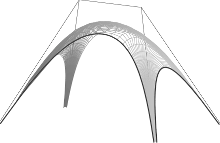
Figure 8: The Ronkin function of a hyperbola

All possible limit shapes for given set of dimer weights are maximizers of the surface tension functional and in this sense are very similar to minimal surfaces. An analog of the Weierstraß parameterization for them in terms of analytic data was found in [25]. It reduces the solution of the Euler-Lagrange PDE’s to solving equations for finitely many parameters, essentially finding a plane curve of given degree and genus satisfying certain tangency and periods conditions.

In the limit of extreme weights and large initial configurations, the amoebas and Ronkin functions degenerate to the piecewise-linear toric geometry. In this limit, it is possible to adjust parameters to reproduce the topological vertex formula for the GW invariants of the toric target obtained in [1]. We expect that the general case will reproduce the features of the background dependence (i.e. holomorphic anomaly) in the A-model [10]. This issue is presently under investigation [28].

Acknowledgments

We would like to thank the Simons workshop in Mathematics and Physics at Stony Brook for a very lively atmosphere which directly led to this work. We would also like to thank M. Aganagic, R. Dijkgraaf, S. Gukov, A. Iqbal, S. Katz, A. Klemm, M. Marino, N. Nekrasov, H. Ooguri, M. Rocek, G. Sterman and A. Strominger for valuable discussions. We thank J. Zhou for pointing out an inaccuracy in the formula (3.15) in the first version of this paper.

A. O. was partially supported by DMS-0096246 and fellowships from the Packard foundation. N. R. was partially supported by the NSF grant DMS-0307599. The research of C.V. is supported in part by NSF grants PHY-9802709 and DMS-0074329.

References

- [1] M. Aganagic, A. Klemm, M. Marino and C. Vafa, arXiv:hep-th/0305132; M. Aganagic, R. Dijkgraaf, A. Klemm, M. Marino and C. Vafa, to appear.
- [2] A. Iqbal, arXiv:hep-th/0207114.
- [3] D. E. Diaconescu and B. Florea, arXiv:hep-th/0309143.
- [4] S. Katz, A. Klemm and C. Vafa, Nucl. Phys. B 497 (1997) 173 [arXiv:hep-th/9609239]; S. Katz, P. Mayr and C. Vafa, Adv. Theor. Math. Phys. 1, 53 (1998) [arXiv:hep-th/9706110].
- [5] N. Nekrasov and A. Okounkov, arXiv:hep-th/0306238.
- [6] A. Iqbal and A. K. Kashani-Poor, arXiv:hep-th/0306032.
- [7] A. Okounkov and R. Pandharipande, math.AG/0204305, math.AG/0207233, math.AG/0308097.
- [8] C.-C. M. Liu, K. Liu, J. Zhou, math.AG/0306257, math.AG/0306434, math.AG/0308015.
- [9] A. Okounkov and R. Pandharipande, math.AG/0307209.
- [10] M. Bershadsky, S. Cecotti, H. Ooguri and C. Vafa, Commun. Math. Phys. 165, 311 (1994) [arXiv:hep-th/9309140].
- [11] R. Gopakumar and C. Vafa, arXiv:hep-th/9809187.
- [12] C. Faber and R. Pandharipande, arXiv:math.ag/0002112.
- [13] K. Hori and C. Vafa, arXiv:hep-th/0002222.
- [14] K. Hori, A. Iqbal and C. Vafa, arXiv:hep-th/0005247.
- [15] R. Cerf and R. Kenyon, Comm. Math. Phys. 222 (2001), no. 1, 147–179.
-
[16]
A. Okounkov and N. Reshetikhin,
Journal of the American Mathematical Society,
16, n.3(2003), pp.581-603,
and the paper to appear. - [17] I. G. Macdonald, Symmetric functions and Hall polynomials, Clarendon Press, 1995.
- [18] V. Kac Infinite-dimensional Lie algebras, Cambridge University Press, 1990.
- [19] R. Kenyon, An introduction to the dimer model, available from http://topo.math.u-psud.fr/kenyon/papers/papers.html
- [20] P. W. Kasteleyn, Physica 27 (1961) 1209–1225.
- [21] M. Fisher and H. Temperley, Phil Mag. 6 (1961) 1061–1063.
- [22] O. Aharony, A. Hanany and B. Kol, JHEP 9801, 002 (1998) [arXiv:hep-th/9710116].
- [23] N. C. Leung and C. Vafa, Adv. Theor. Math. Phys. 2, 91 (1998) [arXiv:hep-th/9711013].
- [24] R. Kenyon, A. Okounkov, and S. Sheffield, Dimers and amoebae, to appear.
- [25] R. Kenyon and A. Okounkov, to appear.
- [26] A. Iqbal, N. Nekrasov, A. Okounkov and C. Vafa, work in progress.
- [27] H. Ooguri, A. Strominger and C. Vafa, work in progress.
- [28] R. Kenyon, A. Okounkov, and C. Vafa, work in progress.