Conformal field theories in random domains
and Stochastic Loewner evolutions.

Abstract

We review the recently developed relation between the traditionnal algebraic approach to conformal field theories and the more recent probabilistic approach based on stochastic Loewner evolutions. It is based on implementing random conformal maps in conformal field theories.

1 Introduction.

Fractal critical clusters are hallmarks of criticality, as it may be illustrated by considering the $Q$-state Potts models whose lattice partition functions are:

$$Z=\sum_{\{s({\bf r})\}}\ \exp[\,J\sum_{{\bf r}\sqcup{\bf r^{\prime}}}\delta_{s({\bf r}),s({\bf r^{\prime}})}\,]$$

The sum is over all spin configurations and ${\bf r}\sqcup{\bf r^{\prime}}$ refers to neighbor sites ${\bf r}$ and ${\bf r^{\prime}}$ on the lattice. The spin $s({\bf r})$ takes $Q$ possible values. By expanding the exponential factor using $\exp[J(\delta_{s({\bf r}),s({\bf r^{\prime}})}-1)]=(1-p)+p\delta_{s({\bf r}),s({\bf r^{\prime}})}$ with $p=1-e^{-J}$, these partition functions may be rewritten as sums over cluster configurations

$$Z=e^{JL}\ \sum_{C}\,p^{\|C\|}\,(1-p)^{L-\|C\|}\,Q^{N_{C}}$$

where $L$ is the number of links of the lattice, $N_{C}$ the number of clusters in the configuration $C$ and $\|C\|$ the number of links inside the $N_{C}$ clusters, usually called FK-clusters. Criticality is then encoded in the fractal nature of these clusters.

The stochastic Loewner evolutions (SLE) [2] are mathematically well-defined processes describing the growth of random sets, called the SLE hulls, and of random curves, called the SLE traces, embedded in the two-dimensional plane. The growths of these sets are encoded into families of random conformal maps satisfying specific evolution equations. Their distribution depends on a real parameter $\kappa$.

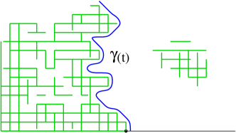
Figure 1: A FK-cluster configuration in the Potts model. The SLE trace is the boundary of the FK-cluster connected to the negative real line.

The connexion between critical systems and SLE growths may intuitively be undertsood as follows: imagine considering the $Q$-state Potts models on a lattice covering the upper half plane with boundary conditions on the real line such that all spins on the negative real axis are frozen to the same identical value while spins on the right of the origin are free with non assigned values. Then, in each configuration there exists a FK-cluster growing from the negative half real axis into the upper half plane whose boundary starts at the origin. In the continuum limit, this boundary curve is conjectured to be statistically equivalent to a SLE trace. The SLE parameter $\kappa$ is linked to the Potts parameter by $Q=4\cos^{2}(\frac{4\pi}{\kappa})$, with $\kappa\geq 4$. See Figure (1).

The aim of this note is to described a precise connexion, which we have developed in refs.[5, 6, 7], between the traditionnal algebraic approach to conformal field theories and the probabilistic approach based on stochastic Loewner evolutions. The main point consists in considering conformal field theories on random domains defined as the complements of the growing random SLE hulls. Although we illustrate this connexion using the chordal version of SLE, we shall also touch upon the generalization to the radial SLE.

2 (Chordal) stochastic Loewner evolutions.

Given a simply connected domain $\mathbb{U}$ in the complex plane, stochastic Loewner evolutions (SLE) describe the growth of random curves emerging from the boundary of $\mathbb{U}$. There are two cases depending whether these curves connect two points on the boundary $\partial\mathbb{U}$ (for the chordal SLE), or one point on the boundary and one in the bulk of $\mathbb{U}$ (for the radial SLE). We shall mainly deal with the chordal case, except in the last section.

To be more precise, let a hull in the upper half plane $\mathbb{H}=\{z\in\mathbb{C},\Im{\rm m}\,z>0\}$ be a bounded subset $\mathbb{K}\subset\mathbb{H}$ such that $\mathbb{H}\setminus\mathbb{K}$ is open, connected and simply connected.

The local growth of a family of hulls $\mathbb{K}_{t}$ parametrized by $t\in[0,T[$ with $\mathbb{K}_{0}=\emptyset$ is related to complex analysis as follows. By the Riemann mapping theorem, $\mathbb{H}_{t}\equiv\mathbb{H}\setminus\mathbb{K}_{t}$, the complement of $\mathbb{K}_{t}$ in $\mathbb{H}$, which is simply connected by hypothesis, is conformally equivalent to $\mathbb{H}$ via a map $f_{t}$. This map can be normalized to behave as $f_{t}(z)=z+2t/z+O(1/z^{2})$, using the $PSL_{2}(\mathbb{R})$ automorphism group of $\mathbb{H}$. The crucial condition of local growth leads to the Loewner differential equation

$$\partial_{t}f_{t}(z)=\frac{2}{f_{t}(z)-\xi_{t}}\ ,\quad f_{t=0}(z)=z$$ (1)

with $\xi_{t}$ a real function. For fixed $z$, $f_{t}(z)$ is well-defined up to the time $\tau_{z}$ for which $f_{\tau_{z}}(z)=\xi_{\tau_{z}}$.

(Chordal) stochastic Loewner evolutions is obtained [2] by choosing $\xi_{t}=\sqrt{\kappa}\,B_{t}$ with $B_{t}$ a normalized Brownian motion and $\kappa$ a real positive parameter so that $\mathbb{E}[\xi_{t}\,\xi_{s}]=\kappa\,{\rm min}(t,s)$. The SLE hull is reconstructed from $f_{t}$ by $\mathbb{K}_{t}=\{z\in{\mathbb{H}}:\ \tau_{z}\leq t\}$ and the SLE trace $\gamma_{[0,t]}$ by $\gamma(t)=\lim_{\epsilon\to 0^{+}}f_{t}^{-1}(\xi_{t}+i\epsilon)$. Basic properties of the SLE hulls and SLE traces are described in [2, 3, 4]. In particular, $\gamma_{[0,t]}$ is almost surely a curve. It is non-self intersecting and it coincides with $\mathbb{K}_{t}$ for $0<\kappa\leq 4$, while for $4<\kappa<8$ it possesses double-points and it does not coincide with $\mathbb{K}_{t}$.

For establishing contact with conformal field theories (CFT), it is useful to define $k_{t}(z)\equiv f_{t}(z)-\xi_{t}$ which satisfies the stochastic differential equation

$$dk_{t}=\frac{2dt}{k_{t}}-d\xi_{t}.$$

The conditions at spatial infinity satisfied by $k_{t}$ imply that its germ there belongs to the group $N_{-}$ of germs of holomorphic functions at $\infty$ of the form $z+\sum_{m\leq-1}f_{m}z^{m+1}$. The group $N_{-}$ acts on itself by composition, $\gamma_{f}\cdot F\equiv F\circ f$ for $f\in N_{-}$, and $\gamma_{g\circ f}=\gamma_{f}\cdot\gamma_{g}$. In particular, to $k_{t}$ we can associate $\gamma_{k_{t}}\in N_{-}$, which satisfy, by Itô’s formula:

$$d\gamma_{k_{t}}\cdot F=(\gamma_{k_{t}}\cdot F^{\prime})(\frac{2dt}{k_{t}}-d\xi_{t})+\frac{\kappa}{2}(\gamma_{k_{t}}\cdot F^{\prime\prime})$$

Alternatively, this may be read as:

$$\gamma_{k_{t}}^{-1}\cdot d\gamma_{k_{t}}=dt(\frac{2}{z}\partial_{z}+\frac{\kappa}{2}\partial_{z}^{2})-d\xi_{t}\partial_{z}.$$ (2)

The operators $l_{n}=-z^{n+1}\partial_{z}$ are represented in conformal field theories by operators $L_{n}$ which satisfy the Virasoro algebra $\mathfrak{vir}$ :

$$[L_{n},L_{m}]=(n-m)L_{n+m}+\frac{c}{12}(n^{3}-n)\delta_{n+m,0}\qquad[c,L_{n}]=0.$$

The representations of $\mathfrak{vir}$ are not automatically representations of $N_{-}$, one of the reasons being that the Lie algebra of $N_{-}$ contains infinite linear combinations of the $l_{n}$’s. However, as we shall explain in the next section, highest weight representations of $\mathfrak{vir}$ can be extended in such a way that $N_{-}$ get embedded in a appropriate completion $\overline{\mathcal{U}(\mathfrak{n}_{-})}$ of the enveloping algebra of some subalgebra $\mathfrak{n}_{-}$ of $\mathfrak{vir}$. This will allows us to associate to any $\gamma_{f}\in N_{-}$ an operator $G_{f}$ acting on appropriate representations of $\mathfrak{vir}$ and satisfying $G_{g\circ f}=G_{f}G_{g}$. Implementing this construction to $k_{t}$ yields random operators $G_{k_{t}}\in\overline{\mathcal{U}(\mathfrak{n}_{-})}$ which satisfy the stochastic Itô equation:

$$G_{k_{t}}^{-1}dG_{k_{t}}=dt(-2L_{-2}+\frac{\kappa}{2}L_{-1}^{2})+d\xi_{t}L_{-1}.$$ (3)

Compare with eq.(2). This may be viewed as defining a Markov process in $\overline{\mathcal{U}(\mathfrak{n}_{-})}$.

Since $G_{k_{t}}$ turn out to be the operators intertwining the conformal field theories in $\mathbb{H}$ and in the random domains $\mathbb{H}_{t}$, the basic observation which allows us to couple CFTs to SLEs is the following [5]:

Let $|\omega\rangle$ be the highest weight vector in the irreducible highest weight representation of $\mathfrak{vir}$ of central charge $c_{\kappa}=\frac{(6-\kappa)(3\kappa-8)}{2\kappa}$ and conformal weight $h_{\kappa}\equiv h_{1;2}=\frac{6-\kappa}{2\kappa}$.
Then $\mathbb{E}[G_{k_{t}}|\omega\rangle|\{G_{k_{u}}\}_{u\leq s}]$ is time independent for $t\geq s$ and:

$$\mathbb{E}[\,G_{k_{t}}|\omega\rangle\,|\{G_{k_{u}}\}_{u\leq s}]=G_{k_{s}}|\omega\rangle$$ (4)

This result is a direct consequence of eq.(3) and the null vector relation $(-2L_{-2}+\frac{\kappa}{2}L_{-1}^{2})|\omega\rangle=0$ so that $dG_{k_{t}}|\omega\rangle=G_{k_{t}}L_{-1}|\omega\rangle d\xi_{t}$.

This result has the following consequences. Consider CFT correlation functions in $\mathbb{H}_{t}$. They can be computed by looking at the same theory in $\mathbb{H}$ modulo the insertion of an operator representing the deformation from $\mathbb{H}$ to $\mathbb{H}_{t}$, see the next section. This operator is $G_{k_{t}}$. Suppose that the central charge is $c_{\kappa}$ and the boundary conditions are such that there is a boundary changing primary operator of weight $h_{\kappa}$ inserted at the tip of $\mathbb{K}_{t}$. Then in average the correlation functions of the conformal field theory in the fluctuating geometry $\mathbb{H}_{t}$ are time independent and equal to their value at $t=0$.

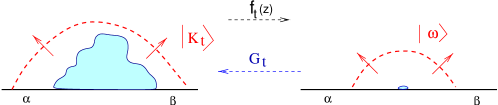
Figure 2: A representation of the boundary hull state and of the map intertwining different formulations of the CFT.

The state $G_{k_{t}}|\omega\rangle$ may be interpreted as follows. Imagine defining the conformal field theory in $\mathbb{H}_{t}$ via a radial quantization, so that the conformal Hilbert spaces are defined over curves topologically equivalent to half circles around the origin. Then, the SLE hulls manifest themselves as disturbances localized around the origin, and as such they generate states in the conformal Hilbert spaces. Since, $G_{k_{t}}$ intertwines the CFT in $\mathbb{H}$ and in $\mathbb{H}_{t}$, these states are $G_{k_{t}}|\omega\rangle$ with $|\omega\rangle$ keeping track of the boundary conditions. See Figure (2).

3 Conformal transformations in CFT and applications.

The basic principles of conformal field theory state that correlation functions in a domain $\mathbb{U}$ are known once they are known in a domain $\mathbb{U}_{0}$ and an explicit conformal map $f$ from $\mathbb{U}$ to $\mathbb{U}_{0}$ preserving boundary conditions is given. Primary fields have a very simple behavior under conformal transformations: for a bulk primary field $\varphi$ of weight $(h,\overline{h})$, $\varphi(z,\overline{z})dz^{h}d\overline{z}^{\overline{h}}$ is invariant, and for a boundary conformal field $\psi$ of weight $\delta$, $\psi(x)|dx|^{\delta}$ is invariant. Their statistical correlations in $\mathbb{U}$ and $\mathbb{U}_{0}$ are related by

$$\langle\cdots\varphi(z,\overline{z})\cdots\psi(x)\cdots\rangle_{\mathbb{U}}=\langle\cdots\varphi(f(z),\overline{f(z)})f^{\prime}(z)^{h}\overline{f^{\prime}(z)}^{\overline{h}}\cdots\psi(f(x))|f^{\prime}(x)|^{\delta}\cdots\rangle_{\mathbb{U}_{0}}.$$ (5)

Infinitesimal deformations of the underlying geometry are implemented in local field theories by insertions of the stress-tensor. In conformal field theories, the stress-tensor is traceless so that it has only two independent components, one of which, $T(z)$, is holomorphic (except for possible singularities when its argument approaches the arguments of other inserted operators). The field $T(z)$ itself is not a primary field but a projective connection,

$$\langle\cdots T(z)\cdots\rangle_{\mathbb{U}}=\langle\cdots T(f(z))f^{\prime}(z)^{2}+\frac{c}{12}\mathrm{S}f(z)\cdots\rangle_{\mathbb{U}_{0}},$$

with $c$ is the CFT central charge and $\mathrm{S}f(z)=\left(\frac{f^{\prime\prime}(z)}{f^{\prime}(z)}\right)^{\prime}-\frac{1}{2}\left(\frac{f^{\prime\prime}(z)}{f^{\prime}(z)}\right)^{2}$ the Schwartzian derivative of $f$ at $z$.

This applies to infinitesimal deformations of the upper half plane. Consider an infinitesimal hull $\mathbb{K}_{\epsilon;\mu}$, whose boundary is the curve $x\to\epsilon\,\pi\mu(x)$, $x$ real and $\epsilon\ll 1$, so that $\mathbb{K}_{\epsilon;\mu}=\{z=x+iy\in\mathbb{H},\ 0<y<\epsilon\,\pi\mu(x)\}$. Assume for simplicity that $\mathbb{K}_{\epsilon;\mu}$ is bounded away from $0$ and $\infty$. Let $\mathbb{H}_{\epsilon;\mu}\equiv\mathbb{H}\setminus\mathbb{K}_{\epsilon;\mu}$. To first order in $\epsilon$, its uniformizing map onto $\mathbb{H}$ is

$$z+\epsilon\,\int_{\mathbb{R}}\frac{\mu(y)dy}{z-y}+o(\epsilon).$$

To first order in $\epsilon$, correlation functions in $\mathbb{H}_{\epsilon;\mu}$ are related to those in $\mathbb{H}$ by insertion of $T$:

$$\frac{d}{d\epsilon}\langle\left(\cdots\varphi(z,\overline{z})\cdots\psi(x)\cdots\right)\rangle_{\mathbb{H}_{\epsilon;\mu}}|_{\epsilon=0^{+}}=\int_{\mathbb{R}}dy\mu(y)\,\langle T(y)\left(\cdots\varphi(z,\overline{z})\cdots\psi(x)\cdots\right)\rangle_{\mathbb{H}}$$ (6)

With the basic CFT relation [1] between the stress tensor and the Virasoro generators, $T(z)=\sum_{n}L_{n}z^{n-2}$, this indicates that infinitesimal deformations of the domains are described by insertions of elements of the Virasoro algebra.

Finite conformal transformations are implemented in conformal field theories by insertion of operators, representing some appropriate exponentiation of insertions of the stress tensor. Let $\mathbb{U}$ be conformally equivalent to the upper half plane $\mathbb{H}$ and $f$ the corresponding uniformazing map. Then, following [6], the finite conformal deformations that leads from the conformal field theory on $\mathbb{U}$ to that on $\mathbb{H}$ can be represented by an operator $G_{f}$:

$$\langle\cdots\varphi(z,\overline{z})\cdots\psi(x)\cdots\rangle_{\mathbb{U}}=\langle G_{f}^{-1}\left(\cdots{\varphi}(z,\overline{z})\cdots{\psi}(x)\cdots\right)G_{f}\rangle_{\mathbb{H}}.$$ (7)

This relates correlation functions in $\mathbb{U}$ to correlation functions in $\mathbb{H}$ where the field arguments are taken at the same point but conjugated by $G_{f}$. Radial quantization is implicitely asssumed in eq.(7). Compare with eq.(5).

The following is a summary, extracting the main steps, of a construction of $G_{f}$ described in details in [6]. To be more precise, we need to distinguish cases depending whether $f$ fixes the origin or the infinity. We also need a few simple definitions. We let $\mathfrak{vir}$ be the Virasoro algebra generated by the $L_{n}$ and $c$, and $\mathfrak{n}_{-}$ (resp. $\mathfrak{n}_{+}$) be the nilpotent Lie subalgebra of $\mathfrak{vir}$ generated by the $L_{n}$’s, $n<0$ (resp. $n>0$), and by $\mathfrak{b}_{-}$ (resp. $\mathfrak{b}_{+}$) the Borel Lie subalgebra of $\mathfrak{vir}$ generated by the $L_{n}$’s, $n\leq 0$ (resp $n\geq 0$) and $c$. We denote by $\overline{\mathcal{U}(\mathfrak{n}_{-})}$ (resp. $\overline{\mathcal{U}(\mathfrak{n}_{+})}$) appropriate completion of the enveloping algebra of $\mathfrak{n}_{-}$ (resp. $\mathfrak{n}_{+}$). We shall only consider highest weight vector representations of the Virasoro algebra.

$\bullet$ Finite deformations fixing $0$.

Let $N_{+}$ be the space of power series of the form $z+\sum_{m\geq 1}f_{m}z^{m+1}$ which have a non vanishing radius of convergence. With words, $N_{+}$ is the set of germs of holomorphic functions at the origin fixing the origin and whose derivative at the origin is $1$. In applications to the chordal SLE, we shall only need the case when the coefficients are real. But it is useful to consider the $f_{m}$’s as independent commuting indeterminates.

$N_{+}$ is a group for composition. Our aim is to construct a group (anti)-isomorphism from $N_{+}$ with composition onto a subset $\mathcal{N}_{+}\subset\overline{\mathcal{U}(\mathfrak{n}_{+})}$ with the associative algebra product.

We let $N_{+}$ act on $O_{0}$, the space of germs of holomorphic functions at the origin, by $\gamma_{f}\cdot F\equiv F\circ f$ for $f\in N_{+}$ and $F\in O_{0}$. This representation is faithful and $\gamma_{g\circ f}=\gamma_{f}\gamma_{g}$. We need to know how $\gamma_{f}$ varies when $f$ varies as $f\to f+\varepsilon v(f)$ for small $\varepsilon$ and an arbitrary vector field $v$. Taking $g=z+\varepsilon v(z)$ in the group law leads to $\gamma_{f+\varepsilon v(f)}F=\gamma_{f}\cdot F+\varepsilon\gamma_{f}\cdot(v\cdot F)+o(\varepsilon)$, where $v\cdot F(z)\equiv v(z)F^{\prime}(z)$ is the standard action of vector fields on functions. Using Lagrange inversion formula to determine the vector field $v$ corresponding to the variation of the indeterminate $f_{m}$ yields:

$$\gamma_{f}^{-1}\,\frac{\partial\gamma_{f}}{\partial f_{m}}=\sum_{n\geq m}\left(\oint_{0}\frac{dw}{2i\pi}w^{m+1}\frac{f^{\prime}(w)}{f(w)^{n+2}}\right)\,z^{n+1}\partial_{z}.$$

This system of first order partial differential equations makes sense in $\overline{\mathcal{U}(\mathfrak{n}_{+})}$ if we replace $l_{n}=-z^{n+1}\partial_{z}$ by $L_{n}$. So, we define a connection $A_{m}$ in $\overline{\mathcal{U}(\mathfrak{n}_{+})}$ by

$$A_{m}(f)\equiv\sum_{n\geq m}L_{n}\,\left(\oint_{0}\frac{dw}{2i\pi}w^{m+1}\frac{f^{\prime}(w)}{f(w)^{n+2}}\right)$$

which by construction satisfies the zero curvature condition, $\frac{\partial A_{l}}{\partial f_{k}}-\frac{\partial A_{k}}{\partial f_{l}}=[A_{k},A_{l}].$

We may thus construct an element $G_{f}\in\mathcal{N}_{+}\subset\overline{\mathcal{U}(\mathfrak{n}_{+})}$ for each $f\in N_{+}$ by solving the system

$$\frac{\partial G_{f}}{\partial f_{m}}=-G_{f}A_{m}(f),\qquad m\geq 1.$$ (8)

This system is guarantied to be compatible, because $N_{+}$ is convex and the representation of $N_{+}$ on $O_{0}$ is well defined for finite deformations $f$, faithful and solves the analogous system. The existence and unicity of $G_{f}$, with the initial condition $G_{f=z}=1$, is clear and the group (anti)-homomorphism property, $G_{f}G_{g}=G_{g\circ f}$, is true because it is true infinitesimally and $N_{+}$ is convex. To lowest orders: $G_{f}=1-f_{1}L_{1}+\frac{f_{1}^{2}}{2}(L_{1}^{2}+2L_{2})-f_{2}L_{2}+\cdots.$

The element $G_{f}$, acting on a highest weight representation of the Virasoro algebra, is the operator which implements the conformal map $f$ in conformal field theory. It acts on the stress tensor by conjugaison as:

$$G_{f}^{-1}T(z)G_{f}=T(f(z))f^{\prime}(z)^{2}+\frac{c}{12}Sf(z).$$ (9)

A formula which makes sense as long as $z$ is in the disk of convergence of $f(z)$ and $Sf(z)$, but which can be extended by analytic continuation if $f(z)$ allows it. A similar formula would hold if we would have consider the action of $G_{f}$ on local fields. In particular, by eq.(9), $G_{f}$ induces an homomorphism of the Virasoro algebra by $L_{m}\to L_{m}(f)\equiv G_{f}^{-1}L_{m}G_{f}$ with $G_{f}^{-1}T(z)G_{f}=\sum_{m}L_{m}(f)z^{-m-2}$:

$$G_{f}^{-1}L_{m}G_{f}=\frac{c}{12}\,\left(\oint_{0}\frac{dw}{2i\pi}w^{m+1}Sf(w)\right)+\sum_{n\geq m}L_{n}\,\left(\oint_{0}\frac{dw}{2i\pi}w^{m+1}\frac{f^{\prime}(w)^{2}}{f(w)^{n+2}}\right).$$

Eq.(8), which specifies the variations of $G_{f}$, can be rewritten in a maybe more familiar way involving the stress tensor. Namely, if $f$ is changed to $f+\delta f$ with $\delta f=\varepsilon v(f)$, then:

$$\delta G_{f}=-\varepsilon\,G_{f}\,\oint_{0}\frac{dz}{2i\pi}\,T(z)\,v(z).$$

If $v$ is not just a formal power series at the origin, but a convergent one in a neighborhood of the origin, we can freely deform contours in this formula, thus making contact with the infinitesimal deformations considered in eq.(6).

$\bullet$ Finite deformations fixing $\infty$.

All the previous considerations could be extended to the case in which the holomorphic functions fix $\infty$ instead of $0$. Let $N_{-}$ be the space of power series of the form $z+\sum_{m\leq-1}f_{m}z^{m+1}$ which have a non vanishing radius of convergence. We let it act on $O_{\infty}$, the space of germs of holomorphic functions at infinity, by $\gamma_{f}\cdot F\equiv F\circ f$. The adaptation of the previous computations shows that $\gamma_{f}^{-1}\frac{\partial\gamma_{f}}{\partial f_{m}}=\sum_{n\leq m}\left(\oint_{\infty}\frac{dw}{2i\pi}w^{m+1}\frac{f^{\prime}(w)}{f(w)^{n+2}}\right)z^{n+1}\partial_{z}.$ We transfer this relation to $\overline{\mathcal{U}(\mathfrak{n}_{-})}$ to define an (anti)-isomorphism from $N_{-}$ to $\mathcal{N}_{-}\subset\overline{\mathcal{U}(\mathfrak{n}_{-})}$ mapping $f$ to $G_{f}$ such that

$$\frac{\partial G_{f}}{\partial f_{m}}=-G_{f}\sum_{n\leq m}L_{n}\,\left(\oint_{\infty}\frac{dw}{2i\pi}w^{m+1}\frac{f^{\prime}(w)}{f(w)^{n+2}}\right),\qquad m\leq-1.$$

$\bullet$ Dilatations and translations.

We have been dealing with deformations around $0$ and $\infty$ that did not involve dilatation at the fixed point: $f^{\prime}(0)$ or $f^{\prime}(\infty)$ was unity. To gain some flexibility we may also authorize dilatations, say at the origin. The operator associated to a pure dilatation $z\to\lambda z$ is $\lambda^{-L_{0}}$. One can view a general $f$ fixing $0$ as the composition $f(z)=f^{\prime}(0)(z+\sum_{m}f_{m}z^{m+1})$ of a deformation at $0$ with derivative $1$ at $0$ followed by a dilatation, so that $G_{f}=G_{f/f^{\prime}(0)}\,f^{\prime}(0)^{-L_{0}}.$

We may also implement translations. Suppose that $f(z)=f^{\prime}(0)(z+\sum_{m}f_{m}z^{m+1})$ is a generic invertible germ of holomorphic function fixing the origin. If $a$ is in the interior of the disk of convergence of the power series expansion of $f$ and $f^{\prime}(a)\neq 0$, we may define a new germ $f_{a}(z)\equiv f(a+z)-f(a)$ with the same properties. The operators $G_{f}$ and $G_{f_{a}}$ implementing $f$ and $f_{a}$ are then related by $G_{f_{a}}=e^{-aL_{-1}}\,G_{f}\,e^{f(a)L_{-1}}.$

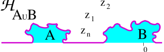
Figure 3: A typical two hull geometry.

$\bullet$ Finite deformations around $0$ and $\infty$.

Consider now a domain $\mathbb{H}_{A\cup B}$ of the type represented on fig.(3) which is the complement two disjoint hulls, the first one, say $A$, located around infinity but away from the origin, and the second one, say B, located around the origin and away from infinity. The uniformizing map $f_{A\cup B}$ of $\mathbb{H}_{A\cup B}$ onto $\mathbb{H}$ then does not exist at $0$ or at $\infty$.

However, in this situation, we may obtain the map $f_{A\cup B}$ by first removing $B$ by $f_{B}$, which is regular around $\infty$ and such that $f_{B}(z)=z+O(1)$ at infinity, and then $\widetilde{A}\equiv f_{B}(A)$ by $f_{\widetilde{A}}$ which is regular around $0$ and fixes $0$ ($f_{\widetilde{A}}^{\prime}(0)\neq 1$ is allowed). Of course, the roles of $A$ and $B$ could be interchanged, and we could first remove $A$ by $f_{A}$ which is regular around $0$ and fixes $0$ and then $\widetilde{B}\equiv f_{A}(B)$ by $f_{\widetilde{B}}$ which is regular around $\infty$ and such that $f_{\widetilde{B}}(z)=z+O(1)$.

Suppose that $f_{A}$ and $f_{B}$ are given. There is some freedom in the choice of $f_{\widetilde{A}}$ and $f_{\widetilde{B}}$ : namely we can replace $f_{\widetilde{A}}$ by $h_{0}\circ f_{\widetilde{A}}$ where $h_{0}\in PSL_{2}(\mathbb{R})$ fixing $0$, and $f_{\widetilde{B}}$ by $h_{\infty}\circ f_{\widetilde{B}}$ where $h_{\infty}\in PSL_{2}(\mathbb{R})$ such that $h_{\infty}(z)=z+O(1)$ at infinity, i.e. a translation. A simple computation shows that generically there is a unique choice of $f_{\widetilde{A}}$ and $f_{\widetilde{B}}$ such that $f_{\widetilde{B}}\circ f_{A}=f_{\widetilde{A}}\circ f_{B}$ and both equal to $f_{A\cup B}$.

For sufficiently disjoint hulls $A$ and $B$, as in fig.(3), there exists an open set such that for $z$ in this set, both $G^{-1}_{f_{\widetilde{A}}}\left(G^{-1}_{f_{B}}T(z)G_{f_{B}}\right)G_{f_{\widetilde{A}}}$ and $G^{-1}_{f_{\widetilde{B}}}\left(G^{-1}_{f_{A}}T(z)G_{f_{A}}\right)G_{f_{\widetilde{B}}}$ are well defined, given by absolutely convergent series, and are both equal to $T(f_{A\cup B}(z))f^{\prime}_{A\cup B}(z)^{2}+\frac{c}{12}Sf_{A\cup B}(z)$. As the modes $L_{n}$ of $T(z)$ generate all states in a highest weight representation, the operators $G_{f_{B}}G_{f_{\widetilde{A}}}$ and $G_{f_{A}}G_{f_{\widetilde{B}}}$ have to be proportional: they differ at most by a factor involving the central charge $c$. We write $G_{f_{B}}G_{f_{\widetilde{A}}}=Z(A,B)\;G_{f_{A}}G_{f_{\widetilde{B}}},$ or

$$G_{f_{A}}^{-1}\,G_{f_{B}}=Z(A,B)\,G_{f_{\widetilde{B}}}\,G_{f_{\widetilde{A}}}^{-1}.$$ (10)

Formula (10) plays for the Virasoro algebra the role that Wick’s theorem plays for collections of harmonic oscillators. Since $G_{f_{A}}$ and $G_{f_{\widetilde{A}}}$ belong to $\mathcal{N}_{+}$ while $G_{f_{B}}$ and $G_{f_{\widetilde{B}}}$ to $\mathcal{N}_{-}$, eq.(10) may also be viewed as defining a product between elements in $\mathcal{N}_{+}$ and $\mathcal{N}_{-}$. Note that $G_{f_{\widetilde{B}}}\,G_{f_{\widetilde{A}}}^{-1}$ is clearly well defined in highest weight vector representations of $\mathfrak{vir}$.

As implicit in the notation, $Z(A,B)$ depends only on $A$ and $B$: a simple computation shows that it is invariant if $f_{A}$ is replaced by $h_{0}\circ f_{A}$ and $f_{B}$ by $h_{\infty}\circ f_{B}$. It may be evaluated as follows. Let $A_{s}$ and $B_{t}$ be two families of hulls that interpolate between the trivial hull and $A$ or $B$ respectively and $f_{A_{s}}$ and $f_{B_{t}}$ be their uniformizing map. We arrange that $f_{A_{s}}$ and $f_{B_{t}}$ satisfy the genericity condition, so that unique $f_{A_{s,t}}$ and $f_{B_{t,s}}$ exist, which satisfy $f_{B_{t,s}}\circ f_{A_{s}}=f_{A_{s,t}}\circ f_{B_{t}}$. Define vector fields by $v_{A_{s}}$ and $v_{B_{t}}$ by $\frac{\partial f_{A_{s}}}{\partial s}=v_{A_{s}}(f_{A_{s}})$ and $\frac{\partial f_{B_{t}}}{\partial t}=v_{B_{t}}(f_{B_{t}})$. Then [6]:

$$\log Z(A_{\sigma},B_{\tau}) = \frac{c}{12}\int_{0}^{\sigma}ds\oint\frac{dw}{2i\pi}\;v_{A_{s}}(w)Sf_{B_{\tau,s}}(w)$$ (11)

$$= -\frac{c}{12}\int_{0}^{\tau}dt\oint\frac{dz}{2i\pi}\;v_{B_{t}}(z)Sf_{A_{\sigma,t}}(z).$$

$Z(A,B)$ may physically be interpreted as the interacting part of the CFT partition function in $\mathbb{H}\setminus(A\cup B)$.

This two hull construction may be used to define operators which are analogues of what vertex operators of dual models are for the Heisenberg algebra. Indeed, consider a hull $A$ whose closure does contain neither the origin nor the infinity. Let us pick the uniformizing map $f_{A}$ of its complement in $\mathbb{H}$ onto $\mathbb{H}$ which is regular both at the origin and at infinity and such that $f_{A}^{\prime}(0)=f_{A}^{\prime}(\infty)$. Since it is regular at the origin, we may implement $f_{A}$ in conformal field theory by $G_{A^{+}}\,f_{A}^{\prime}(0)^{-L_{0}}$ with $G_{A^{+}}$ in $\mathcal{N}_{+}$. Since it is also regular at infinity, we may alternatively implement it by $G_{A^{-}}\,f_{A}^{\prime}(\infty)^{-L_{0}}$ with $G_{A^{-}}\in\mathcal{N}_{-}$. The product

$$\mathcal{V}_{A}\equiv G_{A^{-}}\,G_{A^{+}}^{-1}$$

is well defined and non trivial in highest weight representation of $\mathfrak{vir}$. It may be thought of as the factorization of the identity since the conformal transformation it implements is the composition of two inverse conformal maps.

4 Virasoro representations.

The above formula may be used to define generalized coherent state representations of $\mathfrak{vir}$. The key point is to interpret the ‘Virasoro Wick theorem’, eq.(10), as defining an action of $\mathfrak{vir}$ on $\mathcal{N}_{-}$. This is a reformulation of a construction à la Borel-Weil presented in ref.[7].

$\bullet$ Representations around infinity.

Consider a Verma module $V(c,h)$ and take $x\neq 0$ its highest weight vector. Let $f=z+\sum_{m\leq-1}f_{m}z^{m+1}\in N_{-}$ and $G_{f}$ be the corresponding element in $\mathcal{N}_{-}$. The space $\{P_{y}[f]\equiv\left<y,G_{f}x\right>,y\in V(c,h)^{*}\}$, or $\{Q_{y}[f]\equiv\langle y,G_{f}^{-1}x\rangle,y\in V(c,h)^{*}\}$, is the space of all polynomials in the independent variables $f_{-1},f_{-2},\cdots$. So we have two linear isomorphisms from $V(c,h)^{*}$ to $\mathbb{C}[f_{-1},f_{-2},\cdots]$ and we can use them to transport the action of $\mathfrak{vir}$. We denote by $\mathcal{R}_{n}$ and $\mathcal{S}_{n}$ the differential operators such that

$$\left<L_{n}y,G_{f}x\right>=\mathcal{R}_{n}\left<y,G_{f}x\right>\quad,\quad\langle L_{n}y,G_{f}^{-1}x\rangle=\mathcal{S}_{n}\langle y,G_{f}^{-1}x\rangle$$

for $y\in V^{*}(c,h)$. By construction the operators $\mathcal{R}_{n}$ and $\mathcal{S}_{n}$ are first order differential operators satisfying the Virasoro algebra with non vanishing central charge.

To be more precise, let us first consider $P_{y}[f]=\left<y,G_{f}x\right>$ and $P_{L_{n}y}[f]=\mathcal{R}_{n}P_{y}[f]$. We have $\left<L_{n}y,G_{f}x\right>=\left<y,L_{-n}G_{f}x\right>$. If $n>0$, $L_{-n}\in\mathfrak{n}_{-}$, and, by the group law, the product $L_{-n}G_{f}$ corresponds to the infinitesimal variation of $f$ generated by $l_{n}=-z^{1-n}\partial_{z}$, namely $\delta_{n}f(z)=-z^{1-n}\,f^{\prime}(z).$ If $n\leq 0$, $L_{-n}\in\mathfrak{b}_{+}$ so that we need to re-order the product $L_{-n}G_{f}$ in such way that it corresponds to an action of $\mathfrak{b}_{+}$ associated to a variation of $f$. This may be done using the Virasoro Wick theorem, $G^{-1}_{\phi}G_{f}=Z(\phi,f)\,G_{\widetilde{f}}G_{\widetilde{\phi}}^{-1}$, eq.(10), which follows from the commutative diagram $\widetilde{\phi}\circ f=\widetilde{f}\circ\phi$. This diagram shows that $\phi\in N_{+}$ acts on $N_{-}$ by $f\to\widetilde{f}$. For $\phi(z)=z+\varepsilon z^{1-n}$, we have $\widetilde{\phi}(z)=z+\varepsilon\widetilde{y}(z)$, with $\widetilde{y}$ polynomial of degree $1-n$, and $\widetilde{f}=f+\varepsilon\delta_{n}f$ with

$$\delta_{n}f(z)=-z^{1-n}\,f^{\prime}(z)+\widetilde{y}(f(z))$$ (12)

where $\widetilde{y}$ is fixed by demanding that $\delta_{n}f(z)=o(z)$ at infinity. Namely, $\widetilde{y}(w)=\sum_{k}y_{k}w^{k+1}$ with $y_{k}=\oint_{\infty}\frac{dz}{2i\pi}\frac{z^{1-n}}{f(z)^{k+2}}f^{\prime}(z)^{2}$. Eq.(12) are infinitesimal conformal transformations in the source space generated by $\ell_{n}=-z^{1-n}\partial_{z}$ preserving the normalization at infinity. For $\phi(z)=z+\varepsilon z^{1-n}$, we also have $G^{-1}_{\phi}=1+\varepsilon L_{-n}$ and $G_{\widetilde{\phi}}^{-1}=1+\varepsilon(G_{f}^{-1}L_{-n}G_{f})_{\mathfrak{b}_{+}}$ with $(G_{f}^{-1}L_{n}G_{f})_{\mathfrak{b}_{+}}=\sum_{k}y_{k}L_{k}$. The partition function is $Z(\phi,f)=1+\varepsilon\zeta$ with $\zeta=\frac{c}{12}\oint_{\infty}\frac{dz}{2i\pi}z^{1-n}Sf(z)$. As a consequence, $\left<L_{n}y,G_{f}x\right>=(\zeta+hy_{0})\left<y,G_{f}x\right>+\frac{d}{d\varepsilon}\langle y,G_{\widetilde{f}}x\rangle_{\varepsilon=0}$. We thus get a representation of $\mathfrak{vir}$ with [6]:

$$\mathcal{R}_{n} = -\sum_{m\leq 0}(m+1)f_{m}\frac{\partial}{\partial f_{m-n}},\qquad n\geq 1$$

$$\mathcal{R}_{0} = h-\sum_{m\leq-1}mf_{m}\frac{\partial}{\partial f_{m}}$$

$$\mathcal{R}_{-1} = -2f_{-1}h-\sum_{m\leq-1}\Big{(}mf_{m-1}\;\;-\sum_{k+l=m-1}f_{k}f_{l}\;\;+\;\;2f_{-1}f_{m}\Big{)}\frac{\partial}{\partial f_{m}}$$

$$\mathcal{R}_{-2} = -cf_{-2}/2-h(4f_{-2}-3f_{-1}^{2})+\sum_{m\leq-1}(4f_{-2}-3f_{-1}^{2})f_{m}\frac{\partial}{\partial f_{m}}$$

$$-\sum_{m\leq-1}\Big{(}(m-1)f_{m-2}-\sum_{j+k+l=m-2}f_{j}f_{k}f_{l}+3f_{-1}\sum_{k+l=m-1}f_{k}f_{l}\;\;\Big{)}\frac{\partial}{\partial f_{m}}$$

All other $\mathcal{R}_{n}$ are generated from these ones.

A similar construction may be used to deal with $Q_{y}[f]=\langle y,G_{f}^{-1}x\rangle$ giving formulæ for $Q_{L_{n}y}[f]$ as a first order differential operator $\mathcal{S}_{n}$ acting on $Q_{y}[f]$. Once again the key point is that eq.(10) allows to induce an action of $\mathfrak{vir}$ on $\mathcal{N}_{-}$. The operators $\mathcal{S}_{n}$ and $\mathcal{R}_{n}$ are of course related as one goes from ones to the others by changing $f$ into its inverse. As a consequence the variation $f\to\widetilde{f}=f+\varepsilon\bar{\delta}_{n}f$ induced by $L_{n}$ is now:

$$\bar{\delta}_{n}f(z)=f(z)^{1-n}-\widehat{y}(z)f^{\prime}(z)$$ (13)

where $\widehat{y}(z)$ is fixed by demanding that $\bar{\delta}_{n}f(z)=o(z)$, ie. $\widehat{y}(z)=(f(z)^{1-n}/f^{\prime}(z))_{+}$. Eq.(13) are infinitesimal conformal transformations in the target space generated by $\bar{l}_{n}=f^{1-n}\partial_{f}$ preserving the normalization at infinity. In particular, $\mathcal{S}_{1}$ corresponds to the variation $\delta_{1}f=1$ and $\mathcal{S}_{2}$ to $\delta_{2}f=1/f$:

$$\mathcal{S}_{1} = \frac{\partial}{\partial f_{-1}}$$

$$\mathcal{S}_{2} = \sum_{m\leq-2}\left(\oint_{\infty}dz\frac{1}{f(z)z^{m+2}}\right)\frac{\partial}{\partial f_{m}}.$$

The other operators $\mathcal{S}_{n}$ may easily be found, and are explicitely given in ref.[7].

$\bullet$ Representations around the origin.

The presentation parallels quite closely the case of deformations around $\infty$ so we shall not give all the details. Let $f=z+\sum_{m\geq 1}f_{m}z^{m+1}$ be an element of $N_{+}$. Consider a Verma module $V(c,h)$ and take $x$ its highest weight vector. The space $\{\left<G_{f}y,x\right>,y\in V(c,h)^{*}\}$, or $\{\langle G_{f}^{-1}y,x\rangle,y\in V(c,h)^{*}\}$, is the space of all polynomials in the independent variables $f_{1},f_{2},\cdots$. So we again have two linear isomorphisms from $V(c,h)^{*}$ to $\mathbb{C}[f_{1},f_{2},\cdots]$, and we can use them to transport the action of $\mathfrak{vir}$. This yields differential operators $\mathcal{P}_{n}$ and $\mathcal{Q}_{n}$ in the indeterminates $f_{m}$ such that:

$$\left<G_{f}L_{n}y,x\right>=\mathcal{P}_{n}\left<G_{f}y,x\right>\quad,\quad\langle G_{f}^{-1}L_{n}y,x\rangle=\mathcal{Q}_{n}\langle G_{f}^{-1}y,x\rangle$$

for $y\in V^{*}(c,h)$. By construction the operators $\mathcal{P}_{n}$, and $\mathcal{Q}_{n}$, satisfy the Virasoro algebra with central charge $c$. Their expressions are given in [6]. It is interesting to notice the operators $\mathcal{Q}_{n}$, $n\geq 0$, coincide with those introduced in matrix models. However, the above construction provides a representation of the complete Virasoro algebra, with central charge, and not only of one of its Borel subalgebras.

$\bullet$ Applications to SLE.

We are now in position to rephrase the main result, eq.(4), in this language. Let $\mathcal{R}_{n}$ and $\mathcal{S}_{n}$ be the differential operators define above and consider $f=k_{t}$ the SLE map. Its coefficients $f_{-1},f_{-2},\cdots$ are random (for instance $f_{-1}$ is simply a Brownian motion of covariance $\kappa$). Because $\mathcal{S}_{n}$, $n>0$, are the differential operators implementing the variation $\delta_{n}f=f^{1-n}$, the stochastic Loewner evolution (1) may be written in terms of the Virasoro generators $\mathcal{S}_{n}$ acting on functions $\mathcal{F}[f]$ of the $f_{m}$:

$$d\mathcal{F}[f]=dt\,(2\mathcal{S}_{2}+\frac{\kappa}{2}\mathcal{S}_{1}^{2})\mathcal{F}[f]-d\xi_{t}\,\mathcal{S}_{1}\mathcal{F}[f]$$

Consider now the Verma module $V(c_{\kappa},h_{\kappa})$, with $c_{\kappa}=\frac{(6-\kappa)(3\kappa-8)}{2\kappa}$ and $h_{\kappa}=\frac{6-\kappa}{2\kappa}$. It is not irreducible, since $(-2L_{-2}+\frac{\kappa}{2}L_{-1}^{2})x$ is a singular vector in $V(c_{\kappa},h_{\kappa})$, annihilated by the $L_{n}$’s, $n\geq 1$, so that it does not couple to any descendant of $x^{*}$, the dual of $x$. The descendants of $x^{*}$ in $V^{*}(c_{\kappa},h_{\kappa})$ generate the irreducible highest weight representation of weight $(c_{\kappa},h_{\kappa})$. If $y$ is a descendant of $x^{*}$, $\left<y,G_{f}(-2L_{-2}+\frac{\kappa}{2}L_{-1}^{2})x\right>=0$, or equivalently,

$$(2\mathcal{S}_{2}+\frac{\kappa}{2}\mathcal{S}_{1}^{2})\left<y,G_{f}x\right>=0$$

since, as fonction of the $f_{m}$, $\left<y,G_{f}L_{-n}x\right>=-\mathcal{S}_{n}\left<y,G_{f}x\right>$ for $n\geq 1$.

As a consequence, all the polynomials in $f_{-1},f_{-2},\cdots$ obtained by acting repeatedly on the polynomial $1$ with the $\mathcal{R}_{m}$’s (they build the irreducible representation with highest weight $(c_{\kappa},h_{\kappa})$) are annihilated by $2\mathcal{S}_{2}+\frac{\kappa}{2}\mathcal{S}_{1}^{2}$. For generic $\kappa$ there is no other singular vector in $V(c_{\kappa},h_{\kappa})$, and this leads to a satisfactory description of the irreducible representation of highest weight $(c_{\kappa},h_{\kappa})$: the representation space is given by the kernel of an explicit differential operator acting on $\mathbb{C}[f_{-1},f_{-2},\cdots]$, and the states are build by repeated action of explicit differential operators (the $\mathcal{R}_{m}$’s) on the highest weight state $1$.

So the above computation can be interpreted as follows: the space of polynomials of the coefficients of the expansion of $k_{t}$ at $\infty$ for SLE_κ can be endowed with a Virasoro module structure isomorphic to $V^{*}(c_{\kappa},h_{\kappa})$. Within that space, the subspace of (polynomial) martingales is a submodule isomorphic to the irreducible highest weight representation of weight $(c_{\kappa},h_{\kappa})$.

5 Martingales and crossing probabilities.

Let us now go to other applications to SLEs. As already mentionned the basic point is eq.(4) which says that $G_{k_{t}}|\omega\rangle$ is a local martingale.

$\bullet$ The partition function martingale.

The simplest application [6] consists in using results of the previous two hull construction in the case when $B$ is the growing SLE hull $\mathbb{K}_{t}$ and $A$ is another disjoint hull away from $\mathbb{K}_{t}$ and the infinity. Let $f_{A}$ be the uniformizing map of $\mathbb{H}\setminus A$ onto $\mathbb{H}$ fixing the origin.

Since $G_{k_{t}}|\omega\rangle$ is a local martingale, so is $M_{A}(t)\equiv\langle\omega|G_{f_{A}}^{-1}G_{k_{t}}|\omega\rangle$.

To compute it, we start from $f_{A}$ and $k_{t}$ to build a commutative diagram as in previous section, with maps denoted by $f_{\widetilde{A}_{t}}$ and $\widetilde{k}_{t}$ uniformizing respectively $k_{t}(A)$ and $f_{A}(\mathbb{K}_{t})$ and satisfying $\widetilde{k}_{t}\circ f_{A}=f_{\widetilde{A}_{t}}\circ k_{t}$. Then

$$\langle\omega|G_{f_{A}}^{-1}G_{k_{t}}|\omega\rangle=Z(A,\mathbb{K}_{t})\,\langle\omega|G_{\widetilde{k}_{t}}\,G_{f_{\widetilde{A}_{t}}}^{-1}|\omega\rangle$$

$Z(A,\mathbb{K}_{t})$ may be computed using eq.(11): $\log Z(A,\mathbb{K}_{t})={-\frac{c}{6}\int_{0}^{t}d\tau Sf_{A_{\tau}}(0)}.$ We have $\langle\omega|G_{\widetilde{k}_{t}}\,G_{f_{\widetilde{A}_{t}}}^{-1}|\omega\rangle=f_{\widetilde{A}_{t}}^{\prime}(0)^{h_{\kappa}}.$ Thus the partition function martingale $M_{A}(t)$ reads:

$$M_{A}(t)=f_{\widetilde{A}_{t}}^{\prime}(0)^{h_{\kappa}}\ \exp{-\frac{c_{\kappa}}{6}\int_{0}^{t}d\tau\,Sf_{A_{\tau}}(0)}.$$

This local martingale was discovered without any recourse to representation theory in [4]. We hope to have convinced the reader that it is deeply rooted in CFT. From it, one may deduce [4] the probability that for $\kappa=8/3$ the SLE trace $\gamma_{[0,\infty]}$ does not touch $A$:

$$\mathbb{P}[\gamma_{[0,\infty]}\cap A=\emptyset]=f_{A}^{\prime}(0)^{5/8}$$

where $f_{A}$ has been further normalized by $f_{A}(0)=0$ and $f_{A}(z)=z+O(1)$ at infinity. Recall that for $\kappa=8/3\leq 4$, the SLE hull $k_{t}$ coincides with the SLE trace $\gamma_{[0,t]}$ and that it almost surely avoids the real axis at any finite time.

$\bullet$ Crossing probabilities.

Crossing probabilities are probabilities associated to some stopping time events. The approach we have been developing [5] related them to CFT correlations. It consists in projecting, in an appropriate way depending on the problem, the martingale equation, eq.(4), which, as is well known, may be extended to stopping times. Given an event $\mathcal{E}$ associated to a stopping time $\tau$, we shall identify a vector $\langle v_{\mathcal{E}}|$ such that

$$\langle v_{\mathcal{E}}|\,G_{k_{\tau}}|\omega\rangle={\bf 1}_{\mathcal{E}}.$$

The martingale property of $G_{k_{t}}|\omega\rangle$ then implies a simple formula for the probabilities:

$$\mathbb{P}[\mathcal{E}]\equiv\mathbb{E}[\,{\bf 1}_{\mathcal{E}}\,]=\langle{v_{\mathcal{E}}}|\omega\rangle.$$

For most of the considered events $\mathcal{E}$, the vectors $\langle v_{\mathcal{E}}|$ are constructed using conformal fields. The fact that these vectors satisfy the appropriate requirements, $\langle v_{\mathcal{E}}|\,G_{k_{\tau}}|\omega\rangle={\bf 1}_{\mathcal{E}}$, is then linked to operator product expansion properties [1] of conformal fields. This leads to express the crossing probabilities in terms of correlation functions of conformal field theories defined over the upper half plane.

Consider for instance Cardy’s crossing probabilities [9]. The problem may be formulated as follows. Let $a$ and $b$ be two points at finite distance on the real axis with $a<0<b$ and define stopping times $\tau_{a}$ and $\tau_{b}$ as the first times at which the SLE trace $\gamma_{[0,t]}$ touches the interval $(-\infty,a]$ and $[b,+\infty)$. The generalized Cardy’s probability is the probability that the SLE trace hits first the interval $(-\infty,a]$, that is $\mathbb{P}[\,\tau_{a}<\tau_{b}\,]$. For this event, the vector $\langle v_{\mathcal{E}}|$ is constructed using the product of two boundary conformal field $\psi_{0}(a)$ and $\psi_{0}(b)$ each of conformal weight $0$. This leads to the formula for $4<\kappa<8$:

$$\mathbb{P}[\,\tau_{a}<\tau_{b}\,]=\frac{\Phi_{0}(a/b)-\Phi_{0}(\infty)}{\Phi_{0}(0)-\Phi_{0}(\infty)}$$

where $\Phi_{0}$ is the CFT correlation function, which only depends on $a/b$:

$$\Phi_{0}(a/b)=\langle\omega|\psi_{0}(a)\psi_{0}(b)|\omega\rangle.$$

More detailed examples have been described in [5].

Our approach and that of refs.[4, 2] are linked but they are in a way reversed one from the other. Indeed, the latter evaluate the crossing probabilities using the differential equations they satisfy – because they are associated to martingales,– while we compute them by identifying them with CFT correlation functions – because they are associated to martingales – and as such they satisfy the differential equations.

6 (Radial) SLEs.

We now briefly illustrate how previous results can be adapted to deal with the radial stochastic Loewner evolutions. For CFT convenience, we prefer to view them as describing hulls $\breve{\mathbb{K}}_{t}$ growing outside the unit disc centered at the origin, and not into as usual. Let $\mathbb{D}_{x}$ be the disc of unit radius centered in $x$ and $\breve{\mathbb{D}}_{x}\equiv\mathbb{C}\setminus\mathbb{D}_{x}$ be its complement in the complex plane. The Loewner equation for the radial SLE conformal map $g_{t}$ is:

$$\partial_{t}g_{t}(z)=-g_{t}(z)\frac{g_{t}(z)+U_{t}}{g_{t}(z)-U_{t}}\quad,\quad g_{t=0}=z$$ (14)

with $U_{t}=e^{i\xi_{t}}$, a Brownian motion on the unit circle. As for the chordal case, the SLE hulls are the set of points which have been swallowed: $\breve{\mathbb{K}}_{t}=\{z\in\breve{\mathbb{D}}_{0};\tau_{z}\leq t\}$ with $\tau_{z}$ the swallowing time such that $g_{\tau_{z}}(z)=U_{\tau_{z}}$. Since we view the hulls as growing toward infinity, $g_{t}$ is the uniformizing map of the complement of $\breve{\mathbb{K}}_{t}$ in $\breve{\mathbb{D}}_{0}$, and it is normalized by $g_{t}(z)=e^{-t}z+O(1)$ at infinity.

For making contact with CFT, it is useful to translate the disc by $-1$ so that the SLE hulls start to be created at the origin and growth into $\breve{\mathbb{D}}_{-1}$. So we define $h_{t}$ by $h_{t}(z)+1=U^{-1}_{t}g_{t}(z+1)$. Both $h_{t}$ and $g_{t}$ are regular at infinity and, by the results of previous sections, we may associate to them operators $G_{g_{t}}$ and $H_{t}\equiv G_{h_{t}}$ in $\overline{\mathcal{U}(\mathfrak{b}_{-})}$ which implement these conformal maps in CFT. They are linked by

$$H_{t}=e^{-L_{-1}}\,G_{g_{t}}\,e^{i\xi_{t}L_{0}}\,e^{L_{-1}}.$$

By Itô calculus, $H_{t}$ satisfies the stochastic equation:

$$H_{t}^{-1}dH_{t}=\left(-2w_{-2}+\frac{\kappa}{2}w_{-1}^{2}\right)\,dt+w_{-1}\,d\xi_{t}$$ (15)

with $w_{-1}=i(L_{0}+L_{-1})$ and $w_{-2}=-\frac{1}{2}(L_{0}+3L_{-1}+2L_{-2})$. These generators have a simple interpretation: $w_{-1}$ generates rotations of $\mathbb{D}_{-1}$ around its center, and $w_{-2}$ is the vector generating infinitesimal slits at $0$ and away from $\mathbb{D}_{-1}$.

As in the chordal case, a key remark is the following:

Let $|\omega\rangle$ be the highest weight vector in the irreducible highest weight representation of $\mathfrak{vir}$ of central charge $c_{\kappa}=\frac{(6-\kappa)(3\kappa-8)}{2\kappa}$ and conformal weight $h_{\kappa}\equiv h_{1;2}=\frac{6-\kappa}{2\kappa}$.
Let $d_{\kappa}\equiv 2h_{0;1/2}=\frac{(6-\kappa)(\kappa-2)}{8\kappa}$.
Then $e^{-td_{\kappa}}\,H_{t}|\omega\rangle$ is a local martingale, in particular $\mathbb{E}[\,e^{-td_{\kappa}}\,H_{t}|\omega\rangle]$ is time independent.

This result follows from the fact that the evolution operators $\mathcal{A}_{r}\equiv(-2w_{-2}+\frac{\kappa}{2}w_{-1}^{2})$ reads

$$\mathcal{A}_{r}=(2L_{-2}-\frac{\kappa}{2}L_{-1}^{2})+\kappa L_{-1}(h_{\kappa}-L_{0})+L_{0}-\frac{\kappa}{2}L_{0}^{2}$$

so that $dH_{t}|\omega\rangle=d_{\kappa}H_{t}|\omega\rangle dt+H_{t}w_{-1}|\omega\rangle d\xi_{t}$ with $d_{\kappa}=h_{\kappa}-\frac{\kappa}{2}h_{\kappa}^{2}$. Notice that the radial evolution operators $\mathcal{A}_{r}$ has a triangular structure contrary to the chordal one.

This may be used to construct the restriction martingale coding for the influence of deformations of domains on SLE. Let $A$ be a hull in $\breve{\mathbb{D}}_{-1}$ and $\phi_{A}$ be one of its uniformizing map onto $\breve{\mathbb{D}}_{-1}$ fixing the origin, $\phi_{A}(0)=0$. Given $\phi_{A}$ and $h_{t}$, we may write in a unique way a commutative diagram $\phi_{\widetilde{A}_{t}}\circ h_{t}=\widetilde{h}_{t}\circ\phi_{A}$ where $\phi_{\widetilde{A}_{t}}$ (resp. $\widetilde{h}_{t}$) uniformizes the complement of $h_{t}(A)$ (resp. $\phi_{A}(\breve{\mathbb{K}}_{t})$) onto $\breve{\mathbb{D}}_{-1}$ with $\phi_{\widetilde{A}_{t}}(0)=0$ and $\widetilde{h}_{t}(\infty)=\infty$. Let $H_{t}$ (resp. $\widetilde{H}_{t}$) be the operator implementing $h_{t}$ (resp. $\widetilde{h}_{t}$) in CFT. Similarly, let $G_{\phi_{A}}$ (resp. $G_{\phi_{\widetilde{A}_{t}}}$) be those implementing $\phi_{A}$ (resp.$\phi_{\widetilde{A}_{t}}$). Then, $G^{-1}_{\phi_{A}}\,H_{t}=Z_{t}(A)\,\widetilde{H}_{t}\,G^{-1}_{\phi_{\widetilde{A}_{t}}}$ with

$$Z_{t}(A)=\exp\frac{c}{6}\int_{0}^{t}ds\,S\phi_{\widetilde{A}_{s}}(0).$$

By construction $e^{-td_{\kappa}}\,G^{-1}_{\phi_{A}}\,H_{t}|\omega\rangle$ is a local martingale. It is convenient to project it on the state $\langle\Omega|$ created by the bulk conformal operator of dimension $2h_{0;1/2}$ located at infinity. (This is compatible with CFT fusion rules.) Computing $\langle\Omega|G^{-1}_{\phi_{A}}\,H_{t}|\omega\rangle$ using the commutative diagram yields the martingale

$$M_{A}^{r}(t)\equiv e^{-td_{\kappa}}|\widetilde{h}_{t}^{\prime}(\infty)|^{-2h_{0;1/2}}\phi_{\widetilde{A}_{t}}^{\prime}(0)^{h_{\kappa}}\,Z_{t}(A)$$

Alternatively, since $h_{t}^{\prime}(\infty)\phi_{\widetilde{A}_{t}}^{\prime}(\infty)=\widetilde{h}_{t}^{\prime}(\infty)\phi_{A}^{\prime}(\infty)$ and $d_{\kappa}=2h_{0;1/2}$, this reads:

$$M_{A}^{r}(t)\,|\phi_{A}^{\prime}(\infty)|^{-d_{\kappa}}=\phi_{\widetilde{A}_{t}}^{\prime}(0)^{h_{\kappa}}\,|\phi_{\widetilde{A}_{t}}^{\prime}(\infty)|^{-d_{\kappa}}\,Z_{t}(A)$$

It may be further generalized by considering states created by bulk operators of dimension $2h_{0;1/2}+\frac{\kappa}{2}s^{2}$ but of non trivial spin $s$. It may be used to evaluate the probability that the radial SLE hull at $\kappa=8/3$ does not touch $A$.

More details on the radial SLE will be described elsewhere [10].

References

• [1] A. Belavin, A. Polyakov, A. Zamolodchikov, Infinite conformal symmetry in two-dimensional quantum field theory, Nucl. Phys. B241, 333-380, (1984).
• [2] O. Schramm, Israel J. Math., 118, 221-288, (2000);
• [3] S. Rhode, O. Schramm, Basic properties of SLE, and references therein, arXiv:math.PR/0106036.
• [4] G. Lawler, O. Schramm, W. Werner, Values of Brownian intersections exponents I : half-plane exponents, Acta Mathematica 187 (2001) 237-273, arXiv:math.PR/9911084;
G. Lawler, O. Schramm, W. Werner, Values of Brownian intersections exponents II : plane exponents, Acta Mathematica 187 (2001) 275-308, arXiv:math.PR/0003156;
G. Lawler, O. Schramm, W. Werner, Values of Brownian intersections exponents III : two-sided exponents, Ann. Inst. Henri Poincaré 38 (2002) 109-123, arXiv: math.PR/0005294;
G. Lawler, O. Schramm, W. Werner, Conformal restriction: the chordal case, arXiv:math.PR/0209343.
• [5] M. Bauer, D. Bernard, Conformal field theories of stochastic Loewner evolutions, arXiv:hep-th/0210015, to appear in Commun. Math. Phys.
• [6] M. Bauer, D. Bernard, Conformal transformations and the SLE partition function martingale, arXiv:math-ph/0305061.
• [7] M. Bauer, D. Bernard $SLE$ martingales and the Virasoro algebra, arXiv:hep-th/0301064, Phys. Lett. B557 (2003) 309-316.
• [8] S. Smirnov, Critical percolation in the plane: conformal invariance, Cardy’s formula, scaling limits, C.R. Acad. Sci. Paris, (2001) 333 239-244.
• [9] J. Cardy, Critical percolation in finite geometry, J. Phys. A25, L201-206, (1992).
• [10] M. Bauer, D. Bernard, CFTs of SLEs: the radial case, in preparation.