September 2003

Abstract

We clarify the existence of two different types of truncations of the field content in a theory, the consistency of each type being achieved by different means. A proof is given of the conditions to have a consistent truncation in the case of dimensional reductions induced by independent Killing vectors. We explain in what sense the tracelessness condition found by Scherk and Schwarz is not only a necessary condition but also a sufficient one for a consistent truncation. The reduction of the gauge group is fully performed showing the existence of a sector of rigid symmetries. We show that truncations originated by the introduction of constraints will in general be inconsistent, but this fact does not prevent the possibility of correct upliftings of solutions in some cases. The presence of constraints has dynamical consequences that turn out to play a fundamental role in the correctness of the uplifting procedure.

 E-mail: pons@ecm.ub.es, pere.talavera@upc.es

Contents

1. 1 Introduction
2. 2 First-type truncations: dimensional reduction
   1. 2.1 Killing Symmetries
   2. 2.2 Consistent truncations in dimensional reduction
   3. 2.3 Euler-Lagrange equations
   4. 2.4 Uplifting of solutions
   5. 2.5 Fermionic sector
3. 3 First-type truncations: reduction of the Gauge Group
   1. 3.1 Abelian Maxwell gauge group
   2. 3.2 Diffeomorphism-induced gauge group
      1. 3.2.1 Diffeomorphisms in the reduced space-time
      2. 3.2.2 The Yang-Mills gauge transformations
      3. 3.2.3 The residual rigid symmetries: Lie algebra outer automorphisms
4. 4 Second-type truncations: constraints
   1. 4.1 An example: semi-simple Lie algebra
5. 5 Application: the Einstein-Hilbert action
   1. 5.1 Uplifting of solutions
6. 6 Conclusions
7. A Lagrangian $y$-dependences
8. B Scalars associated with p-forms and bi-invariance

1 Introduction

In this paper we examine the conditions under which a certain type of dimensional reductions are consistent truncations of the theory, and address some issues concerning the elimination of degrees of freedom, including the possibility of upliftings even in cases when the truncation is not strictly a consistent one.

Some questions of language must be addressed first. A basic one is the concept of consistent truncation. We find it convenient to use this concept in a wide sense, of which a dimensional reduction will just be an important, but special case. Consider a Lagrangian ${\mathcal{L}}$ as the starting point, for a certain number of dimensions of the space-time. We can produce a truncation of it by essentially two methods –or a mixture of both:

• First-type: by reducing the dimension of the space-time (Kaluza-Klein dimensional reduction) while keeping unchanged the number of degrees of freedom attached to every space-time point.

• Second-type: by introducing constraints that reduce the number of independent fields –or field components– defining the theory.

These two procedures are usually applied altogether under the common concept of dimensional reduction, but we think it is very convenient to maintain a clear distinction between them. In both cases we are producing a truncation in the field content of the theory, either because Kaluza-Klein modes are eliminated in the dimensional reduction or because some field components become redundant due to the presence of constraints. At this point an issue of consistency of such a truncation, be it first-type, second-type or mixed, arises. Namely, whether the solutions of the equations of motion (e.o.m.) for ${\mathcal{L}}_{R}$ are still solutions of the e.o.m. for the original ${\mathcal{L}}$. This property is expressed graphically as the commutativity of the following diagram,

A proper definition is the following: A truncation is said to be consistent when its implementation at the level of the variational principle agrees with that at the level of the equations of motion, i.e., if both operations commute: first truncate the Lagrangian and then obtain the equations of motion (e.o.m.), or first obtain the equations of motion and then truncate them. This definition of consistent truncation is essentially the one appearing in [1, 2, 3, 4] where important clarifications were made concerning the issue of consistency. We will make at the end of the section some comments on different approaches as regards this concept.

Therefore the concept of consistent truncation goes much beyond the idea of dimensional reductions. A complementary aspect of that of a truncation is that of an uplifting, that we now introduce. To the process of truncation of theories, ${\mathcal{L}}\rightarrow{\mathcal{L}}_{R}$, going from top to bottom, there corresponds an opposite process of uplifting of solutions, from bottom to top. The uplifting procedure uses the same recipes (Killing conditions in first-type truncations, explicit form of the constraints in the second) that define the truncation. The basic result in this respect is that a consistent truncation guarantees that any solution of the ${\mathcal{L}}_{R}$ dynamics can be uplifted to a solution of the ${\mathcal{L}}$ dynamics. This result, to be proved in sections 2.4 and 5.1, reinforces the suitability of the above definition of a consistent truncation.

Let us now add some further comments concerning both types of truncations.

As regards first-type truncations, that is, Kaluza Klein dimensional reductions ([5, 6], see [7] and [8] as general references), let us clearly state that with the truncation we indeed reduce the Lagrangian and therefore we are going beyond a pure compactification. In a pure compactification one uses the topological properties of the space-time and expands (Fourier modes, Spherical Harmonics, etc.,) the fields with respect to the “compactified” coordinates, thus trading some space-time dimensions for an infinity of states (the Kaluza-Klein tower of states). It might be that, since the masses of the Kaluza-Klein modes are inversely proportional to the length dimension of the compactified structure, only the massless states play any role in an effective sense, but what we are saying with the truncation procedure is mathematically different: with the truncation, the massive KK modes are set to zero, and a new theory, the truncated theory, is defined (with the same finite number of degrees of freedom per space-time point).

One basic result of this paper is a proof of the necessary and sufficient conditions that dimensional reductions must satisfy –in the case of independent Killing vector fields– to yield a consistent truncation. We think that our proof fills some gap in the literature, and we expect it will clarify completely the issue of consistency from the point of view of the equations of motion derived from variational principles. Previous work in this subject includes [9, 10, 11, 12, 13]. In this respect, our work will be a generalisation of [13], where, in the context of the Bianchi cosmologies, the reduction to a mechanical (1-dimensional field theory) case was performed.

It is fundamental for our proof that the Lie algebra of Killing symmetries be generated by a set of independent vector fields, so that there will be as many space-time dimensions eliminated as the dimension of the algebra of Killing symmetries. Many interesting cases of dimensional reduction, including compactifications on spheres, lie outside this assumption. For these cases, it seems as of now that there is no general a priori criterion that could decide, on the basis of the structure of both the Killing algebra and the space upon which the reduction takes place, whether a truncation is eventually going to be consistent, although some necessary conditions are known [7]. At this moment, it still remains, unsatisfactorily, a matter of heuristics and ansatzs.

Let us also mention that our methods allow for a systematic study of the reduction of the gauge group. We find in particular that the reduction of the diffeomorphism group decomposes into three subgroups, that of diffeomorphisms in the reduced space, a Yang-Mills gauge group and a linearly realized discrete group of rigid symmetries.

As for the second-type truncations, driven by the introduction of constraints, we show that a mechanism parallel to that of Dirac-Bergmann’s theory of constrained system, applies. In particular we notice that the presence of secondary constraints –dynamically derived from the original ones– is a typical obstruction for the truncation to be consistent. We work out a simple example of this phenomenon: a dimensional reduction of pure general relativity (GR) accompanied with the introduction of constraints that eliminate the sector of charged scalars. We show in this particular example that these –primary– constraints have in their turn the effect of introducing new –secondary– constraints on the Yang-Mills field strengths. This example allows us to assert that an uplifting applied to the set of solutions of the truncated theory that happen to satisfy the secondary constraints is still correct.

Let us give a simple example of a trivial second-type truncation: the reduction of a theory to its bosonic sector. Consider a Lagrangian ${\mathcal{L}}$ describing a theory with bosons and fermions, the latter fields expressed as odd Grasmann variables. Since the Lagrangian is an even function, the terms including fermions will be quadratic at least. Because of that, setting all fermions to zero is a consistent truncation. We can therefore consider the truncated Lagrangian ${\mathcal{L}}_{R}$ as the bosonic sector of ${\mathcal{L}}$, and we are guaranteed that any –of course bosonic– solution of ${\mathcal{L}}_{R}$ can be uplifted to a solution of ${\mathcal{L}}$, that will have all fermions set to zero.

As will be shown, a consistent truncation guarantees that the uplifting of a solution of the truncated theory is always a solution of the untruncated one. But it is important to realize that there can exist correct upliftings (correct in the sense just given above) even in cases when the truncation is not consistent, as long as the candidate solutions for the uplifting satisfy the appropriate conditions. In this sense, our definition of a consistent truncation through the commutativity of the diagram above, although equivalent to defining it by requiring that all solutions of the truncated theory can be uplifted to solutions of the untruncated one, separates formally both issues: that of the consistency of the truncation and that of the correctness of the uplifting.

Another, less restrictive, concept of consistent truncation can be found in the literature. A definition is proposed in [15] that just proceeds through the e.o.m.: one starts with a Lagrangian density and introduces some ansatz for the reduction of the fields, which is then plugged into the e.o.m.. If the original e.o.m. are compatible with such an ansatz, the reduced e.o.m. will be considered as a consistent truncation of the former ones. As a matter of definition, nothing is wrong in using one meaning or another for the concept of consistent truncation. We think, however, that the fulfilment of the commutativity in the diagram above is such a relevant property that deserves a name by its own, and we find that consistent truncation is the best suited for it, in agreement with the approach of many papers in this field. This is the definition used throughout this paper.

Sections 2 and 3, discuss the Kaluza-Klein dimensional reduction under a set of independent Killing vector fields. The main result, the tracelessness condition, is obtained in subsection 2.3, where its sufficiency and necessity is clarified. The uplifting of solutions is considered in subsection 2.4, and in section 3 the reduction of the gauge group is fully analysed.

Section 4 considers second-type truncations, which proceed via the introduction of constraints. In section 5 we show with an illustrative example why consistency is difficult to achieve and also how, despite this lack of consistency, correct upliftings can possibly be performed in special cases.

2 First-type truncations: dimensional reduction

2.1 Killing Symmetries

Consider a ($d+n$)-dimensional space-time manifold $\mathfrak{M}$ with a Lorentzian metric tensor ${\bf g}_{AB}\,\,(A,B=1,2,\ldots,d+n)$ invariant under a $n$-parameter group of isometries such that produce $n$-dimensional, space-like, invariant surfaces (surfaces of homogeneity) that foliate $\mathfrak{M}$. This group is generated by $n$ independent space-like vector fields ${\bf K}_{a}$, which span a Lie algebra:

$$[{\bf K}_{a},{\bf K}_{b}]=C^{c}_{ab}{\bf K}_{c}\,.$$ (2.1)

Every surface of the foliation supports a realization of the Lie algebra and we think of it as constituting a copy of a $n$-dimensional sub-manifold $\mathfrak{N}$. We select local coordinates in $\mathfrak{M}$ such that $y^{\alpha}$ are coordinates along the surfaces of the foliation and $x^{\mu}$ are transverse -and will survive the truncation. This means that our Killing vectors now take the general form (${\partial}_{\alpha}\equiv\partial/\partial y^{\alpha}$)

$${\bf K}_{a}=K_{a}\!^{\alpha}(x,y){}{\partial}_{\alpha}\,,\quad|a|=|{\alpha}|=n\,.$$ (2.2)

In principle we allow an $x$-dependence in $K_{a}\!^{\alpha}(x,y)$. We express the isometry property as the invariance of the metric under the action of the Lie derivative with respect to the vector field ${\bf K}_{a}$, ${\mathfrak{L}}_{{\bf K}_{a}}({\bf g})=0$. Other fields, vectors, tensors, densities, $p$-forms, etc., will be included in general in our description. The Killing conditions will be said to be realized on them when they give zero under the action of the Lie derivative ${\mathfrak{L}}_{{\bf K}_{a}}$.

Let us introduce a set of $N$ independent, left-invariant (under the Lie algebra) vector fields ${\bf Y}_{a}=Y_{a}^{\alpha}(x,y){\partial}_{\alpha}$, which satisfy

$${\mathfrak{L}}_{{\bf K}_{a}}{\bf Y}_{b}=\left[{\bf K}_{a},{\bf Y}_{b}\right]=0\,,$$ (2.3)

and can be taken to be tangent to the surfaces of the foliation. With a suitable choice of these vector fields they can be shown to span the Lie algebra

$$[{\bf Y}_{a},{\bf Y}_{b}]=-C^{c}_{ab}{\bf Y}_{c}\,.$$ (2.4)

On every surface of the foliation, we define a basis of one-forms, ${\omega}^{a}=\omega^{a}_{\alpha}(x,y){\bf d}y^{\alpha}$, dual to the left-invariant vectors: ${\omega}^{a}\cdot{\bf Y}_{b}=\delta^{a}_{b}$.

Using the one-forms, ${\omega}^{a}$, the Lie algebra property (2.1) becomes

$${\bf d}_{(y)}{\omega}^{a}=\frac{1}{2}C^{a}_{bc}\,{\omega}^{b}\!\wedge{\omega}^{c}\,,$$ (2.5)

being ${\bf d}_{(y)}$ the differentiation with respect to the $y$ variables.

Remark: Note that

$$({\mathfrak{L}}_{{\bf K}_{a}}{\omega}^{b})\cdot{\bf Y}_{c}={\bf K}_{a}({\omega}^{b}\cdot{\bf Y}_{c})-{\omega}^{b}\cdot({\mathfrak{L}}_{{\bf K}_{a}}{\bf Y}_{c})=0$$

implies

$$({\mathfrak{L}}_{{\bf K}_{a}}{\omega}^{b})=\alpha^{b}_{a\mu}{\bf d}x^{\mu}\,,$$ (2.6)

for some functions $\alpha^{b}_{a\mu}$.

The metric can be written in a more convenient way, using the mixed basis $\{{\bf d}x^{\mu},{\omega}^{a}\}$, partially holonomic, partially anholonomic, as

$${\bf g}=g_{\mu\nu}{\bf d}x^{\mu}{\bf d}x^{\nu}+g_{ab}\left(A^{a}_{\mu}{\bf d}x^{\mu}+{\omega}^{a}\right)\left(A^{b}_{\nu}{\bf d}x^{\nu}+{\omega}^{b}\right)\,,$$ (2.7)

where, in principle, all coordinate dependences are allowed, $g_{\mu\nu}(x,y),\ g_{ab}(x,y)$ and $A^{a}_{\mu}(x,y)$. Notice that we keep all components of the metric, for we have $n(n+1)/2$ components for $g_{ab}$, $d(d+1)/2$ for $g_{\mu\nu}$ and $nd$ for $A^{a}_{\mu}$, which sum up to $(d+n)(d+n+1)/2$ independent components. In this sense, (2.7) is just a convenient way to express the components of the metric, but it does not entail any reductionist ansatz.

One can indeed explore the conditions on the metric elements (2.7) if we demand them to be invariant under the action of the Lie derivative ${\mathfrak{L}}_{{\bf K}_{a}}$.

$${\mathfrak{L}}_{{\bf K}_{a}}(g_{bc})=0 \Longleftrightarrow g_{bc}=g_{bc}(x)\,,$$ (2.8)

$${\mathfrak{L}}_{{\bf K}_{a}}(g_{\mu\nu}{\bf d}x^{\mu}{\bf d}x^{\nu})=0 \Longleftrightarrow g_{\mu\nu}=g_{\mu\nu}(x)\,,$$ (2.9)

$${\mathfrak{L}}_{{\bf K}_{a}}(A^{b}_{\nu}{\bf d}x^{\nu}+{\omega}^{b})=0 \Longleftrightarrow (\partial_{\mu}{\bf K}_{a}\!^{\alpha}){\partial}_{\alpha}=-{\bf K}_{a}(A^{b}_{\mu}){\bf Y}_{b}\,.$$ (2.10)

The latter relation, (2.10), links the possible $x$-dependence of the Killing vectors with the $y$-dependence of $A^{a}_{\mu}$. For the application of the reduction procedure which is implemented below we shall require this $y$-dependence in $A^{a}_{\mu}$ to cancel out. Therefore we are led to make the simplification of considering $\partial_{\mu}{\bf K}_{a}\!^{\alpha}=0$, which entails

$${\bf K}_{a}=K_{a}\!^{\alpha}(y){\partial}_{\alpha}\,,\quad{\rm and}\quad A^{a}_{\mu}=A^{a}_{\mu}(x)\,.$$ (2.11)

In this case one can also choose the left-invariant vectors ${\bf Y}_{a}$ and the one-forms ${\omega}^{a}$ to be $x$-independent. Then ${\mathfrak{L}}_{{\bf K}_{a}}{\omega}^{b}=0\,,$ which means that the functions $\alpha^{b}_{a\mu}$ defined in (2.6) vanish. As a consequence, the metric (2.7) is written as

$${\bf g}=g_{\mu\nu}(x){\bf d}x^{\mu}{\bf d}x^{\nu}+g_{ab}(x)\left(A^{a}_{\mu}(x){\bf d}x^{\mu}+{\omega}^{a}\right)\left(A^{b}_{\nu}(x){\bf d}x^{\nu}+{\omega}^{b}\right)\,,$$ (2.12)

with

$${d\omega}^{a}={\frac{1}{2}}C^{a}_{bc}\,{\omega}^{b}\!\wedge{\omega}^{c}\,,$$ (2.13)

and the Killing conditions already built in.

Remark: The determinant of (2.12), $\det{g}$, factorises as

$$\det{g}=(\det{g_{\mu\nu}})(\det{g_{ab}})|\omega|^{2}\,,$$ (2.14)

being $|\omega|$ the determinant of $\omega^{a}_{\alpha}$ .

Any form can be expressed in terms of the mixed basis, for instance

$${\Omega}^{(1)}=\Omega_{\mu}(x){\bf d}x^{\mu}+\Omega_{a}(x){\omega}^{a}\,,$$ (2.15)

$${\Omega}^{(2)}=\frac{1}{2}\Omega_{\mu\nu}(x){\bf d}x^{\mu}\wedge{\bf d}x^{\nu}+\frac{1}{2}\Omega_{ab}(x){\omega}^{a}\wedge{\omega}^{b}+\Omega_{\mu a}(x){\bf d}x^{\mu}\wedge{\omega}^{a}\,.$$ (2.16)

In the previous expressions the Killing conditions are built in automatically because of the single $x$-dependences of the components. Notice that if the one-form ${\Omega}^{(1)}$ in (2.15) is interpreted as a Maxwell potential, its field strength $F^{(2)}=d{\Omega}^{(1)}$ will also satisfy the Killing conditions, i.e. after using (2.13) it will be cast like (2.16). This is a simple consequence of using (2.13) because the operation of the exterior differentiation commutes with that of the Lie derivative. Before concluding this section we shall prove a useful result.

Proposition:

$$\partial_{\alpha}(|\omega|Y^{\alpha}_{a})=C^{b}_{ab}\,|\omega|\,.$$ (2.17)

Proof. Take (2.13),

$$\partial_{\alpha}\omega^{a}_{\beta}-\partial_{\beta}\omega^{a}_{\alpha}=C^{a}_{bc}\,\omega^{b}_{\alpha}\omega^{c}_{\beta}\,,$$

saturate it with the inverse matrix to $\omega^{a}_{\alpha}$, $Y^{\beta}_{d}$, and take the trace. It follows that

$${\frac{1}{|\omega|}}\partial_{\alpha}(|\omega|)+(\partial_{\beta}Y^{\beta}_{a})\omega^{a}_{\alpha}=C^{b}_{ab}\,\omega^{a}_{\alpha}\,.$$

Saturating again the previous expression with $Y^{\alpha}_{d}$, we arrive at (2.17).   

2.2 Consistent truncations in dimensional reduction

Let us first consider a general variational principle without implementing any Killing condition on the fields. We are free, however, to work in the mixed basis introduced before. Let $\Phi$ symbolise a general component of any generic field present in our formalism expressed in this basis. For instance, $\Phi$ may represent $g_{\mu\nu}$, or $A^{a}_{\mu}$, etc. The Lagrangian density will be expressed in terms of the fields and derivatives. Using the mixed basis for the derivatives,

$${\mathcal{L}}={\mathcal{L}}\left(\Phi,\Phi_{\mu},\Phi_{\mu\nu},{\bf Y}_{b}(\Phi),{\bf Y}_{a}{\bf Y}_{b}(\Phi)\right)\,.$$ (2.18)

It is worth noticing that the forms ${\omega}^{a}$ and the vector fields ${\bf Y}_{b}$ are not considered field variables in the Lagrangian; they are just part of the mixed basis used to express the components of the fields and will never be affected by the variations defined on the fields in order to formulate symmetries. The variation of the action,

$$S=\int d^{d}x\,d^{n}y\,{\mathcal{L}}\,,$$

produces the Euler-Lagrange equations of motion in the usual way. Since we are interested in expressing them in the mixed basis, it is convenient, for reasons to be explained below, to define $\tilde{\mathcal{L}}$ by

$${\mathcal{L}}=:|\omega|\tilde{\mathcal{L}}\,.$$ (2.19)

At the level of the variational principle, we implement the truncation procedure by defining the reduced Lagrangian

$${\mathcal{L}}_{R}(\Phi,\partial_{\mu}\Phi,\partial_{\mu\nu}\Phi):=\tilde{\mathcal{L}}(\Phi,\partial_{\mu}\Phi,\partial_{\mu\nu}\Phi,\,{\bf Y}_{a}\Phi=0,\,{\bf Y}_{a}{\bf Y}_{b}\Phi=0)\,.$$

Note that ${\mathcal{L}}_{R}$ is defined as a reduction of $\tilde{\mathcal{L}}$, see (2.19), and not of ${\mathcal{L}}$. This is necessary because in the reduced Lagrangian the dependences on the $y$ coordinates, located in $|\omega|$, must disappear. This can also be seen from the perspective of directly reducing the action: integrating out the $y$ coordinates geometrically implies the need for a scalar density defined in each surface of the foliation; $|\omega|$ provides for such a scalar density.

2.3 Euler-Lagrange equations

Once we have introduced the concept of a consistent truncation in the case of dimensional reductions, let’s inspect it from the point of view of the Euler-Lagrange equations. We write the Euler-Lagrange equations using the variables displayed in (2.18). Recalling (2.19), the variation $\delta{\mathcal{L}}$ in terms of $\delta\tilde{\mathcal{L}}$ is

$$\delta{\mathcal{L}} = |\omega|\delta{\tilde{\mathcal{L}}}$$

$$= |\omega|\left(\frac{\partial{\tilde{\mathcal{L}}}}{\partial\Phi}\delta\Phi+{\partial{\tilde{\mathcal{L}}}\over\partial{\Phi_{\mu}}}\delta{\Phi_{\mu}}+\frac{1}{2}{\partial{\tilde{\mathcal{L}}}\over\partial{\Phi_{\mu\nu}}}\delta{\Phi_{\mu\nu}}~{}+{\partial{\tilde{\mathcal{L}}}\over\partial{\bf Y}_{a}\Phi}\delta({\bf Y}_{a}\Phi)+{\frac{1}{2}}{\partial{\tilde{\mathcal{L}}}\over\partial{\bf Y}_{a}{\bf Y}_{b}\Phi}\delta({\bf Y}_{a}{\bf Y}_{b}\Phi)\right)\,.$$

Integration by parts allows us to isolate all pieces with $\delta\Phi$ and produces the standard Euler-Lagrange derivatives. But, in this case, terms involving the anholonomic basis need some special care. Consider for instance the term

$$|\omega|{\partial{\tilde{\mathcal{L}}}\over\partial{\bf Y}_{a}\Phi}\delta({\bf Y}_{a}\Phi) = {\rm divergence}-\partial_{\alpha}(|\omega|Y_{a}^{\alpha}{\partial{\tilde{\mathcal{L}}}\over\partial{\bf Y}_{a}\Phi})\delta\Phi$$ (2.21)

$$= {\rm divergence}-|\omega|(C^{b}_{ab}+{\bf Y}_{a}){\partial{\tilde{L}}\over\partial{\bf Y}_{a}\Phi}\delta\Phi\,,$$

where we have explicitly made use of the result in (2.17). Applying the same procedure to the rest of the terms in (2.3) we arrive at our main result on the Euler-Lagrange derivatives.

Theorem: The Euler-Lagrange equations, formulated when the field components are expressed in terms of the mixed basis, take the form

$${\delta{\mathcal{L}}\over\delta\Phi} = |\omega|\left({\partial\tilde{\mathcal{L}}\over\partial\Phi}-\partial_{\mu}{\partial\tilde{\mathcal{L}}\over\partial\Phi_{\mu}}+\frac{1}{2}\partial_{\mu\nu}{\partial\tilde{\mathcal{L}}\over\partial\Phi_{\mu\nu}}\right.$$ (2.22)

$$-({\bf Y}_{a}+C_{ac}^{c})({\partial\tilde{\mathcal{L}}\over\partial{\bf Y}_{a}\Phi})+\frac{1}{2}\left.({\bf Y}_{b}+C_{bd}^{d})({\bf Y}_{a}+C_{ac}^{c})({\partial\tilde{\mathcal{L}}\over\partial{\bf Y}_{a}{\bf Y}_{b}\Phi})\right)\,.$$

In the previous expression the generalisation to higher order derivatives is straightforward. From (2.22) it is immediate the distinction between reducing at the level of the variational principle versus reducing at the level of the e.o.m. To manifest this difference sharply we restrict (2.22) by setting the $y$-derivatives of the fields to zero. In the following expression this is indicated by the subscript $R$ in $(X)_{{}_{R}}$, that stands for $(X)_{{}_{(\partial_{\alpha}\Phi=\partial_{{\alpha}{\beta}}\Phi=0)}}$

$$\left(\frac{\delta{\mathcal{L}}}{\delta\Phi}\right)_{\!{}_{\!R}}=|\omega|\bigg{\{}\frac{\delta{\mathcal{L}}_{R}}{\delta\Phi}\ -\ C_{ac}^{c}\left({\partial\tilde{\mathcal{L}}\over\partial{\bf Y}_{a}\Phi}\right)_{\!{}_{\!R}}\ +\ \frac{1}{2}C_{ac}^{c}C_{bd}^{d}\left(\frac{\partial\tilde{\mathcal{L}}}{\partial{\bf Y}_{a}{\bf Y}_{b}\Phi}\right)_{\!{}_{\!R}}\bigg{\}}\,.$$ (2.23)

Equation (2.23) displays explicitly the non-commutativity between the two procedures: reduction of the Lagrangian through the Killing conditions or reduction of the equations of motion. It also provides us with conditions for consistent truncations. To be more specific,

Theorem (sufficient condition):

$$C_{ac}^{c}=0\,,\,\forall a\quad\Longrightarrow\quad\bigg{(}{\delta{\mathcal{L}}\over\delta\Phi}\bigg{)}_{\!{}_{\!R}}=\ |\omega|\bigg{(}{\delta{\mathcal{L}}_{R}\over\delta\Phi}\bigg{)}\,.$$ (2.24)

Theorem (necessary and sufficient condition):

$$\bigg{(}{\delta{\mathcal{L}}\over\delta\Phi}\bigg{)}_{\!{}_{\!R}}=\ |\omega|\bigg{(}{\delta{\mathcal{L}}_{R}\over\delta\Phi}\bigg{)}\quad\Longleftrightarrow\quad\ \ C_{ac}^{c}\left({\partial\tilde{\mathcal{L}}\over\partial{\bf Y}_{a}\Phi}\right)_{\!{}_{\!R}}\ =\ \frac{1}{2}C_{ac}^{c}C_{bd}^{d}\left(\frac{\partial\tilde{\mathcal{L}}}{\partial{\bf Y}_{a}{\bf Y}_{b}\Phi}\right)_{\!{}_{\!R}}\,.$$ (2.25)

A necessary condition of the type

$$\bigg{(}{\delta{\mathcal{L}}\over\delta\Phi}\bigg{)}_{\!{}_{\!R}}=\ |\omega|\bigg{(}{\delta{\mathcal{L}}_{R}\over\delta\Phi}\bigg{)}\quad\Longrightarrow\quad\ \ C_{ac}^{c}=0\quad\forall\ a\,,$$ (2.26)

may hold only in specific cases according to the content of the terms

$$\left({\partial\tilde{\mathcal{L}}\over\partial{\bf Y}_{a}\Phi}\right)_{\!{}_{\!R}}\,,\ \left(\frac{\partial\tilde{\mathcal{L}}}{\partial{\bf Y}_{a}{\bf Y}_{b}\Phi}\right)_{\!{}_{\!R}}\,.$$ (2.27)

The tracelessness condition, $C_{ac}^{c}=0\,,\,\forall a$, is an invariant statement, independent of the basis we take for the Lie algebra, and is equivalent to the statement that the adjoint representation of the group is unimodular. Abelian Lie algebras and semi-simple Lie algebras are immediate examples that fulfil this condition and therefore provide the ground for consistent truncations. Compact Lie algebras belong also to this class, since their structure constants can be taken completely antisymmetric [16]. From now onwards we shall assume that the tracelessness condition is satisfied.

We finish this section with a comment concerning the definition of ${\mathcal{L}}_{R}$ as a reduction of $\tilde{\mathcal{L}}$, see (2.19), and not of ${\mathcal{L}}$. We have already argued that the extraction of a factor $|\omega|$ was necessary, now we shall show that it is also something possible to be done. Since the Lagrangian is a scalar density, for the terms where the “densitisation” is provided by $\sqrt{|g|}$ it is clear from (2.14) that we can factorise a term $|\omega|$. Other terms in the Lagrangian —sometimes called topological, like the Chern-Simons terms— are densities because they originate in the action $S$ as an integration of a form of maximum rank. In this case, since all our forms satisfy the Killing conditions, they are expressed as in (2.15) or (2.16) or generalisations. When we produce the exterior product of some of these forms such as to get a form of maximum rank, it is clear that the determinant $|\omega|$ will always factorise, thus providing for the mechanism at work in (2.19). We give in appendix A the general proof that the only $y$-dependences in the Lagrangian ${\mathcal{L}}$, when the Killing conditions are operating on the fields, are contained in the determinant $|\omega|$.

2.4 Uplifting of solutions

Let us now connect the issue of a consistent truncation in this case of dimensional reduction with that of the uplifting of solutions from the lower dimensional theory to the higher dimensional one.

It is easy to convince oneself that, using the notation of the previous section, the following proposition holds:

Proposition: If a field configuration in $d$ dimensions,

$$\Phi(x)\equiv g_{\mu\nu}(x),\ g_{ab}(x),\ A^{a}_{\mu}(x),\ \omega_{\mu}(x),\ \omega^{a}(x),\ \omega_{\mu\nu}(x),\ \omega_{\mu a}(x),\ \omega_{ab}(x)\,,\quad{\rm etc}.\,,$$ (2.28)

is a solution of the reduced equations

$$\left(\frac{\delta{\mathcal{L}}}{\delta\Phi}\right)_{\!{}_{\!R}}=0\,,$$

then the associated field configuration in $d+n$ dimensions, (2.12),(2.15),(2.16), etc., is a solution of

$$\left(\frac{\delta{\mathcal{L}}}{\delta\Phi}\right)=0\,.$$

Then, recalling (2.24) one arrives at the following

Proposition: If the conditions $C^{a}_{ab}=0$ for a consistent truncation hold, we can assert that if (2.28) is a solution of the Euler-Lagrange equations for ${\mathcal{L}}_{\!R}$, then (2.12),(2.15),(2.16), etc., is a solution of the Euler-Lagrange equations for ${\mathcal{L}}$. In other words, there is a correct uplifting from the solutions of the $d$-dimensional theory to solutions of the $(d+n)$-dimensional theory.

2.5 Fermionic sector

The analysis in section 2.3 only deals with bosonic fields, which is a sector of a Lagrangian that, as we have argued in the Introduction, stands for a consistent truncation of it. In view of the potential interest of reducing dimensions in supersymmetric theories we sketch how fermions are to be incorporated so that the tracelessness condition is still a guarantee for the consistency of the truncation.

In this case we need to define a vielbein in order to couple the space-time indices with the Lorentzian indices in tangent space. Let us introduce some notation for the indices. From now on $\hat{\mu}=(\mu,{\alpha})$ denotes the “curved” indices for the $x$ and $y$ coordinates respectively, whilst $\hat{I}=(I,A)$ its corresponding “flat” indices.

A vielbein $e^{\hat{I}}_{\hat{\mu}}$ associated with the metric (2.12) is easily constructed. First, the $e^{I}_{\hat{\mu}}(x)$ are chosen to satisfy

$$e^{I}_{\mu}(x)e^{J}_{\nu}(x)\eta_{{}_{IJ}}=g_{\mu\nu}(x)\quad{\rm and}\quad e^{I}_{\alpha}=0\,.$$ (2.29)

Next we define $e^{A}_{\mu}:=b^{A}_{a}(x)A^{a}_{\mu}(x)$ and $e^{A}_{\alpha}:=b^{A}_{b}(x)\omega^{b}_{\alpha}(y)$, where the $b^{A}_{a}(x)$ are chosen such that

$$b^{A}_{a}(x)b^{B}_{b}(x)\delta_{AB}=g_{ab}(x)\,.$$ (2.30)

As a consequence of this construction, the 1-forms $e^{\hat{I}}$ of this vielbein already satisfy the Killing conditions,

$${\mathfrak{L}}_{{\bf K}_{a}}e^{\hat{I}}_{\hat{\mu}}=0\,.$$ (2.31)

Then, after introducing the action of the Lie derivative on the spinors by means of the Weyl rule, which transforms the spinors as scalars, we can conclude that, in order to be ready for the truncation procedure, our spinors must only depend on the $x$-coordinates. With this implementation of the Killing conditions on the spinors, the truncation procedure discussed above extends its consistency to theories with fermions.

3 First-type truncations: reduction of the Gauge Group

We continue with the case of a dimensional reduction satisfying the conditions for a consistent truncation. The original theory has a subset of solutions that can be understood as uplifted from the lower dimensional one. The gauge subgroup that survives the truncation is given by the elements of the gauge group that work internally on this subset, that is, that map solutions within this subset to solutions that are still in it. In the language of Killing conditions, these are the elements of the original gauge group that map configurations satisfying the Killing conditions to configurations that still satisfy them.

3.1 Abelian Maxwell gauge group

Suppose that ${\Omega}^{(1)}$ supports the action of a $U(1)$ gauge group, expressed in the mixed basis as

$$\delta\Omega_{\mu}=\partial_{\mu}\Lambda,\quad\delta\Omega_{a}={\bf Y}_{a}\Lambda\,.$$

The gauge group will be reduced by requiring the transformed objects to satisfy the Killing conditions. In this case, the requirement that $(\delta\Omega_{\mu})$ and $(\delta\Omega_{a})$ depend only on the $x$ variables sets $\Lambda(x,y)$ to be $\Lambda(x,y)=\Lambda(x)+\tilde{\Lambda}(y)$ with $\Lambda(x)$ arbitrary and $\tilde{\Lambda}(y)$ such that ${\bf Y}_{a}\tilde{\Lambda}=b_{a}$ with $b_{a}$ constant. Using the Lie algebra property (2.4) one shows that $b_{a}$ is restricted to satisfy $b_{a}C^{a}_{bc}=0$. Therefore we see that the reduction of the Maxwell gauge group is quite trivial: we just obtain the $U(1)$ gauge group for the reduced one-form $\Omega_{\mu}{\bf d}x^{\mu}$, plus a rigid Abelian group of symmetries acting only on the scalars, $\delta\Omega_{a}=b_{a}$, with the condition that $b_{a}C^{a}_{bc}=0$.

3.2 Diffeomorphism-induced gauge group

Since we are considering the presence of a metric tensor, we expect the gauge group in the original theory to include the diffeomorphisms. Again, in the process of truncation we automatically produce a partial fixation of the gauge, because the transformed objects must still satisfy the original Killing conditions. Take for instance the one-form in (2.15),

$${\Omega}^{(1)}=\Omega_{\mu}(x){\bf d}x^{\mu}+\Omega_{a}(x){\omega}^{a}\,,$$ (3.1)

then the reduced diffeomorphisms will be those that produce variations $\delta{\Omega}^{(1)}$ such that, when expressed in the same mixed basis ${\bf d}x^{\mu}$ and ${\omega}^{a}$, its components exhibit the coordinate dependences

$$\delta{\Omega}^{(1)}=(\delta\Omega_{\mu})(x)\,{\bf d}x^{\mu}+(\delta\Omega_{a})(x)\,{\omega}^{a}\,.$$ (3.2)

If the –most general– diffeomorphism variation is generated by the vector field

$$\vec{v}=\epsilon^{\mu}(x,y)\partial_{\mu}+\rho^{a}(x,y){\bf Y}_{a}\equiv\vec{\epsilon}+\vec{\rho}\,,$$

(3.2) can be alternatively written as

$$\delta{\Omega}^{(1)} = {\mathfrak{L}}_{\vec{v}}{\Omega}^{(1)}=(\vec{v}\,\Omega_{\mu}){\bf d}x^{\mu}+\Omega_{\mu}{\mathfrak{L}}_{\vec{v}}{\bf d}x^{\mu}+(\vec{v}\,\Omega_{a}){\omega}^{a}+\Omega_{a}{\mathfrak{L}}_{\vec{v}}{\omega}^{a}$$ (3.3)

$$= (\vec{\epsilon}\,\Omega_{\mu}){\bf d}x^{\mu}+\Omega_{\mu}{\bf d}\epsilon^{\mu}+(\vec{\epsilon}\,\Omega_{a}){\omega}^{a}+\Omega_{a}{\mathfrak{L}}_{\vec{v}}{\omega}^{a}\,.$$

The Lie derivative in the last term is

$${\mathfrak{L}}_{\vec{v}}{\omega}^{a}=\partial_{\mu}\rho^{a}{\bf d}x^{\mu}+({\bf Y}_{b}\rho^{a}+\rho^{c}C^{a}_{cb}){\omega}^{b}\,,$$

thus we get

$$(\delta\Omega_{\mu})=\vec{\epsilon}\,\Omega_{\mu}+(\Omega_{\nu})\partial_{\mu}\epsilon^{\nu}+\Omega_{a}\partial_{\mu}\rho^{a}\,,$$ (3.4)

and

$$(\delta\Omega_{b})=\vec{\epsilon}\,\Omega_{b}+\Omega_{a}({\bf Y}_{b}\rho^{a}+\rho^{c}C^{a}_{cb})\,.$$ (3.5)

Now, imposing that (3.4) and (3.5) must depend only on the $x$-coordinates sets the requirements for the reduced diffeomorphisms to preserve the Killing conditions that all our objects satisfy: we get that $\epsilon^{a}$ must depend on the $x$-coordinates only, and that $\rho^{a}(x,y)$ must be of the form $\rho^{a}(x,y)=\eta^{a}(x)+\xi^{a}(y)$. Thus we have obtained the nice decomposition

$$\vec{v}=\epsilon^{\mu}(x)\partial_{\mu}+\eta^{a}(x){\bf Y}_{a}+\xi^{a}(y){\bf Y}_{a}\equiv\vec{\epsilon}+\vec{\eta}+\vec{\xi}\,,$$ (3.6)

with arbitrary $\epsilon^{\mu}(x)$ and $\eta^{a}(x)$ and with $\xi^{a}(y)$ satisfying the condition ${\bf Y}_{b}\xi^{a}+\xi^{c}C^{a}_{cb}=-B^{a}_{b}$ for some constant matrix $B^{a}_{b}$ (the minus sign is set for later convenience).

The decomposition (3.6) has been obtained by considering the reduction of the diffeomorphism algebra acting on a one-form and asking for the preservation of the Killing conditions, but it is important to remark that the result is general and holds true for whatever form, vector o tensor (in particular the metric tensor) is analysed in view of the reduction procedure.

Notice that (3.6) can be summarised in two mandates, as follows,

Proposition: The reduction (3.6) of the diffeomorphisms algebra has to preserve

• The foliation defined by the Lie algebra of the Killing vector fields.

• The Lie algebra of the left-invariant vector fields.

The fact that $\epsilon^{\mu}$ depends only on the $x$-coordinates guarantees the preservation of the foliation. As for the second mandate, note the following actions on ${\bf Y}_{a}$

• ${\mathfrak{L}}_{\vec{\epsilon}}{\bf Y}_{a}=0$ ,

• ${\mathfrak{L}}_{\vec{\eta}}{\bf Y}_{a}=-\eta^{c}C^{b}_{ca}{\bf Y}_{b}$ ,

• ${\mathfrak{L}}_{\vec{\xi}}{\bf Y}_{a}=-({\bf Y}_{a}\xi^{b}+\xi^{c}C^{b}_{ca}){\bf Y}_{b}=B^{b}_{a}{\bf Y}_{b}$ .

The first result deserves no comments, the second describes the inner automorphisms of the Lie algebra of the left-invariant vector fields, and the third describes the outer automorphisms of that Lie algebra. Indeed the integrability conditions for $\xi^{a}$ to satisfy

$${\mathfrak{L}}_{\vec{\xi}}{\bf Y}_{a}=B^{b}_{a}{\bf Y}_{b}\,,$$ (3.7)

for some constant matrix $B^{b}_{a}$, are

$$C_{eb}^{a}B^{e}_{c}-C_{ec}^{a}B^{e}_{b}+C_{bc}^{e}B^{a}_{e}=0\ ,$$ (3.8)

as one can check by reading equation (3.7) as ${\mathfrak{L}}_{{\bf Y}_{a}}\vec{\xi}=-B^{c}_{a}{\bf Y}_{c}$ and applying ${\mathfrak{L}}_{{\bf Y}^{b}}$ to both sides.

Equation (3.8) is the definition of Lie algebra automorphisms. $B^{a}_{b}=0$ is our first case. The trivial case $B^{a}_{b}=-\eta^{c}C^{a}_{cb}$ for an arbitrary $\eta^{c}(x)$ corresponds to our second case, of inner automorphisms, which now become foliation-dependent, inner because they are generated by the Lie algebra itself. The remaining automorphisms, the outer ones, correspond to the third case, that is, matrices $B^{c}_{a}$ satisfying (3.8) but that are not of the form $\lambda^{c}C^{a}_{cb}$ for any constants $\lambda^{c}$.

These last automorphisms were already noticed in [17] in the context of the Bianchi homogeneous cosmologies, where were given there the name of homogeneity preserving diffeomorphisms.

In the remainder of this section we shall show that to this decomposition (3.6) there are associated three corresponding groups of transformations acting on the reduced theory, namely,

• $\epsilon^{\mu}(x)\partial_{\mu}\Longleftrightarrow$ diffeomorphism algebra in the reduced theory,

• $\eta^{a}(x){\bf Y}_{a}\Longleftrightarrow$ Yang-Mills algebra of symmetries in the reduced theory,

• $\xi^{a}(y){\bf Y}_{a}\Longleftrightarrow$ residual algebra of rigid symmetries in the reduced theory.

3.2.1 Diffeomorphisms in the reduced space-time

Generators of diffeomorphisms of the type

$${\epsilon}=\epsilon^{\mu}(x)\partial_{\mu}$$ (3.9)

produce the standard space-time diffeomorphisms for the reduced theory. Under these diffeomorphisms $g_{\mu\nu}$ transform as tensor components, $A^{a}_{\mu}$ as vector components, and $g_{ab}$ as scalars. Also, if for instance one-forms are present, the components $\Omega_{\mu}$ transform as vectors (thus defining a one-form in the reduced theory) and $\Omega_{a}$ as scalars. And similarly for higher order forms.

3.2.2 The Yang-Mills gauge transformations

Now consider diffeomorphisms of the type

$$\vec{\eta}={\eta}^{a}(x){\bf Y}_{a}\,.$$ (3.10)

Recalling (3.4), (3.5) and similar relations for the transformation of the metric tensor, we obtain, under (3.10):

$$\delta_{\mathfrak{G}}[\vec{\eta}\,]g_{\mu\nu} = 0\,,$$

$$\delta_{\mathfrak{G}}[\vec{\eta}\,]g_{ab} = \eta^{d}(C_{da}^{c}g_{cb}+C_{db}^{c}g_{ac})\,,$$

$$\delta_{\mathfrak{G}}[\vec{\eta}\,]A^{a}_{\mu} = \partial_{\mu}\eta^{a}+A^{c}_{\mu}C_{cd}^{a}\eta^{d}\,,$$

$$\delta_{\mathfrak{G}}[\vec{\eta}\,]\Omega_{\mu} = \Omega_{a}\partial_{\mu}\eta^{a}\,,$$

$$\delta_{\mathfrak{G}}[\vec{\eta}\,]\Omega_{a} = \eta^{d}C_{da}^{c}\Omega_{c}\,.$$ (3.11)

It is worth making a few remarks on (3.2.2):

• The third equation identifies $A^{a}_{\mu}$ as the gauge bosons for the Yang-Mills theory associated with the Lie algebra of the Killing vectors.

• In quotienting out the group of Killing symmetries used for the dimensional reduction, this group resurfaces again in a gauged form.

• The fields $g_{ab}$ transform under the adjoint representation of the gauge group for each index, as does $\Omega_{a}$ as well. They describe charged objects for the Yang-Mills field. Notice, though, that $\det g_{ab}$ is uncharged because $C_{ab}^{b}=0$ implies $\delta_{\mathfrak{G}}[\vec{\eta}\,](\det g_{ab})=0$.

• The transformation of $\Omega_{\mu}$ under the Yang-Mills gauge symmetry does not depend of $\Omega_{\mu}$ itself, but only of the scalars $\Omega_{a}$. This is of course an artifact of the reduction procedure, but it is quite unusual.

The action of (3.2.2) extends to higher order forms, that will have brought to the reduced theory more scalar fields. Even in the Abelian case the p-forms will undergo a Yang-Mills transformation except for configurations for which their associated scalar fields –byproduct of the consistent truncation– vanish.

3.2.3 The residual rigid symmetries: Lie algebra outer automorphisms

Finally, consider the transformations generated by

$$\vec{\xi}=\xi^{b}(y){{\bf Y}_{b}}\,,$$

with $\vec{\xi}$ satisfying (3.7) and (3.8). At first sight, one could wrongly think that their effect should be erased during the truncation process -that eliminates the $y$-coordinates- and thus that they would not be present in the reduced theory. However, they in fact induce rigid symmetries in the reduced theory, as one can verify by examining (3.4), (3.5) and similar relations for the metric tensor and any other fields. Thus we get the action of the generators of automorphisms $\delta_{\mathfrak{A}}[B^{a}_{b}]$ on our fields,

$$\delta_{\mathfrak{A}}[B]g_{\mu\nu} = 0\,,$$

$$\delta_{\mathfrak{A}}[B]g_{ab} = -(B_{a}^{c}g_{cb}+B_{b}^{c}g_{ac})\,,$$

$$\delta_{\mathfrak{A}}[B]A^{a}_{\mu} = B^{a}_{b}A^{b}_{\mu}\,,$$

$$\delta_{\mathfrak{A}}[B]\Omega_{\mu} = 0\,,$$

$$\delta_{\mathfrak{A}}[B]\Omega_{a} = -B_{a}^{b}\Omega_{b}\,.$$ (3.12)

The full initial diffeomorphism group has been reduced by the consistent truncation to three subgroups, namely, the group of diffeomorphisms in the reduced space, a Yang-Mills gauge group based on the group of Killing symmetries, and the rigid group of outer automorphisms of its Lie algebra. Using the notation $\delta_{\mathfrak{D}}[\epsilon^{\mu}],\delta_{\mathfrak{G}}[\eta^{a}],\delta_{\mathfrak{A}}[B^{a}_{b}]$ for the generators of reduced diffeomorphisms, Yang-Mills gauge transformations and Lie algebra outer automorphisms respectively, we have the following commutation relations ($\epsilon^{\mu}$ and $\eta^{a}$ are arbitrary functions of $x$; $B^{a}_{b}$ are constant matrices satisfying (3.8) that are not of the form $\lambda^{c}C^{a}_{cb}$),

$$\big{[}\delta_{\mathfrak{G}}[\vec{\eta}\,],\,\delta_{\mathfrak{D}}[\vec{\epsilon}\,]\big{]} = \delta_{\mathfrak{G}}[\epsilon^{\mu}\partial_{\mu}(\eta^{a})]\,,$$

$$\big{[}\delta_{\mathfrak{A}}[B],\,\delta_{\mathfrak{D}}[\vec{\epsilon}\,]\big{]} = 0\,,$$

$$\big{[}[\delta_{\mathfrak{A}}[B],\,\delta_{\mathfrak{G}}[\vec{\eta}\,]\big{]} = \delta_{\mathfrak{G}}[B^{a}_{b}\eta^{b}]\,,$$ (3.13)

displaying the structure

$$({\mathfrak{D}}\otimes{\mathfrak{A}})\wedge{\mathfrak{G}}\,,$$

for the final reduction of the initial diffeomorphism group.

Note that in the Abelian case, the group of rigid symmetries (originated from the outer automorphisms) is just $GL(n,R)$, with $n$ being the dimension of the group. This is the case of reductions on a $n$-torus. When the Lie group is semi-simple, its outer automorphisms are the symmetries of its Dynkin diagram.

4 Second-type truncations: constraints

Hitherto we have only dealt with the consequences of first-type truncations, that is, dimensional reductions, which are guaranteed to be consistent due to the tracelessness condition. Notice that dimensional reductions keep unchanged he number of degrees of freedom per space-time point. However, in most cases in the literature, dimensional reduction is accompanied by a second-type truncation, that entails a true elimination of degrees of freedom through the introduction of constraints. This is a totally different matter that has to be dealt with proper methods. But instead of giving general results on second-type truncations, which goes beyond the scope of this paper, we shall concentrate in the study of some constraints commonly adopted in the literature. We ask in this section whether is possible to achieve a further simplification by reducing some degrees of freedom in the whole formalism. For this purpose we should increase the degree of symmetry in the Lagrangian. For instance, one can examine whether it is possible for the metric and/or the $p$-forms to be simultaneously invariant with respect to the vector fields ${\bf K}_{a}$ and ${\bf Y}_{a}$. In this case we say that the metric is bi-invariant.

Let us examine the consequences of requiring our left-invariant vector fields ${\bf Y}_{a}$ to be also Killing for the metric (2.12) and for the rest of structures, (2.15), (2.16), etc … .

• Imposing first the Killing condition

  $${\mathfrak{L}}_{{\bf Y}_{c}}{\omega}^{a}=C^{a}_{cb}\ {\omega}^{b}\,,$$ (4.1)

  on the metric we obtain

  $${\mathfrak{L}}_{{\bf Y}_{c}}{\bf g}=g_{ab}(x)\left({\mathfrak{L}}_{{\bf Y}_{c}}{\omega}^{a}\right)\left(A^{b}_{\nu}(x){\bf d}x^{\nu}+{\omega}^{b}\right)+g_{ab}(x)\left(A^{a}_{\mu}(x){\bf d}x^{\mu}+{\omega}^{a}\right)\left({\mathfrak{L}}_{{\bf Y}_{c}}{\omega}^{b}\right)=0\,.$$ (4.2)

  After substituting (4.1) the last expressions amounts to

  $$g_{ab}C^{a}_{cd}+g_{ad}C^{a}_{cb}=0\,,$$ (4.3)

  and

  $$g_{ab}A^{a}_{\mu}C^{b}_{cd}=0\,.$$ (4.4)

  In turn, using (4.3), we can express (4.4) as

  $$A^{a}_{\mu}C^{b}_{ac}=0\,.$$ (4.5)

  Condition (4.5) can indeed be very restrictive, for instance for semi-simple Lie algebras, for which the Cartan-Killing constant metric $h_{ab}=C^{c}_{ad}C^{d}_{bc}$ has determinant $\det{h_{ab}}\neq 0$, it implies the vanishing of the YM gauge potential.

• On the other hand the implementation of the new Killing conditions on the one-form (2.15) become

  $$\Omega_{a}C^{a}_{cd}=0\,,$$ (4.6)

  whereas for the two-form (2.16) we have

  $$\Omega_{\mu a}C^{a}_{cd}=0\,\quad{\rm and}\quad\Omega_{ab}C^{a}_{cd}-\Omega_{ad}C^{a}_{cb}=0\,.$$ (4.7)

Summing up, the requirement of bi-invariance of the metric may set a strong restriction on the gauge potential, which indeed vanishes in the case of semi-simple algebras. The conclusion is that such a requirement, as a way to produce further reductions, is too stringent and not sustainable in the most interesting cases. A milder requirement, worth to explore, is still to demand that all our objects –or some of them– be bi-invariant, but only when specialised on any surface of the foliation. In the case of the metric, its specialisation to the surface labelled by the coordinates $x$ is $g_{ab}(x){\omega}^{a}{\omega}^{b}$, and the condition for bi-invariance is just (4.3). Similarly, the conditions for bi-invariance of the one-forms and two-forms, specialised to any surface of the foliation, are (4.6) and (4.7). Therefore, with this slight change, the unwanted condition (4.5) no longer shows up.

It is interesting to notice that the remaining conditions, (4.3),(4.6),(4.7), bring a remarkable simplification to the reduced gauge group. Particularly, the Yang-Mills gauge group (3.2.2) becomes

$$\delta_{\mathfrak{G}}[\vec{\eta}\,]g_{\mu\nu} = 0\,,$$

$$\delta_{\mathfrak{G}}[\vec{\eta}\,]g_{ab} = 0\,,$$

$$\delta_{\mathfrak{G}}[\vec{\eta}\,]A^{a}_{\mu} = \partial_{\mu}\eta^{a}+A^{c}_{\mu}C_{cd}^{a}\eta^{d}\,,$$

$$\delta_{\mathfrak{G}}[\vec{\eta}\,]\Omega_{\mu} = \Omega_{a}\partial_{\mu}\eta^{a}\,,$$

$$\delta_{\mathfrak{G}}[\vec{\eta}\,]\Omega_{a} = 0\,.$$ (4.8)

Remark: Eq. (4.8) implies that the possible scalars that still remain as independent degrees of freedom are neutral with respect to the YM interaction, that is, there is no minimal coupling. Thus, the requirement of bi-invariance on the surfaces of the foliation amounts to removing all the charged scalars from the formalism.

Conditions (4.3), (4.6), (4.7) are just constraints to be implemented in the formalism. They amount to the elimination of some –or many– of the scalars that have appeared in the theory via dimensional reduction. In the following we shall impose these constraints, and analyse whether such a procedure is still a consistent truncation. Note nevertheless that one can choose to impose this bi-invariance requirement only on the metric field, and not the other structures (p-forms for instance).

Implementation of constraints may or may not further reduce the gauge freedom avaible to the field theory. In the former case, such constraints as known as gauge fixing constraints. The consequences of their implementation have been studied in [20]. In our case, however, the constraints considered above do not fix any gauge as the following proposition shows.

Proposition: The introduction of the constraints (4.3), (4.6), (4.7) does not imply further restrictions of the gauge group. This results from the fact that the transformations (3.9), (3.2.2) and (3.12) already preserve the constraints.

Proof. Since the constraints are linear and only involve scalar fields, it is obvious that they are preserved by the reduced diffeomorphisms (3.9). They are also preserved by the relevant transformations in (3.2.2) because, when acting on the scalar fields, these transformations are linear. Finally, concerning the outer automorphisms, notice that, using (3.2.2), we can express the constraints as

$$\delta_{\mathfrak{G}}[\vec{\eta}_{0}]g_{ab}=0\,,\quad\delta_{\mathfrak{G}}[\vec{\eta}_{0}]\Omega_{a}=0\,,\quad\delta_{\mathfrak{G}}[\vec{\eta}_{0}]\Omega_{ab}=0\,,$$

for $\vec{\eta}_{0}=$ any constant vector. Then use of the commutation relations (3.13) guarantees that the transformations (3.12) preserve the constraints.  

It is worth noticing that there is always a solution for the system of constraints (4.3).

Proposition: The Cartan-Killing metric $h_{ab}$ automatically satisfies (4.3) i.e.

$$h_{ab}C^{a}_{cd}+h_{ad}C^{a}_{cb}=0\,.$$ (4.9)

Proof. The l.h.s. of (4.9) is

$$C^{e}_{af}C^{f}_{be}C^{a}_{cd}+C^{e}_{af}C^{f}_{de}C^{a}_{cb}=C^{f}_{be}(C^{e}_{ac}C^{a}_{fd}+C^{e}_{ad}C^{a}_{cf})+C^{f}_{de}(C^{e}_{ac}C^{a}_{fb}+C^{e}_{ab}C^{a}_{cf})\,,$$

where we have used the Jacobi identity. Notice that the first and fourth terms cancel, as do the second and third as well.  

Constraints (4.3),(4.6),(4.7), and the similar ones corresponding to other possible fields present in the theory, are indeed holonomic constraints, that is, constraints in configuration space. Now, given a specific theory, we face two new questions. The first one is as to whether the e.o.m. are compatible with the constraints. If that is the case and we use the constraints in the e.o.m., the next point one may rise is as to whether these reduced e.o.m. are derivable from the new reduced Lagrangian, which is obtained by plugging the constraints into the Lagrangian resulting from the first-type truncation performed before. These questions will be answered in the next sections.

Notice that this second-type truncation –by implementing constraints– has qualitative features that make it very distinct form the first one. The consistency condition obtained for first-type truncations was model-independent and only relying on a property of the Lie algebra of independent Killing vectors, namely, the tracelessness condition. Contrariwise, in implementing the new constraints, consistency will be model dependent and it is most likely that it needs to be checked in a case by case basis.

4.1 An example: semi-simple Lie algebra

To be more specific and substantiate the importance of these second-type truncations, we shall consider in the remainder of this section an example based on a semi-simple Lie algebra. Let us then study the fate of the scalars ${g_{ab}}$ under the bi-invariance constraint (4.3).

We start by defining the matrices $D^{a}_{b}$ such that one can express $g_{ab}=D_{a}^{c}h_{cb}$, and look for the conditions on these matrices $\bf D$. From (4.3) and (4.9),

$$-g_{bf}C^{f}_{cd}=g_{ad}C^{a}_{cb}\rightarrow-D_{b}^{e}h_{ef}C^{f}_{cd}=D^{f}_{a}h_{df}C^{a}_{cb}\rightarrow D_{b}^{e}h_{df}C^{f}_{ce}=D^{f}_{a}h_{df}C^{a}_{cb}\,,$$

which for a semi-simple lie algebra is equivalent to $D_{b}^{e}C^{f}_{ce}=D^{f}_{a}C^{a}_{cb}$ , that is

$$[{\bf D},\,{\bf C}_{c}]=0\,,$$ (4.10)

where ${\bf C}_{c}$ are the matrices of the adjoint representation $({\bf C}_{c})^{a}_{b}:=C^{a}_{cb}$ . Bearing in mind that a semi-simple lie algebra decomposes as a direct sum of its simple subalgebras, and that this makes the adjoint representation to decompose into a direct sum of irreducible representations (which are the adjoint representations for the simple subalgebras), Shur’s lemma will imply that the matrix $\bf D$ is a multiple of the identity on every invariant subspace. The Cartan-Killing metric is also reducible to the invariant subspaces. The multiplicity for $\bf D$ in each subspace is arbitrary and, therefore, we end up with as many scalars (from the reduction of the metric) as there are simple subalgebras in the decomposition of our semi-simple subalgebra. In particular, when the algebra is simple, the constraint (4.3) is therefore equivalent to

$$g_{ab}=\varphi\,h_{ab}\,,$$ (4.11)

with $\varphi$ being the only remaining scalar from the original metric. Let us mention that choices of scalars of this type are common, as ansatzs on the form of the metric. Here we have presented a rationale for such ansatzs, which is based on requiring: i) the Killing symmetry of the metric (and in the rest of the fields) and ii) the implementation of the constraints originated from the bi-invariance of the metric field on the surfaces of the foliation.

Finally we notice that the rigid symmetry generated by the outer automorphism (3.12) gets also notably simplified with the constraints in the semi-simple case. It only remains a rigid symmetry acting on the YM potential. On every invariant space (where $g_{ab}$ satisfies (4.11)), the r.h.s. of the transformation $\delta_{\mathfrak{A}}[B]g_{ab}$, will be $B_{a}^{c}h_{cb}+B_{b}^{c}h_{ac}$, that can be shown to vanish by repeated use of (3.8).

In contrast with the preceding findings for the metric field, the constraints imposed by the Killing conditions –with a semi-simple Lie algebra– on any p-form set their associated scalars to zero. The proof is presented in appendix B.

5 Application: the Einstein-Hilbert action

In this section we analyse, for a specific model, the consequences of implementing second-type truncations in addition to dimensional reductions, already undertaken in the preceding section. We consider the Lie algebra of Killing vectors to be simple. This means that

$$g_{ab}C^{a}_{cd}+g_{ad}C^{a}_{cb}=0\quad\Longleftrightarrow\quad g_{ab}=\varphi h_{ab}$$ (5.1)

will hold in the sequel.

Even if the attention is restricted to cases of independent Killing vectors, an analogous analysis must be taken into account in more cumbersome cases such as spherical reductions [15]. To the best of our knowledge, this implementation is not obvious in the present studies.

As a matter of notation, caret quantities will denote coordinate indices as well as fields of the $d+n$ dimensional theory. The metric signature convention is $(-++++\cdots)$ .

The simplest model to study, that will already produce results applicable to models with more field contents, is Einstein GR. The $(d+n)$-dimensional Lagrangian is a pure gravitational one, in terms of the action

$$S^{(d+n)}=\frac{1}{2\kappa^{2}}\int d^{d}x\,d^{n}y\,{|{-\hat{g}_{\hat{\mu}\hat{\nu}}}|}^{1/2}\,\hat{{\mathfrak{R}}}\,,$$ (5.2)

which, after substitution of (2.12),

$$\hat{g}_{\hat{\mu}\hat{\nu}}=\,\left(\begin{array}[]{cc}g_{\mu\nu}\,+\,g_{ab}\,A^{a}_{\mu}\,A^{b}_{\nu}&g_{ab}\,A^{a}_{\mu}\,\omega^{b}_{\beta}\\ g_{ab}\,A^{a}_{\nu}\,\omega^{b}_{\alpha}&g_{ab}\,\omega^{a}_{\alpha}\,\omega^{b}_{\beta}\end{array}\right)\,,$$ (5.5)

and factorisation of $\int|\omega|$, becomes the reduced action [11, 21]

$$S^{d} = \frac{1}{2\kappa^{2}}\int d^{d}x\,|-g_{\mu\nu}|^{1/2}|g_{ab}|^{1/2}\Bigg{\{}{\mathfrak{R}}-\frac{1}{4}F^{\mu\nu a}\,F_{\mu\nu}^{b}\,g_{ab}+\frac{1}{4}g^{\mu\nu}\,{\mathcal{D}}_{\mu}g_{ab}\,{\mathcal{D}}_{\nu}g^{ab}$$ (5.6)

$$+g^{\mu\nu}\,{\mathcal{D}}_{\mu}\ln\sqrt{g_{ab}}\,{\mathcal{D}}_{\nu}\ln\sqrt{g_{ab}}-\frac{1}{4}\,C^{a}_{bc}\left[2C^{b}_{ac^{\prime}}\,g^{cc^{\prime}}+C^{a^{\prime}}_{b^{\prime}c^{\prime}}\,g_{aa^{\prime}}\,g^{bb^{\prime}}\,g^{cc^{\prime}}\right]\Bigg{\}}\,,$$

where $g^{ab}$ and $g^{\mu\nu}$ are the inverse matrices of $g_{ab}$ and $g_{\mu\nu}$ respectively. The associated Lagrangian density, ${\mathcal{L}}_{R}$, is a first-type consistent truncation of ${\mathcal{L}}$.

Let us now proceed to the second-type truncation. The implementation of the constraints (4.3) in ${\mathcal{L}}_{R}$ takes the explicit form (5.1). This produces the new Lagrangian (taking $\kappa^{2}=1$)

$${\mathcal{L}}_{2R}=\frac{1}{2}|-g_{\mu\nu}|^{1/2}\,\varphi^{n/2}\,|h_{ab}|^{1/2}\Bigg{\{}{\mathfrak{R}}-\frac{1}{4}\varphi\,F^{\mu\nu a}\,F_{\mu\nu}^{b}\,h_{ab}+\frac{n(n-1)}{4}g^{\mu\nu}\,\partial_{\mu}\ln\varphi\,\partial_{\nu}\ln\varphi+2n\,\varphi^{-1}\Bigg{\}}\,.$$ (5.7)

The task is to examine the possible consistency of the truncation ${\mathcal{L}}_{R}\rightarrow{\mathcal{L}}_{2R}\,.$

We use the notation $\frac{\delta{\mathcal{L}}}{\delta X}$ for the Euler-Lagrange derivatives of any Lagrangian ${\mathcal{L}}$ with respect to the field component $X$, and $\left(\frac{\delta{\mathcal{L}}}{\delta X}\right)_{\!\varphi}$ to represent the application of (5.1) on it. It turns out that

$$\left(\frac{\delta{\mathcal{L}}_{R}}{\delta g_{\mu\nu}}\right)_{\!\varphi}=\frac{\delta{\mathcal{L}}_{2R}}{\delta g_{\mu\nu}}\,,$$

$$\left(\frac{\delta{\mathcal{L}}_{R}}{\delta A^{a}_{\mu}}\right)_{\!\varphi}=\frac{\delta{\mathcal{L}}_{2R}}{\delta A^{a}_{\mu}}\,,$$ (5.8)

$$\left(\frac{\delta{\mathcal{L}}_{R}}{\delta g_{ab}}\right)_{\!\varphi}=\frac{1}{n}\left(\frac{\delta{\mathcal{L}}_{2R}}{\delta\varphi}\right)h^{ab}-\frac{1}{2}{|{g_{\mu\nu}}|}^{\frac{1}{2}}\varphi^{\frac{n}{2}}{|{h_{ab}}|}^{\frac{1}{2}}\left(\frac{1}{4}F^{\mu\nu a}F_{\mu\nu}^{\ b}-\frac{1}{4n}(F^{\mu\nu c}F_{\mu\nu}^{\ d}\,h_{cd})h^{ab}\right)\,.$$

It is interesting to observe, from (5.8), that

$$h_{ab}\left(\frac{\delta{\mathcal{L}}_{R}}{\delta g_{ab}}\right)_{\!\varphi}=\left(\frac{\delta{\mathcal{L}}_{2R}}{\delta\varphi}\right)\,,$$ (5.9)

which holds for any reduction ${\mathcal{L}}_{R}\rightarrow{\mathcal{L}}_{2R}$ that implements (5.1). It can be proved by just noticing that ${\mathcal{L}}_{2R}(\varphi,\dot{\varphi},...):={\mathcal{L}}_{R}(g_{ab}=\varphi h_{ab},\ \dot{g}_{ab}=\dot{\varphi}h_{ab},\ldots)$ .

The last equality in (5.8) reflects a mismatch between the truncation (that is, the implementation of (4.3)) of the Euler-Lagrange equations for ${\mathcal{L}}_{R}$ and the Euler-Lagrange equations for ${\mathcal{L}}_{2R}$. As a consequence, notice that the diagram applicable to this case, analogous to that sketched in section 1, is

The presence of these new terms is harmless only in the case we require that the solutions of the e.o.m. for ${\mathcal{L}}_{2R}$ force them to vanish. That is in our case

$$F^{a}F^{b}-\frac{1}{n}(F^{c}F^{d}\,h_{cd})h^{ab}=0\,.$$ (5.10)

Let us now explain the origin of equation (5.10).

The imposition of the constraints (4.3) on the solutions of the Lagrangian ${\mathcal{L}}_{R}$ triggers a stabilisation mechanism of the type considered in Dirac-Bergmann’s theory of constraints systems [23, 24, 25, 26, 27]: the consistency of the dynamics generated by ${\mathcal{L}}_{R}$ with the constraints (4.3) may lead to the appearance of new constraints and/or some new restrictions on the gauge freedom present in ${\mathcal{L}}_{R}$. This latter case does not occur in our setting, since we have already observed in the previous section that the constraints (4.3) are preserved by the transformations (3.9),(3.2.2),(3.12). The only analysis we need to perform is that of the compatibility of (4.3) with the dynamics, i.e. the search for new constraints. For the initial conditions $t=0$ consider the configuration $g_{ab}(x^{i},0)$ and $\dot{g}_{ab}(x^{i},0)$ satisfying (4.3) ($\mu=\{i,0\}$). Then one should check whether $\ddot{g}_{ab}(x^{i},0)$ still satisfies (4.3). Using the equations of motion $\frac{\delta{\mathcal{L}}_{R}}{\delta g_{ab}}=0$ one can isolate $\ddot{g}_{ab}(x^{i},0)$ in terms of the initial conditions for all the fields. Then requiring

$$\ddot{g}^{ac}(x^{i},0)C^{b}_{cd}+\ddot{g}^{bc}(x^{i},0)C^{a}_{cd}=0\,,$$

we obtain

$$F^{a}F^{c}C^{b}_{cd}+F^{b}F^{c}C^{a}_{cd}=0\,,$$ (5.11)

valid not only at $t=0$ but, as (4.3), at any time as well. We have already argued, using (4.10), that for a simple Lie algebra, this relation (5.11) is equivalent to

$$F^{a}F^{b}=\alpha h^{ab}\,,$$

for some function $\alpha$. Then $\alpha$ is determined by saturating this last relation with $h_{ab}$ and we verify that (5.11) is nothing but (5.10).

Borrowing the terminology of Dirac-Bergmann’s theory of constrained systems, (4.3) are interpreted as primary constraints and (5.10) as secondary, the latter being dynamical consequences of the stabilisation of the former. In principle the Dirac-Bergmann algorithm could be continued to get tertiary and higher order constraints but, concerning a given solution of the ${\mathcal{L}}_{2R}$ theory, if this solution satisfies the secondary constraints at any time, it is a priori guaranteed that it will already satisfy all its dynamical consequences: tertiary constraints, etc.

5.1 Uplifting of solutions

Now comes the crucial point in second-type truncations, the issue of uplifting of solutions. Let us go back to (5.8) (or the diagram above, from where we borrow the notation), and consider a solution of the ${\mathcal{L}}_{\!2R}$ theory that luckily happens to satisfy the constraints (5.10). According to (5.8), this solution will also satisfy the equations ($\Phi$ represents any field of the ${\mathcal{L}}_{R}$ theory)

$$\big{(}\frac{\delta{\mathcal{L}}_{R}}{\delta\Phi}\big{)}_{\!{}_{\!{\rm red}}}\!=0\,.$$

Now the question remains as to whether this solution can be uplifted to a solution of

$$\frac{\delta{\mathcal{L}}_{R}}{\delta\Phi}=0\,.$$

The answer is that this will be possible if the dynamics generated by ${\mathcal{L}}_{R}$, acting on the field configurations of such an uplifted solution at a given time, preserves the primary constraints (4.3) that are the cause of the truncation. But the condition for the preservation of the primary constraints is the fulfilling of the secondary constraints (5.10). Since our solution is satisfying them by construction, it is guaranteed that its uplifting provides us with a solution of the ${\mathcal{L}}_{R}$ theory.

Note the possible existence of a particular case, i.e., when the Euler-Lagrange equations for ${\mathcal{L}}_{\!2R}$ directly imply the constraints (5.10). Only in this very fortunate and unlikely case the second-type truncation is consistent by its own, and thus only in this case there is guarantee that every solution of the ${\mathcal{L}}_{\!2R}$ theory can be uplifted to a solution of the ${\mathcal{L}}_{\!R}$ theory.

We end up therefore with the following results:

• A second-type truncation will usually be inconsistent because of the appearance of residual terms as depicted in the last diagram (right, bottom side). These terms are interpreted as secondary constraints.

• Nevertheless, a solution of ${\mathcal{L}}_{2R}$ can still be uplifted to a solution of ${\mathcal{L}}_{R}$ if and only if it satisfies the secondary constraints ((5.10) in our example). We believe that this fact, that is, the presence of constraints as a condition for the uplifting under second-type truncations, has not been clearly stated in the literature.

As a check of consistency, let us address the gauge invariance properties of the secondary constraints (5.10). Recalling (3.2.2) one obtains the usual transformation of the YM field strength

$$\delta F^{a}_{\mu\nu}=\eta^{d}C^{a}_{cd}F^{c}_{\mu\nu}\,.$$

This, in turn, implies that $F^{a}F^{b}$ is gauge invariant if (5.11) is satisfied, thus guaranteeing that the constraints (5.10) are gauge invariant.

We can summarise the second-type truncation procedure, ${\mathcal{L}}_{R}\rightarrow{\mathcal{L}}_{2R}$, as follows: we introduce some primary constraints, like (4.3) in our example, that select a subset of solutions, satisfying the constraints, among the solutions of the ${\mathcal{L}}_{R}$ theory. Implementing directly the constraints in the Lagrangian ${\mathcal{L}}_{R}$ defines the secondly reduced Lagrangian ${\mathcal{L}}_{2R}$. When formulating its e.o.m., there appears a mismatch between the e.o.m. for ${\mathcal{L}}_{2R}$ and the implementation of the constraints into the e.o.m.​ for the Lagrangian ${\mathcal{L}}_{R}$. The cause of this mismatch are the secondary constraints, like (5.10) in our example, that are dynamically derived from requiring the primary ones to be preserved under the dynamics, and is reflected in (5.8). The solutions to the e.o.m of the ${\mathcal{L}}_{2R}$ theory that satisfy the secondary constraints are those that can be uplifted to solutions of the ${\mathcal{L}}_{R}$ theory. We sketch these results in fig. 1. As a conclusion, we remark that, under additional conditions (constraints), a suitably prepared uplifting may be correct even in cases where the reduction procedure (${\mathcal{L}}_{R}\rightarrow{\mathcal{L}}_{2R}$ in our case) is not a consistent truncation by its own.

In the specific example worked out in this section, we have not proved that such possibility of uplifting is indeed realised. As a matter of fact, it is not difficult to prepare non-trivial configurations for a $SU(2)$ gauge potential verifying (5.10). However, there is no aim in this paper to produce specific solutions, but rather to portray the standard picture associated with second-type truncations, and to trace the origin of possible obstructions to their consistency to the presence of secondary constraints. The addition of more fields in the theory, with the subsequent redefinition of the secondary constraints, may help in bringing more flexibility in order to ensure that field configurations exist that satisfy the secondary constraints and the e.o.m. for ${\mathcal{L}}_{2R}$ altogether.

In fact, it is straightforward to generalise the above results to theories subjected to the same primary constraints but with an additional field content. The only not obvious piece in the analysis is that due to the derivatives with respect to $g_{ab}$ in (5.8). We shall cope with it in the following. Under the same type of constraints, the e.o.m. of ${\mathcal{L}}_{R}$ encode two kinds of structures: one proportional to the Cartan-Killing metric ${\bf h}$ and the second involving products of the field strength with two of the Lie indices $(a,b)$ open. Pulling out terms form the former structure one can construct in the latter quantities that are YM gauge-invariant scalar densities with the property of being orthogonal to $h_{ab}$. Pictorially the set of solutions can be casted as

$$\left(\frac{\delta{\mathcal{L}}_{R}}{\delta g_{ab}}\right)_{\!\varphi}=s_{\parallel}^{ab}+s_{\perp}^{ab}\,,$$ (5.12)

with

$$s_{\parallel}^{ab}:=\left(\frac{\delta{\mathcal{L}}_{2R}}{\delta\varphi}\right)h^{ab}\,,\,\quad s_{\perp}^{ab}h_{ab}\equiv 0\,,$$

and $s_{\perp}^{ab}$,which is an equivalent way to express the secondary constraints, may contain in principle the most general structure compatible with all the symmetries of the nature of the problem. It is therefore evident that, as regards the e.o.m., the truncation procedure is equivalent to a projection of the e.o.m. of the initial ${\mathcal{L}}_{R}$ theory. This is achieved with the Cartan-Killing metric acting as a projection-like operator. Thus in a second-type truncation, here represented by ${\mathcal{L}}_{R}\rightarrow{\mathcal{L}}_{2R}$, the information from these terms in $s_{\perp}^{ab}$ is lost. The real problem then appears in the uplifting procedure: starting with a generic solution of the ${\mathcal{L}}_{2R}$ theory one can only be confident to reobtain a solution of the initial ${\mathcal{L}}_{R}$ theory if these terms are implemented as “ad hoc” constraints on the solutions of the ${\mathcal{L}}_{2R}$ theory. This restricted set of solutions is depicted in the bottom shadowed area in fig. 1.

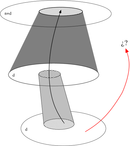
Figure 1: Pictorial representation of an entire truncation scheme. From top to bottom: the initial truncation corresponds to a dimensional reduction, $d+n\rightarrow d$, with ${\mathcal{L}}\rightarrow{\mathcal{L}}_{R}$. The upper shadowed area indicates the solutions of the original theory that fulfil the Killing conditions. The second-type truncation is performed in a second step, ${\mathcal{L}}_{R}\rightarrow{\mathcal{L}}_{2R}$. It concerns only with a reduction of the degrees of freedom in the theory, thus the dimensionality of the space-time is maintained. The total intermediate region describes the solutions of the ${\mathcal{L}}_{R}$ theory, whereas the shadowed area inside corresponds to the solutions that in addition satisfy some given primary constraints (in our example, the constraints (4.3)). The lower region describes the solutions of the ${\mathcal{L}}_{2R}$ theory and the shadowed area in it describes those that can be uplifted to solutions of the ${\mathcal{L}}_{R}$ theory because they satisfy the secondary constraints (in our example, the constraints (5.10)).

6 Conclusions

In this paper we have clarified the issue of consistent truncations, giving them a proper definition and classifying them into two types: a first-type, corresponding to a Kaluza-Klein dimensional reduction that keeps unchanged the number of degrees of freedom attached to every space-time point, and a second-type, where configuration-space constraints are introduced that reduce the number of degrees of freedom per space-time point. As a byproduct we link in a natural way the issue of consistent truncations of theories with that of correct uplifting of solutions.

As regards the first-type, we prove the tracelessness condition for a consistent truncation under a Lie algebra of independent Killing vector fields. Our proof is at the level of the Euler-Lagrange equations of motion, and is complementary to the results in [11] and in [12]. We emphasise that the proof is complete as regards the aspects of necessity and sufficiency of the tracelessness condition. Establishing the conditions for a consistent truncation under Lie algebras whose generators are not independent remains an open problem and, up to now, it seems that there is no group-theoretical argument that can anticipate whether a given reduction will eventually be a consistent one.

We also discuss the full reduction of the gauge group in the common cases of the Maxwell $U(1)$ gauge group and the space-time diffeomorphisms group. The reduction is worked out in full detail and it is shown in particular that a residual rigid group of symmetries, associated with the outer automorphisms of the Lie algebra, remains in the formalism.

With regard to second-type truncations we show that there is a useful link with the Dirac-Bergmann theory of constrained systems, which we find worth to exploit. In particular we explicitate with an example the fact that the these truncations will usually be inconsistent due to the presence of secondary constraints, which are dynamically derived from the primary ones used to define the truncation. In spite of these obstructions to a consistent truncation, we show how one can still have correct upliftings if it happens that there exists a subset of solutions of the truncated theory that satisfy the secondary constraints.

Our results indeed reinforce the definition of consistent truncation we make use throughout the paper, reflected in the diagram of the introductory section.

Acknowledgements J. M. P. thanks the theoretical physics group at the Imperial College London for the warm hospitality during the early stages of this work. This work is partially supported by MCYT FPA, 2001-3598, CIRIT, GC 2001SGR-00065, and HPRN-CT-2000-00131.

Appendix A Lagrangian $y$-dependences

Proposition: All the $y$-dependences in the Lagrangian are encoded in the single factor $|\omega|$ in (2.19).

Proof. Since the Lagrangian is a scalar density and all the fields present in it satisfy the Killing conditions (which is the point of departure for the reduction procedure), so it does the Lagrangian itself,

$${\mathfrak{L}}_{{\bf K}_{a}}{\mathcal{L}}=\partial_{\alpha}({\mathcal{L}}\,K_{a}^{\alpha})=0\,.$$

On the other hand, the commutation relations (2.3) imply

$$\partial_{\alpha}(K_{a}^{\alpha})=|\omega|{\bf K}_{a}\left(\frac{1}{|\omega|}\right)\,.$$ (A.1)

Then,

$$\partial_{\alpha}\,({\mathcal{L}}\,K_{a}^{\alpha})={\bf K}_{a}{\mathcal{L}}+{\mathcal{L}}|\omega|{\bf K}_{a}\left(\frac{1}{|\omega|}\right)={|\omega|}{\bf K}_{a}\left(\frac{{\mathcal{L}}}{|\omega|}\right)\,,$$ (A.2)

together with the condition ${\mathfrak{L}}_{{\bf K}_{a}}{\mathcal{L}}=0$ amounts to ${\bf K}_{a}\left(\frac{{\mathcal{L}}}{|\omega|}\right)=0$ or, equivalently to, $\partial_{\alpha}\left(\frac{{\mathcal{L}}}{|\omega|}\right)=0$, which means that ${\mathcal{L}}$ is of the form

$${\mathcal{L}}(x,y)=|\omega|f(x)\,,$$ (A.3)

for some scalar function $f$ that depends exclusively of the $x$-coordinates.  

Appendix B Scalars associated with p-forms and bi-invariance

In this appendix, we shall see that, for semi-simple Lie algebras, the constraints imposed by the bi-invariance requirement on any $p$-form, set the components that become scalars under the reduction process identically to zero.

• In the one-forms case the constraint (4.6) gives

  $$0=\Omega_{a}C^{a}_{cd}=\Omega^{e}h_{ea}C^{a}_{cd}=\Omega^{e}h_{da}C^{a}_{ce}\,\Rightarrow\,\Omega^{e}C^{a}_{ce}=0\,\Rightarrow\,\Omega^{e}h_{ef}=0\,\Rightarrow\,\Omega^{e}=0$$

  which implies

  $$\Omega_{a}=0\,.$$ (B.1)

• When two-forms (2.16) are present, the constraint (4.7) imposes

  $$0=\Omega_{ba}C^{a}_{cd}-\Omega_{da}C^{a}_{cb}=\Omega_{b}^{\ e}h_{ea}C^{a}_{cd}-\Omega_{d}^{\ e}h_{ea}C^{a}_{cb}=\Omega_{b}^{\ e}h_{da}C^{a}_{ce}-\Omega_{d}^{\ e}h_{ba}C^{a}_{ce}\,,$$

  where $h_{ab}$ satisfies (4.9). The previous expression implies, saturating with $h^{bf}h^{dg}$,

  $$\Omega^{fe}C^{g}_{ce}-\Omega^{ge}C^{f}_{ce}=0\,.$$ (B.2)

  Saturating (B.2) with $C^{c}_{gd}$, one obtains

  $$\Omega^{f}_{\ d}=\Omega^{ge}C^{f}_{ce}C^{c}_{gd}=\Omega^{ge}(C^{f}_{cg}C^{c}_{ed}+C^{f}_{cd}C^{c}_{ge})\,.$$

  A direct consequence of (B.2) is obtained using the tracelessness condition $C^{f}_{fe}=0$

  $$\Omega^{fe}C^{g}_{fe}=0\,.$$ (B.3)

  Using (B.3), the antisymmetry property of $\Omega^{ge}$ and the Jacobi identity we obtain

  $$\Omega^{f}_{\ d}=\Omega^{ge}C^{f}_{cg}C^{c}_{ed}=\frac{1}{2}\Omega^{ge}(C^{f}_{cg}C^{c}_{ed}-C^{f}_{ce}C^{c}_{gd})=\frac{1}{2}\Omega^{ge}C^{f}_{cd}C^{c}_{ge}=0\,.$$

  Concluding that

  $$\Omega_{ab}=0.$$ (B.4)

The proof of the vanishing of the scalars coming from p-forms can be generalised to $p>2$. Summing up, our constraints imply –when the Lie algebra is semi-simple– that the scalars produced from the forms must vanish.

References

- [1] M. J. Duff, B. E. Nilsson, C. N. Pope and N. P. Warner, Phys. Lett. B 149 (1984) 90.
- [2] M. J. Duff and C. N. Pope, Nucl. Phys. B 255 (1985) 355.
- [3] M. J. Duff, B. E. Nilsson, N. P. Warner and C. N. Pope, Phys. Lett. B 171 (1986) 170.
- [4] M. J. Duff, S. Ferrara, C. N. Pope and K. S. Stelle, Nucl. Phys. B 333 (1990) 783.
- [5] Th. Kaluza, Sitzungsber. Preuss. Akad. Wiss. Berlin, Math. Phys. K1 (1921) 996.
- [6] O. Klein, Z.F.Phyzik 37 (1926) 895; Nature 118 (1926) 516.
- [7] M. J. Duff, B. E. Nilsson and C. N. Pope, “Kaluza-Klein Supergravity,” Phys. Rept. 130 (1986) 1.
- [8] T. Appelquist, A. Chodos and P. G. Freund, “Modern Kaluza-Klein Theories,” Reading, USA: Addison-Wesley (1987) 619 P. (Frontiers in Physics, 65).
- [9] S. W. Hawking, “On the rotation of the universe,” Mon. Not. R. Astron. Soc. 142 (1969) 129.
- [10] G. E. Sneddon, “Hamiltonian cosmology: a further investigation,” J. Phys. Math. Gen. 9 (1976) 229.
- [11] J. Scherk and J. H. Schwarz, “How To Get Masses From Extra Dimensions,” Nucl. Phys. B 153 (1979) 61.
- [12] M. A. MacCallum, “Anisotropic And Inhomogeneous Relativistic Cosmologies,” In Hawking, S.W., Israel, W.: General Relativity, an Einstein centenary survey. Cambridge University Press, 1979, pags 533-580.
- [13] J. M. Pons and L. C. Shepley, “Dimensional reduction and gauge group reduction in Bianchi-type cosmology,” Phys. Rev. D 58 (1998) 024001 [arXiv:gr-qc/9805030].
- [14] A. Krasinski, C. G. Behr, E. Sch cking, F. B. Estabrook, H. D. Wahlquist, G. F. R. Ellis, R. Jantzen, W. Kundtpp. “The Bianchi Classification in the Sch cking-Behr Approach,” Gen. Rel. Grav. 35 (2003) 475-489.
- [15] M. Cvetic, G. W. Gibbons, H. Lu and C. N. Pope, “Consistent group and coset reductions of the bosonic string,” arXiv:hep-th/0306043.
- [16] L. O’Raifeartaigh, “Group Structure Of Gauge Theories,” Cambridge, Uk: Univ. Pr. ( 1986) 172 P. ( Cambridge Monographs On Mathematical Physics).
- [17] A. Ashtekar and J. Samuel, “Bianchi Cosmologies: The Role Of Spatial Topology,” Class. Quantum Grav. 8 (1991) 2191.
- [18] B. S. De Witt, In C. and B. S. De Witt (ed.) “Relativity, Groups And Topology”, Gordan and Breach, New York (1964).
- [19] L. O’Raifeartaigh, “The Dawning Of Gauge Theory,” Princeton, USA: Univ. Pr. (1997) 249 p.
- [20] J. M. Pons, “Plugging The Gauge Fixing Into The Lagrangian,” Int. J. Mod. Phys. A 11 (1996) 975 [arXiv:hep-th/9510044].
- [21] Y. M. Cho and P. G. Freund, “Nonabelian Gauge Fields In Nambu-Goldstone Fields,” Phys. Rev. D 12 (1975) 1711.
- [22] A. Jadczyk, “Symmetry Of Einstein Yang-Mills Systems And Dimensional Reduction,” J. Geom. Phys. 1 ( 1984) 97.
- [23] P. A. Dirac, “Generalized Hamiltonian Dynamics,” Can. J. Math. 2 (1950) 129.
- [24] P. A. M. Dirac, “Lectures on Quantum Mechanics,” (Yeshiva Univ. Press, New York, 1964)
- [25] P. G. Bergmann, “Non-Linear Field Theories,” Phys. Rev. 75 (1948) 680.
- [26] P. G. Bergmann and J. H. M. Brunings, “ Non-Linear Field Theories II. Canonical Equations and Quantization,” Rev. Mod. Phys. 21 (1949) 480.
- [27] J. L. Anderson and P. G. Bergmann, “Constraints In Covariant Field Theories,” Phys. Rev. 83 (1951) 1018.