Maximal Locality and Predictive Power in Higher-Dimensional, Compactified Field Theories

Abstract

To achieve a maximal locality in a trivial field theory, we maximize the ultraviolet cutoff of the theory by fine tuning the infrared values of the parameters. This optimization procedure is applied to the scalar theory in $D+1$ dimensions ($D\geq 4$) with one extra dimension compactified on a circle with radius $R$. The optimized, infrared values of the parameters are then compared with the corresponding ones of the uncompactified theory in $D$ dimensions, which is assumed to be the low-energy effective theory. We find that these values approximately agree with each other, as long as $R^{-1}\mathrel{\mathchoice{\vbox{\offinterlineskip\halign{$\m@th\displaystyle\hfil#\hfil$\cr>\crcr\sim\crcr} }}{\vbox{\offinterlineskip\halign{$\m@th\textstyle\hfil#\hfil$\cr>\crcr\sim\crcr} }}{\vbox{\offinterlineskip\halign{$\m@th\scriptstyle\hfil#\hfil$\cr>\crcr\sim\crcr} }}{\vbox{\offinterlineskip\halign{$\m@th\scriptscriptstyle\hfil#\hfil$\cr>\crcr\sim\crcr} }}}sM$ is satisfied, where $s\simeq 10,50,50,100$ for $D=4,5,6,7$, and $M$ is a typical scale of the $D$-dimensional theory. This result supports the previously made claim that the maximization of the ultraviolet cutoff in an nonrenormalizable field theory can give the theory more predictive power.

1 Introduction

Since Kaluza and Klein [1] found a possibility of unifying fundamental forces by introducing extra dimensions, their idea has attracted attentions for many decades. Recently, there have been renewed interests in field theories with extra dimensions. [2]dienes1 Since field theories in more than four dimensions are usually nonrenormalizable, the dependence of the UV cutoff can not be completely removed, and moreover one has to introduce infinitely many independent parameters in these theories. In short, nonrenormalizable theories have much less predictive power compared with renormalizable theories. In our previous paper [7], we proposed a method, called maximal locality method, to make nonrenormalizable theories more predictive. The method is based on a simple intuitive picture that the renormalization group (RG) flow of the effective theory of a fundamental theory, which evolves for “maximal running time”, will be the best approximation to the renormalized trajectory of the fundamental theory.

In this work, we apply the method to compactified higher dimensional theories, and will consider in particular the scalar theory in $D+1$ dimensions with one dimension compactified on a circle with radius $R$. One intuitively expects that the $D$ dimensional theory with all the Kaluza-Klein massive modes suppressed is the low-energy effective theory of the original $(D+1)$-dimensional theory. So, the predictions of the $D$ dimensional effective theory and the original $(D+1)$-dimensional theory should agree with each other at low energies. Therefore, if maximal locality method is a sensible method, it has to satisfy this consistency. We find that there exits a maximal radius above which the consistency requirement can not be satisfied.

This paper is organized as follows. In Sect. 2, we outline of the basic idea of maximal locality method with a concrete example. In Sect. 3 we derive a RG equation in the local potential approximation (the Wegner-Houghton equation) for compactified scalar theories. The five-, six-, seven-, and eight-dimensional scalar theories are considered in Sect. 4, and we estimate the maximal radius for each case. Lastly we conclude in Sect. 5, and the explicit expressions for the $\beta$-functions which we use in this paper are given in AppendixA.

2 Maximal Locality Method

2.1 Formulation

The basic idea of maximal locality method is based on a simple intuitive picture. Consider a theory, like QCD, which is free from the UV cutoff, $\Lambda_{0}$, and suppose its low-energy effective theory, like non-linear sigma model, is a perturbatively nonrenormalizable, trivial theory that becomes weakly coupling in the infrared (IR) regime. We then formulate both theories in terms of the Wilsonian renormalization group (RG) [8]. Since we assume that the high-energy theory is free from the UV cutoff, $\Lambda_{0}$, we can let go $\Lambda_{0}$ to infinity. In other words, the RG flow in the high-energy theory evolves along a renormalized trajectory, and approaches an UV fixed point in the UV limit. The flow has to evolve for “infinite time” to arrive at the fixed point [8]. At low energies, the RG flow obtained in the effective theory should be a good approximation to the corresponding one of the high-energy theory. However, within the frame work of the effective theory, the UV cutoff $\Lambda_{0}$ can not become infinite, or the RG flow does not converge to a fixed point. Above some scale $\Lambda_{\rm H}$, the effective theory is no longer effective, and should be replaced by the high-energy theory to obtain the correct high-energy behavior of the RG flow.

So far there is nothing special. Suppose now we have a trivial theory that well describes low energy physics, but we do not know about its high-energy theory. Our basic assumption is that the RG flow in the effective theory that evolves for “maximal time” may be the best approximation to the renormalized trajectory of the unknown high-energy theory. This optimized RG flow can be obtained by fine tuning the IR values of the dependent parameters of the effective theory. If the theory is perturbatively renormalizable, we regard the coupling constants with a negative canonical dimension as dependent parameters. In the case of perturbatively nonrenormalizable theory, we regard the coupling constants with a canonical dimension $d\geq d_{\rm max}<0$ as independent parameters, while we regard the coupling constants with $d<d_{\rm max}$ as dependent parameters. (The value of the maximal canonical dimension $d_{\rm max}$ depends on the theory, and we do not know it a priori.) Then we require that, for given low-energy values of the independent parameters, the low-energy values of the dependent parameters are so fine tuned as to reach the maximal UV cutoff $\Lambda_{\rm max}$. The effective theory so optimized will behave as a local field theory to the shortest distance ($\sim\Lambda^{-1}_{\rm max}$). This is why we would like to call this optimizing method maximal locality method. In [7] we considered the uncompactified scalar theories in higher dimensions, and found that the maximization of the UV cutoff in an nonrenormalizable field theory can give the theory more predictive power, at least in lower orders of the local potential approximation to the exact RG equation.

2.2 Continuous Wilsonian Renormalization Group

As we have mentioned above, our interest is directed to trivial theories. To define such theories in a non-perturbative fashion, we have to introduce a cutoff. A natural framework to study cutoff theories is provided by the continuous Wilsonian RG [8]. Let us briefly illustrate the basic idea of the Wilsonian RG approach in the case of $N$ components scalar theory in flat Euclidean $D$ dimensions. As first, we divides the field $\phi(p)$ in the momentum space into lower and higher energy modes than the cutoff $\Lambda$ according to

$$\phi^{a}(p)=\theta(|p|-\Lambda)~{}\phi^{a}_{>}(p)+\theta(\Lambda-|p|)\phi^{a}_{<}(p),~{}~{}a=1,\cdots,N.$$ (1)

Then the Wilsonian effective action at $\Lambda$ is defined by integrating out only the higher energy modes $\phi^{a}_{>}$ in the path integral,

$$S_{\rm eff}[\phi_{<},\Lambda]=-\ln\left\{\int{\cal D}\phi_{>}e^{-S[\phi_{>},\phi_{<}]}\right\}.$$ (2)

It was shown that the path integral corresponding to the difference between $\Lambda$ and $\Lambda+\delta\Lambda$

$$\delta S_{\rm eff}=S_{\rm eff}[~{}\phi_{<},\Lambda+\delta\Lambda~{}]-S_{\rm eff}[~{}\phi_{<},\Lambda~{}]$$ (3)

for an infinitesimal $\delta\Lambda$ can be exactly carried out. This yields the non-perturbative (exact) renormalization group evolution equation for the effective action

$$\frac{\partial S_{\rm eff}}{\partial t}=-\Lambda\frac{\partial S_{\rm eff}}{\partial\Lambda}={\cal O}(S_{\rm eff}),$$ (4)

where ${\cal O}$ is a non-linear operator acting on the functional $S_{\rm eff}$. There exist various (equivalent) formulations of regularizations, but in this paper we consider only the Wegner-Houghton equation [9]. Since $S_{\rm eff}$ is a functional of fields, one can think of the Wegner-Houghton equation as coupled differential equations for infinitely many couplings in the effective action. The crucial point is that ${\cal O}$ can be exactly derived for a given theory, in contrast to the perturbative renormalization group approach where the RG equations are known only up to a certain order in perturbation theory. This provides us with possibilities to use approximation methods that go beyond the conventional perturbation theory. Therefore Wilsonian RG approach is suitable for maximal locality method which deals with non-perturbative effects of nonrenormalizable theory.

2.3 Example: Uncompactified Four-Dimensional Scalar Theory

In this subsection we would like to illustrate how maximal locality method works even in a perturbatively renormalizable, but trivial theory. We shall consider an uncompactified four-dimensional scalar theory with four components. The theory is perturbatively renormalizable, but presumably it is trivial [20, 12, 21]. Here we assume that it is trivial. Perturbative series are only asymptotic series, and suffer from a non-perturbative ambiguity which originates from the renormalon singularity in the Borel plane [10]. We will see that the method can remove this ambiguities.

At first, in the derivative expansion approximation, [16, 13] [17]aoki1 one assumes that the effective action $S_{\rm eff}[\phi,\Lambda]$ can be written as a space-time integral of a (quasi) local function of $\phi$, i.e.,

$$S_{\rm eff}[\phi,\Lambda] = \int d^{D}x\left(\frac{1}{2}\,\sum_{k,l=1}^{N}\partial_{\mu}\phi^{k}\partial_{\mu}\phi^{l}Z^{kl}(\phi,\Lambda)+V(\phi,\Lambda)+\cdots\right),$$ (5)

where $\cdots$ stands for terms with higher order derivatives with respect to the space-time coordinates, and $N$ is a number of scalar components. In the lowest order of the derivative expansion (the local potential approximation), there is no wave function renormalization, i.e. $Z^{kl}(\phi,\Lambda)=\delta^{kl}$, and the RG equation for the effective potential $V$ can be obtained. Since it is more convenient to work with the RG equation for dimensionless quantities, which makes the scaling properties more transparent, we rescale the quantities according to

$$p\to\Lambda p,~{}~{}\phi_{a}\to\Lambda^{\frac{D}{2}-1}\phi_{a},~{}~{}V\to\Lambda^{D}V.$$ (6)

Then the RG equation for $V(\phi,\Lambda)$ is given by [13]

$$\frac{\partial V}{\partial t} = -\Lambda\frac{\partial V}{\partial\Lambda}$$ (7)

$$= DV+(2-D)\rho V+\frac{A_{D}}{2}\Bigl{[}(N-1)\ln(1+V^{\prime})+\ln(1+V^{\prime}+2\rho V^{\prime\prime})\Bigr{]}$$

where the prime on $V$ stands for the derivative with respect to $\rho$, and

$$\rho=\frac{1}{2}\sum_{a=1}^{N}\phi_{a}\phi_{a}~{},~{}~{}A_{D}=\frac{1}{2^{D-1}\pi^{D/2}\Gamma(D/2)}.$$ (8)

In the case of $D=4$, we have $A_{4}=1/8\pi^{2}$. Eq. (7) is the Wegner-Houghton equation for the effective potential of the $D$-dimensional $O(N)$ scalar theory. The equation (7) is equivalent to the following equation for $F\equiv\partial V/\partial\rho$,

$$\frac{\partial F}{\partial t}=2F+(2-D)\rho F^{\prime}+\frac{A_{D}}{2}\left[(N-1)\frac{F^{\prime}}{1+F}+\frac{3F^{\prime}+2\rho F^{\prime\prime}}{1+F+2\rho F^{\prime}}\right].$$ (9)

To solve eq. (9) in the local potential approximation, we expand the effective potential $V$ as

$$V(\rho,t) = v_{0}(t)+\sum_{n=1}^{\infty}\frac{1}{n+1}\frac{f_{n}(t)}{{(2A_{D})}^{n}}\Bigl{[}\rho-2A_{D}f_{0}(t)\Bigr{]}^{n+1}$$ (10)

$$= v_{0}(t)+\frac{1}{2}\frac{f_{1}(t)}{2A_{D}}{\Bigl{[}\rho-2A_{D}f_{0}(0)\Bigr{]}}^{2}+\frac{1}{3}\frac{f_{2}(t)}{(2A_{D})^{2}}{\Bigl{[}\rho-2A_{D}f_{0}(0)\Bigr{]}}^{3}+\cdots.$$

$F$ can also be expanded, and by inserting expanded form of $F$ into eq. (9), we can obtain a set of $\beta$ functions, $\beta_{n}=df_{n}/dt$, at any finite order of truncation.

Next to see the relation between perturbative renormalizability and the nonperturbative ambiguity, we solve the reduction equation, [22]

$$\beta_{1}\frac{df_{n}}{df_{1}} = \beta_{n}~{},~{}(n\neq 1)~{},$$ (11)

near the Gaussian fixed point $(f_{0}=3/4~{},~{}f_{n}=0~{}(n\geq 1))$ for $D=4$ and $N=4$. We find that the general solution for $(n\leq 2)$, for instance, takes the form

$$f_{0} = \frac{3}{4}-\frac{9}{16}f_{1}^{2}+\frac{225}{64}f_{1}^{2}-\frac{7857}{256}f_{1}^{3}+\frac{269001}{1024}f_{1}^{4}-\frac{12806991}{4096}f_{1}^{5}+\frac{650870883}{16384}f_{1}^{6}+O(f_{1}^{7})$$ (12)

$$+K_{2}\exp\left(-\frac{2}{3f_{1}}-\frac{57}{4}f_{1}\right)~{}f_{1}^{7/2}~{}\left[\frac{3}{16}-\frac{9}{8}f_{1}+\frac{2799}{256}f_{1}^{2}+O(f_{1}^{3})~{}\right]~{},$$

$$f_{2} = \frac{15}{4}f_{1}^{3}-\frac{189}{8}f_{1}^{4}+\frac{7479}{64}f_{1}^{5}-\frac{12879}{32}f_{1}^{6}+O(f_{1}^{7})+K_{2}\exp\left(-\frac{2}{3f_{1}}-\frac{57}{4}f_{1}\right)~{}f_{1}^{9/2}~{},$$

where $K_{2}$ is an integration constant. We see from the above solution that the exponential function $\exp{(-2/3f_{1})}$ decreases fast as $f_{1}$ approaches zero, so that the ambiguity involved in the integration constant $K_{2}$ becomes negligible in the infrared limit. In this limit, the power series part of the above solution (LABEL:generaln) becomes dominant. In other words, the power series solution is infrared attractive. This infrared attractiveness is interpreted as perturbative renormalizability by Polchinski [11].

As we will argue below, the exponential part of (LABEL:generaln) is a non-perturbative ambiguity [12]. We have computed higher orders in the power series expansion (LABEL:generaln) and found that they do not approximate the exact (numerical) result better. The one with the first four terms in (LABEL:generaln) is the best approximation among lower orders. From this fact, we believe that the power series solution (LABEL:generaln) does not converge, and that it is an asymptotic series. So, this power series reflects the property of perturbation series in the conventional perturbation theory, as far as our numerical analysis in lower orders suggests. This interpretation is also supported by the fact that not only the leading form of the nonperturbative ambiguity, the last exponential term in (LABEL:generaln), agrees with that of the known renormalon ambiguity [10], but also the coefficient of $1/f_{1}$, $2/3$, in the exponential function. The power of $f_{1}$ in front of the exponential function, that is $9/2$, differs slightly from the expected value $3$. The origin is presumably the local potential approximation to the exact RG evolution equation. We believe that the last term in (LABEL:generaln) is the renormalon ambiguity.

According to the formulation of our method in Sect. 2.1, we should regard $f_{0}$ and $f_{1}$ as independent parameters, while the other coupling constants $f_{n}(n\geq 2)$ as dependent parameters. Then, using a set of $\beta$ functions for each coupling constants, we investigate the running time $T_{0}=\ln(\Lambda_{0}/\Lambda)$ against $f_{n}(t=0)\ (n\geq 2)$ for given $f_{0}(0)$ and $f_{1}(0)$.

Figure 1: Fine-tuning of $f_{2}(0)$ for given values $(f_{0}(0),~{}f_{1}(0))=(1/2A_{4},~{}0.10)$ in uncompactified four-dimensional case for the truncation at $n=2$. The running time $T_{0}=\ln(\Lambda_{0}/\Lambda)$ is peaked at $f_{2}(0)\simeq 0.000528$.

Figure 2: Fine-tuning of $f_{2}(0)$ and $f_{3}(0)$ for $(f_{0}(0),~{}f_{1}(0))=(1/2A_{4},~{}0.79)$ in the case of truncation at $n=3$. $T_{0}$ is peaked at $(f_{2}(0),~{}f_{3}(0))\simeq(0.19285,~{}0.0112)$ .

Fig. 1 and Fig. 2 show the results for given values, $(f_{0}(0),~{}f_{1}(0))=(1/2A_{4},~{}0.10)$, in the case of the truncation level at $n=2$, and for given $(f_{0}(0),~{}f_{1}(0))=(1/2A_{4},~{}0.79)$ at $n=3$ respectively. From these figures, we can see that $T_{0}$ is peaked at $f_{2}(0)\simeq 0.000528$ for $n=2$, and peaked at $(f_{2}(0),~{}f_{3}(0))\simeq(0.19285,~{}0.0112)$ for $n=3$. Then maximal locality method requires that the dependent coupling constants $f_{n}~{}(n\geq 2)$ must be so fine tuned that $T_{0}$ becomes maximal. In this way we can determine the values of the dependent parameters for a given finite number of the independent parameters.

Figure 3: Determination of the nonperturbative coefficient $K_{2}$ (given in (LABEL:generaln)) in $D=4$.

This implies that the constant $K_{2}$ in (LABEL:generaln), which exhibits a nonperturbative correction of the renormalon type [10, 12], is also fixed. In Fig. 3 we plot $T_{0}$ against $K_{2}$. From this result we obtain

$$K_{2} \simeq 7\times 10^{3}~{}.$$ (14)

This means a departure of about $3~{}(0.1)$ % from the perturbative result at $f_{1}=0.1~{}(0.07)$. Needless to say that the corresponding effect in the standard model could be in principle measurable.

3 Application to the Compactified Theories

3.1 The Action

We now come to consider the Kaluza-Klein theory for the $N$ components scalar field in Euclidean $D+1$ dimensions where we assume that the one dimension is compactified on a circle with radius $R$. We denote the one compactified coordinate by $y$ and other flat coordinates by $x_{M}$ $(M=0,1,\cdots,D)$.

We start with the following action in $(D+1)$-dimensions:

$$S_{D+1}=\int d^{D}x\int^{2\pi R}_{0}dy\left\{\frac{1}{2}\sum_{a}^{N}\left({(\partial_{M}\Phi_{a})}^{2}+{(\partial_{y}\Phi_{a})}^{2}\right)+V_{D+1}(\Phi_{b})\right\},$$ (15)

where $V_{D+1}$ is the $(D+1)$-dimensional potential. As eq. (10), $V$ is assumed to be expanded as

$$V_{D+1}=v_{0}(t)+\sum_{m=1}^{\infty}\frac{f_{m}(t)}{(2A_{D+1})^{m}}\left[\frac{1}{2}\sum_{a}\Phi_{a}\Phi_{a}-2A_{D+1}f_{0}(t)\right]^{m+1}.$$ (16)

The scalar field $\Phi$ satisfies the boundary condition on the extra coordinate $y$,

$$\Phi_{a}(x,y)=\Phi_{a}(x,y+2\pi R)\ .$$ (17)

Then the field can be expanded as

$$\Phi_{a}(x,y)=\sum_{n\in{\bf Z}}e^{in\frac{y}{R}}\phi^{(n)}_{a}(x)~{}.$$ (18)

$\phi^{(n)}$ is $n$-th Kaluza-Klein mode. After we appropriately perform rescaling to the field and coupling constants, and integrate out only $y$ coordinate of extra dimension, we obtain the $D$-dimensional potential

$$V_{D} = {v_{0}}^{\prime}(t)+\frac{1}{2}\left(f_{0}^{2}f_{2}-f_{0}f_{1}\right)\sum_{a}\sum_{n}\phi_{a}^{(n)}\phi_{a}^{(-n)}$$ (19)

$$+\frac{1}{8A_{D}}\left(\frac{1}{2}f_{1}-f_{0}f_{2}\right)\sum_{a,b}\sum_{n_{i}}\phi_{a}^{(n_{1})}\phi_{a}^{(n_{2})}\phi_{b}^{(n_{3})}\phi_{b}^{(n_{4})}~{}\delta_{n_{1}+n_{2}+n_{3}+n_{4},~{}0}$$

$$+\frac{1}{24(2A_{D})^{2}}f_{2}\sum_{a,b,c}\sum_{n_{i}}\phi_{a}^{(n_{1})}\phi_{a}^{(n_{2})}\phi_{b}^{(n_{3})}\phi_{b}^{(n_{4})}\phi_{c}^{(n_{5})}\phi_{c}^{(n_{6})}~{}\delta_{n_{1}+n_{2}+n_{3}+n_{4}+n_{5}+n_{6},~{}0}$$

$$+\cdots,$$

and the action in $D$-dimensions

$$S_{D}=\int d^{D}x\left\{\frac{1}{2}\sum_{a=1}^{N}\sum_{n\in{\bf Z}}\phi^{(-n)}_{a}\left(-\partial_{M}^{2}+m_{n}^{2}\right)\phi^{(n)}_{a}+V_{D}(\phi^{(l)}_{b})\right\},$$ (20)

where $m_{n}$ is $n$-th mode Kaluza-Klein masses,

$$m_{n}=\frac{n}{R}\ .$$ (21)

As we have seen, the compactified $(D+1)$-dimensional theory yields an infinite number of Kaluza-Klein modes at the viewpoint of the flat $D$-dimensional theory.

3.2 Wegner-Houghton Equation for Compactified Scalar Theories

Now we would like to investigate the Wegner-Houghton equation for the compactified $(D+1)$-dimensional scalar theory in the $D$-dimensional sense. In the lowest order of derivative expansion approximation, we assume the following effective action for the compactified theory

$$S_{\rm eff}[\phi^{(l)}_{b},t]=\int d^{D}x\left\{\frac{1}{2}\sum_{a=1}^{N}\sum_{n\in{\bf Z}}\phi^{(-n)}_{a}\left(-\partial_{M}^{2}+m_{n}^{2}\right)\phi^{(n)}_{a}+V_{\rm eff}(\phi^{(l)}_{b},t)\right\}.$$ (22)

Then the RG equation for the effective potential $V_{\rm eff}$ can be obtained. As in Sect. 2.3, we rescale the quantities according to eq. (6) and

$$m_{n}\to\Lambda m_{n}.$$ (23)

The RG equation (Wegner-Houghton equation) for the effective potential $V$ is given by

$$\frac{\partial V}{\partial t} = -\Lambda\frac{\partial V}{\partial\Lambda}$$ (24)

$$= DV-\frac{D-2}{2}\sum_{n}\sum_{a}\phi_{a}^{(n)}\frac{\partial V}{\partial\phi_{a}^{(n)}}+\frac{A_{D}}{2}{\rm Tr}\ln\left(1+m_{n}^{2}+\frac{\partial^{2}V}{\partial\phi_{a}^{(n)}\partial\phi_{b}^{(-n)}}\right),$$

where the trace of the second term in the right hand side means summation over the flavor indices $a$ and the Kaluza-Klein mode indices $n$, and $m_{n}$ is rescaled dimensionless Kaluza-Klein masses defined in eq. (23). Note that we have considered only the diagonal parts of the Kaluza-Klein indices in the logarithmic function of the right hand side. Off-diagonal parts in the logarithmic function yield vertices that depend on the external Kaluza-Klein modes, and so this is beyond the local potential approximation, since Kaluza-Klein indices can be regarded as fifth momentum of the field.

Eq. (24) is the central equation that we will analyze in the following. Therefore, all the results we will obtain are valid only within the local potential approximation. From the next section, we would like to investigate the predicted values of the dependent parameters in compactified five-, six-, seven- and eight-dimensional scalar theories, and to check the consistency of the predictions from these theories and the uncompactified flat theories.

4 Results

4.1 Compactified Five-Dimensional Case

We first consider a compactified five-dimensional scalar theory with four components, where one extra dimension is compactified on a circle with radius $R$ and other four dimensions are uncompactified. We would like to find out whether the uncompactified four-dimensional scalar theory can be regarded as the effective theory of the compactified five-dimensional theory, if we apply maximal locality method to the compactified five-dimensional theory as well as to the uncompactified four-dimensional theory. To this end, we make predictions on the dependent parameters at low energy scale $\Lambda_{\rm R}(\ll R^{-1})$ by applying maximal locality method to the compactified theory. We then compare them with those obtained in the uncompactified four-dimensional theory. If it is the low-energy effective theory of the compactified five-dimensional theory, the predicted values should agree with each other.

As in eq. (16), we start with $4+1(=5)$-dimensional potential,

$$V_{4+1(=5)}=v_{0}(t)+\sum_{m=1}^{\infty}\frac{f_{m}(t)}{(2A_{5})^{m}}\left[\frac{1}{2}\sum_{a}\Phi_{a}\Phi_{a}-2A_{5}f_{0}(t)\right]^{m+1},$$ (25)

which defines the coupling constants $f_{m}$. After integrating out only the $y$ coordinate, we appropriately perform rescaling to the field and coupling constants, then we obtain the potential in terms of four-dimensional theory like eq. (19). Then we can obtain a set of $\beta$-functions $\beta_{m}=df_{m}/dt$ from eq. (24) at any finite order truncation. The explicit expressions in lower orders are given in Appendix A. From these explicit expressions, we can see that these $\beta$-functions approach the flat four-dimensional forms as $R\to 0$.

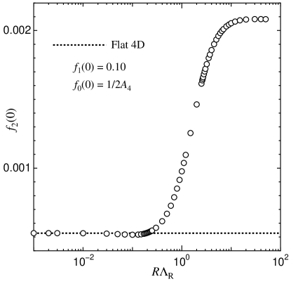
Figure 4: Predicted values of $f_{2}(0)$ for $(f_{0}(0),~{}f_{1}(0))=(1/2A_{4},~{}0.10)$ in compactified five-dimensional theory. The dotted line shows the value in flat four-dimensional theory.

As in the flat four-dimensional case in Sect. 2.1, we have to regard the coupling constants $f_{0}$ and $f_{1}$ as independent parameters, and other coupling constants $f_{m}~{}(m\geq 2)$ as dependent parameters. For the sake of simplicity, we calculate the predicted values of $f_{2}(0)$ at truncation order $m=2$. Fig. 4 shows the predicted values of $f_{2}(0)$ for $(f_{0}(0),~{}f_{1}(0))=(1/2A_{4},~{}0.10)$ as a function of compactification scale $R^{-1}$ varying from $10^{-2}\times\Lambda_{\rm R}$ to $10^{3}\times\Lambda_{\rm R}$, where $\Lambda_{\rm R}$ is renormalization scale (i.e. $t=0$ corresponds to $\Lambda=\Lambda_{\rm R}$). We can see from this figure that the predicted values almost do not differ up to $R\Lambda_{\rm R}\sim 0.1$ from the four-dimensional ones. This means that at most up to $R\Lambda_{\rm R}\sim 0.1$, namely $R^{-1}\mathrel{\mathchoice{\vbox{\offinterlineskip\halign{$\m@th\displaystyle\hfil#\hfil$\cr>\crcr\sim\crcr} }}{\vbox{\offinterlineskip\halign{$\m@th\textstyle\hfil#\hfil$\cr>\crcr\sim\crcr} }}{\vbox{\offinterlineskip\halign{$\m@th\scriptstyle\hfil#\hfil$\cr>\crcr\sim\crcr} }}{\vbox{\offinterlineskip\halign{$\m@th\scriptscriptstyle\hfil#\hfil$\cr>\crcr\sim\crcr} }}}10\times\Lambda_{\rm R}$, the consistency is ensured. This result can also give us the bound for the compactification scale $R^{-1}$. Since the renormalization scale $\Lambda_{\rm R}$ can represent a typical energy scale, it is natural to identify with the Higgs’s VEV. Then we find

$$R^{-1}\mathrel{\mathchoice{\vbox{\offinterlineskip\halign{$\m@th\displaystyle\hfil#\hfil$\cr>\crcr\sim\crcr} }}{\vbox{\offinterlineskip\halign{$\m@th\textstyle\hfil#\hfil$\cr>\crcr\sim\crcr} }}{\vbox{\offinterlineskip\halign{$\m@th\scriptstyle\hfil#\hfil$\cr>\crcr\sim\crcr} }}{\vbox{\offinterlineskip\halign{$\m@th\scriptscriptstyle\hfil#\hfil$\cr>\crcr\sim\crcr} }}}{\rm{\cal O}(TeV)}.$$ (34)

Of course, this bound can change if the value of the independent parameter $f_{1}(0)$ changes. The change will be investigated in Sect. 4.3.

4.2 Compactified Six-, Seven- and Eight-Dimensional Case

Here we consider compactified six-, seven- and eight-dimensional scalar theories. The situation here is different from the previous five-dimensional case, because in the previous case the effective theory was perturbatively renormalizable. In the cases at hand, the compactified as well as lower-dimensional uncompactified theories are nonrenormalizable. We investigate the prediction of the dependent coupling $f_{2}$ at truncation order $m=2$ for various compactification scales.

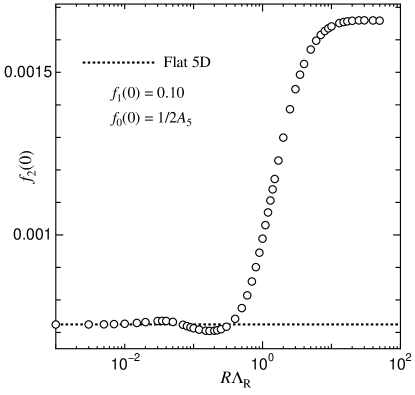
Figure 5: The same as Fig. 4 for $(f_{0}(0),~{}f_{1}(0))=(1/2A_{5},~{}0.10)$ in compactified six-dimensional theory.

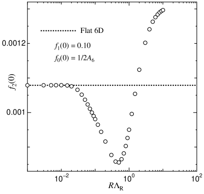
Figure 6: The same as Fig. 4 for $(f_{0}(0),~{}f_{1}(0))=(1/2A_{6},~{}0.10)$ in compactified seven-dimensional theory.

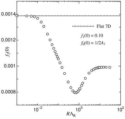
Figure 7: The same as Fig. 4 for $(f_{0}(0),~{}f_{1}(0))=(1/2A_{7},~{}0.10)$ in compactified eight-dimensional theory.

The results are shown in Fig. 5, 6 and 7. To calculate the value $f_{2}(0)$, we have used $(f_{0}(0),~{}f_{1}(0))=(1/2A_{D},~{}0.10)$. From first two figures, we found that

$$R^{-1}\mathrel{\mathchoice{\vbox{\offinterlineskip\halign{$\m@th\displaystyle\hfil#\hfil$\cr>\crcr\sim\crcr} }}{\vbox{\offinterlineskip\halign{$\m@th\textstyle\hfil#\hfil$\cr>\crcr\sim\crcr} }}{\vbox{\offinterlineskip\halign{$\m@th\scriptstyle\hfil#\hfil$\cr>\crcr\sim\crcr} }}{\vbox{\offinterlineskip\halign{$\m@th\scriptscriptstyle\hfil#\hfil$\cr>\crcr\sim\crcr} }}}50\times\Lambda_{\rm R},$$ (43)

is the consistency bound in six and seven dimension cases. This means that if the consistency bound is satisfied, we can predict at low-energies the dependent parameters of the compactified original theory within the framework of the lower-dimensional uncompactified theory by using maximal locality method.

Finally, we show the eight-dimensional case in Fig. 7. We can see from the figure that if compactification scale $R^{-1}$ satisfies the condition

$$R^{-1}\mathrel{\mathchoice{\vbox{\offinterlineskip\halign{$\m@th\displaystyle\hfil#\hfil$\cr>\crcr\sim\crcr} }}{\vbox{\offinterlineskip\halign{$\m@th\textstyle\hfil#\hfil$\cr>\crcr\sim\crcr} }}{\vbox{\offinterlineskip\halign{$\m@th\scriptstyle\hfil#\hfil$\cr>\crcr\sim\crcr} }}{\vbox{\offinterlineskip\halign{$\m@th\scriptscriptstyle\hfil#\hfil$\cr>\crcr\sim\crcr} }}}100\times\Lambda_{\rm R},$$ (52)

the predictions of the compactified and uncompactified theories agree with each other.

4.3 Six-Dimensional Case in Diverse Independent Parameter $f_{1}$

Until to now, we have assume the same value of the independent coupling constant $f_{1}$ at renormalization scale $\Lambda_{\rm R}$, i.e., $f_{1}(0)=0.10$. The prediction of the dependent coupling constants change if the value of $f_{1}(0)$ changes. Here we would like to calculate the change as a function of the independent coupling constant $f_{1}$.

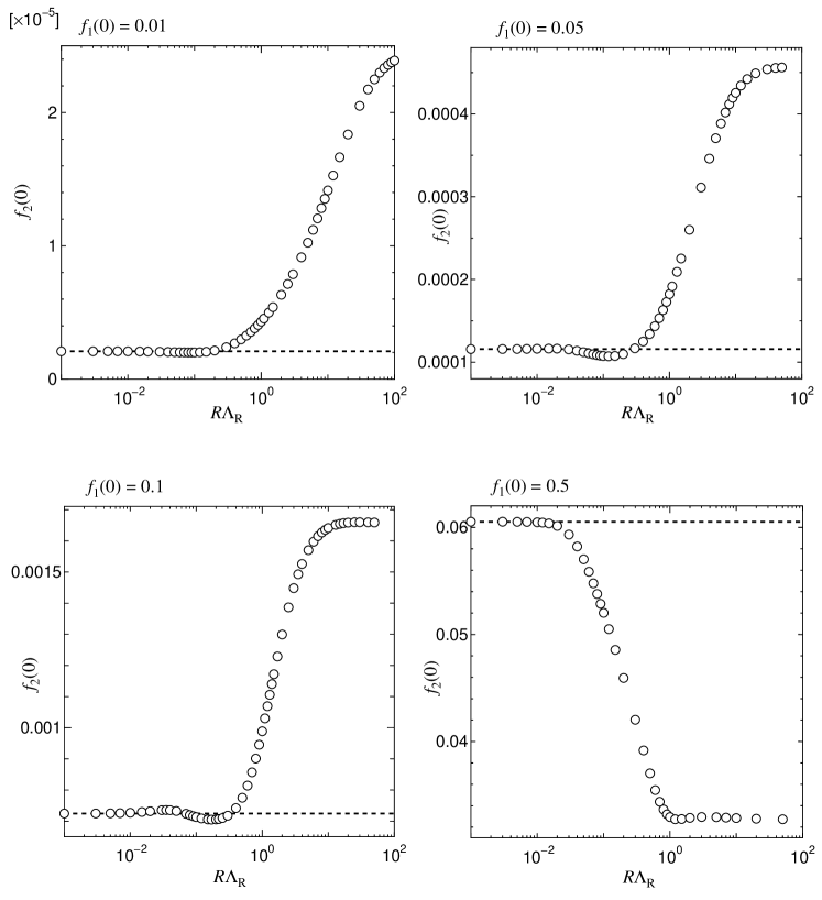
Figure 8: The predictions of $f_{2}(0)$ in the compactified six-dimensional theory for diverse independent parameter $f_{1}(0)$. All figures plot for $f_{0}(0)=1/2A_{5}$, and the dotted line shows the predicted values in the uncompactified five-dimensional theory.

To this end, we consider the compactified six-dimensional scalar theory of the previous subsection, and calculate the consistency bound for the compactification scale as a function of the independent parameter $f_{1}(0)$. In Fig. 8, we show the results for $f_{1}(0)=0.01,~{}0.05,~{}0.10$ and $0.50$ for the same renormalization condition $f_{0}(0)=1/2A_{5}$. As we can see from these figures, the point of $R\Lambda_{\rm R}$ at which the predicted values start to separate from each other, becomes smaller as $f_{1}(0)$ increases. We, therefore, may conclude that as far as $f_{1}(0)\mathrel{\mathchoice{\vbox{\offinterlineskip\halign{$\m@th\displaystyle\hfil#\hfil$\cr<\crcr\sim\crcr} }}{\vbox{\offinterlineskip\halign{$\m@th\textstyle\hfil#\hfil$\cr<\crcr\sim\crcr} }}{\vbox{\offinterlineskip\halign{$\m@th\scriptstyle\hfil#\hfil$\cr<\crcr\sim\crcr} }}{\vbox{\offinterlineskip\halign{$\m@th\scriptscriptstyle\hfil#\hfil$\cr<\crcr\sim\crcr} }}}0.5$, the compactification scale $R^{-1}$ has to satisfy

$$R^{-1}\mathrel{\mathchoice{\vbox{\offinterlineskip\halign{$\m@th\displaystyle\hfil#\hfil$\cr>\crcr\sim\crcr} }}{\vbox{\offinterlineskip\halign{$\m@th\textstyle\hfil#\hfil$\cr>\crcr\sim\crcr} }}{\vbox{\offinterlineskip\halign{$\m@th\scriptstyle\hfil#\hfil$\cr>\crcr\sim\crcr} }}{\vbox{\offinterlineskip\halign{$\m@th\scriptscriptstyle\hfil#\hfil$\cr>\crcr\sim\crcr} }}}50\times\Lambda_{\rm R}$$ (61)

for maximal locality method to consistently work.

5 Conclusion

In particle physics, perturbatively nonrenormalizable theories have played an important role. They are regarded as low-energy effective theories of more fundamental, high-energy theories. Quantum corrections in a nonrenormalizable theory explicitly depends on the UV cutoff, and infinitely many independent parameters can be generated. Nonrenormalizable theories have much less predictive power compared with renormalizable theories, as well known. Field theories in more than four space-time dimensions are usually nonrenormalizable, too. In recent works on extra dimensions, the length scale of extra dimensions is often assumed to be so large that not only the existence of extra dimensions but also quantum corrections could be experimentally observed.

In our previous work [7], we applied the Wilsonian RG to nonrenormalizable theories, and proposed a method to give more predictive power to these theories. The method is based on the assumption on the existence of maximal UV cutoff in a nonrenormalizable theory, and on the requirement that the dependent, low-energy parameters of the theory should be so adjusted that one arrives at a maximal cutoff. A nonrenormalizable cutoff theory, so optimized, behaves as a local field theory as much as possible. In the present work, we considered $(D+1)$-dimensional scalar theories with one extra dimension compactified on a circle. It is naively expected that the uncompactified, flat $D$-dimensional theory is the low-energy effective theory of the compactified $(D+1)$-dimensional theory. We asked ourself, whether or not this expectation is correct, when maximal locality method is employed both in the uncompactified $D$-dimensional and compactified $(D+1)$-dimensional theories. We investigated this question using compactified five-, six-, seven- and eight-dimensional scalar theories with four components. The main finding is that this consistency requirement can strongly constrain the compactification scale $R^{-1}$. We found that for the consistency requirement to be satisfied, the compactification scale $R^{-1}$ should be larger than $\Lambda_{\rm min}=R^{-1}_{\rm max}$, which, depending on the dimension $D$, is $10$ to $100$ times as high as the renormalization scale $\Lambda_{\rm R}$ of the effective theory, a typical energy scale of the low-energy theory. Although this condition for $R$ has been obtained in the derivative expansion approximation in the lowest order to the Wegner-Houghton equation (24), we believe that the gross feature does not depend on the approximation and regularization schemes used.

Finally, we would like to comment on the relation between our method and renormalizability of perturbatively nonrenormalizable theories such as quantum gravity and higher-dimensional Yang-Mills theory. The existence of an UV-fixed point means renormalizability of the theory according to Weinberg.[25] In Ref. QG1, the exact RG equation approaches have been applied to Einstein’s theory of gravity. It has been claimed that within the approximation used in Ref. QG2 there seems to exist an UV-fixed point in the theory. Furthermore, the existence of a continuum limit and an UV-fixed point in Yang-Mills theories in more than four dimensions have been investigated, by lattice Monte-Carlo simulations [28] and by Wilsonian RG approaches [29]. Those results indicate that, even if the UV fixed point does not exist, Einstein’s theory and compactified higher-dimensional Yang-Mills theories can behave as a local field theory to very short distances. Therefore, these theories may have a built-in mechanism to maximize the UV cutoff. We would like to leave the study on this issue to future work.

Appendix A $\beta$-functions for the Compactified Theory

We give here the $\beta$-functions of the coupling constants $f_{m}$ ($m\leq 3$) for $(D+1)$-dimensional four components scalar theory. These functions are described in terms of $D$-dimensional theory, and $R$ is compactification radius.

$$\beta_{0} = (D-2)f_{0}-\frac{3}{4}\pi R\Lambda\coth(\pi R\Lambda)$$

$$-\left(\frac{3}{4}+\frac{f_{0}f_{2}}{f_{1}}\right)\pi R\Lambda\coth{\left(\pi R\Lambda\sqrt{1+2f_{0}f_{1}}\right)}\frac{1}{\sqrt{1+2f_{0}f_{1}}}$$

$$\beta_{1} = (4-D)f_{1}-\frac{3}{4}f_{1}^{2}\left[\frac{1}{2}\pi R\Lambda\left(\coth(\pi R\Lambda)+\pi R\Lambda{\rm\,csch}^{2}(\pi R\Lambda)\right)\right]$$

$$+\left(f_{2}-2\frac{f_{0}f_{2}^{2}}{f_{1}}+3f_{0}f_{3}\right)\pi R\Lambda\coth{\left(\pi R\Lambda\sqrt{1+2f_{0}f_{1}}\right)}\frac{1}{\sqrt{1+2f_{0}f_{1}}}$$

$$-\left(\frac{9}{4}f_{1}^{2}+6f_{0}f_{1}f_{2}+4f_{0}^{2}f_{2}^{2}\right)$$

$$\times\left[\frac{1}{2}\pi R\Lambda\left(\frac{1}{\sqrt{1+2f_{0}f_{1}}}\coth{\left(\pi R\Lambda\sqrt{1+2f_{0}f_{1}}\right)}+\pi R\Lambda{\rm\,csch}^{2}\left(\pi R\Lambda\sqrt{1+2f_{0}f_{1}}\right)\right)\right]\frac{1}{1+2f_{0}f_{1}}$$

$$\beta_{2} = (6-2D)f_{2}-\frac{9}{4}f_{1}f_{2}\left[\frac{1}{2}\pi R\Lambda\left(\coth(\pi R\Lambda)+\pi R\Lambda{\rm\,csch}^{2}(\pi R\Lambda)\right)\right]$$

$$+~{}\frac{3}{4}f_{1}^{3}\left[\frac{3}{8}\pi R\Lambda\left(\coth(\pi R\Lambda)+\pi R\Lambda{\rm\,csch}^{2}(\pi R\Lambda)\right)+\frac{1}{4}{(\pi R\Lambda)}^{3}\coth(\pi R\Lambda){\rm\,csch}^{2}(\pi R\Lambda)\right]$$

$$+\left(3f_{3}-\frac{3f_{0}f_{2}f_{3}}{f_{1}}+6f_{0}f_{4}\right)\pi R\Lambda\coth{\left(\pi R\Lambda\sqrt{1+2f_{0}f_{1}}\right)}\frac{1}{\sqrt{1+2f_{0}f_{1}}}$$

$$-\left(\frac{45}{4}f_{1}f_{2}+15f_{0}f_{2}^{2}+\frac{27}{2}f_{0}f_{1}f_{3}+18f_{0}^{2}f_{2}f_{3}\right)$$

$$\times\left[\frac{1}{2}\pi R\Lambda\left(\frac{1}{\sqrt{1+2f_{0}f_{1}}}\coth{\left(\pi R\Lambda\sqrt{1+2f_{0}f_{1}}\right)}+\pi R\Lambda{\rm\,csch}^{2}\left(\pi R\Lambda\sqrt{1+2f_{0}f_{1}}\right)\right)\right]\frac{1}{1+2f_{0}f_{1}}$$

$$+\left(\frac{27}{4}f_{1}^{3}+27f_{0}f_{1}^{2}f_{2}^{2}+36f_{0}^{2}f_{1}f_{2}^{2}+16f_{0}^{3}f_{2}^{3}\right)$$

$$\times\left[\frac{3}{8}\pi R\Lambda\left(\frac{1}{\sqrt{1+2f_{0}f_{1}}}\coth{\left(\pi R\Lambda\sqrt{1+2f_{0}f_{1}}\right)}+\pi R\Lambda{\rm\,csch}^{2}\left(\pi R\Lambda\sqrt{1+2f_{0}f_{1}}\right)\right)\frac{1}{{(1+2f_{0}f_{1})}^{2}}\right.$$

$$~{}~{}~{}~{}\left.+\frac{1}{4}{(\pi R\Lambda)}^{3}\coth\left(\pi R\Lambda\sqrt{1+2f_{0}f_{1}}\right){\rm\,csch}^{2}\left(\pi R\Lambda\sqrt{1+2f_{0}f_{1}}\right)\frac{1}{{(1+2f_{0}f_{1})}^{\frac{3}{2}}}\right]$$

$$\beta_{3} = (8-3D)f_{3}-\left(3f_{1}f_{3}+\frac{3}{2}f_{2}^{2}\right)\left[\frac{1}{2}\pi R\Lambda\left(\coth(\pi R\Lambda)+\pi R\Lambda{\rm\,csch}^{2}(\pi R\Lambda)\right)\right]$$

$$-~{}\frac{3}{4}f_{1}^{4}\left[\frac{5}{16}\pi R\Lambda\left(\coth(\pi R\Lambda)+\pi R\Lambda{\rm\,csch}^{2}(\pi R\Lambda)\right)+\frac{1}{4}{(\pi R\Lambda)}^{3}\coth(\pi R\Lambda){\rm\,csch}^{2}(\pi R\Lambda)\right.$$

$$~{}~{}~{}~{}~{}~{}~{}~{}~{}\left.+\,{(\pi R\Lambda)}^{4}\left(\frac{1}{12}\coth^{2}(\pi R\Lambda){\rm\,csch}^{2}(\pi R\Lambda)+\frac{1}{24}{\rm\,csch}^{4}(\pi R\Lambda)\right)\right]$$

$$+\left(6f_{4}-\frac{4f_{0}f_{2}f_{4}}{f_{1}}+10f_{0}f_{5}\right)\pi R\Lambda\coth{\left(\pi R\Lambda\sqrt{1+2f_{0}f_{1}}\right)}\frac{1}{\sqrt{1+2f_{0}f_{1}}}$$

$$-\left(\frac{25}{2}f_{2}^{2}+21f_{1}f_{3}+58f_{0}f_{2}f_{3}+18f_{0}^{2}f_{3}^{2}+24f_{0}f_{1}f_{4}+32f_{0}^{2}f_{2}f_{4}\right)$$

$$\times\left[\frac{1}{2}\pi R\Lambda\left(\frac{1}{\sqrt{1+2f_{0}f_{1}}}\coth{\left(\pi R\Lambda\sqrt{1+2f_{0}f_{1}}\right)}+\pi R\Lambda{\rm\,csch}^{2}\left(\pi R\Lambda\sqrt{1+2f_{0}f_{1}}\right)\right)\right]\frac{1}{1+2f_{0}f_{1}}$$

$$+\left(45f_{1}^{2}f_{2}+120f_{0}f_{1}f_{2}^{2}+80f_{0}^{2}f_{3}^{3}+54f_{0}f_{1}^{2}f_{3}+144f_{0}^{2}f_{1}f_{2}f_{3}+96f_{0}^{3}f_{2}^{2}f_{3}\right)$$

$$\times\left[\frac{3}{8}\pi R\Lambda\left(\frac{1}{\sqrt{1+2f_{0}f_{1}}}\coth{\left(\pi R\Lambda\sqrt{1+2f_{0}f_{1}}\right)}+\pi R\Lambda{\rm\,csch}^{2}\left(\pi R\Lambda\sqrt{1+2f_{0}f_{1}}\right)\right)\frac{1}{{(1+2f_{0}f_{1})}^{2}}\right.$$

$$~{}~{}~{}~{}\left.+\frac{1}{4}{(\pi R\Lambda)}^{3}\coth\left(\pi R\Lambda\sqrt{1+2f_{0}f_{1}}\right){\rm\,csch}^{2}\left(\pi R\Lambda\sqrt{1+2f_{0}f_{1}}\right)\frac{1}{{(1+2f_{0}f_{1})}^{\frac{3}{2}}}\right]$$

$$-\left(\frac{81}{4}f_{1}^{4}+108f_{0}f_{1}^{3}f_{2}+216f_{0}^{2}f_{1}^{2}f_{2}^{2}+192f_{0}^{3}f_{1}f_{2}^{3}+64f_{0}^{4}f_{2}^{4}\right)$$

$$\times\left[\frac{5}{16}\pi R\Lambda\left(\coth\left(\pi R\Lambda\sqrt{1+2f_{0}f_{1}}\right)\frac{1}{\sqrt{1+2f_{0}f_{1}}}-\pi R\Lambda{\rm\,csch}^{2}\left(\pi R\Lambda\sqrt{1+2f_{0}f_{1}}\right)\right)\frac{1}{{(1+2f_{0}f_{1})}^{3}}\right.$$

$$~{}~{}~{}~{}+\,\frac{1}{4}{(\pi R\Lambda)}^{3}\coth\left(\pi R\Lambda\sqrt{1+2f_{0}f_{1}}\right){\rm\,csch}^{2}\left(\pi R\Lambda\sqrt{1+2f_{0}f_{1}}\right)\frac{1}{{1+2f_{0}f_{1}}^{\frac{5}{2}}}$$

$$~{}~{}~{}~{}\left.+~{}{(\pi R\Lambda)}^{4}\left(\frac{1}{12}\coth^{2}\left(\pi R\Lambda\sqrt{1+2f_{0}f_{1}}\right){\rm\,csch}^{2}\left(\pi R\Lambda\sqrt{1+2f_{0}f_{1}}\right)+\frac{1}{24}{\rm\,csch}^{4}\left(\pi R\Lambda\sqrt{1+2f_{0}f_{1}}\right)\right)\right.$$

$$~{}~{}~{}~{}\left.\times\frac{1}{{(1+2f_{0}f_{1})}^{2}}\right]$$

References

• [1] Th. Kaluza, Sitzungsber. d. Preuss. Akad. d. Wiss. (1921), 966.
O. Klein, Zeitschrift f. Phys. 37 (1926), 895.
• [2] I. Antoniadis, Phys. Lett. B 246 (1990), 377.
I. Antoniadis, C. Muñoz and M. Quirós, Nucl. Phys. B 397 (1993), 515.
• [3] N. Arkani-Hamed, S. Dimopoulos and G. Dvali, Phys. Lett. B 429 (1998), 263; Phys. Rev. D 59 (1999), 086004.
• [4] I. Antoniadis, N. Arkani-Hamed, S. Dimopoulos and G. Dvali, Phys. Lett. B 436 (1998), 257.
• [5] L. Randall and R. Sundrum, Phys. Rev. Lett. 83 (1999), 3370; ibid. 83 (1999), 4690.
• [6] K. Dienes, E. Dudas and T. Gherghetta, Phys. Lett. B 436 (1998), 55; Nucl. Phys. B 537 (1999), 47.
• [7] J. Kubo and M. Nunami, Eur. Phys. J. C 26 (2003), 461.
• [8] K. G. Wilson, Phys. Rev. B 4 (1971), 3174.
K. G. Wilson and J. B. Kogut, Phys. Rept. 12 (1974), 75.
K. G. Wilson, Rev. Mod. Phys. 47 (1975), 773.
• [9] F. J. Wegner and A. Houghton, Phys. Rev. A 8 (1973), 401.
• [10] G. ’t Hooft, The Ways of Subnuclear Physics, Proc. Int. School, Erice, Italy, 1977, ed. A. Zichichi (Plenum New York, 1978).
B. Lautrup, Phys. Lett. B 69 (1977), 109.
G. Parisi, Phys. Lett. B 76 (1978), 65; Phys. Rep. 49, 215 (1979).
J. Zinn-Justin, Phys. Rep. 70 (1981), 109.
M. Beneke and V. M. Braun, Renormalons and power corrections, hep-ph/0010208.
• [11] J. Polchinski, Nucl. Phys. B 231 (1984), 269.
• [12] M. Lüscher and P. Weisz, Nucl. Phys. B 290 (1987), 25.
• [13] A. Hasenfratz and P. Hasenfratz, Nucl. Phys. B 270 (1986), 687.
P. Hasenfratz and J. Nger, Z. Phys. C 37 (1988), 477.
• [14] C. Wetterich, Phys. Lett. B 301 (1993), 90.
M. Bonini, M. D’Attanasio and G. Marchesini, Nucl. Phys. B 409 (1993), 441.
• [15] T. R. Morris, Int. J. Mod. Phys. B 12 (1998), 1343.
K-I. Aoki, Int. J. Mod. Phys. B 14 (2000), 1249.
J. Berges, N. Tetradis and C. Wetterich, Phys. Rept. 363 (2002), 223.
• [16] J. F. Nicol, T. S. Chang and H. E. Stanley, Phys. Rev. Lett. 33 (1974), 540.
• [17] N. Tetradis and C. Wetterich, Nucl. Phys. B 422 (1994), 541; ibid. B 398 (1993), 659.
J. Berges, N. Tetradis and C. Wetterich, Phys. Rev. Lett. 77 (1996), 873; Phys. Lett. B 393 (1997), 387.
• [18] T. R. Morris, Phys. Lett. 329 (1994), 241; Nucl. Phys. B 409 (1997), 363.
T. R. Morris and M. D. Turner, Nucl. Phys. B 509 (1998), 637.
• [19] K-I. Aoki, K. Morikawa, W. Souma, J-I. Sumi, and H. Terao, Prog. Theor. Phys. 95 (1996), 409; Prog. Theor. Phys. 99 (1998), 451.
• [20] M. Aizenman, Phys. Rev. Lett. 47 (1981), 1.
J. Fröhlich, Nucl. Phys. B 200 (1982), 281.
C. Aragão de Carvalho, S. Carraciolo and J. Fröhlich, Nucl. Phys. B 215 (1983), 209.
• [21] M. Lüscher and P. Weisz, Nucl. Phys. B 295 (1988), 65; ibid. B 318 (1989), 705.
• [22] W. Zimmermann, Com. Math. Phys. 97 (1985), 211.
R. Oehme and W. Zimmermann, Com. Math. Phys. 97 (1985), 569.
J. Kubo, K. Sibold and W. Zimmermann, Nucl. Phys. B 259 (1985), 331.
• [23] M. Atance and J. L. Cortés, Phys. Rev. D 54 (1996), 4973.
• [24] M. Atance and B. Schrempp, Infrared fixed points for ratios of couplings in the chiral Lagrangian, hep-ph/9912335; Infrared fixed points and fixed lines for couplings in the chiral Lagrangian, hep-ph/0009069.
• [25] S. Weinberg, in General Relativity: An Einstein centenary survey, edited by S. W. Hawking and W. Israel (Cambridge University Press, 1979), chap. 16, pp. 790-831.
• [26] M. Reuter, Phys. Rev. D 57 (1998), 971.
D. Dou and R. Percacci, Class. Quant. Grav.  15 (1998), 3449.
• [27] S. Falkenberg and S. D. Odintsov, Int. J. Mod. Phys. A 13 (1998), 607
W. Souma, Prog. Theor. Phys.  102 (1999), 181.
O. Lauscher and M. Reuter, Phys. Rev. D 65 (2002), 025013; ibid. 66 (2002), 025026; Class. Quant. Grav.  19 (2002), 483; Int. J. Mod. Phys. A 17 (2002), 993.
M. Reuter and F. Saueressig, Phys. Rev. D 65 (2002), 065016
R. Percacci and D. Perini, Phys. Rev. D 67 (2003), 081503; Asymptotic safety of gravity coupled to matter, hep-th/0304222.
• [28] S. Ejiri, J. Kubo and M. Murata, Phys. Rev. D 62 (2000), 105025.
S. Ejiri, S. Fujimoto and J. Kubo, Phys. Rev. D 66 (2002), 036002.
• [29] H. Gies, Renormalizability of gauge theories in extra dimensions, hep-th/0305208.