New Optimization Methods for Converging Perturbative Series with a Field Cutoff

Abstract

We take advantage of the fact that in $\lambda\phi^{4}$ problems, a large field cutoff $\phi_{max}$ makes perturbative series converge toward values exponentially close to the exact values, to make optimal choices of $\phi_{max}$. For perturbative series terminated at even order, it is in principle possible to adjust $\phi_{max}$ in order to obtain the exact result. For perturbative series terminated at odd order, the error can only be minimized. It is however possible to introduce a mass shift $m^{2}\rightarrow m^{2}(1+\eta)$ in order to obtain the exact result. We discuss weak and strong coupling methods to determine $\phi_{max}$ and $\eta$. The numerical calculations in this article have been performed with a simple integral with one variable. We give arguments indicating that the qualitative features observed should extend to quantum mechanics and quantum field theory. We found that optimization at even order is more efficient that at odd order. We compare our methods with the linear $\delta$-expansion (LDE) (combined with the principle of minimal sensitivity) which provides an upper envelope of for the accuracy curves of various Padé and Padé-Borel approximants. Our optimization method performs better than the LDE at strong and intermediate coupling, but not at weak coupling where it appears less robust and subject to further improvements. We also show that it is possible to fix the arbitrary parameter appearing in the LDE using the strong coupling expansion, in order to get accuracies comparable to ours.

I Introduction

Perturbative methods in quantum field theory and their graphical representation in terms of Feynman diagrams can be credited for many important physics accomplishments of the 20th century [1, 2]. Despite these successes, it is also well-known that that perturbative series are asymptotic [3, 4]. In concrete terms, this means that for any fixed coupling, there exists an order $K$ in perturbation beyond which higher order terms cease to provide a more accurate answer. In practice, this order can often be identified by the fact that the $K+1$-th contribution becomes of the same order or larger than the previous ones. The “rule of thumb” consists then in dropping all the contribution of order $K+1$ and larger, allowing errors that are usually slightly smaller than the $K$-th contribution.

For low energy processes involving only electromagnetic interactions, the rule of thumb would probably be satisfactory. On the other hand, when electro-weak or strong interactions are turned on, it seems clear that for some calculations the errors associated with this procedure are getting close to the experimental error bars of precision test of the standard model [5]. In some cases, the situation can be improved by using Padé approximants and/or Borel transforms[6]. However such methods rarely provide rigorous error bars and do not always work well at large coupling or when non-perturbative effects are involved.

In the 21-st century, comparison between precise experiments and precise calculations may become our only window on the physics beyond the standard model. It is thus crucial to develop methods that go beyond the rule of thumb and provide controllable error bars that can be reduced to a level that at least matches the experimental error bars. In order to achieve this goal, we need to start with examples for which it is possible to obtain accurate numerical answers that can be compared with improved perturbative methods. This can be achieved with a reasonable amount of effort in the case of scalar field theory (SFT), which we consider as our first target.

For SFT formulated with the path integral formalism, it has been established[7, 5] that the large field configurations are responsible for the asymptotic nature of the perturbative series. A simple solution to the problem consists in introducing a uniform large field cutoff, in other words, restricting the field integral at each site to $|\phi_{x}|<\phi_{max}$. This yields series converging toward values that are exponentially close to the original ones[5] provided that $\phi_{max}$ is large enough. Numerical examples for three models [5], show that at fixed $\phi_{max}$, the accuracy of the modified series peaks at some special value of the coupling. At fixed coupling, it is possible to find an optimal value of $\phi_{max}$ for which the accuracy of the modified series is optimal. The determination of this optimal value is the main question discussed in the present article. When comparing the three subgraphs of Figs. 2 and 3 of Ref. [5] which illustrate these features, one is struck with the similarity in the patterns observed for the three models considered (a simple integral, the anharmonic oscillator and and SFT in 3-dimensions in the hierarchical approximation). It is thus reasonable to develop optimization strategies with the simplest possible example, namely the one-variable integral, for which the calculation of the coefficients of various expansions does not pose serious technical difficulties. As we will see, there exist several ways to proceed and the complicated dependence of the accuracy on the coupling constant certainly justifies this initial simplification.

In this article we address the question of the optimal choice of the field cutoff $\phi_{max}$ with the simple integral

$$Z(\lambda)=\int_{-\infty}^{+\infty}d\phi{\rm e}^{-(m^{2}/2)\phi^{2}-\lambda\phi^{4}}\ .$$ (1)

This integral can be seen as a zero dimensional field theory. It has been often used to develop new perturbative methods [4], in particular the LDE [8]. The coefficient of the quadratic term $m^{2}$ is set to 1 in all the numerical calculations discussed hereafter, however it will sometimes be used as an expansion parameter .

The effects of a field cut on this integral and the reason why it makes the perturbative series converge are reviewed in section II. Some useful features of the strong coupling expansion to be used later are discussed in section III. Our treatment will be different for even and odd orders. For series truncated at even orders, the overshooting of the last positive contribution can be used to cancel the undershooting effect of the field cut. In other words, the errors due to the truncation of the series and the field cutoff compensate exactly for a special value of the field cutoff $\phi_{max}^{opt}(\lambda)$. This value is calculated approximately using weak and strong coupling expansion in section IV. For series truncated at odd orders (section V), the two effects go in the same direction and the error can only be minimized. However, an exact cancellation can be obtained by using a mass shift $m^{2}\rightarrow m^{2}(1+\eta)$. We then need to find $\eta(\phi_{max},\lambda)$ such that the cancellation occurs. In practice, it is desirable to have $\eta$ as small as possible and we will in addition impose that $\partial\eta/\partial\phi_{max}=0$. This condition fixes the otherwise unspecified $\phi_{max}$.

The methods presented here have qualitative feature that can be compared with the LDE [8], where the arbitrary parameter can be seen as providing a smooth cut in field space, or with variational methods [9] , where weak and strong coupling expansions are combined. This is discussed in section VI. The main conclusion is that the method which consists in determining the value of $\phi_{max}$ which is optimal for even series in the weak coupling, using the strong coupling expansion provide excellent results at moderate and strong coupling. We also show that it is possible to fix the arbitrary parameter appearing in the LDE using the strong coupling expansion, in order to get accuracies comparable to ours. In the conclusions, we discuss possible improvement at weak coupling and the extension of the model in more general situations.

II Effects of a field cutoff

In this section, we discuss the effects of a field cutoff for the integral defined by Eq. (1). We first discuss the problems associated with usual perturbation theory. The basic question in ordinary perturbation theory is to decide for which values of the coupling, the truncated series at order $K$ is a good approximation, which in our example means

$$Z(\lambda)\simeq\sum_{k=0}^{K}a_{k}\lambda^{k}\ ,$$ (2)

with perturbative coefficients

$$a_{k} = {(-1)^{k}\over{k!}}\int_{-\infty}^{+\infty}d\phi\ {\rm e}^{-(m^{2}/2)\phi^{2}}(\phi^{4})^{k}$$ (3)

$$= {(-1)^{k}\over{k!}}\Gamma(2k+1/2)(2/m^{2})^{2k+1/2}\ .$$ (4)

The ratios $a_{k+1}/a_{k}\simeq-16k$ grow linearly when $k\rightarrow\infty$ and in order to get a good accuracy at order $K$, we need to require $\lambda<<1/16K$.

An alternate way of seeing this is that the integrand ${\rm e}^{-(m^{2}/2)\phi^{2}}\phi^{4k}/k!$ is maximum at $\phi=2\sqrt{k}$. On the other hand, the truncation of ${\rm e}^{-\lambda\phi^{4}}$ at order $K$ is accurate provided that $\lambda\phi^{4}<<K$. The truncated expansion of the exponential is a good approximation up to the region where the integrand is maximum, provided that $\lambda(2\sqrt{K})^{4}<<K$, which implies $\lambda<<1/16K$.

It is useful to represent the above discussion graphically. The number of of significant digits as a function of the coupling is given in Fig. 1. It is important for the reader to get familiar with this kind of graph, because we will use them in multiple occasions later in the paper. The number of significant digits is $minus$ the log in base 10 of the relative error. At sufficiently small coupling, the behavior becomes linear with a slope which is minus the order. Remembering the minus sign above, the intercept diminish with the order. It is possible to construct an envelope for the curves at various order, in other words, a curve that lays above all the curves and is tangent at the point of contact. In Fig. 1, we have used a semi-empirical formula to draw an approximate envelope: we have used the order $k$ as the (continuous) parameter of a parametric curve

$$x = -{\rm Log}_{10}(16k)$$ (5)

$$y = -{\rm Log}_{10}\left[\left(16(k+1)\right)^{-k-1}|a_{k+1}|\pi^{-1/2}\right]$$ (6)

A careful examination of the figure at low coupling (e. g., near $10^{-2})$ shows that as the order increases, the accuracy increases up to an order where it starts decreasing. The envelope is the boundary to a range of accuracy that is inaccessible using ordinary perturbation theory.

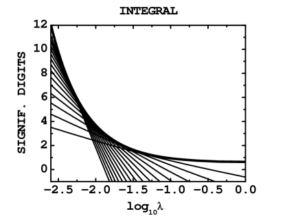
FIG. 1.: Number of significant digits versus $\lambda$ at order 1, 2, … 15. In all graphs, all the logs are in base 10. As the order increases, the curve rotates clockwise and moves left. The thick line is the envelope Eq. (5). The large blank area in the upper right corner is the region not accessible in regular perturbation theory.

A simple way to convert the asymptotic series into a converging one [7, 5] consists in restricting the range of integration to $|\phi|<\phi_{max}$. On the restricted domain, ${\rm e}^{-\lambda\phi^{4}}$ converges uniformly and one can then interchange legally the sum and the integral. We are then considering a modified problem namely the perturbative evaluation of

$$Z(\lambda,\phi_{max})=\int_{-\phi_{max}}^{+\phi_{max}}d\phi\ {\rm e}^{-(m^{2}/2)\phi^{2}-\lambda\phi^{4}}\ .$$ (7)

As the order increases, the peak of the integrand of $a_{k}$ (see Eq. (4)) moves across $\phi_{max}$ and the large order coefficients are suppressed by an inverse factorial: $|a_{k}|<\sqrt{2\pi}\phi_{max}^{4k}/k!$. At the same time, we have an exponential control of the error:

$$|Z(\lambda)-Z(\lambda,\phi_{max})|<2{\rm e}^{-\lambda\phi_{max}^{4}}\int_{\phi_{max}}^{\infty}d\phi\ {\rm e}^{-(m^{2}/2)\phi^{2}}\\$$ (8)

Everything works in a very similar way for other numerically solvable $\lambda\phi^{4}$ problems in $D=1$ (anharmonic oscillator) and $D=3$ (scalar field theory in the hierarchical approximation). The only difference being that in these two cases, a more demanding computational effort is required. This should be kept in mind while discussing the general strategy to be followed. If we could calculate as many perturbative coefficients as needed, an obvious strategy would be to pick a field cut $\phi_{max}$ large enough to satisfy some accuracy requirement. Then, given that the modified series is convergent, we could calculate enough coefficients to get an answer with the required accuracy. Unfortunately for any other problem than the integral, it is difficult to calculate the coefficients. A more realistic approach is to assume that we can only reach a fixed order and pick the field cutoff in such a way that at this order, we reach an optimal accuracy. Before doing this with a different procedure for even and odd orders as explained in the introduction, we will first discuss the strong coupling expansion of Eq. (1).

III Strong coupling expansion

In the following, we will often use the strong coupling expansion of the integral (1) and a few points should be clarified. Our original integral $Z(\lambda)$ vanishes in the limit where $\lambda\rightarrow\infty$. However $\lambda^{1\over 4}Z(\lambda)$ has a finite non-zero limit and can be expanded in powers $m^{2}/\lambda^{1/2}$:

$$\lambda^{1\over 4}Z(\lambda)=\sum_{l=0}^{\infty}(m^{2}/\lambda^{1/2}))^{l}b_{l}\ ,$$ (9)

with

$$b_{l}=(-1)^{l}(1/2)^{l+1}(1/l!)\Gamma(l/2+1/4)$$ (10)

This expansion is converging over the entire complex plane. However, if we look at the first few orders displayed later in Fig. 6, one might be tempted to conclude that the series has a finite radius of convergence because the curves representing the significant digits seem to have a “focus” near $\lambda\ =\ 10^{-1.5}$. To be completely specific, we mean that in Fig. 6, the four curves labeled S0 to S4 seem to intersect at a given point. However, as many more orders are displayed, the apparent focus moves left and a “caustic” (envelope) appears. This is shown in Fig. 2. The only difference with Fig. 1 is that the region which is inaccessible is now below. In other words, it is impossible to reach arbitrarily low accuracy using the strong coupling expansion!

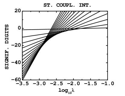
FIG. 2.: Number of significant digits versus $\lambda$ at order 1, 11, 21, … 141 in the strong coupling expansion. As the order increases, the curve rotates counterclockwise and moves left.

In lattice field theory, the strong coupling expansion is similar to the high temperature expansion and for $D>2$ we expect that the expansion has a finite radius of convergence due to the existence of a low temperature phase. This difference is not fundamental for the discussion which follows because we never use the large order contributions of the strong coupling expansion. Consequently, for any practical purpose, the situation will be similar to the case where we have a finite radius of convergence.

IV Even orders

If $\phi_{max}$ is the only adjustable parameter, the perfect choice is a solution of:

$$\int_{-\infty}^{+\infty}d\phi\ {\rm e}^{-(m^{2}/2)\phi^{2}-\lambda\phi^{4}}=\sum_{k=0}^{K}a_{k}(\phi_{max})\lambda^{k}\ ,$$ (11)

with

$$a_{k}(\phi_{max})={(-1)^{k}\over{k!}}\int_{-\phi_{max}}^{+\phi_{max}}d\phi\ {\rm e}^{-(m^{2}/2)\phi^{2}}(\phi^{4})^{k}$$ (12)

Below, we prove that this equation has no solution when $K$ is odd, and $K$ is assumed to be even in this section. This equation can be solved numerically with good accuracy using Newton’s method or a binary search. Our goal is to find approximate methods (which can be used in more complicated situations) to solve this equation and compare them with the accurate numerical solutions. In the rest of this section, we consider the cases of strong and weak coupling estimates of the optimal value of $\phi_{max}(\lambda)$.

A Strong Coupling Estimates

Multiplying both sides of Eq. (11) by $\lambda^{1/4}$ and expanding in powers of $m^{2}/\lambda^{1/2}$ we obtain at zeroth order that $\lambda\phi_{max}^{4}\simeq C_{K}^{(0)}$, with $C_{K}^{(0)}$ a solution of

$$4\sum_{k=0}^{K}(-1)^{k}{(C_{K}^{(0)})^{k+{1/4}}\over{k!(4k+1)}}=\Gamma({1/4})\ .$$ (13)

The solutions of this transcendental equation are displayed in Fig. 3 for various orders $K$. Asymptotically, $C_{K}^{(0)}\simeq 0.75+0.28K$. These solutions can be compared with the solutions $D_{K}$ of the equation

$${\rm e}^{-D_{K}}=(D_{K})^{K}/K!\ ,$$ (14)

which can be used as a rough estimate of $\lambda\phi_{max}^{4}$. Asymptotically, $D_{K}\simeq AK+\dots$, where $A=0.278465\dots$ is a solution the transcendental equation ${\em e}^{-A-1}=A$.

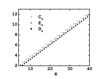
FIG. 3.: Solutions $C^{(0)}_{K},D_{K}$ and $E_{K}$ defined by Eqs. (13), (14) and, later in the text, by Eq. (20).

This lowest order (in the strong coupling) estimate of the optimal value of $\phi_{max}$ is quite good. In Fig. 4, we see that for $K$ = 6 it provides a significant improvement compared to the regular perturbative series at order 6 for $\lambda>10^{-2}$. In Fig. 4, we also compare with the accuracy at fixed cuts. For a fixed value of $\phi_{max}$, Eq. (11) has one solution for a given $\lambda$ and the accuracy becomes infinite at this value. In the Fig. we see only peaks of finite height, but we see that the approximation goes quite high in the peak, in other words, we localize the optimal value quite well.

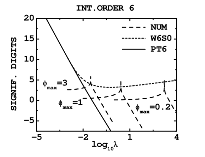
FIG. 4.: Significant digits obtained with the optimal cut $\phi_{max}(\lambda)$ estimated using a strong coupling expansion at lowest order (W6S0), compared to results at three fixed cuts and regular perturbation theory (PT6) at order 6.

We can now proceed to higher orders in $m^{2}/\lambda^{1/2}$ using the expansion

$$\lambda\phi_{max}^{4}=\sum_{l=0}C_{K}^{(l)}(m^{2}/\lambda^{1/2})^{l}\ ,$$ (15)

and plug it in the expansion in the same parameter of Eq. (11). The new coefficients obey linear equations which can be solved order by order. The optimal $\phi_{max}(\lambda)$ calculated at the four lowest orders in $m^{2}/\lambda^{1/2}$ are shown in Fig. 5. As explained in section III, below a certain value of $\lambda$ a few orders in the strong coupling expansion won’t help and one needs much higher order to improve the estimate in this region. After a short reflection, one can conclude that the “focus” observed in Fig. 6 is compatible with Fig. 5.

A few words should be said about the notations we use for the curves in the figures. When we write W6S1, this means that we use the weak coupling expansion up to order $K$=6 in Eq. (11)(this is the W6 part) and a strong coupling expansion at order 1 in $m^{2}/\lambda^{1/2}$ (this is the S1 part) in the calculation of the optimal $\phi_{max}$. In addition, PT8 means the 8th order in regular perturbation theory. In some figures, some of the indexes appear directly near the corresponding curve.

The accuracy of the truncated series at $\phi_{max}$ calculated with the higher order corrections in $m^{2}/\lambda^{1/2}$ in Fig 6. For comparison, the accuracy obtained by using only the strong coupling expansion Eq. (9). is also shown. The figure makes clear that the method proposed here represents a significant improvement compared to the separate use of the conventional weak and strong coupling expansions.

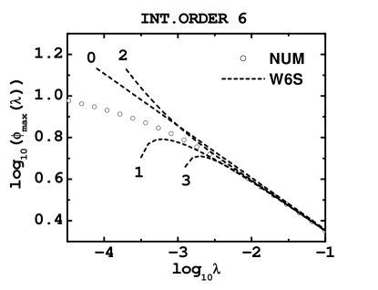
FIG. 5.: Estimates of the optimal $\phi_{max}(\lambda)$ at the first four orders in the strong coupling expansion

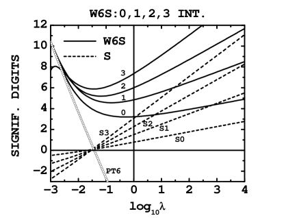
FIG. 6.: Significant digits obtained with the optimal cut $\phi_{max}(\lambda)$ (corresponding to a truncated expansion at order 6 in the weak coupling) estimated using the strong coupling expansion at orders 0, 1, 2 and 3 (solid lines), compared to significant digits using only the strong coupling expansion of the integral at the same orders in the strong coupling (dashed lines) and regular perturbation theory at order 6 (PT6).

B Weak coupling

As we learned in the previous subsection, as $\lambda$ decreases, the optimal value of $\phi_{max}$ increases. In the limit of a weak coupling, the “tails” of the integral that we removed become a small quantity. It is thus advantageous to split the l.h.s. of Eq. (11) into its bulk and tails and expand ${\rm e}^{-\lambda\phi^{4}}$ in the bulk where it is justified. The resulting (exact) equation for $\phi_{max}$ is then

$$2\int_{\phi_{max}}^{+\infty}d\phi\ {\rm e}^{-(m^{2}/2)\phi^{2}-\lambda\phi^{4}}=-\sum_{k=K+1}^{\infty}a_{k}(\phi_{max})\lambda^{k}\ ,$$ (16)

In the limit of very small $\lambda$, Eq. (16) becomes

$$(2/(m^{2}\phi_{max})){\rm e}^{-(m^{2}/2)\phi_{max}^{2}}\simeq-a_{K+1}\lambda^{K+1}\ .$$ (17)

The l.h.s. has a functional form similar to semi-classical estimates of the energy shifts in quantum mechanics [5, 10]. A more refined version of this equation is

$$2\int_{\phi_{max}}^{+\infty}d\phi\ {\rm e}^{-(m^{2}/2)\phi^{2}-\lambda\phi^{4}}\simeq-a_{K+1}(\phi_{max})\lambda^{K+1}\ ,$$ (18)

It is clear that the two above equations have solutions only when $K$ is even because in this case $a_{K+1}<0$. In Appendix A, it is shown that this property extends to the exact Eq. (11). More precisely the r.h.s. of Eq. (11) is positive for $K$ even and negative for $K$ odd.

Eq. (18) can be further improved by including higher order truncations at odd orders:

$$2\int_{\phi_{max}}^{+\infty}d\phi\ {\rm e}^{-(m^{2}/2)\phi^{2}-\lambda\phi^{4}}=-\sum_{k=K+1}^{K+3}a_{k}(\phi_{max})\lambda^{k}\ ,$$ (19)

and so on. In the following, we refer to the successive approximations defined by Eqs. (17), (18) and (19) as approximations $A1$, $A2$ and $A3$ respectively. The estimates of the optimal $\phi_{max}$ obtained with these approximations and the corresponding accuracies as a function of the coupling are shown in Figs. 7 and 8.

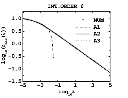
FIG. 7.: Estimates of the optimal $\phi_{max}(\lambda)$ obtained with the approximations $A1$, $A2$ and $A3$ defined in the text for $K$ = 6, compared to numerical values (empty circles).

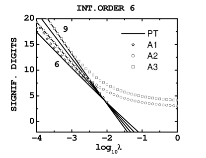
FIG. 8.: Significant digits obtained with the approximations $A1$, $A2$ and $A3$ for $K$ = 6, compared to order 6 to 9 in regular perturbation theory (solid lines rotating clockwise as the order increases).

One can see that A1 provides good estimates of $\phi_{max}$ optimal only at very small $\lambda$. On the other hand, A2 and A3 both provide good estimates even at large coupling. Not surprisingly, the accuracy of A2 (A3) merges with order 7 (9) in regular perturbation theory.

V Odd orders

As explained in section IV, for series truncated at odd $K$, the r.h.s. of Eq. (11) is negative. The best that we can do is to minimize the error (i. e., the difference between the r.h.s. and the l.h.s. . The minimization condition implies that $\lambda\phi_{max}^{4}=E_{K}$, the unique (see Appendix A, where $f_{K}$ is defined) solution of

$$\sum_{k=0}^{K}{(-E_{K})^{k}\over{k!}}=f_{K}(E_{k})=0\ .$$ (20)

In the following, we refer to this condition as the Principle of Minimal Sensitivity (PMS) condition. This terminology has been used [8] in the LDE where the variational parameter is fixed by requiring that the final estimate depends as least as possible on this parameter. The solutions $E_{K}$ are displayed in Fig. 3 which shows that they are asymptotically close to the solutions $C_{K-1}^{(0)}$ obtained at the lowest order in the strong coupling expansion. The accuracy obtained using the PMS condition is by construction the envelope of the accuracy obtained for all possible $\phi_{max}$. This is illustrated in Fig. 9.

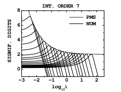
FIG. 9.: Significant digits obtained with the PMS condition compared to the same quantity at fixed cuts.

Nevertheless, an exact match between the original integral and the truncated perturbative expansion with a field cut can be obtained by using a mass shift $m^{2}\rightarrow m^{2}(1+\eta)$. Using obvious notations, we denote the cut integral defined in Eq. (7) with this mass shift $Z(\lambda,\phi_{max},\eta)$. The level curves of the perturbative expansion of $Z(\lambda,\phi_{max},\eta)$ at fixed $\lambda$ follow different patterns at odd and even orders as illustrated in Fig. 10.

At even order, all the level curves cross the $\eta=0$ line and there is no need for a mass shift. This case was discussed in section IV. At odd order, the level curve corresponding to the exact value $Z(\lambda)$ defines a curve $\eta(\phi_{max})$. In appendix B, we show that this curve stays in the half-plane $\eta<0$. We are now free to pick an arbitrary value of $\phi_{max}$ and adjust $\eta=\eta(\phi_{max})$. In the following we will pick $\phi_{max}$ in such a way that $\eta$ is as small as possible. This can be accomplished by solving the equation

$$\partial\eta/\partial\phi_{max}=0\ ,$$ (21)

for $\phi_{max}$. In appendix B, we show that this condition is indeed equivalent to the PMS condition (20) and consequently we have simply $\phi_{max}=(E_{K}/\lambda)^{1/4}$. With this choice, the introduction of $\eta$ is a natural continuation of the optimization at $\eta$ =0. Estimations of $\eta$ for this choice of $\phi_{max}$ can be obtained approximately at strong and weak coupling.

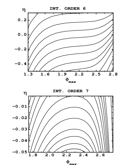
FIG. 10.: Level curves of the perturbative expansion of $Z(\lambda,\phi_{max},\eta)$ at order 6 and 7 in $\lambda$ evaluated at $\lambda=0.1$.

In the limit of arbitrarily small coupling, we can treat $\eta$ as a quantity of order $\lambda^{K+1}$ and use it to make up for the “missing” even contribution that would allow a solution of Eq. (11). This reasoning implies the weak coupling estimate

$$\eta\simeq-\lambda^{K+1}a_{K+1}(\phi_{max})m(2/\pi)^{1/2}$$ (22)

On the other hand, at strong coupling, $\eta$ grows like $\lambda^{1/2}$ and we need to expand

$$m^{2}\eta\lambda^{-1/2}=\sum_{l=0}^{\infty}B_{l}(m^{2}/\lambda^{1/2})^{l}\ .$$ (23)

The two approximation work well in their respective range of validity as shown in Fig. 11. The significant digits obtained with the various procedures are displayed in Fig. 12. One sees that the mass shift provides a significant improvement compared to the PMS condition at $\eta$=0. If we compare the two methods in their respective region of validity, the improvement provided by the strong coupling method is more substantial. Not surprisingly, W7W8 merges with PT8 at weak coupling.

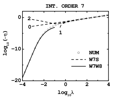
FIG. 11.: Optimal $\eta$ as a function of $\lambda$. Numerical values (empty circles) compared to approximate values obtained with the weak coupling expansion expansion (W7W8) corresponding to Eq. (22) with $K=7$ and the orders 0, 1 and 2 in the strong coupling expansion (W7S) from Eq. (23).

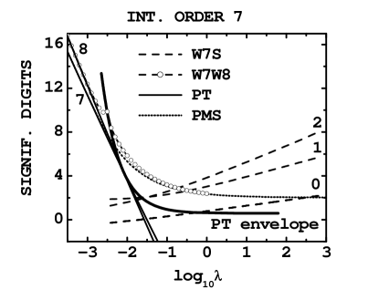
FIG. 12.: Significant digits for the same approximations as in Fig.11 compared to the regular perturbative series at orders 7 and 8 (thin solid line), the PMS result with $\eta$=0 at order 7 (small dots) and the envelope of regular perturbation theory (thick solid line).

We can now compare the accuracy of various estimates based on strong coupling expansions at the same order in $m^{2}/\lambda^{1/2}$. Examples are shown in Fig. 13 where the accuracy obtained with three methods relying on estimates at order one in $m^{2}/\lambda^{1/2}$ are displayed. One can see that as the coupling becomes large, the accuracy increases at the same rate in the three cases. As we already know in the even case, our method significantly improves the basic strong coupling expansion from Eq. (9). However, the improvement based on even order $K=2q$ in $\lambda$ performs significantly better than the improvement based on the odd order $K=2q+1$. Consequently, when in the next section we compare with other existing methods, we will restrict ourselves to the even case.

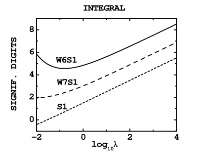
FIG. 13.: Significant digits obtained with the strong coupling expansion at order one in $m^{2}/\lambda^{1/2}$ and the approximations W6S1 and W7S1 discussed previously.

VI comparison with other methods

There exists several methods to improve the accuracy of asymptotic series. These include Padé’s approximants [6] applied to the series itself or its Borel-transform and the LDE [8]. These methods are compared among themselves in Fig. 14.

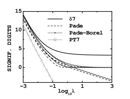
FIG. 14.: Comparison of the delta expansion at order 7 ($\delta 7$) with Padé approximants and the Padé-Borel method. In both cases the approximants [4/3], [3,4] and [2,5] have been used.

One can see that at weak coupling, the LDE provides an upper envelope for the accuracy while at strong coupling it prevails more significantly. Consequently, we only need to compare our results to the LDE. This is done in Fig. 15 where we see that at strong and moderate coupling, our methods provide a significant improvement compared to the LDE. On the other hand, at weak coupling, the improvements that we proposed, do not perform as well as the LDE.

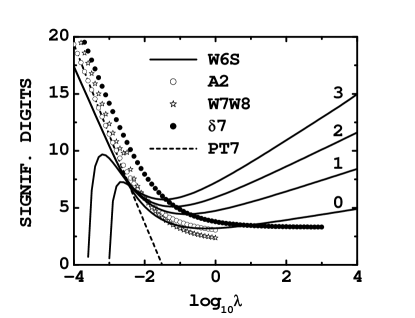
FIG. 15.: Comparison of the delta expansion at order 7 ($\delta 7$) with various methods discussed previously and regular perturbation at order 7 (PT7).

The results of Fig. 15 have been obtained by making the replacements [8] $m^{2}\rightarrow\Omega^{2}+\delta(m^{2}-\Omega^{2})$ and $\lambda\rightarrow\delta\lambda$. We then expanded the perturbative series at order $K$ in $\lambda$ to order $K$ in $\delta$. The arbitrary parameter $\Omega^{2}$ was determined by requiring that the derivative of the estimate with respect to $\Omega^{2}$ vanishes. This was called the PMS condition in Ref. [8] and it has a solution at odd orders only.

At even orders, it is however possible to proceed in a way similar to what we have done in subsection IV A, namely matching the strong coupling expansion of the estimate with the usual strong coupling of the integral in order to determine the arbitrary parameter. At order zero in $m^{2}/\lambda^{1/2}$, this results into a transcendental equation which has a solution at even orders only. Higher orders corrections to $\lambda/\Omega^{4}$ can then be calculated by solving linear equations just as in subsection IV A. The numerical results for $K=6$ are displayed in Fig. 16. One can see that this method and the method presented in subsection IV A have very similar accuracy at moderate and strong coupling.

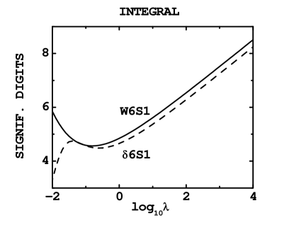
FIG. 16.: Significant digits obtained using the strong coupling expansion at order one in $m^{2}/\lambda^{1/2}$ to determine $\Omega$ in the $\delta$ expansion at order 6 compared the approximation W6S1 discussed previously.

The procedure we have used above is closely related to variational methods [9] where weak and strong coupling expansions were combined for various purposes. The only difference is that here we simply imposed the matching with the strong coupling expansion rather than resorting to extremization procedures or large order scaling arguments.

VII Conclusions

In conclusion, for even series in the weak coupling, the method which consists in determining the optimal value of $\phi_{max}$ using the strong coupling expansion provides excellent results at moderate at strong coupling. There is room for improvement at weak coupling. In particular, progress could be made by finding accurate approximations to calculate a large number of terms in the r.h.s. of Eq. (16).

The methods used here can be extended to quantum mechanics and in particular for the anharmonic oscillator where similar calculations have been partially performed[14]. We are planning to apply the methods developed here for higher dimensional SFT where the LDE seems to converge very slowly [11] (see also [12, 13] for methods to improve the situation). One difficulty is to calculate the perturbative coefficients with a field cutoff. Monte Carlo methods have been recently developed for this purpose [15].

This research was supported in part by the Department of Energy under Contract No. FG02-91ER40664. Y. M. was at the Aspen Center for Physics while this work was in progress. Y. M. was partly supported by a Faculty Scholar Award at The University of Iowa and a residential appointment at the Obermann Center for Advanced Studies at the University of Iowa, while the manuscript was written.

A Non-existence of solutions in the odd case

In this appendix, we show that Eq. (11) has no solution when $K$ is odd. For this purpose we introduce the truncated exponential series:

$$f_{K}(x)=\sum_{k=0}^{K}(-1)^{k}x^{k}/k!\ ,$$ (A1)

and their complement

$$g_{K}(x)=\sum_{k=K}^{\infty}(-1)^{k}x^{k}/k!\ .$$ (A2)

Using the fact that $f^{\prime}_{K}=-f_{K-1}$ and a similar relation for the $g$, one can show by induction that for $K$ even, $f_{K}$ is strictly positive and $g_{K}$ is positive with its only zero at zero. For $K$ odd and $x>0$, $g_{K}$ is negative and decreases. Given that the r.h.s. of Eq. (16) is the integral with a positive measure of $-g_{K+1}$ over positive argument, we see that the r.h.s. is positive when $K$ is even and negative when $K$ is odd. Since the l.h.s. is always positive, they are no solutions for $K$ odd.

B Special Features of $\eta(\phi_{max})$

The function $\eta(\phi_{max})$ is the solution of the equation

$$Z(\lambda)=\int_{-\phi_{max}}^{\phi_{max}}{\rm e}^{-(m^{2}/2)(1+\eta(\phi_{max}))\phi^{2}}f_{K}(\lambda\phi^{4})\ .$$ (B1)

In this appendix, $K$ is assumed to be odd. For $x>0$, we have $f_{K}(x)<{\rm e}^{-x}$ because $g_{K+1}(x)>0$ for $K+1$ even and $x>0$ (see appendix A). We can compensate this underestimation by making the integration measure more positive, in other words picking the parameter $\eta<0$. The l.h.s. of Eq. (B1) is independent of $\phi_{max}$. Taking the derivative of Eq. (B1) with respect to $\phi_{max}$ and imposing that $\phi_{max}$ is a solution of $\partial\eta/\partial\phi_{max}=0$ , we obtain that for this special value of $\phi_{max}$, we have

$$f_{K}(\lambda\phi_{max}^{4}){\rm e}^{-(m^{2}/2)(1+\eta(\phi_{max}))\phi_{max}^{2}}=0\ .$$ (B2)

which implies the PMS condition (20).

REFERENCES

- [1] R. Feynman, Quantum Electrodynamics (Princeton University Press, Princeton, 1985).
- [2] A. Sirlin, eConf C990809, 398 (2000).
- [3] F. Dyson, Phys. Rev. 85, 32 (1952).
- [4] J. C. Le Guillou and J. Zinn-Justin, Large-Order Behavior of Perturbation Theory (North Holland, Amsterdam, 1990) ands Refs. therein.
- [5] Y. Meurice, Phys. Rev. Lett. , 88, 141601 (2002).
- [6] G. Baker and P. Graves-Morris, Padé Approximants (Cambridge University Press, Cambridge, 1996).
- [7] S. Pernice and G. Oleaga, Phys. Rev. D 57, 1144 (1998).
- [8] I. R. C. Buckley, A. Duncan, and H. F. Jones, Phys. Rev. D 47, 2554 (1993); C. Bender, A. Duncan, and H. F. Jones, Phys. Rev. D 49, 4219 (1994); R. Guida and K. Konishi and H. Suzuki, Annals of Physics 241, 152 (1995) and 249, 109 (1996).
- [9] H. Kleinert, Phys. Lett. A 207, 133 (1995); W. Janke and H. Kleinert, Phys. Rev. Lett. 75, 2787 (1995).
- [10] L. Li and Y. Meurice, Nucl. Phys. Proc. Suppl. 119 873-875. (2003).
- [11] E. Braaten and E. Radescu, Phys. Rev. Lett. 89, 271602 (2002).
- [12] J.-L. Kneur, M. Pinto, and R. Ramos, Phys. Rev. Lett. 89, 210403 (2002).
- [13] B. Hamprecht and H. Kleinert, hep-th/0302116.
- [14] B. Kessler, L. Li and Y. Meurice, work in progress.
- [15] L. Li and Y. Meurice, “The Continuum Limit of Perturbative Coefficients Calculated with a Large Field Cutoff”, Talk given at Lattice 2003, Tsukuba, hep-lat/0309xxx.