Warped Strings: Self-dual Flux and Contemporary Compactifications

Abstract

String theory is a leading candidate for the quantum theory of gravitation and is the only serious unified theory of all the forces of physics. Additionally, string theory seems to be mathematically unique, and it is possible that all the parameters of physics could be determined by the dynamics of string theory. However, there are two intertwined problems. First is that string theory requires ten dimensions for mathematical consistency, so six must be compact or otherwise decoupled from the physics we observe. Also, there exist many different ground states of string theory, so it is difficult to make predictions that are generic to string theory. Therefore, it is crucial to gain a broad understanding of all the string theory vacua, particularly those compactified to four dimensions.

In recent years, our understanding of string theory compactifications has expanded greatly to include many new classes of solutions. In this dissertation, I discuss type IIB string compactifications in which the three-form field strengths satisfy a self-duality condition on the internal manifold. I begin with an overview of the models, giving preliminary formulae and several points of view from which they can be understood. Then I will describe windows into the small radius behavior of the compactifications, which is more complicated than compactifications without fluxes, which are more well-known. I will describe details of the flux-generated potential and nonperturbative corrections to it. These nonperturbative corrections allow a discussion of the cosmological constant and possible mechanisms for the universe to decay from one energy state to another. I conclude with comments on related topics and interesting directions for future study.

As this document is a dissertation, I will indicate my own contributions to the subject. However, for the purpose of completeness and in hopes of helping the readers, I will include a fairly comprehensive review of related literature. The early part of the dissertation is much more a literature review because there are many results upon which my contributions have been founded.

Acknowledgements

First of all, I thank the faculty who have influenced my education, including Omer Blaes and Claudio Campagnari for various forms of support. Particularly I thank the string theory faculty, Steven Giddings, David Gross, Gary Horowitz, and Joseph Polchinski, for encouragement and instruction. Especially I thank my advisor, Joseph Polchinski, for guidance. Not only has he taught me a great deal of physics, but he has also ensured that I had the necessary support to get through difficult times. I am very grateful to have had him for a mentor.

I would also like to thank the many people with whom I have had interesting discussions. Specifically, I have benefited greatly from UCSB graduate students and postdocs, including I. Bena, O. deWolfe, H. Elvang, T. Erler, S. Hellerman, V. Hubeny, A. Maharana, and N. Mann. Outside of UCSB, I have benefited from discussions with E. D’Hoker, S. Ferrara, S. Kachru, M. Schulz, and E. Silverstein. I would especially like to thank my collaborators, A. Buchel, M. Graña, M. Lippert, A. Mazumdar, and B. Williams.

For financial support, I am grateful to the National Science Foundation and the UCSB Physics Department and Graduate Division. Part of my work has been supported through UCSB fellowships and an NSF Graduate Research Fellowship.

Finally, I thank my family for much support throughout my entire education and life. Most importantly, I thank my wife, Rebecca Danos, whose love and support have helped me through every aspect of my life.

Chapter 1 General Theory

This chapter gives some motivational words along with an introduction to the compactifications that are the subject of this dissertation.

1.1 Introduction

The Standard Model of particle physics is, by all accounts, remarkably successful in that it is very well corroborated by experiment (with the exception of neutrino mixing), so much so that it is almost universally capitalized in spelling and pronunciation. However, theorists have long been frustrated by the number of parameters in the Standard Model, such as gauge couplings and the Yukawa couplings that determine fermion masses. Naturally, there have been many attempts to extend the Standard Model to a theory that predicts those parameters.

Possibly the most promising of the attempts has been string theory, a reformulation of particle physics in terms of extended one dimensional objects, or strings. One of the great advantages of string theory is that all of its parameters are dynamical variables, so presumably all the parameters of the Standard Model can be determined by finding the ground state of all those variables in string theory. Unfortunately, there are an incredible number of ground states of string theory, and, through the turn of the century, the best understood of these vacuum states allow many of the parameters, or moduli, to take on a continuum of values. This problem of free moduli is related to the number of ways to compactify string theory from ten dimensions (necessary for the mathematical consistency of the theory) to the four dimensions in which we live.

Starting just before the new millenium, though, string theorists have developed mechanisms for fixing the values of moduli in a number of different contexts (as it turns out, some of these mechanisms are related). In this document, I review the dimensional reduction of type IIB string theory from ten to four dimensions, with an emphasis on the use of rank 3 field strengths to freeze moduli. A particular feature of these models is that the field strengths must satisfy a self-duality condition on the compact space, so I will often call them self-dual fluxes. This first chapter will give the general theory of such compactifications, including the solution of type IIB supergravity, and the second will find the effective four dimensional theory from several perspectives. The discussion of the first two chapters will mainly be valid at large volumes for the compact six dimensions; in a subsequent chapter, I will consider the small volume regime. Later, I will discuss the application of these models to cosmological issues (chapter 4) and some open questions (chapter 5).

Throughout, I will give particular attention to work to which I have made a contribution in the course of graduate study. The papers to which I have contributed relevant to this review are [1, 2, 3, 4, 5, 6]. Results from them appear as follows:

• Results from [1] are scattered throughout the dissertation, in sections 2.1, 2.3.1, 3.1, 3.2.1, and 3.3.1. Some results which were derived in preparation for [1] but not previously published also appear in section 2.1.

• The counting of BPS states from [2] appears in section 3.2.2.

• The cosmology discussed in section 4.1 is from [3].

• The discussion of [4] regarding string corrections and symmetry breaking is included, in condensed form, in section 5.2.1.

• The explicit description of de Sitter vacua given in [5] appears in section 4.3.1, while the calculations of decay times from that paper appear in 4.3.2.

• The supersymmetric solutions that will appear in [6] are given in section 1.3.2.

Appendix A discusses the conventions and notation that I use. Actions and equations of motion are given in appendix B. Some derivations that are too detailed for the main text are collected in appendix C.

1.2 Phenomenological Motivation

To start, it is probably useful to review the basic phenomenological models that inspired some of the recent developments in string compactifications. This section is mainly intended as a short motivation, along with the idea of moduli stabilation discussed above, for the more specific results developed later.

The first major development was the implication that the Standard Model might be confined to a brane, or domain wall, so that only gravity could move through some number of extra dimensions; since gravity is very poorly measured in comparison to the Standard Model, the extra dimensions can be fairly large before giving problems due to graviton Kaluza-Klein modes [7, 8, 9]. An exciting feature of these models is that the large extra dimensions can allow the 4D Planck scale to be much higher than the extra dimensional Planck scale; taking the metric on the internal compact space to be fixed, the reduction of the Einstein-Hilbert action is (up to convention dependent factors of $2\pi$, etc)

$$M_{D}^{D-2}\int d^{D}x\sqrt{-g_{D}}R=\left(M_{D}^{D-2}V_{D-4}\right)\int d^{4}x\sqrt{-g_{4}}R\Rightarrow M_{4}^{2}=M_{D}^{D-2}V_{D-4}\ .$$ (1.1)

(We will also use the gravitational coupling, $\kappa_{D}^{2}=1/M_{D}^{D-2}$, to represent the Planck scale.) Branes are very natural objects in string theory, and the Standard Model braneworld was identified with D-branes of string theory [10]. As long as the compactification length scale is large compared to the fundamental length scale of the higher dimensional theory, the 4D Planck scale can be quite large.

The next discovery was the importance of non-factorizable geometry; the traditional compactification ansatz is that the metric is just a direct product of the internal space and the noncompact spacetime. However, that is not the most general ansatz for a Poincaré invariant ground state; the metric

$$ds^{2}=e^{2A(x^{m})}\eta_{\mu\nu}dx^{\mu}dx^{\nu}+g_{mn}dx^{m}dx^{n}$$ (1.2)

is fully consistent with the Poincaré group. Here and henceforth, we use Greek indices $\mu,\nu,\cdots$ for the noncompact spacetime, and Latin $m,n,\cdots$ for the compact dimensions. In two simple models (with one and two branes), [11, 12] showed that the warp factor modifies the Kaluza-Klein decomposition, localizing the graviton zero-mode near one of the branes. In fact, [12] showed that infinitely large extra dimensions can still give rise to four dimensional effective theories of gravity due to this effect. These simplest models are five dimensional, compactified on $S^{1}/\bm{\mathbbm{Z}}_{2}$ with one brane at each fixed point, and a negative bulk cosmological constant that generates the warp factor. The focus of this document is on string compactifications that reproduce the physics of this simple two-brane model [13, 14].

What exactly does the four dimensional graviton look like? As it turns out, for the simple models of [11, 12], the zero mode graviton is just $\delta g_{\mu\nu}=e^{2A(x^{m})}h_{\mu\nu}(x^{\mu})$. In fact, the graviton takes precisely this form for a wide class of stress tensors [15], and it is known to have this form for the self-dual flux compactifications which I discuss in the rest of this review [16]; section 2.1 will give a demonstration. In terms of the effective theory of the light modes, then, the Planck constant (1.1) essentially picks up an additional $e^{2A}$ due to the rescaling of the 4D metric.

To put things more precisely, consider a compactification of string theory. The gravitational action of all string theories is, in the string frame,

$$S = \frac{1}{2\kappa_{10}^{2}}\int d^{10}x\sqrt{-g_{10}}e^{-2\phi}R_{10}=\frac{1}{2\kappa_{10}^{2}}\int d^{10}x\sqrt{-g_{4}}e^{2A}e^{6u}e^{-2\phi}R_{4}\ \$$ (1.3)

$$ds^{2} = e^{2A}g_{4,\mu\nu}dx^{\mu}dx^{\nu}+\cdots$$ (1.4)

where $e^{6u}$ gives the volume of the compact metric (other metric perturbations preserve volume) and where $2\kappa_{10}^{2}=(2\pi)^{7}\alpha^{\prime}{}^{4}$ (see, for example, [17]). Clearly, equation (1.3) does not give the usual Einstein-Hilbert term for $g_{4,\mu\nu}$; instead, we must convert to the 4D Einstein frame metric

$$g_{E,\mu\nu}=e^{6u}e^{-2\phi}g_{4,\mu\nu}$$ (1.5)

to decouple the dilaton and the overall volume of the compactification. Then the effective action is the usual

$$S=\frac{1}{2\kappa_{4}^{2}}\int d^{4}x\sqrt{-g_{E}}R_{E}\ ,\ \ \frac{1}{\kappa_{4}^{2}}=\frac{V_{w}}{\kappa_{10}^{2}}\ ,\ \ V_{w}=\int d^{6}x\sqrt{\det g_{mn}}\,e^{2A}e^{-6u}\ .$$ (1.6)

Note that now there can be a large hierarchy between 10D and 4D Planck constants due to a large warp factor. This particular form of the relation between Planck constants is due to [18].

What does this mean for the gauge/gravity hierarchy? Consider a Higgs scalar that lives on, for example, a D3-brane, with some string frame mass $m$ (ie, a fundamental mass $m$), much as in [11, 18]. In the string frame, the action (rescaling the D3 tension into the scalar to get canonical normalization) is

$$S=-\frac{1}{2}\int d^{4}xe^{-\phi}\sqrt{-g_{4}}e^{4A}\left[e^{-2A}\partial_{\mu}H\partial^{\mu}H+m^{2}H^{2}\right]\ .$$ (1.7)

We can already see that the mass as measured by the 4D effective theory is modified by a factor of $e^{2A}$, and going to the Einstein frame gives

$$S=-\frac{1}{2}\int d^{4}x\sqrt{-g_{E}}e^{\phi-6u+2A}\left[\partial_{\mu}H\partial^{\mu}H+e^{2\phi-6u+2A}m^{2}H^{2}\right]\ .$$ (1.8)

So the Higgs mass, compared to the Planck mass, measured by an observer on the brane is

$$\frac{m_{H}^{2}}{M_{4}^{2}}=e^{2\phi-6u+2A}(\textnormal{SM})\frac{m^{2}}{M_{10}^{8}V_{w}}\ .$$ (1.9)

So we can get a large hierarchy in a number of ways:

1. Weakly coupled strings

2. A large compactification volume ($u$ large), as in equation (1.1)

3. A small warp factor $e^{A}$ at the brane

4. $m\ll M_{10}$ for some reason such as supersymmetry

5. $m\sim M_{10}$, but large warped volume compared to $1/M_{10}^{6}$

or some combination of those. In fact, some of these reasons are essentially identical. For example, the first reason is not often discussed because it does not appear in the 10D Einstein frame; the relations (A.11,A.13) mean that the string coupling rescales the compactification volume and the fundamental mass. Also, its always possible to scale the coordinates so the warp factor is $1$ at the Standard Model brane, so the third and fifth reasons are identical. I will use the convention that, at large compactification radii, $A\sim 0$ away from special points such as a Standard Model brane. An important question is how the warp factor can be given a fixed small value near the Standard Model brane (in other words, how does the geometry develop a large hierarchy?), and the first phenomenological answer was given in [19, 20].

Similar considerations apply to other mass scales [18]; an observer on the Standard Model brane always sees a mass rescaled by the warp factor relative to the warp factor on the brane (similar considerations would apply to a varying dilaton). For example, a Kaluza-Klein mode could be localized in some region of the bulk, or supersymmetry could be broken on a different brane. Then

$$m^{2}(\textnormal{SM observed})=\frac{e^{2A}(\textnormal{KK/SUSY/etc.})}{e^{2A}(\textnormal{SM})}m^{2}(\textnormal{fundamental})\ .$$ (1.10)

A number of warped compactifications of string theory were discussed in [21] from the point of view of using the warp factor to generate large hierarchies. In the rest of this disseration, I will discuss another type of string compactification, type IIB strings with 3-form fluxes. In some instances, the fluxes can give large ratios of warp factors, and they always freeze many of the moduli.

1.3 Ten Dimensional Supergravity

Based on the supersymmetry variation of the gravitino in M-theory, [22] first studied compactifications of 11D supergravity to 3D with nonvanishing 4-form field strengths. Then, [23] explored duals of these compactifications in type IIB and heterotic string theory, mainly focusing on some simple examples, and [16] described the compactifications with fluxes as warped compactifications, paying special attention to the effect of the warp factor and fluxes on the dimensional reduction. In fact, [13, 14] argued that similar string compactifications could implement the models of [11]; the Standard Model would live on D-branes in a region of low warp factor, and the 6D compactification manifold would play the role of the second brane. More complicated type IIB compactifications appeared in [24], which also showed how to stabilize the warp factor at small values near special points.

In the next subsection, I will describe the full ten dimensional solution of type IIB string theory with self-dual flux, mainly following the discussion in [24]. Then, in 1.3.2, I review the fermion supersymmetry variations of type IIB supergravity and show which of the self-dual flux backgrounds are supersymmetric (at tree level), as well as exploring other relevant solutions.

Historical Note

Before launching into the actual compactifications that we will study, it might be useful to note a few early studies of fluxes in string compactifications [25, 26, 27, 28, 29, 30]. These papers introduced fluxes to Calabi-Yau compactifications, but most of them did not account for the importance of string theoretic objects such as orientifold planes, which we will develop below. However, they did develop an understanding of the role of fluxes in compactifications and provided motivation for the self-dual flux compactifications we review here.

In brief, [25] introduced fluxes in type IIA compactifications, studying the flux-induced scalar potential using the language of 4D $\mathcal{N}=2$ supergravity, and [26] extended this work to type IIB supergravity. The role of fluxes in string dualities was studied in [29]; [27, 28, 30] detailed various aspects of the potential. It is worth noting that [30] found that fluxes create a runaway potential toward infinite volume on the compactification manifold; presumably this effect arises because of the need for negative tension objects such as orientifold planes.

1.3.1 Solution to Equations of Motion

Type IIB string theory reduces in the low energy limit to 10D type IIB supergravity (SUGRA). The fields of IIB SUGRA are the metric, a complex scalar, two 3-form field strengths, and a self-dual 5-form field strength. The dilaton-axion scalar $\tau=C_{0}+ie^{-\phi}$ combines the RR scalar with the string coupling; thre is a $SL(2;\bm{\mathbbm{Z}})$ S-duality that takes $\tau\to(a\tau+b)/(c\tau+d)$. It is often convenient to combine the R-R ($F_{3}=dC_{2}$) and NS-NS ($H_{3}=dB_{2}$) 3-forms into a single complex field $G_{3}=F_{3}-\tau H_{3}$ that transforms as $G_{3}\to G_{3}/(c\tau+d)$ . The 5-form $\tilde{F}_{5}=dC_{4}-C_{2}H_{3}$ is neutral under S-duality, and self-duality $\star\tilde{F}_{5}=\tilde{F}_{5}$ is imposed as an equation of motion. I work in the 10D string frame; much of the literature uses 10D Einstein frame (see appendix A.3).

As in equation (1.2), we will take the most general Poincaré invariant metric, although we find it convenient to scale the warp factor out of the compact metric, as well. We take as a fairly general ansatz

$$ds^{2} = e^{2A}\eta_{\mu\nu}dx^{\mu}dx^{\nu}+e^{-2A}\tilde{g}_{mn}dx^{m}dx^{n}\ \textnormal{and}$$ (1.11)

$$\tilde{F}_{5} = e^{-4A}\epsilon_{(4)}dF-e^{-4A}\star_{(6)}dF\ ,$$ (1.12)

with $F_{3},H_{3}$ harmonic and $\tau$ satisfying its equations of motion. The warp factor in the 5-form ensures that $\tilde{F}_{\mu\nu\lambda\rho m}$ is closed, as required by the Bianchi identity (B.15) given in appendix A.3 along with the other equations of motion. As is consistent with Poincaré invarience, no fields vary in the spacetime.

A SUGRA No-Go Theorem and a Stringy Evasion

In examining the equations of motion for the metric, we will find the following $D$ dimensional identities very helpful:

$$\bar{g}_{MN} = e^{2\omega}g_{MN}\Rightarrow$$

$$\bar{R}_{MN} = R_{MN}-(D-2)\nabla_{M}\nabla_{N}\omega+(D-2)\nabla_{M}\omega\nabla_{N}\omega$$ (1.13)

$$-g_{MN}\nabla^{2}\omega-(D-2)g_{MN}\left(\nabla\omega\right)^{2}$$

$$\bar{\nabla}^{2}\psi = e^{-2\omega}\nabla^{2}\psi+(D-2)e^{-2\omega}\nabla^{P}\omega\nabla_{P}\psi\,,\ \psi\ \textnormal{scalar}\ .$$ (1.14)

In particular, for the metric (1.11), the rescaling (1.14) means that the 10D Laplacian $\nabla^{2}$ is equal to the 6D Laplacian $e^{2A}\tilde{\nabla}^{2}$ acting on scalars independent of $x^{\mu}$. To see that, remember that $\nabla^{2}$ has a term $-g^{\mu\nu}\Gamma^{m}_{\mu\nu}\partial_{m}$ and that $\Gamma^{m}_{\mu\nu}=-g_{\mu\nu}\nabla^{m}A$.

The spacetime components of the Ricci tensor of equation (1.11) are

$$R_{\mu\nu}=-\eta_{\mu\nu}e^{4A}\tilde{\nabla}^{2}A\ ,$$ (1.15)

where $\tilde{\nabla}$ is the covariant derivative with respect to the six dimensional metric $\tilde{g}_{mn}$ [24]. One way to find equation (1.15) is to use (1.13) with metric (1.11); take $\bar{R}_{\mu\nu}$ from (1.11), and use $e^{-2A}$ times (1.11) on the right-hand side. That metric has $\Gamma^{m}_{\mu\nu}=0,R_{\mu\nu}=0$, and rescaling the Laplacian back gets rid of the extra terms in (1.13).

The spacetime components of Einstein’s equation (B.13) can be written as

$$R_{\mu\nu} = -\frac{1}{4}g_{\mu\nu}\nabla^{2}\phi+\frac{1}{2}g_{\mu\nu}\nabla_{m}\phi\nabla^{m}\phi-2\nabla_{\mu}\nabla_{\nu}\phi-g_{\mu\nu}\frac{e^{2\phi}}{48}G_{mnp}\bar{G}^{mnp}$$ (1.16)

$$+\frac{1}{24}e^{2\phi}\tilde{F}_{\mu\lambda\rho\sigma\tau m}\tilde{F}_{\nu}{}^{\lambda\rho\sigma\tau m}+\kappa_{10}^{2}e^{2\phi}\left(T^{\prime}_{\mu\nu}-\frac{1}{8}g_{\mu\nu}T^{\prime M}_{M}\right)\ .$$

The local contributions, denoted by primes, represent string theoretic objects, such as D-branes and orientifold planes; note that the stress tensor contribution is multiplied by $e^{2\phi}$ due to the prefactor of the Hilbert term in the string frame action. The $\nabla_{\mu}\nabla_{\nu}\phi$ terms is nonvanishing because of the nontrivial Christoffel symbol $\Gamma^{M}_{\mu\nu}$. Remembering that the gradient on the dilaton is the full 10D derivative, we can rewrite (1.16) to

$$e^{4A}\tilde{\nabla}^{2}\left(A-\frac{\phi}{4}\right)\!\! =\!\! -\frac{1}{2}e^{4A}(\tilde{\nabla}\phi)^{\tilde{2}}+2e^{4A}\tilde{\nabla}^{m}A\tilde{\nabla}_{m}\phi+\frac{e^{2\phi}}{48}e^{2A}G_{mnp}\bar{G}^{mnp}$$ (1.17)

$$+\frac{e^{2\phi-6A}}{4}\partial_{m}F\partial^{m}\!F+\frac{\kappa_{10}^{2}}{8}e^{2A+2\phi}\left(T^{\prime m}_{m}-T^{\prime\mu}_{\mu}\right)$$

after tracing by $\eta^{\mu\nu}$. (Here $T^{\mu}_{\mu}$ has indices raised by the full string frame metric including warp factor.) Rescaling to a metric $\hat{g}_{mn}=e^{-\phi}\tilde{g}_{mn}$ gives

$$e^{4A-\phi}\hat{\nabla}^{2}\left(A-\frac{\phi}{4}\right) = \frac{e^{2\phi}}{48}e^{2A}G_{mnp}\bar{G}^{mnp}+\frac{e^{2\phi}}{4}e^{-6A}\partial_{m}F\partial^{m}F$$ (1.18)

$$+\frac{\kappa_{10}^{2}}{8}e^{2A+2\phi}\left(T^{\prime m}_{m}-T^{\prime\mu}_{\mu}\right)\ .$$

As was noted in [24], this equation demonstrates the SUGRA no-go theorem of [31, 32] directly in IIB supergravity; without the (purely stringy) local contributions, the right-hand side is positive definite, while the left-hand side integrates to zero on a compact manifold.

In fact, for a $p$-brane extendend through the entire spacetime and wrapped on a submanifold $\Sigma$ of the compact space, the local contribution to the stress tensor gives

$$\left(T^{m}_{m}-T^{\mu}_{\mu}\right)=(7-p)T_{p}\delta(\Sigma)\ ,$$ (1.19)

where $T_{p}$ is the $p$-brane tension [24]. Therefore, to get a negative contribution to the right-hand side of (1.18), there must either be branes with $p>7$ or negative tension objects. In type IIB string theory, both D9-branes and negative tension orientifold planes are stable objects. From here on, we will focus on the orientifolds.

Stringy Constraints

Gauss’s law assures us that the charges for all the field strengths must integrate to zero over the compact manifold. We are particularly interested in D3-brane charge, where Gauss’s law comes from the 5-form Bianchi identity (B.15). In fact, we can obtain both local and global constraints on the compactification from the Bianchi identity.

Local Constraints

Consider first the derivative side of the Bianchi identity. The components with spacetime indices are trivial, so we consider the part with only internal indices. If we Hodge dualize on it using the string frame metric in 6D, the derivative part becomes

$$\star_{(6)}d\tilde{F}_{5} = -\star_{(6)}d\left(e^{-4A}\star_{(6)}dF\right)=-e^{6A-3\phi}\hat{\star}_{(6)}d\left(e^{-8A+2\phi}\hat{\star}_{(6)}dF\right)$$ (1.20)

$$= e^{-2A-\phi}\hat{\nabla}^{2}F-2e^{-2A-\phi}\partial^{\hat{m}}\left(4A-\phi\right)\partial_{m}F$$

Then the entire Bianchi identity becomes

$$\hat{\nabla}^{2}F = \frac{i}{12}e^{2A+2\phi}G_{mnp}\left(\star_{(6)}\bar{G}\right)^{mnp}+2\kappa_{10}^{2}\mu_{3}e^{2A+\phi}\star_{(6)}\rho_{3}$$ (1.21)

$$+2e^{-6A+2\phi}\partial^{m}F\partial_{m}\left(e^{4A-\phi}\right)$$

where $\rho_{3}$ is the charge density 6-form of D3-branes (normalized to $1$ for a single brane) [24].

Now rewrite equation (1.18) as an equation for the second derivative of $e^{4A-\phi}$ and subtract equation (1.21). With some algebraic rearrangement,

$$\hat{\nabla}^{2}\left(e^{4A-\phi}-F\right) = \frac{e^{2A+2\phi}}{2}\left|iG-\star_{(6)}G\right|^{2}+e^{-6A+2\phi}\left|\partial\left(e^{4A-\phi}-F\right)\right|^{2}$$ (1.22)

$$+\frac{1}{2}\kappa_{10}^{2}e^{2A+2\phi}\left(T^{\prime m}_{m}-T^{\prime\mu}_{\mu}-4\mu_{3}e^{-\phi}\star_{(6)}\rho_{3}\right)\ .$$

Consider the last term of this equation. According to equation (1.19), this term vanishes for a D3-brane, since the tension and charge for D-branes are related by $T_{p}=\mu_{3}e^{-\phi}$ (and the number density is clearly given by the delta function). As in [24], make the assumption that all the local sources satisfy the inequality

$$T^{\prime m}_{m}-T^{\prime\mu}_{\mu}\geq 4\mu_{3}e^{-\phi}\star_{(6)}\rho_{3}\ .$$ (1.23)

This inequality is valid for D3-branes and $\overline{\textnormal{D3}}$-branes, as well as O3-planes and fractional D3-branes. Of these, only $\overline{\textnormal{D3}}$-branes do not saturate it because they have a negative D3-brane charge density. 7-branes can have an induced D3-brane charge due to worldvolume curvature and field strengths (from $\alpha^{\prime}$ corrections to the action, discussed more fully in SECTION), and [24] argued that they in fact saturate (1.23). We are, however, ruling out D5-branes and O5-planes; those must appear in some other class of solutions.

With the inequality (1.23), the three terms on the right hand side of (1.22) are positive definite, while the left hand side integrates to zero. This is the no-go theorem of [24]: for solutions with only local objects that obey (1.23), the 3-form is imaginary self-dual

$$iG_{3}=\star_{(6)}G_{3}\Rightarrow e^{-\phi}\star_{(6)}H_{3}=-\tilde{F}_{3}\,,\ \star_{(6)}\tilde{F}_{3}=e^{-\phi}H_{3}\ ,$$ (1.24)

the potential energy of a D3-brane cancels between the DBI and WZ parts (D3-branes feel no force)

$$F=e^{4A-\phi}\ ,$$ (1.25)

and the inequality (1.23) is saturated. Because the D3-branes feel no forces, we might expect that these solutions are related to supersymmetric solutions, and, indeed, all the localized sources that saturate the bound preserve the same SUSYs. We will see in the next section, 1.3.2, which fluxes also preserve SUSY.

We should also mention that the constraints and equation (1.21) lead to Poisson’s equation for the warp factor:

$$-\hat{\nabla}^{2}e^{-(4A-\phi)}=\frac{1}{12}e^{\phi}G_{mnp}\bar{G}^{\widehat{mnp}}+2\kappa_{10}^{2}\mu_{3}\hat{\star}_{(6)}\rho_{3}\ .$$ (1.26)

This equation tells us that the warp factor becomes trivial in the large radius limit (except at special points), as follows. If we scale $\hat{g}_{mn}\to e^{2u}\hat{g}_{mn}$, then the left hand side goes as $e^{-2u}$, while the right hand side goes as $e^{-6u}$. Therefore, the warp factor (combined with the dilaton) becomes a constant, which we take to be unity. So in a case where self-duality of the flux (1.24) freezes the dilaton, $A\sim e^{-4u}$.

With all of these conditions satisfied, we only need to discuss the metric $\tilde{g}_{mn}$, 3-form, and dilaton-axion. The simplest model is that the dilaton and axion are constant, in which case $\tilde{g}_{mn}$ is a (orientifolded) CY 3-fold. Then the 3-form equations of motion (B.16) are satisfied by closed 3-forms as long as equations (1.24,1.25) hold. The case of nonconstant $\tau$ is more complicated. It has been shown in [24] that these form a compactification of F-theory (given here in the IIB string frame) on a CY 4-fold. In F-theory, $\tau$ represents the complex structure of a $T^{2}$, and the degeneration points of the torus are $(p,q)$7-branes. These 7-branes can be described in string perturbation theory when particular combinations of them coincide. This is the “orientifold limit” of F-theory in which each O7-plane is coincident with 4 D7-branes, precisely enough so that the D7-brane charge cancels locally [33]. In the orientifold limit, $\tau$ becomes a constant once again.

Global Constraints

Constraints global on the compactification manifold arise from integrating the Bianchi identity (B.15). If the F-theory 4-fold has Euler number $\chi$, the integrated Bianchi identity becomes [22, 34]

$$\frac{\chi}{24}=N_{\textnormal{D3}}-\frac{1}{4}N_{\textnormal{O3}}+\frac{1}{4}N_{\widetilde{\textnormal{O3}}}+\frac{1}{2\kappa_{10}^{2}\mu_{3}}\int H_{3}\wedge F_{3}\ .$$ (1.27)

Here $N_{\textnormal{O3}}$ is the number of “regular” O3-planes and $N_{\widetilde{\textnormal{O3}}}$ the number of O3-planes with flux discussed below under the quantization of fluxes. Both [34, 24] argued that $-\chi/24$ is the complete D3-brane number induced on 7-branes through $\alpha^{\prime}$ corrections to F-theory (or, rather, the D-brane action in string theory). We have left off $\overline{\textnormal{D3}}$-brane number because anti-branes do not saturate the inequality (1.23).

Let us also note that this equation is a nonperturbative generalization of worldsheet tadpole cancellation conditions, which are necessary for consistency of the string theory (just as the integrated Bianchi is a geometric consistency condition). Hence we will sometimes refer to the integrated Bianchi in terms of tadpole cancellation.

Orientifold Projections

There are two types of orientifold planes that could appear in the self-dual flux compactifications, as discussed above.

O3-planes

If the compactification manifold has a reflection symmetry of all compact coordinates $x^{m}$,

$$R:\quad(x^{4},x^{5},x^{6},x^{7},x^{8},x^{9})\to(-x^{4},-x^{5},-x^{6},-x^{7},-x^{8},-x^{9})\ ,$$ (1.28)

it can be orientifolded by placing O3-planes at the fixed points.

The action of the orientifold $\bm{\mathbbm{Z}}_{2}$ can be derived by using $T$-duality to the type I theory, where $g_{MN}$, $C_{2}$, and $\phi$ are even under world-sheet parity $\Omega$ and $B_{2}$, $C_{0}$, and $C_{4}$ are odd. Alternately, one may derive it by noting that the orientifold $\bm{\mathbbm{Z}}_{2}$ must include a factor of $(-1)^{\bm{F}_{L}}$, where $\bm{F}_{L}$ is the spacetime fermion number carried by the left-movers: $\mathcal{R}\equiv\Omega R(-1)^{\bm{F}_{L}}$ [35, 33]. This is necessary in order that it square to unity,

$$\mathcal{R}^{2}=\Omega^{2}R^{2}(-1)^{\bm{F}_{L}+\bm{F}_{R}}=1\ .$$ (1.29)

Note that $\Omega^{2}=1$, as $\Omega$ acts as $\pm 1$ on all fields. $R$ is equivalent to a rotation by $\pi$ in each of three planes, so $R^{2}$ is a rotation by $2\pi$ in an odd number of planes and therefore equal to $(-1)^{\bm{F}}$.

By either means one finds that $\bm{\mathbbm{Z}}_{2}$ acts on the various fields as follows:

even: $$g_{\mu\nu}\ ,\ g_{mn}\ ,\ B_{\mu m}\ ,\ C_{\mu m}\ ,\ C_{mnpq}\ ,\ C_{\mu\nu mn}\ ,\ C_{\mu\nu\lambda\rho}\ ,\ \phi\ ,\ C\ ;$$

odd: $$g_{\mu m}\ ,\ B_{\mu\nu}\ ,\ B_{mn}\ ,\ C_{\mu\nu}\ ,\ C_{mn}\ ,\ C_{\mu mnp}\ ,\ C_{\mu\nu\lambda m}\ .$$ (1.30)

It follows that the fluxes $H_{mnp}$ and $F_{mnp}$ are even, and so harmonic three-form fluxes are allowed.

O7-planes

In F-theory compactifications, there is a limit in which the $(p,q)$7-branes come together to form familiar objects from string perturbation theory, namely an O7-plane with 4 coincident D7-branes[33]. The boundary conditions of the SUGRA fields at the O7-planes can be determined just as those at O3-planes. In fact, the results are given in (1.30) with $\mu,\nu$ going to indices parallel to the O7 and $m,n$ going to indices perpendicular. In particular, $H_{3},F_{3}$ must always have one leg orthogonal to the O7, and $\tilde{F}_{5}$ has either 0 or 2 legs orthogonal to the O7. This is as in [23, 36, 37].

Quantization of Flux

The three-form fluxes must be appropriately quantized by a generalization of the argument for monopoles. The usual quantization conditions are

$$\frac{1}{2\pi\alpha^{\prime}}\int_{C}H_{3}\in 2\pi\bm{\mathbbm{Z}}\ ,\quad\frac{1}{2\pi\alpha^{\prime}}\int_{C}F_{3}\in 2\pi\bm{\mathbbm{Z}}$$ (1.31)

for every three-cycle $C$. (Note that $\tilde{F}_{5}$ integrates to zero.) However, orientifolds can present subtleties. To understand the issues, we can look at the simplest possibility of compactification on $T^{6}/\bm{\mathbbm{Z}}_{2}$ with O3-planes.

Consider first $T^{6}$ compactification without the orientifold. Letting $C$ run over all $T^{3}$’s, one finds that constant fluxes

$$H_{mnp}=\frac{\alpha^{\prime}}{2\pi R_{1}R_{2}R_{3}}h_{mnp}\ ,\quad F_{mnp}=\frac{\alpha^{\prime}}{2\pi R_{1}R_{2}R_{3}}f_{mnp}\ ;\quad h_{mnp}\ ,\ f_{mnp}\in\bm{\mathbbm{Z}}$$ (1.32)

are allowed, where the three coordinates on the $T^{3}$ have periodicities $2\pi R_{i}$. Any cycle on the covering space $T^{6}$ descends to a cycle on $T^{6}/\bm{\mathbbm{Z}}_{2}$, so the conditions (1.32) are still necessary. In addition, there are new 3-cycles on the coset space, such as

$$0\leq x^{4}\leq 2\pi R_{1}\ ,\ 0\leq x^{5}\leq 2\pi R_{2}\ ,\ 0\leq x^{6}\leq\pi R_{3}\ ,\ x^{7}=x^{8}=x^{9}=0\ .$$ (1.33)

The conditions (1.31) on this cycle would appear to require that $h_{456}$ and $f_{456}$ be even, and similarly for all other components. However, we claim that $h_{mnp}$ and $f_{mnp}$ can still be arbitrary odd or even integers.

To understand this, consider first the reduced problem of a charge moving in a constant magnetic field $F_{12}=B$ on a square torus $0\leq x^{1,2}\leq 2\pi R$. Let us work in the gauge

$$A_{1}=-\frac{1}{2}Bx^{2}\ ,\quad A_{2}=\frac{1}{2}Bx^{1}\ .$$ (1.34)

The gauge field is periodic up to a gauge transformation,

$$A_{m}(x^{1}+2\pi R,x^{2})=A_{m}(x^{1},x^{2})+\partial_{m}\lambda_{1}\ ,\ A_{m}(x^{1},x^{2}+2\pi R)=A_{m}(x^{1},x^{2})+\partial_{m}\lambda_{2}\ ,$$ (1.35)

with $\lambda_{1}=\pi RBx^{2}$ and $\lambda_{2}=-B\pi Rx^{1}$. Similarly a field of charge $e$ satisfies

$$\psi(x^{1}+2\pi R,x^{2})=e^{ie\lambda_{1}}\psi(x^{1},x^{1})\ ,\ \psi(x^{1},x^{2}+2\pi R)=e^{ie\lambda_{2}}\psi(x^{1},x^{2})\ .$$ (1.36)

Now suppose that we translate the charged particle around the path $x^{1}=0\to 2\pi R$, $x^{2}=0\to 2\pi R$, $x^{1}=2\pi R\to 0$, then $x^{2}=2\pi R\to 0$. The combined gauge transformations give a phase of $\exp[-iB(2\pi R)^{2}]$. Since we have described a contractible path, any nonsingular wavefunction must be single-valued, so

$$B=\frac{n}{2\pi eR^{2}}\ ,\ n\in\bm{\mathbbm{Z}}\ .$$ (1.37)

Now let us form the orbifold $T^{2}/\bm{\mathbbm{Z}}_{2}$ (this is topologically $S^{2}$) by identifying $(x^{1},x^{2})$ with $(-x^{1},-x^{2})$. For any value of $n$ we can define the quantum mechanics for the charged particle on the coset space simply by restricting to wavefunctions such that

$$\psi(-x^{1},-x^{2})=+\psi(x^{1},x^{2})\ .$$ (1.38)

We have chosen a gauge in which $A_{m}$ is explicitly $\bm{\mathbbm{Z}}_{2}$ symmetric, so no gauge transformation is needed. However, the integral of $F_{12}$ over the orbifold is half of the integral over $T^{2}$, so for $n$ odd the flux is not quantized.

To see how this can make sense, note that there are four fixed points $(x^{1},x^{2})=(0,0),\ (\pi R,0),\ (0,\pi R),\ (\pi R,\pi R)$. At the first three, the periodicities (1.36) and (1.38) are compatible, but at $(\pi R,\pi R)$ they are incompatible and the wavefunction must vanish. If we circle this fixed point, from $(\pi R-\epsilon,\pi R)$ to the identified point $(\pi R+\epsilon,\pi R)$, the wavefunction is required to change sign: there is a half-unit of magnetic flux at the fixed point $(\pi R,\pi R)$. Thus the Dirac quantization condition is in fact satisfied. Of course, the fixed point $(\pi R,\pi R)$ is not special: the quantization condition is satisfied if there is a half-unit of flux at any one fixed point, or at any three. Similarly for $n$ even there can be half-integer flux at zero, two, or four fixed points. In each case there are eight configurations, which can be obtained in the orbifold construction by including discrete Wilson lines on the torus, and a discrete gauge transformation in the orientifold projection.

This analysis extends directly to the quantum mechanics of an F-string or D-string wrapped in the 4-direction, moving in the fluxes $H_{456}$ and $F_{456}$. This is consistent for any integers $h_{456}$ and $f_{456}$, but if either of these is odd then there must NS-NS or R-R flux at some fixed points, for example all those with $x^{4}=x^{5}=x^{6}=\pi R_{1,2,3}$. Indeed, there are four kinds of O3-plane, distinguished by the presence or absence of discrete NS-NS and R-R fluxes [38]; for recent reviews see [39, 40]. The cycle(1.33), and each of the others obtained from it by a rotation of the torus, contains four fixed points. If the NS-NS flux through the cycle is even (odd) then an even (odd) number of the fixed points must have discrete NS-NS flux, and correspondingly for the R-R flux. An O3-plane with no discrete fluxes has a charge and tension equal to $-1/4$ that of a D3-brane, but the O3-planes with any discrete fluxes have $+1/4$ D3-brane charge and tension.

There are also multiple types of O7-planes [41]. However, since we are mainly interested in the orientifold limit of F-theory, which requires negative tension O7-planes, I will not discuss them further.

1.3.2 Solution to Supersymmetry Conditions

For supersymmetric solutions, it is often both convenient and illustrative to solve the supersymmetry constraints. This strategy will also happen to demonstrate which of our classical backgrounds are supersymmetric. As it turns out, there are several well-known classes of supersymmetric solutions to IIB SUGRA. In this section, I will describe three of them in some detail by finding a class of solutions that interpolates between them. This work is to reported in [6]. Similar solutions of M-theory are described in [42].

Nomenclature of IIB Solutions

We start by giving a brief overview of the three types of solutions:

1. In 1986, A. Strominger [43] gave a comprehensive description of supersymmetric solutions of type I supergravity from the perspective of the heterotic string. The solutions involve only the NS-NS fields in the bosonic sector, so they equally well describe IIB SUGRA in the NS-NS sector, including the NS5-brane solution. These type A (light-heartedly named for A. Strominger) include the NS5-brane background and notably the AdS/CFT background of [44]. While the compactifications we study in this review are not type A solutions, we will see in section 3.3.2 that they are related. A recent exposition of type A compactificatoins in the heterotic string is [45].

2. Type B solutions are named for K. & M. Becker [22], who discovered them in M-theory. In type IIB, they are generalized D3-brane backgrounds, as described in [46, 47]. In particular, the spacetime warp factor and the 4-form potential are simply related, so that they cancel in the D3-brane action. As in section 1.3.1, the 3-forms satisfy imaginary self-duality $\star_{6}G_{3}=iG_{3}$. Type B solutions can also be generalized to include a nontrivial dilaton-axion, as in F-theory [48, 49]. Indeed, the supersymmetric cases of the backgrounds described above are type B solutions.

3. We call the third class of solutions type C solutions to continue the pattern. These solutions are the S dual of type A solutions and therefore include D5-brane solutions, and they are also related to type B solutions by duality, as discussed in section 3.3.2. They are very well understood because of their simple relation to type A solutions.

We will give below a class of solutions that interpolates between type B and C solutions, since we will discuss both types of solution. Solutions that interpolating between types A and B can be obtained easily by S duality.

SUSY Variations and Ansatz

In a supersymmetric solution, the supersymmetry variations of all fields in the background should vanish. Since expectation values of an odd number of fermions must vanish classically, the SUSY variations of bosonic fields automatically vanish. Consider then a background with only bosonic components. The fermion SUSY variations in the string frame and in our conventions for the fields are [50, 51, 52, 53]

$$\delta\lambda = \frac{1}{2}\Gamma^{M}\partial_{M}\phi\varepsilon-\frac{1}{24}\Gamma^{M}\partial_{M}C\,(i\sigma^{2})\,\varepsilon-\frac{e^{\phi}}{24}\Gamma^{MNP}\tilde{F}_{MNP}\,\sigma^{1}\,\varepsilon$$

$$-\frac{1}{24}\Gamma^{MNP}H_{MNP}\,\sigma^{3}\,\varepsilon$$

$$\delta\psi_{M} = D_{M}\varepsilon+\frac{e^{\phi}}{8}\,\Gamma^{N}\Gamma_{M}\,\partial_{N}C(i\sigma^{2})\varepsilon-\frac{1}{8}\Gamma^{NP}H_{MNP}\,\sigma^{3}\varepsilon$$ (1.39)

$$+\frac{e^{\phi}}{48}\Gamma^{NPQ}\Gamma_{M}\tilde{F}_{NPQ}\sigma^{1}\varepsilon\!+\!\frac{e^{\phi}}{16\cdot 5!}\Gamma^{NPQRS}\tilde{F}_{NPQRS}\Gamma_{M}(i\sigma^{2})\varepsilon$$

with $\tilde{F}_{3}=F_{3}-CH_{3}$. The spinors all represent two Majorana-Weyl spinors; for example, the superparameter is

$$\varepsilon=\left[\begin{array}[]{c}\varepsilon_{1}\\ \varepsilon_{2}\end{array}\right],\ \Gamma_{(\widehat{10})}\varepsilon=-\varepsilon\ .$$ (1.40)

The Pauli matrices $\sigma^{i}$ mix the two spinors $\varepsilon_{1,2}$. Finally, $D_{M}$ is a covariant derivative containing the spin connection and a $U(1)$ connection related to the construction of the dilaton-axion system as a coset (the $U(1)$ connection vanishes when the R-R scalar is uniform).

For the background, we take essentially the metric as in equation (1.2) and the 5-form as in (1.12); this does not specify a particular warp factor on the internal manifold. For the spinors, we take

$$\varepsilon=e^{A/2}\left[\begin{array}[]{c}\zeta\otimes\chi+\zeta^{*}\otimes\chi^{*}\\ ie^{i\alpha}\zeta\otimes\chi-ie^{-i\alpha}\zeta^{*}\otimes\chi^{*}\end{array}\right]\ ,$$ (1.41)

where $\gamma_{(\hat{4})}\zeta=\zeta,\gamma_{(\hat{6})}\chi=-\chi$. We will see that we recover the results of section 1.3.1 and type B solutions in the $\alpha\to 0$ limit, while type C has $\alpha\to\pi/2$. For convenience, we will set the R-R scalar $C=0$ throughout this section. The results should generalize to allow type B F-theory compactifications.

Gravitino Equations

From $\delta\psi_{\mu}$, we find that

$$\gamma^{\mu}\gamma_{(\hat{4})}\left(\frac{1}{2}\gamma^{m}\partial_{m}A+\frac{i}{8}e^{-4A}e^{\phi}\gamma^{m}\partial_{m}F\gamma_{(\hat{4})}i\sigma^{2}-\frac{e^{\phi}}{48}F_{mnp}\gamma^{mnp}\sigma^{1}\right)\varepsilon=0$$ (1.42)

which means by 4D Lorentz invariance

$$\left(\frac{1}{2}\gamma^{m}\partial_{m}A+\frac{i}{8}e^{-4A}e^{\phi}\gamma^{m}\partial_{m}F\gamma_{(\hat{4})}i\sigma^{2}-\frac{1}{48}e^{\phi}F_{mnp}\gamma^{mnp}\sigma^{1}\right)\varepsilon=0\ .$$ (1.43)

From $\delta\psi_{m}$ we get

$$0 = \nabla_{m}\varepsilon-\frac{1}{8}H_{mnp}\gamma^{np}\sigma^{3}\varepsilon+\frac{e^{\phi}}{8}F_{mnp}\gamma^{np}\sigma^{1}\varepsilon-\frac{e^{\phi}}{48}\gamma_{m}F_{npq}\gamma^{npq}\sigma^{1}\varepsilon$$ (1.44)

$$+\frac{i}{8}e^{-4A}e^{\phi}\gamma^{n}\gamma_{m}\partial_{n}F\gamma_{(\hat{4})}i\sigma^{2}\varepsilon$$

The last two terms, using $\gamma^{n}\gamma_{m}=2\gamma^{n}\,_{m}+\gamma_{m}\gamma^{n}$, can be written in terms of derivative of the warp factor using the $\delta\psi_{\mu}$ equation (1.43), and we are left with

$$0 = \left(\nabla_{m}-\frac{1}{2}\partial_{m}A-\frac{1}{2}\gamma_{m}{}^{n}\partial_{n}A-\frac{ie^{\phi}}{4}e^{-4A}\gamma_{m}{}^{n}\partial_{n}F\gamma_{(\hat{4})}i\sigma^{2}-\frac{1}{8}H_{mnp}\gamma^{np}\sigma^{3}\right.$$ (1.45)

$$\left.+\frac{1}{8}F_{mnp}\gamma^{np}\sigma^{1}\right)\varepsilon\ .$$

Inserting the ansatz (1.41) for the spinors in (1.45) and using (1.53) below, we get

$$0\!\! =\!\!\! \left(\nabla_{m}+\frac{e^{2i\alpha}}{2}\gamma_{m}{}^{n}\partial_{n}A-\frac{1}{8}H_{mnp}\gamma^{np}+\frac{ie^{i\alpha+\phi}}{8}F_{mnp}\gamma^{np}\right)\chi\ ,$$ (1.46)

$$0\!\! =\!\!\! \left(\!\nabla_{m}\!+\!\frac{e^{-2i\alpha}}{2}\gamma_{m}{}^{n}\partial_{n}A+\!\frac{1}{8}H_{mnp}\gamma^{np}\!-\!\frac{ie^{-i\alpha+\phi}}{8}F_{mnp}\gamma^{np}+\!i\partial_{m}\alpha\right)\!\!\chi\!.$$ (1.47)

The complex conjugate equations also follow from the $\chi^{*}$ part of $\varepsilon$. Now add up (1.46,1.47) to get

$$\left(\nabla_{m}+\frac{1}{2}\cos(2\alpha)\partial_{n}A\gamma_{m}{}^{n}-\frac{1}{8}\sin(\alpha)e^{\phi}F_{mnp}\gamma^{np}+\frac{i}{2}\partial_{m}\alpha\right)\chi=0\ .$$ (1.48)

Now take $\chi=e^{-i\alpha/2}\chi^{\prime}$. If we assume for now that

$$\cos(2\alpha)\partial_{m}A=\partial_{m}A^{\prime}$$ (1.49)

is a total derivative, then we can rescale the internal metric

$$ds^{2}_{6}=e^{-2A^{\prime}}d\tilde{s}_{6}^{2}\$$ (1.50)

to eliminate the warp factor terms, which clearly agrees with the type B metric (1.11) at $\alpha=0$. Note that results below will show that there is such an $A^{\prime}$ as long as there is a complex structure. Then we have

$$\left(\tilde{\nabla}_{m}-\frac{1}{8}\sin(\alpha)e^{\phi+2A^{\prime}}F_{mnp}\tilde{\gamma}^{np}\right)\chi^{\prime}=0\ ,$$ (1.51)

which means that our manifold has torsion and that there is a normalized spinor that is covariantly constant with respect to this torsion, with which we can build a complex structure [43]. Equation (1.51) leads to many more conclusions [43], but we will leave those to section 1.3.2 below. For now, we just need that the manifold has a complex structure, and we can without loss of generality take $\gamma^{\bar{\imath}}\chi=0$ because of the chirality.

Inserting (1.41) into equation (1.43) gives us

$$\left(\frac{1}{2}\gamma^{m}\partial_{m}A-\frac{1}{8}e^{-4A}e^{\phi}e^{i\alpha}\gamma^{m}\partial_{m}F-\frac{i}{48}e^{i\alpha}e^{\phi}F_{mnp}\gamma^{mnp}\right)\chi = 0$$

$$\left(\frac{1}{2}ie^{i\alpha}\gamma^{m}\partial_{m}A-\frac{i}{8}e^{-4A}e^{\phi}\gamma^{m}\partial_{m}F-\frac{1}{48}e^{\phi}F_{mnp}\gamma^{mnp}\right)\chi = 0\ .$$ (1.52)

Multiplying the second by $-ie^{i\alpha}$ and adding both up, we get

$$\partial_{m}F=4e^{4A}e^{-\phi}\cos\alpha\partial_{m}A$$ (1.53)

because the $\gamma^{i}$ terms do not annihilate $\chi$ automatically (and the conjugate equation also holds from (1.43)). Note that this means the right hand side of (1.53) is a total derivative, at least in patches. We also see from (1.52) that

$$F_{ijk}=F_{\bar{\imath}\bar{\jmath}\bar{k}}=0$$ (1.54)

(and hence from the dilatino equations (1.62,1.63) that $H_{ijk}=H_{\bar{\imath}\bar{\jmath}\bar{k}}=0$, so there are no (3,0) and (0,3) pieces). The other equation that we get from equations (1.52) is

$$e^{\phi}F_{ij}{}^{j}=4\sin\alpha\partial_{i}A\ .$$ (1.55)

Again, the complex conjugate follows from the equations for $\chi^{*}$.

Substituting (1.48) into (1.46,1.47), we get

$$\left(\frac{i}{2}\sin(2\alpha)\gamma_{m}{}^{n}\partial_{n}A-\frac{1}{8}H_{mnp}\gamma^{np}+\frac{i}{8}\cos(\alpha)e^{\phi}F_{mnp}\gamma^{np}-\frac{i}{2}\partial_{m}\alpha\right)\chi=0\ .$$ (1.56)

For $m=i$, we end up with

$$\left(H-i\cos\alpha e^{\phi}F\right)_{ij}{}^{j}=2i\partial_{i}\alpha-2i\sin(2\alpha)\partial_{i}A\ ,$$ (1.57)

and, for $m=\bar{\imath}$, we get

$$\left(H-i\cos\alpha e^{\phi}F\right)_{\bar{\imath}\bar{\jmath}}{}^{\bar{\jmath}}=2i\partial_{\bar{\imath}}\alpha+2i\sin(2\alpha)\partial_{\bar{\imath}}A$$ (1.58)

$$\left[-\left(H-i\cos\alpha e^{\phi}F\right)_{\bar{\imath}jk}\gamma^{jk}+4i\sin(2\alpha)\partial_{j}A\gamma_{\bar{\imath}}{}^{j}\right]\chi=0\ .$$ (1.59)

Then we end up getting

$$H_{ij}{}^{j}=-2i\sin(2\alpha)\partial_{i}A=-i\cos(\alpha)e^{\phi}F_{ij}{}^{j}=2i\partial_{i}\alpha$$ (1.60)

and

$$\left(\cos(\alpha)F-ie^{-\phi}H\right)_{i\bar{\jmath}\bar{k}}=-4e^{-\phi}\sin(2\alpha)g_{i[\bar{\jmath}}\partial_{\bar{k}]}A\ .$$ (1.61)

The second equality in equation (1.60) follows from equation (1.55).

Dilatino Variation

Now, let’s turn to the two equations coming from $\delta\lambda=0$:

$$\frac{1}{2}\gamma^{m}\partial_{m}\phi\chi-\frac{1}{24}H_{mnp}\gamma^{mnp}\chi-\frac{i}{24}e^{i\alpha}e^{\phi}F_{mnp}\gamma^{mnp}\chi=0\ ,$$ (1.62)

$$\frac{1}{2}\gamma^{m}\partial_{m}\phi\chi+\frac{1}{24}H_{mnp}\gamma^{mnp}\chi+\frac{i}{24}e^{-i\alpha}e^{\phi}F_{mnp}\gamma^{mnp}\chi=0\ .$$ (1.63)

Substracting (1.63) from (1.62), we get

$$\left(H+i\cos(\alpha)e^{\phi}F\right)_{mnp}\gamma^{mnp}\chi=0$$ (1.64)

from which

$$\cos(\alpha)F_{ij}{}^{j}-ie^{-\phi}H_{ij}{}^{j}=0$$ (1.65)

(the (3,0) pieces of both fluxes are zero) and the conjugate equation.

Finally, adding (1.63) and (1.62), we get the equation

$$\frac{1}{2}\gamma^{m}\partial_{m}\phi\chi+\frac{1}{24}\sin(\alpha)e^{\phi}F_{mnp}\gamma^{mnp}\chi=0\ ,$$ (1.66)

yielding

$$\sin(\alpha)e^{\phi}F_{ij}{}^{j}=2\partial_{i}\phi=4\sin^{2}\alpha\partial_{i}A\ .$$ (1.67)

Here we have used equation (1.55) to write the last equality.

Scalar Relations

We now have many relations among $h,A,A^{\prime},\phi,\alpha$, which are in fact sufficient to determine them all in terms of a single function. Equations (1.49,1.53,1.60,1.67) lead to

$$A = -\frac{1}{2}\ln\tan\alpha+A_{0}$$ (1.68)

$$h = e^{4A_{0}}e^{-\phi_{0}}\cot^{2}(\alpha)+h_{0}$$ (1.69)

$$\phi = \ln\cos\alpha+\phi_{0}$$ (1.70)

$$A^{\prime} = -\frac{1}{2}\ln\sin(2\alpha)+A^{\prime}_{0}\ .$$ (1.71)

The subscript $0$ denotes an integration constant that is uniform over the entire compact space, while $\alpha$ is a function of the internal coordinates. Note that these scalar solutions appear to be singular when $\alpha\to 0,\pi/2$, which I have claimed are the type B and C limits. Let us make the type B and C limits precise. We can include the type B and C cases if we allow the integration constants to be infinite, so that they cancel the divergences due to the dependence on $\alpha$.

Type B

Let us consider first the type B limit, where $\alpha(x)=\delta\beta(x)$ with $\delta\to 0$ a constant. Then the scalar equations (1.68,1.69, 1.70,1.71) become

$$A = -\frac{1}{2}\ln\beta+\hat{A}_{0},\ A_{0}=\hat{A}_{0}+\frac{1}{2}\ln\delta$$

$$h = e^{4\hat{A}_{0}}e^{-\phi_{0}}\beta^{-2}+h_{0}=-e^{-\phi}e^{4A}+h_{0}$$

$$\phi = \phi_{0}=\mathnormal{constant}$$

$$A^{\prime} = -\frac{1}{2}\ln\beta+\hat{A}^{\prime}_{0},\ A^{\prime}_{0}=\hat{A}^{\prime}_{0}+\frac{1}{2}\ln(2\delta),\ A^{\prime}=A+\mathnormal{constant}\ .$$ (1.72)

The relations (1.72) are indeed what we expect from section 1.3.1 for type B solutions without including F-theoretical variations of the dilaton-axion (the constant in the relation between $A^{\prime}$ and $A$ is usually set to zero). Additionally, as $\delta\to 0$, eqn (1.61) shows that the $(1,2)$ part of $G_{3}$ vanishes (we already know that the $(3,0)$ part also vanishes). Something new we find is that also the the $(0,3)$ part of $G_{3}$ vanishes, so not all off the compactifications of section 1.3.1 are supersymmetric. Finally, eqn (1.65) also shows that the contraction of $G_{3}$ with the metric vanishes ($G_{3}$ is primitive), so we we have the well-known result that $G$ should be a primitive $(2,1)$ form for type B solutions.

Type C

For type C, let $\alpha(x^{m})=\pi/2-\delta\beta(x^{m})$, where again $\delta\to 0$ is a constant. Then the scalars become

$$A = \frac{1}{2}\ln\beta+\hat{A}_{0},\ A_{0}=\hat{A}_{0}-\frac{1}{2}\ln\delta$$

$$h = e^{4\hat{A}_{0}}e^{-\hat{\phi}_{0}}\delta\beta^{2}+h_{0}\to h_{0}=\mathnormal{constant}$$

$$\phi = \ln\beta+\hat{\phi}_{0},\ \phi_{0}=\hat{\phi}_{0}-\ln\delta,\ \phi=2A+\mathnormal{constant}$$

$$A^{\prime} = -\frac{1}{2}\ln\beta+\hat{A}^{\prime}_{0},\ A^{\prime}_{0}=\hat{A}^{\prime}_{0}+\frac{1}{2}\ln(2\delta),\ A^{\prime}=-A+\mathnormal{constant}\ .$$ (1.73)

These are, in fact, the expected relations among the scalars for type C. In the familiar type A solution, the warp factor vanishes in the string frame, and by S duality we should have $g_{mn}(\textnormal{A})=e^{-\phi(\textnormal{\scriptsize C})}g_{mn}(\textnormal{C})=\tilde{g}_{mn}(\textnormal{C})$. Additionally, the NS-NS 3-form vanishes because of (1.61) and its conjugate (along with the fact that no $(0,3),(3,0)$ fluxes are allowed). This is just what we would expect for a D5-brane type background.

Relations to Complex Structure

The Killing spinor equation (1.51) implies that the supersymmetry parameters feel a torsion in the metric $d\tilde{s}_{6}^{2}$; the torsion is equal to

$$T=-\frac{1}{2}\sin(\alpha)e^{\phi+2A^{\prime}}F=-\frac{1}{4}e^{\phi_{0}+2A^{\prime}_{0}}F\ .$$ (1.74)

Clearly, if we go to the type B limit, the torsion vanishes, which means that $d\tilde{s}^{2}_{6}$ is a Calabi-Yau manifold, which we also expect. Note that the results following equation (1.75) do not apply to type B solutions because of division by zero problems. Therefore, this section is a bit out of the main line of this dissertation, but does elucidate features of type C solutions. The results presented here were derived in [43].

First of all, equation (1.51) implies that there is an almost complex structure

$$\tilde{J}_{m}{}^{n}=i\chi^{\prime\dagger}\tilde{\gamma}_{m}{}^{n}\chi^{\prime}\ .$$ (1.75)

The complex structure is covariantly constant with respect to the connection with the torsion given in (1.74). Therefore it is possible to show that $\tilde{J}$ is an integrable complex structure and satisfies $\tilde{J}=i\tilde{g}_{i\bar{\jmath}}dz^{i}d\bar{z}^{\bar{\jmath}}$. Additionally, there is an expression for the R-R 3-form flux in terms of the fundamental two form, as in [43]:

$$e^{\phi_{0}+2A^{\prime}_{0}}F=-2i(\bar{\partial}-\partial)\tilde{J}$$ (1.76)

Again, in the type B solutions, the left hand side of (1.76) vanishes due to the divergence of $A^{\prime}_{0}$, so we cannot divide by zero and use the following results.

With this $F_{3}$, let’s plug into eqn (1.61). Using (1.68) we get

$$H_{(2,1)}=-2e^{-2A^{\prime}_{0}}\left(\cos^{2}(\alpha)\partial\tilde{J}-\sin(2\alpha)\partial\alpha\wedge\tilde{J}\right)$$ (1.77)

and

$$H_{(1,2)}=-2e^{-2A^{\prime}_{0}}\left(\cos^{2}(\alpha)\bar{\partial}\tilde{J}-\sin(2\alpha)\tilde{J}\wedge\bar{\partial}\alpha\right)\ .$$ (1.78)

Being very careful with the ordering of basis forms lets us write

$$H=-2e^{-2A^{\prime}_{0}}\left(\cos^{2}(\alpha)d\tilde{J}-\sin(2\alpha)\tilde{J}\wedge d\alpha\right)\ .$$ (1.79)

Also, it is possible to write the dilaton and $\alpha$ in terms of the holomorphic $(3,0)$ form of the metric $\tilde{g}_{mn}$. We will not need this result.

Bianchi Identities

The Bianchi identities will be just as in section 1.3.1, except that now we will also allow D5-brane charge, meaning that the Bianchi for $F_{3}$ will have sources. We do not allow sources for $H_{3}$ because they should not appear in either type B or type C solutions; only D3-branes and D5-branes will.

These Bianchi identities may still place severe constraints on any compactifications. Just as in 1.3.1 above, the integrated Bianchis require that the sources on the compact manifold add to zero. However, it is unknown how to combine string theoretic sources that include both signs of D3- and D5-brane charges in a supersymmetric way. It may be that the only solutions in this class that can be compactified are the type B and C limits or else compactifications with no D5-brane charges at all.

Still, noncompact solutions interpolating between types B and C are interesting in their own right, as in the context of the AdS/CFT correspondence. They also would include D-brane solutions; [6] will show explicitly that the D5/D3-brane bound state solution is in this interpolating class.

Chapter 2 4D Effective Theory and Moduli Fixing

Now that we have the full ten dimensional structure for compactifications with self-dual flux (see section 1.3), we can start to understand the four dimensional effective theory, what an observer would see at low energies. In this chapter, I will first describe the Kaluza-Klein ansatz that arises from the full equations of motion. Then, recognizing that the effective theory should be a 4D SUGRA, I review the effective superpotential and Kähler potential. Section 2.3 will give specific, detailed examples for compactifications that are geometrically $T^{6}/\bm{\mathbbm{Z}}_{2}$ and $K3\times T^{2}/\bm{\mathbbm{Z}}_{2}$, as well as briefly mention how these special cases are related to gauged supergravities in 4D. Understanding the effective theory completely requires a combination of these techniques.

In the introductory section 1.1, I related the problem of moduli in string theoretic compactifications. This chapter will return to that problem: based purely on geometry, the solutions of section 1.3, with and without SUSY, have many classical moduli. Throughout this chapter, I will pay particular attention to how the fluxes freeze the moduli of the compactification at tree level. An important point is that the naive moduli get masses that are parametrically lower than any other mass scale, so (classically at least) we are able to ignore Kaluza-Klein modes, string excitations, and winding states in the effective theory. I will develop this hierarchy in section 2.1.

The reader should be aware that much of this chapter is a review of the literature, but I will denote my own work.

2.1 Reduction of Equations of Motion

The dimensional reduction of a theory requires the decomposition of the higher dimensional fields into a tower of Kaluza-Klein modes. We find the modes by studying the equations of motion at linear order (since particles are in fact perturbations of the background); on a torus, solving the equations of motion is trivial. Life becomes complicated very rapidly, however, in the presence of a warp factor. We will see below that, even at linear order in the perturbations, the warp factor mixes Kaluza-Klein modes as well as different 10D fields.

All those effects come on top of the effects from the 3-form fluxes. Therefore, in this section, we will work in the large radius limit, ignoring the warp factor, for a first approximation. In that approximation, we will discuss how the 3-forms freeze some moduli and show that the mass scale is hierarchically below the Kaluza-Klein and Planck scales. Then we will turn on the warp factor and examine the effect on the dimensional reduction.

2.1.1 Dimensional Reduction with Fluxes Only

Here we want to isolate the effect of the 3-form flux on perturbations around the background, so we consider the large radius limit, where the warp factor becomes negligible (see the discussion following equation (1.26) at least away from special points. Our main intent is to see that the fluxes introduce a new mass scale parametrically lower than the others. Throughout, if we are in a case with D7-branes, we work in the orientifold limit of F-theory for simplicity. Note that while we ignore the warp factor, $g_{mn}=\tilde{g}_{mn}$.

Scalars and Mass Hierarchies

The Dilaton-Axion

Given a fixed background of quantized 3-form flux, equation (1.24) generically requires a fixed value of the dilaton and R-R scalar. Therefore we would expect that perturbations in $\tau$ should be massive. I will use the dilaton-axion as an example of our general approach to dimensional reduction. For notational convenience, we will take the background value of the string coupling to be $e^{\phi}=g_{s}$.

The linearized form of the equation of motion (B.14) is

$$\partial_{\mu}\partial^{\mu}\delta\tau = -\tilde{\nabla}^{2}\delta\tau-\frac{ig_{s}}{12}\delta\phi G_{mnp}G^{mnp}+\frac{ig_{s}}{4}\delta g_{mn}G^{m}{}_{pq}G^{npq}$$ (2.1)

$$-\frac{ig_{s}}{6}G_{mnp}\delta G^{mnp}\ .$$

Since we are most interested in the light modes, we should drop the Kaluza-Klein excitations. This not only drops the $\tilde{\nabla}^{2}$ term, but it also removes fluctuations $\delta F_{3},\delta H_{3}$ as the constant fluxes are quantized. Additionally, the second term on the right vanishes for self-dual flux. Therefore, writing $H_{3}=ig_{s}(G_{3}-\bar{G}_{3})/2$ gives

$$\partial_{\mu}\partial^{\mu}\delta\tau=\frac{ig_{s}}{4}\delta g_{mn}G^{m}{}_{pq}G^{npq}+\frac{g_{s}^{2}}{2}\delta\tau|G_{3}|^{2}\ .$$ (2.2)

The final term is clearly a mass for $\tau$. The first term on the right represents potential mixing of the dilaton with geometrical moduli; this is just a non-diagonal mass matrix. Indeed, some simple examples show this effect (see section 4.1.2).

For simplicity, ignore mixing with other moduli and look carefully at the mass term. Take the coordinate “radii” to be string length and the metric to scale as $g_{mn}\propto e^{2u}$. Then the mass in the 10D string frame is

$$m^{2}=\frac{g_{s}^{2}}{2}e^{-6u}\frac{n_{f}}{\alpha^{\prime}}\ ,$$ (2.3)

where $n_{f}$ is the square of the numbers of flux quanta (divided by $6$). This sets up a clear hierarchy of scales

$$\begin{array}[]{cccccc}&\textnormal{massless}&\textnormal{flux}&\textnormal{KK}&\textnormal{string}/M_{10}&\textnormal{winding}\\ \alpha^{\prime}m^{2}\sim&0&e^{-6u}&e^{-2u}&1&e^{2u}\end{array}$$ (2.4)

at large radius (where supergravity is valid). Since the dilaton is fixed, we assume it is order $1$. In the 4D Einstein frame, the mass is rescaled; for the flux-induced masses, we find

$$m^{2}_{E}\sim g_{s}^{4}e^{-12u}M_{4}^{2}$$ (2.5)

since the 4D Planck mass is string mass in this frame. One consequence of this hierarchy is that any supersymmetry breaking caused by the fluxes must be spontaneous.

Other Perturbations

Finding which metric components are massive and which massless directly from the equations of motion is a complicated and unenlightening process. However, there is a short-cut, outlined by [16] and used by [1]. Any perturbations that preserve the nature of the fluxes should be massless; in a non-supersymmetric compactification, this means that (1.24) should still be obeyed. For a supersymmetric compactification, complex structure deformations that leave $G_{3}$ a $(2,1)$ form and Kähler deformations that leave $G_{3}$ primitive are massless. Clearly, the overall scale modulus is massless by this reasoning. However, at least for the simplest case of an $\mathcal{N}=3$ compactification on $T^{6}/\bm{\mathbbm{Z}}_{2}$, it is possible to check this ansatz explicitly by linearizing the equation of motion (B.13) for internal components.

Similarly, nothing constrains the position of D3-branes, so we expect their positions to be moduli; it is in fact straightforward to see that no other Kaluza-Klein zero modes enter their equations of motion at linear order. D7-branes are another story. Moving D7-branes away from O7-planes requires $\tau$ to vary on the compact space, which is impossible if it is massive, so we expect the D7-brane scalars to be massive also. This fact has not been checked explicitly to my knowledge.

Form Perturbations and Higgsing

Perturbations of the $p$-form potentials have some complications, so it is important to discuss them carefully.

Periodicities

The first subtlety with the form fields is that they may only be periodic up to gauge transformations on cycles. Let us look at the $T^{6}/\bm{\mathbbm{Z}}_{2}$ case for specificity. This argument was given first in [1].

The gauge transformations of the various potentials are

$$\delta C_{2} = d\lambda_{C}$$

$$\delta B_{2} = d\lambda_{B}$$

$$\delta C_{4} = d\chi+\lambda_{C}\wedge H_{3}\ ,$$ (2.6)

in terms of one-forms $\lambda_{C}$ and $\lambda_{B}$ and three-form $\chi$. The forms have periodicities

$$C_{2}(x+e^{m}) = C_{2}(x)+d\lambda^{m}_{C}(x)$$

$$B_{2}(x+e^{m}) = B_{2}(x)+d\lambda^{m}_{B}(x)$$

$$C_{4}(x+e^{m}) = C_{4}(x)+d\chi^{m}(x)+\lambda^{m}_{C}(x)\wedge H_{3}(x)\ .$$ (2.7)

Here $e^{m}$ is the lattice vector in the $m$-direction, $(e^{m})^{n}=2\pi\sqrt{\alpha^{\prime}}\delta^{mn}$, and $\lambda^{m}_{C}$, $\lambda^{m}_{B}$, and $\chi^{m}$ are specified gauge transformations. To analyze these it is convenient to write each field as its background value plus a shift, for example $C_{4}(x)=\hat{C}_{4}(x)+\delta C_{4}(x)$.

The three-form flux backgrounds are constant, and so for the corresponding potentials we can choose a gauge

$$\hat{C}_{mn}=\frac{1}{3}\hat{F}_{mnp}x^{p}\ ,\quad\hat{B}_{mn}=\frac{1}{3}\hat{H}_{mnp}x^{p}\ .$$ (2.8)

It follows that

$$\lambda^{m}_{C}=\frac{1}{6}\hat{F}_{mnp}x^{n}dx^{p}\ ,\quad\lambda^{m}_{B}=\frac{1}{6}\hat{H}_{mnp}x^{n}dx^{p}\ .$$ (2.9)

The quantized fluxes cannot fluctuate, and so the $\lambda^{m}_{B,C}$ are fixed. It then follows that the two-form fluctuations are periodic, so any scalars that descend from them follow the usual story for orientifold compactifications.

The four-form must satisfy a more complicated boundary condition. This can be deduced from the condition that $C_{4}(x+e^{m}+e^{n})$ be consistently defined. It takes only a few lines of algebra to see that

$$\tilde{c}_{4}=\delta c_{4}-\hat{C}_{2}\wedge\delta B_{2}\ ,$$ (2.10)

has periodicity

$$\tilde{c}_{4}(x+e^{m})=\tilde{c}_{4}(x)+d\tilde{\chi}^{m}(x)\ ,$$ (2.11)

where $\tilde{\chi}^{m}=\chi^{m}-\lambda^{m}_{C}\delta B_{2}$. We can set $\tilde{\chi}^{m}$ to zero by a gauge transformation, since a nontrivial gauge transformation of $\tilde{c}_{4}$ would imply a quantized 5-form, which is inconsistent with the orientifold condition. The 5-form fluctuation to linear order is then

$$\delta\tilde{F}_{5}=d\tilde{c}_{4}+\hat{F}_{3}\wedge\delta B_{2}-\delta C_{2}\wedge\hat{H}_{3}\ .$$ (2.12)

The gauge variation of $\tilde{c}_{4}$ is, after some algebra,

$$\delta\tilde{c}_{4}=d\tilde{\chi}+\frac{i}{2\mathnormal{Im}\,(\tau)}\left(\bar{\lambda}_{A}\wedge G_{3}-\lambda_{A}\wedge\bar{G}_{3}\right)\ ,$$ (2.13)

where $\tilde{\chi}=\chi-C_{2}\wedge\lambda_{B}$ and $\lambda_{A}=\lambda_{C}-\tau\lambda_{B}$. We are now dropping hats from the background for notational convenience. (Note that the background is defined to be fixed, so the gauge transformation goes entirely into the fluctuation). The gauge transformation $\tilde{\chi}$ must be periodic.

In more general geometries, the story should work out similarly. For a CY 3-fold compactification, the scalars (and potentially vectors) from $\tilde{c}_{4}$ descend as normal.

4-Form Scalars and Gauge Fields

Some interesting physics arises when the internal manifold has 1-cycles, since $B_{2},C_{2}$ can lead to spacetime gauge fields. Using the same sort of general reasoning for the moduli, we expect gauge transformations that alter the background to correspond to broken vector fields.

We can make this expectation more precise. We define the complex field $A_{2}=\delta C_{2}-\tau\delta B_{2}$, so $\delta G_{3}=dA_{2}$ with $\tau$ fixed. Then the linearized 5-form (2.12) becomes [1]

$$\delta\tilde{F}_{5}=d\tilde{c}_{4}+\frac{i}{2\mathnormal{Im}\,\tau}\left(A_{2}\wedge\bar{G}_{3}-\bar{A}_{2}\wedge G_{3}\right)\ .$$ (2.14)

($G_{3}$ is here the background field only.) The relevant component for the spacetime vectors is $\delta\tilde{F}_{\mu mnpq}$, so the scalar is $\tilde{c}_{mnpq}$. Comparing with the nonlinear Higgs covariant derivative $\partial_{\mu}\phi-A_{\mu}$, we see that the background 3-form serves as a charge coupling the 4-form to the perturbative gauge potential.

In fact, the equation of motion for $\tilde{c}_{4}$, after dropping Kaluza-Klein modes, is just

$$\partial^{\mu}\left[\partial_{\mu}\tilde{c}_{mnpq}+2ig_{s}\left(A_{\mu[m}\bar{G}_{npq]}-\bar{A}_{\mu[m}G_{npq]}\right)\right]=0\ .$$ (2.15)

This is precisely the equation of motion for a Goldstone boson for those $\tilde{c}_{mnpq}$ such that the wedge products do not vanish. We find this by Hodge dualizing the Bianchi identity (B.15) and realizing that the 3-form contribution cannot give a source at the linear level. The vectors have a linearized equation of motion (from Hodge dualizing (B.16) and using self-duality of $\tilde{F}$)

$$\left(\star d\star\delta G_{3}\right)_{\mu m}=-\frac{ig_{s}}{6}\delta\tilde{F}_{\mu mnpq}G^{npq}\sim\frac{g_{s}^{2}}{2}|G_{3}|^{2}A_{\mu m}\ .$$ (2.16)

The $\sim$ represents going into the unitary gauge and schematically illustrates the flux contraction with the different terms of the wedge products.

We should note also that each D3-brane also contributes a $U(1)$ gauge field (assuming they are not coincident). These remain massless for the simple reason that there are no charged scalars for those $U(1)$ factors.

2.1.2 Complications from the Warp Factor

In Scherk-Schwarz type compactifications, it is well known that the Kaluza-Klein zero modes are not trivial [55]. We are about to see that the warp factor also modifies the Kaluza-Klein decomposition. In fact, the 10D equations of motion in the presence of the warp factor are unsolved, although there is some recent progress [56, 57].

Graviton Reduction

As we mentioned in section 1.2, the graviton zero mode is known even in the presence of a warp factor. It was briefly argued that the zero mode should be $\delta g_{\mu\nu}=e^{2A}h_{\mu\nu}(x^{\mu})$ in [16], which also gave the eigenvalue equation for the Kaluza-Klein masses.

Here we can give a slight amplification of the argument in [16]. Consider a 10D metric with a general 4D line element

$$ds^{2}=e^{2A}g_{4,\mu\nu}dx^{\mu}dx^{\nu}+e^{-2A}\tilde{g}_{mn}dx^{m}dx^{n}$$ (2.17)

and set the fluctuations of all other fields to zero. Then we can just follow the analysis of section 1.3.1; the only difference is that the left hand side of the Einstein equation now contains a term $R_{\mu\nu}(g_{4})$. The warp factor cancels with everything on the right hand side as before, so we find

$$R_{\mu\nu}\left(g_{4,\mu\nu}\right)=0\ .$$ (2.18)

Since $g_{4,\mu\nu}$ satisfies the vacuum Einstein equations when we have turned off all other fluctuations, it is clearly the zero mode of the graviton. In addition, it is possible to see the appropriate kinetic terms from the conversion to 4D Einstein frame if we allow the internal metric to fluctuate, but we will not go into that detail here.

Massive Modes and Kaluza-Klein Mixing

Unfortunately, most of the time, the Kaluza-Klein decomposition is not as straightforward as that for the metric. One complication is that the light but massive fields – moduli frozen by fluxes – no longer have simple Kaluza-Klein modes, despite the fact that the warp factor does not appear in their covariant derivatives (remember from 1.3.1 that the 10D Laplacian is related by scaling to the 6D Laplacian $\tilde{\nabla}^{2}$) [16].

To see this effect, look at the dilaton equation of motion (2.1), neglecting fluctuations of other fields but including the warp factor. We have

$$\eta^{\mu\nu}\partial_{\mu}\partial_{\nu}\delta\tau=-e^{4A}\widetilde{\nabla^{2}}\delta\tau+\frac{g_{s}^{2}}{2}e^{8A}\widetilde{|G_{3}|^{2}}\delta\tau\ .$$ (2.19)

Because of the warp factor on the mass term, the zero mode clearly cannot be the usual harmonic 0-form. Solving this mass equation is difficult because the warp factor is not a simple function (see [16] for the solution on a toroidal compactification). However, for a simple geometry in the large radius limit, it is possible to treat the warp factor as a perturbation mixing the usual Kaluza-Klein modes.

Constraints for Massless Fields

Another complication that occurs in the presence of the warp factor is related to the mixing of Kaluza-Klein modes discussed above. Just above, we discussed mixing due to the appearance of the warp factor in the mass terms. In this section, we examine mixing that occurs because, with the warp factor, the massless modes appear in more components of the 10D equations of motion.

A particularly problematic instance of this effect is the introduction of metric deformations $\delta g_{mn}$ into the Einstein equation for $R_{\mu m}$. Following the logic that $x^{\mu}$ independent deformations which lead to a valid background in 10D should lead to massless fields, we might expect $\delta g_{mn}=e^{-2A}\delta\tilde{g}_{mn}-2\delta Ae^{-2A}\tilde{g}_{mn}$, where $\delta A$ is the change in the warp factor due to the linearization of (1.26), along with an appropriate $\delta\tilde{F}_{5}$, to be massless. However, it has so far proven difficult to find the Kaluza-Klein zero mode for the internal metric. This is the focus of [57] and is essentially the issue raised in [56].

To illustrate this type of issue, we can look at the 2-form gauge fields compactified on $T^{6}/\bm{\mathbbm{Z}}_{2}$, which were considered in [1]. We take as an ansatz that the only nontrivial components of the fluctuations are $\delta G_{\mu\nu m}$ and $\delta\tilde{F}_{\mu\nu mnp}$. We further take

$$\delta G_{\mu\nu m}(x^{\mu},x^{m}) = f_{\mu\nu}(x^{\mu})u_{m}(x^{m})+(\star_{(4)}f)_{\mu\nu}(x^{\mu})v_{m}(x^{m})\ ,$$

$$\delta\tilde{F}_{\mu\nu mnp} = f_{\mu\nu}\gamma_{mnp}(x^{m})+(\star_{(4)}f)_{\mu\nu}(\star_{(6)}\gamma)_{mnp}(x^{m})\ .$$ (2.20)

Here $u_{m}$ and $v_{m}$ are complex, and $\gamma_{m}$ and $f_{\mu\nu}$ are real. Note that on two-forms $\star_{(4)}$ is the same as the flat spacetime Hodge star.

Inserting this ansatz into the field equations gives the usual 4D equations

$$d\star_{(4)}f_{2}=df_{2}=0$$ (2.21)

and the internal equations

$$du_{1} = dv_{1}=0,$$

$$d\star_{(6)}u_{1} = -ig_{s}v_{1}\wedge\tilde{F}_{5}-ig_{s}G_{3}\wedge\star_{(6)}\gamma_{3}\ ,$$

$$d\star_{(6)}v_{1} = ig_{s}u_{1}\wedge\tilde{F}_{5}+ig_{s}G_{3}\wedge\gamma_{3}\ ,$$

$$d\gamma_{3} = \frac{ig_{s}}{2}(G_{3}\wedge\bar{u}_{1}+u_{1}\wedge\bar{G}_{3})\ ,$$

$$d\star_{(6)}\gamma_{3} = \frac{ig_{s}}{2}(G_{3}\wedge\bar{v}_{1}+v_{1}\wedge\bar{G}_{3})\ .$$ (2.22)

The Bianchi identities for $u_{1}$ and $v_{1}$ are solved by

$$u_{1}=\omega_{1}+da\ ,\ v_{1}=\nu_{1}+db$$ (2.23)

where $\omega_{1}$ and $\nu_{1}$ are harmonic on the internal space and $a$ and $b$ are periodic scalars. The equations for $\gamma_{3}$ are then solved by

$$\gamma_{3}=\frac{ig_{s}}{2}(a\bar{G}_{3}-\bar{a}G_{3})\ ,$$ (2.24)

if

$$b=-ia\ ,\ \omega\wedge\bar{G}_{3}=\nu\wedge\bar{G}_{3}=0\ .$$ (2.25)

Finally, the field equations for $u_{1}$ and $v_{1}$ both become

$$e^{-4A}\tilde{\nabla}^{2}a+2\partial^{\tilde{m}}e^{-4A}\partial_{m}a+\partial^{\tilde{m}}e^{-4A}(\omega_{m}+i\nu_{m})=\frac{g_{s}^{2}}{12}aG_{mnp}\bar{G}_{mnp}\ ,$$ (2.26)

where all contractions are with the flat internal metric. There are then two solutions for each $\omega_{1},\nu_{1}$ satisfying (2.25):

$$\omega_{1} = -i\nu_{1}\ ,\ a=\gamma_{3}=0\ ;\ v_{1}=iu_{1}\ ,$$

$$\omega_{1} = i\nu_{1}\ ,\ a\neq 0\ ,\ \gamma_{3}\neq 0\ ;\ v_{1}=-iu_{1}\ .$$ (2.27)

There is no known closed form for the second solution, but it can be seen to exist by considering the large radius limit in which $A\to 0$. This is a very interesting situation; fluxes with $\star_{(4)}f_{2}=-if_{2}$ have a trivial Kaluza-Klein zero mode, but those with $\star_{(4)}f_{2}=if_{2}$ do not. This situation persists even without fluxes. Note that we must beware of overcounting because the ansatz is invariant under $u\to v$, $v\to-u$, $f_{2}\to\star_{(4)}f_{2}$.

2.2 Flux Superpotential and Kähler Potential

We have seen from the equations of motion that the fluxes give masses parametrically lower than the Planck scale, even without considering warping, so we should be able to put self-dual flux compactifications into the context of 4D supergravity. In fact, the 3-form generates a superpotential, which can break SUSY, and the associated potential will fix the values of many moduli.

2.2.1 Superpotential from Fluxes

In the presence of fluxes, the classical 4D effective $\mathcal{N}=1$ superpotential was argued to be [58, 59]

$$W=\frac{1}{\kappa_{4}^{8}}\int_{M}G_{3}\wedge\Omega\ ,$$ (2.28)

where $\Omega$ is the holomorphic (3,0) form on the compactification manifold $M$. $W$ then is given by the $(0,3)$ part of the $G_{3}$ flux which, because the fluxes are quantized, can only be tuned discretely. This superpotential was rederived by dimensional reduction of the type IIB SUGRA action in [24] ignoring the warp factor and in [18] with the warp factor.

To avoid the details of a derivation, let us recap the argument of [58, 59] to justify the superpotential (2.28). First, $\Omega$ is, loosely speaking, a function of the complex moduli of $M$. It is also independent of Kähler moduli. This is indeed as expected. Second, we know that all $(2,1)$ contributions to the $G_{3}$ flux leave supersymmetry unbroken. Despite the fact that the flux components are quantized, it would be rather surprising if the supersymmetry conditions could be satisfied for all $(2,1)$ fluxes if the superpotential depended on them. Indeed, in combination with the Kähler potential for the moduli given below, this superpotential requires that the $(0,3)$ flux vanish in supersymmetric compactifications. Finally, we could imagine domain walls constructed of D5-branes or NS5-branes wrapping 3-cycles in the compact manifold. These were, in fact, considered in detail by [58, 60] (along with their instantonic counterparts in [5] and section 4.3.2). In the limit that gravity decouples, BPS domain walls have a tension proportional to the change in superpotential. Indeed, $\Omega$ integrated over the cycle that the 5-brane wraps is indeed proportional to the volume of that cycle and therefore the domain wall tension. Meanwhile, the change in superpotential is also proportional to the change in the flux, which jumps by as many units as there are 5-branes.

2.2.2 Kähler Potential

To define the Kähler potential, we must first be precise about the definition of the fields in the 4D effective theory in terms of 10D variables; the only way to get the Kähler potential is through dimensional reduction of the type IIB kinetic terms. Since the Kaluza-Klein ansatz in self-dual flux compactifications is not yet fully understood, as reviewed above, the Kähler potential is not completely known. However, we can proceed in stages. First, we can ignore the warp factor completely. As a next step, we can treat the warp factor as a fixed 10D quantity independent of the 4D fluctuations. A goal for future work would be to incorporate the dependence of the warp factor on the perturbations of the compactified metric and other light fields.

To define the fluctuations of the 4D theory, we start with the 10D metric in the form (1.11) with the warp factor scaled out of the compact metric. Then define the scale $u$ of the metric $\tilde{g}_{mn}$ so that the compactification volume in the rescaled metric is approximately $e^{6u}\alpha^{\prime}{}^{3}$ (roughly, $e^{6u}$ is the determinant of $\tilde{g}_{mn}$). To be precise, all the other fluctuations in $\tilde{g}_{mn}$ are defined to leave the compactification volume invariant at lowest order. Then, to the level that we are working, the Einstein frame in 4D would be as in equation (1.5). (The 4D Einstein frame should really be defined by using the full form of the massless volume modulus, but we are working in an approximation with a fixed warp factor.)

We start by ignoring the warp factor. As shown by [24], the tree-level Kähler potential is

$$\mathcal{K}=-3\log(-i(\rho-\bar{\rho}))-\log(-i(\tau-\bar{\tau}))-\log\left(-\frac{i}{\kappa_{4}^{6}}\int_{M}\Omega\wedge\bar{\Omega}\right)\ ,$$ (2.29)

where the volume modulus is defined by

$$\mathnormal{Im}\,\rho\equiv\sigma=e^{4u-\phi}$$ (2.30)

(with the real part an axion from the 4-form potential). This form assumes only a single Kähler modulus; others can be added similarly. The last term includes the holomorphic $(3,0)$ form $\Omega$ and includes all the complex structure moduli; this form was found for CY 3-folds by [61]. In the large volume limit, the warp factor $A\sim e^{-4u}$, so this Kähler potential is probably sufficient for moduli that describe deformations near special points, such as conifolds. We normalize $\Omega$ so that $\int\Omega$ on a 3-cycle is proportional to $(\int d^{6}xe^{-6u}\sqrt{\tilde{g}})^{1/2}$.

Now we can include the warp factor, ignoring its dependence on the metric fluctuations. The Kähler metric becomes [18]

$$\mathcal{K} = -3\log(-i(\rho-\bar{\rho}))-\log(-i(\tau-\bar{\tau}))-\log\left(-\frac{i}{\kappa_{4}^{6}}\int_{M}e^{-4A}\Omega\wedge\bar{\Omega}\right)$$ (2.31)

$$-\log\left[-\frac{i}{\kappa_{4}^{6}}\int d^{6}xe^{-4A-6u}\sqrt{\det\left(\tilde{g}_{mn}+\delta\tilde{g}_{mn}(x^{\mu},x^{m})\right)}\right]\ ,$$

where the $\delta\tilde{g}_{mn}$ include all fluctuations but $\rho$ (possibly other Kähler moduli). To get this in detail, one has to carry out the dimensional reduction, as in [18], but we can get the factors of the warp factor easily. It just comes from the fact that the compact part of the Einstein-Hilbert term has a prefactor of $e^{-4A}$ when written in terms of the 4D Einstein frame and $\tilde{g}_{mn}$ (there is a factor of $e^{4A}$ from the 4D metric determinant, $e^{-6A}$ from the 6D metric determinant, and $e^{-2A}$ from contracting the 4D derivatives).

So far, we have assumed that the volume modulus is the only Kähler modulus. If there are any free D3-branes, their positions $Z$ are also Kähler moduli. It is argued in [18, 62] that including the D3-brane moduli is accomplished by taking the $\rho$ term to

$$-3\log\left(-i(\rho-\bar{\rho})+k(Z,\bar{Z})\right)\ ,$$ (2.32)

where $\mathcal{k}$ is the Kähler potential for the Calabi-Yau metric (at least in the large-volume, orientifold limit). The volume is no longer simply related to the $\rho$ modulus; it is rather [62]

$$e^{4u-\phi}=\mathnormal{Im}\,\rho+\frac{1}{2}k(Z,\bar{Z})\ .$$ (2.33)

2.2.3 No-Scale Potential

The supergravity potential written in terms of the Kähler and superpotentials is

$$V=\kappa_{4}^{2}e^{\mathcal{K}}\left[\sum_{i,\bar{\jmath}}\mathcal{K}^{i\bar{\jmath}}D_{i}W\bar{D}_{\bar{\jmath}}\bar{W}-3|W|^{2}\right]\ ,$$ (2.34)

where $i,\bar{\jmath}$ sum over the moduli, $\mathcal{K}_{i\bar{\jmath}}=\partial_{i}\partial_{\bar{\jmath}}\mathcal{K}$ is the Kähler metric, and $D_{i}=\partial_{i}+\partial_{i}\mathcal{K}$ is the Kähler covariant derivative. However, with the specific form of the Kähler potential (either (2.29) or (2.31) because the form for $\rho$ does not change) and the fact that the superpotential is independent of the compactification volume, we get the no-scale potential

$$V=\kappa_{4}^{2}e^{\mathcal{K}}\sum_{i,\bar{\jmath}}\mathcal{K}^{i\bar{\jmath}}D_{i}W\bar{D}_{\bar{\jmath}}\bar{W}$$ (2.35)

where now $i,j$ sum over all moduli but $\rho$. This potential generically fixes all complex moduli (and $\tau$) such that $G_{3}$ is imaginary self-dual. Some of the Kähler moduli can be fixed by the requirement that $G_{3}$ be primitive, but $\rho$ is never fixed since it is an overall scale of the metric. Thus, these are “no-scale” compactifications, as noticed in [24]. No-scale SUGRAs and string compactifications have been studied before, notably in [63, 64, 65, 66]. Except in cases with enough supersymmetry, this structure should not survive beyond the approximation of classical supergravity (see, for example, sections 4.3 and 5.2).

We can see how the masses are related to the Planck scale from this potential very easily. Ignoring the warp factor for comparison to the results listed above, we find

$$V\propto\kappa_{4}^{2}\left(\kappa_{4}^{-8}\right)^{2}\left(\alpha^{\prime}{}^{5/2}\right)^{2}e^{\mathcal{K}}\psi^{2}\sim M_{4}^{4}g_{s}^{4}e^{-12u}\psi^{2}$$ (2.36)

for some dimensionless modulus $\psi$. Normalizing the scalar removes a factor of $M_{4}^{2}$, so we get the same result as equation (2.5).

We can also see how SUSY demands that $G_{3}$ be $(2,1)$; a vacuum is only supersymmetric if $D_{i}W=0$ for all moduli. Since all moduli but $\rho$ satisfy this equation at the vacuum state, we only need to consider the $\rho$ condition any further. As shown in [58, 24], $D_{\rho}W=\partial_{\rho}\mathcal{K}W=0$ is satisfied only when $W=0$, which implies that in supersymmetric vacua $G_{3}$ is a $(2,1)$ form.

2.2.4 Fixing a Complex Structure Modulus

The geometry of $M$ is, of course, very complicated but is accurately described near conifold points by the Klebanov-Strassler solution [67]. Wrapped fluxes warp and deform the conifold; at the tip $y=0$, the metric is

$$ds^{2}=e^{2A}\eta_{\mu\nu}dx^{\mu}dx^{\nu}+bg_{s}M\alpha^{\prime}\left(dy^{2}+d\Omega_{3}^{2}+y^{2}d\Omega_{2}^{2}\right)$$ (2.37)

where $b\sim 1$ is a numerical constant and $e^{u}$ is the compactification length scale (here we use 10D string frame). Notice that the $S^{3}$ at the tip has a fixed proper size depending only on the fluxes. Also, the $S^{2}$ is nontrivially fibered over the $S^{3}$. We can also find the warp factor of the tip in terms of the deformation parameter $z$ of the conifold as in [24]. The argument is that th ewarp factor satisfies roughly $e^{-4A}=g_{s}N\alpha^{\prime}{}^{2}/r^{4}$ for a D3-brane vacuum, where $r$ is the distance from the branes. In the warped deformed conifold, the branes are absent, but there is an effective number of D3-branes $g_{s}N_{\textnormal{eff}}=(g_{s}M)^{2}$, which is reflected below in equation (2.40) for the warp factor away from the tip [67]. Also, there is a length scale at the tip of the conifold; the radius of the $S^{3}$, which also translates to an effective distance from the D3-branes (imagine the deformed conifold continuing to the singular conifold; this is the distance to the singular tip) [68]. Since the volume of the $A$ cycle is given by $e^{3u}\alpha^{\prime}{}^{3/2}z$, we get

$$e^{4A}(y=0)\approx g_{s}\sigma\frac{|z|^{4/3}}{a^{2}(g_{s}M)^{2}}\ ,\ a=2^{4/3}3^{1/3}b$$ (2.38)

where $b$ is the same constant as in equation (2.37). This form of the warp factor, along with the constants, was calculated in [69]. It is this particular form of the warp factor that gives the $A$ cycle a fixed proper size at the tip.

Away from the tip, the throat has approximately a warped conifold metric

$$ds^{2}\approx e^{2A}\eta_{\mu\nu}dx^{\mu}dx^{\nu}+e^{-2A}(dr^{2}+r^{2}ds^{2}_{T^{1,1}})$$ (2.39)

where $ds^{2}_{T^{1,1}}$ is the metric on the base $T^{1,1}$. In this region, the warp factor is approximately [70]

$$e^{-4A}=1+(L^{4}/r^{4})\log(r/r_{s})$$ (2.40)

with the length scale $L^{4}=\frac{81}{8}(g_{s}M\alpha^{\prime})^{2}$. Here, the radial coordinates $r$ and $y$ are functions of each other, and the tip is at $y=0,r=\tilde{r}$. For the undeformed conifold, the singular tip is located at $r=r_{s}=\tilde{r}e^{-1/4}$. Splitting the conifold into the tip and throat in this manner is described in [69] and references therein. For a given conifold throat, the quantized fluxes have the form

$$M=\frac{1}{4\pi^{2}\alpha^{\prime}}\int_{A}F_{3}\ ,\ \ K=-\frac{1}{4\pi^{2}\alpha^{\prime}}\int_{B}H_{3}$$ (2.41)

where the $A$ cycle is the $S^{3}$ which stays finite at the tip and the $B$ cycle is the six-dimensional dual of $A$.

It is easy to determine how much the conifold tip is deformed by looking at the fluxes [24]. We start by noting the definitions

$$\int_{A}\Omega = z\left(\int d^{6}xe^{-6u}\sqrt{\tilde{g}}\right)^{1/2}\approx\alpha^{\prime}{}^{3/2}z\ ,\ \ \int_{B}\Omega\approx\alpha^{\prime}{}^{3/2}\mathcal{G}(z)$$

$$\mathcal{G} = \frac{1}{2\pi i}z\log z+\mathnormal{holomorphic}$$ (2.42)

(this form of $\mathcal{G}$ was given in [71]). Then [24], the superpotential is

$$W\approx\frac{(2\pi)^{2}\alpha^{\prime}{}^{5/2}}{\kappa_{4}^{8}}\left(M\mathcal{G}(z)-i\frac{K}{g_{s}}z\right)\ .$$ (2.43)

We are mainly interested in $z$ small, which we will see requires $K\gg g_{s}M$, which simplifies the calculation immensely. Then we have

$$\partial_{z}W\sim\frac{1}{2\pi i}M\log z-K\tau\ .$$ (2.44)

Because the metric perturbation associated with $z$ is localized at the base of the conifold, it feels the warping appreciably. Including warping and bunching the Kähler potential for all other complex moduli together into $\mathcal{K}_{c}$ (that is, integrals over other cycles), eqn (2.31) becomes

$$\mathcal{K}(\mathnormal{complex}) = -\log\left[e^{-\mathcal{K}_{c}}-\frac{i}{\kappa_{4}^{6}}\left(\int_{A}\Omega\int_{B}\bar{\Omega}e^{-4A}-\int_{A}\bar{\Omega}\int_{B}\Omega e^{-4A}\right)\right]$$ (2.45)

$$\approx \mathcal{K}_{c}-e^{\mathcal{K}_{c}}\frac{\alpha^{\prime}{}^{3}(g_{s}M)^{2}}{2\pi\kappa_{4}^{6}}|z|^{2/3}\log|z|^{2}\ .$$

To calculate this, we use the trick of [71] that the cycles have a monodromy $B\to B+A$ around $z=0$ and take the warp factor (2.38) at the tip. Actually, there will be other terms in the $B$ cycle integral, but it is reasonable to believe that, as in the unwarped case, this is the leading term that depends on $z$. We can see that $\partial_{z}\mathcal{K}$ grows less rapidly than $1/z$ at small $z$, so we can ignore the Kähler potential contribution to $D_{z}W$.

Putting it all together, then, the approximate deformation parameter of the conifold must be (we take here $\tau=i/g_{s}$)

$$z=\exp\left[-\frac{2\pi K}{g_{s}M}\right]\ .$$ (2.46)

This is a nice example of moduli fixing in the superpotential formalism and an important one. The fixed deformation of the conifold essentially fixes its length, so [24] argued that the 3-forms parly stabilize the radial modulus in the reduction of the compactification to a 5D braneworld as in [14]. Additionally, with the warp factor tied to the deformation parameter as in equation (2.38), we see immediately that it is easy to get large hierarchies without large numbers of flux quanta. This is not quite a solution to radius stabilization because the D3-branes do not need to sit at the conifold tip; we would need to add $\overline{\textnormal{D3}}$-branes and break SUSY for that (see section 4.3).

2.3 Special Cases

In this section, we will discuss two special geometries, the $T^{6}/\bm{\mathbbm{Z}}_{2}$ orientifold by O3-planes, and $K3\times T^{2}/\bm{\mathbbm{Z}}_{2}$ orientifold by O7-planes. Since the geometry is simpler in these cases than in general CY 3-folds, we can give specific examples. Some early examples of these compactifications were studied in [23, 16], and these two examples were explored in detail in [72] and [36] respectively.

2.3.1 $T^{6}/\bm{\mathbbm{Z}}_{2}$, O3-plane Action

There are many solutions based on the $T^{6}/\bm{\mathbbm{Z}}_{2}$ orientifold, distinguished by the three-form flux quanta and the discrete fluxes at orientifold points. Even with vanishing three-form fluxes there are many solutions to the tadpole cancellation condition (1.27). One extreme is to have 16 D3-branes and no discrete flux [13], which is the familiar T dual to the type I theory on $T^{6}$. The other extreme is to have no D3-branes and 32 fixed points with discrete flux. For example, the configuration with discrete R-R flux at all fixed points in the plane $x^{4}=0$ satisfies the quantization conditions and is T dual to a type I compactification without vector structure [41]. In these cases the supersymmetry is $D=4$, $\mathcal{N}=4$.

The superpotential formalism is very useful in finding the supersymmetric values of moduli given a set of fluxes (assuming that they are compatible with supersymmetry); [72] explained the supersymmetry conditions in terms of the torus variables in great detail. We outline some of their argument here.

Start by taking a Hermitean metric $g_{i\bar{\jmath}}dz^{i}d\bar{z}^{\bar{\jmath}}$ and now define the complex coordinates by

$$z^{i}=\frac{1}{\sqrt{2}}\left(x^{i+3}+t^{ij}x^{j+6}\right)\ ,\ i,j=1,2,3\ .$$ (2.47)

(The symmetric part of $t^{ij}$ is the pure holomorphic part of the metric in a coordinate system with fixed complex coordinates; the antisymmetric part should come from the NS-NS 2-form.) A simple example is that of $T^{6}=(T^{2})^{3}$ with all the tori square, $t^{ij}=i\delta^{ij}$. By writing the fluxes and holomorphic $(3,0)$ form out in terms of a basis of (real) 3-forms, it is straightforward, but tedious, to write out the superpotential in terms of the flux components, $\tau$, and $t^{ij}$. From section 2.2.3, we know that supersymmetric solutions have $W=\partial_{\tau}W=\partial_{t^{ij}}W=0$. These give coupled cubic equations in the complex moduli and $\tau$. In fact, these are generically overdetermined, so all the moduli will be fixed ([36] elaborated on conditions necessary to solve these equations). In particular, when $\tau$ is fixed near unity, these are nonperturbative backgrounds of string theory and can be studied reliably only through low-energy SUGRA unless there is a high degree of SUSY. Some of the Hermitean components of the metric might be fixed also; these are found by considering primitivity.

It is easy to make some comments about the special case that the complex structure is proportional to the identity, $t^{ij}=t\delta^{ij}$. Then two of the three equations are just cubic in $t$ with integer coefficients, and the coefficients of the third (which includes also $\tau$ are determined by the first two equations. This implies that the two cubics in $t$ have a common factor, so it is particularly easy to solve for the complex structure and then for $\tau$.

Solution Generation

There is a clear group action of $GL(2,\bm{\mathbbm{Z}})\times GL(6,\bm{\mathbbm{Z}})$ on $T^{6}/\bm{\mathbbm{Z}}_{2}$ backgrounds which can be used to generate new solutions [72].

In particular, the $GL(2,\bm{\mathbbm{Z}})$ is the immediate generalization of the $SL(2,\bm{\mathbbm{Z}})$ of type IIB string theory; the only difference is that now the determinant of the matrix may not be unity, so $G_{3}\to(ad-bc)G_{3}/(c\tau+d)$ ($\tau$ transforms as before, see section 1.3.1) [72]. This group includes simple rescalings of the fluxes, which do not affect the vacuum values of the moduli.

The $GL(6,\bm{\mathbbm{Z}})$ acts on the fluxes and moduli like a large coordinate transformation, rotating the flux indices as well as altering the complex structure. The transformation of the complex structure is slightly complicated because the $x^{4,5,6}$ coordinates can be mixed with $x^{7,8,9}$; this fact requires the redefinition of the complex coordinates $z$ back to the form (2.47) [72]. Again, under these transformations, we arrive at a new solution. The only caveat (for either group) is that the new fluxes must not become too large to satisfy the integrated Bianchi identity (1.27).

As we observed, the $SL(2,\bm{\mathbbm{Z}})$ subgroup is actually the S duality group of type IIB string theory; similarly, $SL(6,\bm{\mathbbm{Z}})\subset GL(6,\bm{\mathbbm{Z}})$ is the group of large coordinate transformations that leave the torus invariant. These transformations, therefore, give equivalent backgrounds, still of the self-dual flux type. Some transformations in $SL(2,\bm{\mathbbm{Z}})\times SL(6,\bm{\mathbbm{Z}})$ leave the background invariant, in fact. All of these transformations are therefore dualities of the 4D effective theory; those that leave the background unchanged are U dualities. We discuss the distinction in more detail in section 3.3.1.

An $\mathcal{N}=2$ Example

In section 3.3.2, we will find it convenient to work with a simple example that preserves 4D $\mathcal{N}=2$ SUSY. We will work with this example because it has few flux components. This example appeared extensively in [60, 73]. The nonzero fluxes are

$$f_{459}=f_{789}=h_{456}=h_{786}=2\ .$$ (2.48)

Using [72], it is possible to see that this vacuum is $\mathcal{N}=2$ and that the complex structure moduli obey [73]

$$t^{ij}=\mathnormal{diag}(t_{1},t_{2},t_{3})\,,\ \tau t_{1}=-1\,,\ t_{2}t_{3}=-1\ .$$ (2.49)

For simplicity, when we work with this background, we will assume that $\tau,t_{i}$ are all imaginary. The argument that this has $\mathcal{N}=2$ SUSY is similar to that given below for $\mathcal{N}=3$ solutions.

$\mathcal{N}=3$ Solutions

In much of this document, we will find it convenient to work in backgrounds with a high degree of supersymmetry because of many simplifications. Therefore, consider backgrounds where the nonzero fluxes are

$$h_{456}=-h_{489}=-h_{759}=-h_{786} \equiv h_{1}\ ,$$

$$f_{456}=-f_{489}=-f_{759}=-f_{786} \equiv f_{1}\ ,$$

$$h_{789}=-h_{756}=-h_{486}=-h_{459} \equiv h_{2}\ ,$$

$$f_{789}=-f_{756}=-f_{486}=-f_{459} \equiv f_{2}\ ,$$ (2.50)

and $f_{1,2}$ and $h_{1,2}$ are integers (see the quantization condition (1.32). These fluxes implies that the $T^{6}$ is the product of three square $T^{2}$s and fix the string coupling,

$$t^{ij}=i\delta^{ij}\ ,\ \tau=\frac{f_{2}-if_{1}}{h_{2}-ih_{1}}\ .$$ (2.51)

The tadpole cancellation condition is

$$N_{\textnormal{D3}}+\frac{1}{2}N_{\widetilde{\textnormal{O3}}}=16-2(h_{1}f_{2}-h_{2}f_{1})\leq 16.$$ (2.52)

the last inequality follows from the duality condition (2.51).

This configuration of fluxes has the simple feature that in terms of the complex coordinates (2.47) with complex structure (2.51) there is a single component

$$G_{\bar{1}\bar{2}\bar{3}}=\frac{\sqrt{2}\alpha^{\prime}}{\pi R_{1}R_{2}R_{3}}(f_{1}-\tau h_{1})\ .$$ (2.53)

That is, $G_{mnp}$ is a $(0,3)$-form. As a background metric, we take $\tilde{g}_{i\bar{\jmath}}=R_{i}^{2}\delta_{i\bar{\jmath}}$, although the Kähler moduli space is larger than just the three independent radii (see section 3.1). These backgrounds are discussed in detail in [1] along with a listing of possible fluxes and the associated moduli.

The $\mathcal{N}=3$ supersymmetry can be understood simply, as follows [1]. Remember that $G_{3}$ should be $(2,1)$ and primitive for a supersymmetric solution. If we choose the coordinates

$$(z^{1},z^{2},z^{3})^{\prime}=(z^{1},\bar{z}^{\bar{2}},\bar{z}^{\bar{3}})$$ (2.54)

then the nonzero flux $G_{\bar{1}23}$ is indeed $(2,1)$ and primitive. There are obviously two other such choices,

$$(z^{1},z^{2},z^{3})^{\prime\prime}=(\bar{z}^{\bar{1}},z^{2},\bar{z}^{\bar{3}})\ ,\quad(z^{1},z^{2},z^{3})^{\prime\prime\prime}=(\bar{z}^{\bar{1}},\bar{z}^{\bar{2}},z^{3})\ .$$ (2.55)

Each of these three complex structures leads to an unbroken supersymmetry.

$\mathcal{N}=3$ supersymmetry is unfamiliar because the globally supersymmetric cases have the same multiplets (with $CPT$ conjugates included). However, the gravity multiplets are distinct (see 2.4.1). Previous examples have been constructed as asymmetric orbifolds in type II theory [74], breaking half of the supersymmetry on one side and three-fourths on the other, and the $\mathcal{N}=3$ supergravity was constructed in [75]. The moduli space is completely determined, and we review it in more detail in section 3.1.

Non-BPS Domain Walls and Varying $\mathcal{N}$

A remarkable feature of self-dual flux compactifications on $T^{6}/\bm{\mathbbm{Z}}_{2}$ is the variety of possible $\mathcal{N}$, the number of preserved supersymmetries in the 4D effective theory. Depending on the fluxes, supersymmetry can be completely broken or be as high as $\mathcal{N}=4$ (no fluxes; this is the SUSY preserved by a D3-brane). However, as was indicated in [58], there are domain walls in the 4D effective theory over which the fluxes jump; the domain walls are just D5-branes and NS5-branes wrapping 3-cycles dual to the fluxes that change. Following that lead, [60] constructed domain walls for $T^{6}/\bm{\mathbbm{Z}}_{2}$ compactifications that interpolate between solutions with different supersymmetries (the entire configuration including the 5-brane, however, breaks all SUSY).

Because the domain walls themselves break supersymmetry, [60] considered domain wall bubbles that expand before reaching a maximum radius in the spacetime and then recontract. In a large enough compactification volume, the domain wall tension is small compared to the Planck scale, and they can also remain outside their Schwarzschild radius for an arbitrarily long time. This shows that there is a real sense in which string theory vacua with different SUSY are connected, even though there is a large potential barrier between them [60]. Let us note that these domain walls will also appear in $K3\times T^{2}/\bm{\mathbbm{Z}}_{2}$ and CY 3-fold compactifications, but there is not the same range of $\mathcal{N}$ in those compactifications. We will see a variation on this idea in section 4.3.

2.3.2 $K3\times T^{2}/\bm{\mathbbm{Z}}_{2}$, O7-plane Action

While models of flux compactifications with O7-planes have appeared throughout the literature (see [23, 16, 37], for example), the most complete analysis of the relation between fluxes and moduli on $K3\times T^{2}/\bm{\mathbbm{Z}}_{2}$ compactifications appeared in [36]. Here I will give a brief review of their mathematical formalism and the particularly simple example of section 4.1, [36].

The most important point to remember is that the 3-forms both must have precisely one leg along the $T^{2}$, which we take in the $x^{6},x^{9}$ directions. Thus, we can write the fluxes as

$$F_{3}=\frac{2\pi\alpha^{\prime}}{R_{3}}\left(f_{6}dx^{6}+f_{9}dx^{9}\right)\ ,\ H_{3}=\frac{2\pi\alpha^{\prime}}{R_{3}}\left(h_{6}dx^{6}+h_{9}dx^{9}\right)\ ,$$ (2.56)

where $f_{6,9},h_{6,9}$ are in the integer cohomology $H^{2}(K3,\bm{\mathbbm{Z}})$ of $K3$. $H^{2}(K3,\bm{\mathbbm{Z}})$ inherits an inner product

$$e_{1}\cdot e_{2}=\int_{K3}e_{1}\wedge e_{2}$$ (2.57)

of signature $(3,19)$ from $H^{2}(K3,\bm{\mathbbm{R}})$. Using this inner product, the tadpole cancellation condition (1.27) becomes

$$N_{\textnormal{D3}}+N_{\textnormal{inst}}=24-\frac{1}{2}\left(f_{6}\cdot h_{9}-f_{9}\cdot h_{6}\right)$$ (2.58)

assuming there are no O7-planes with flux. $N_{\textnormal{inst}}$ is the number of gauge theory instantons in the $K3$ submanifold of the D7-brane worldvolume, which have been considered in [16]; from now on, we set $N_{\textnormal{inst}}=0$. The $24$ negative D3-brane charges come from the curvature of the $K3$ part of the D7-brane and O7-plane worldvolumes.

To determine the complex structure of the $K3$ and $T^{2}$ as well as $\tau$, [36] use Torelli’s theorem, which states that the complex structure of $K3$ is given entirely by the holmorphic $(2,0)$ form $\omega$. In particular, the possible values of $\omega$ span a 2D spacelike subspace of $H^{2}(K3,\bm{\mathbbm{R}})$. They then get a number of conditions on $H^{2}(K3,\bm{\mathbbm{R}})$ inner products by demanding that $G_{3}$ be $(2,1)$, which end up reducing to polynomials in $\tau$ and the complex structure $t$ of $T^{2}$. This is very similar to the $T^{6}/\bm{\mathbbm{Z}}_{2}$ case.

A Simple Example

As discussed in section 4.1 of [36], we can use equation (2.56) to write

$$G_{3}=\frac{\sqrt{2}2\pi\alpha^{\prime}}{R_{3}(\bar{t}-t)}\left(G_{z}dz^{3}+G_{\bar{z}}d\bar{z}^{\bar{3}}\right)\ .$$ (2.59)

For $G_{3}$ to be $(2,1)$, $G_{z}$ must be $(1,1)$, and $G_{\bar{z}}$ must be $(2,0)$. Since $K3$ has only one $(2,0)$ form, $G_{\bar{z}}\propto\omega$. Thus the complex structure of $K3$ is determined completely by the flux $G_{\bar{z}}$ (assuming $G_{\bar{z}}\neq 0$).

Now suppose for this example that $f_{6,9},h_{6,9}$ span a two dimensional subspace of $H^{2}(K3,\bm{\mathbbm{R}})$ (they are not all linearly independent). Because the real and imaginary parts of $\omega$ span a 2D subspace also, this must be the same as the flux subspace. Additionally, because $G_{z}$ is $(1,1)$, $G_{z}\cdot\omega=G_{z}\cdot\bar{\omega}=0$; since the 2-plane is spacelike, $G_{z}=0$.

In terms of the flux components,

$$G_{z}=0\ \Rightarrow\ (f_{6}-\tau h_{6})\bar{t}=(f_{9}-\tau h_{9})\ .$$ (2.60)

But also $G_{\bar{z}}\cdot G_{\bar{z}}=0$ because there are no $(4,0)$ forms. Using (2.60), this requirement gives

$$G_{\bar{z}}^{2}\propto\mathnormal{Im}\,t(f_{6}-\tau h_{6})^{2}=0\ .$$ (2.61)

Since $\mathnormal{Im}\,t=0$ is a singular $T^{2}$, this is a quadratic equation for $\tau$. With the known fixed value of $\tau$, we can then use equation (2.60) to find the fixed value of $t$:

$$t=\frac{(f_{6}-\tau h_{6})\cdot(f_{9}-\bar{\tau}h_{9})}{|f_{6}-\tau h_{6}|^{2}}\ .$$ (2.62)

2.4 Gauged Supergravity

In this section, we discuss another perspective on the 4D effective theory, that of gauged supergravities. They have been applied to the $T^{6}/\bm{\mathbbm{Z}}_{2}$ and $K3\times T^{2}/\bm{\mathbbm{Z}}_{2}$ cases of the last section in an extensive literature [76, 77, 78, 79, 80, 81, 82, 83, 84, 85, 86, 87]. A nice review of the pure supergravity is given in [88], so we will be brief. Our main focus will be to show how the gauged supergravity appears in the string compactification, and we work within the framework of $T^{6}/\bm{\mathbbm{Z}}_{2}$ compactifications for simplicity.

2.4.1 SuperHiggs Interpretation

Consider the $\mathcal{N}=4$ states which become massive due to the fluxes. For the $\mathcal{N}=3$ background of section 2.3.1, these include one gravitino, so we must have a massive spin 3/2 multiplet. This must be a large representation because these supergravity states are all neutral under the $U(1)$ central charges. Therefore the supersymmetry breaking (in the bulk fields) is from the $\mathcal{N}=4$ gravity multiplet and $6$ matter multiplets with helicities

gravity: $$2,\ \textnormal{$\frac{3}{2}$}^{4},\ 1^{6},\ \textnormal{$\frac{1}{2}$}^{4},\ 0^{2},\ -\textnormal{$\frac{1}{2}$}^{4},\ -1^{6},\ -\textnormal{$\frac{3}{2}$}^{4},\ -2$$ (2.63)

matter: $$1,\ \textnormal{$\frac{1}{2}$}^{4},\ 0^{6},\ -\textnormal{$\frac{1}{2}$}^{4},\ -1$$ (2.64)

to the $\mathcal{N}=3$ gravity, spin $3/2$, and $3$ matter multiplets, whose helicities are

gravity: $$2,\ \textnormal{$\frac{3}{2}$}^{3},\ 1^{3},\ \textnormal{$\frac{1}{2}$},\ -\textnormal{$\frac{1}{2}$},\ -1^{3},\ -\textnormal{$\frac{3}{2}$}^{3},\ -2$$ (2.65)

spin $$3/2 \textnormal{$\frac{3}{2}$},\ 1^{6},\ \textnormal{$\frac{1}{2}$}^{15},\ 0^{20},\ -\textnormal{$\frac{1}{2}$}^{15},\ -1^{6},\ -\textnormal{$\frac{3}{2}$}\ .$$: (2.66)

(The matter multiplets have the same helicities.)

Because there are now six massive vectors, supersymmetry breaking must be accompanied by symmetry breaking, the SuperHiggs effect. We see in section 3.2.1 that six gauge symmetries are indeed broken. The twenty spin-zero components are the dilaton-axion, the six zero-helicity components of the massive vectors (from $C_{4}$), and the twelve real components of $g_{ij}$. Remember that at large radius these states, with masses-squared $1/(\alpha^{\prime}e^{6u})$, lie parametrically below the Kaluza-Klein scale of $1/(\alpha^{\prime}e^{2u})$. Thus we can truncate to an effective field theory in which only these and the massless states survive. Since the mass scale is parametrically below the Planck scale as well, the SUSY breaking from $\mathcal{N}=4$ to $\mathcal{N}=3$ must be spontaneous. In fact, the same story holds for other degrees of supersymmetry. There has been some discussion of such breaking in supergravity [89, 90, 76] and more recently in the gauged supergravity literature (see especially [91, 92]).

2.4.2 The Gauging and Symmetry Breaking

Our goal here is in essence to give a definition of gauged supergravity through some simple string theory. Remember from section 2.1.1 that the linearized 5-form (2.14) is a Higgsed gauge covariant derivative, and that some components of $c_{4}$ become Goldstone bosons. In fact, it is just the number necessary for the multiplet (2.66) to work out correctly. In the classical type IIB SUGRA on $T^{6}/\bm{\mathbbm{Z}}_{2}$, continuous shifts of the axions $\tilde{c}_{4}$ are in fact a symmetry, and gauged supergravity just consists of using an existing vector to gauge a symmetry of the scalars.

We can be a little more formal, following for example the discussion of [88]. In an extended supergravity theory, the scalars form a manifold, which may have a number of symmetries. These are the supergravity U duality group. To gauge any of the symmetries of the scalar manifold, we need vectors that transform in the adjoint of that symmetry group. It has long been known [93] that $n$ field strengths $F$ and their magnetic duals $G$ form a vector under the most general duality transformation $Sp(2n,\bm{\mathbbm{R}})$:

$$\begin{bmatrix}F^{\prime}\\ G^{\prime}\end{bmatrix}=\begin{bmatrix}A&B\\ C&D\end{bmatrix}\begin{bmatrix}F\\ G\end{bmatrix},\ \begin{bmatrix}A&B\\ C&D\end{bmatrix}\in Sp(2n,\bm{\mathbbm{R}}).$$ (2.67)

Therefore, any group we gauge must be embedded in the symplectic group such that the set of electric field strengths is left invariant, $B=0$, and such that the action on the field strengths is the adjoint. In terms of the Lie algebra of $Sp(2n,\bm{\mathbbm{R}})$, the generator must be

$$\begin{bmatrix}a&b=0\\ c&-a^{T}\end{bmatrix}\ .$$ (2.68)

This is actually the low-energy description of the Scherk-Schwarz mechanism [55] for a non-Abelian group (see [88] and references therein). However, we are interested in an easier example. For IIB strings on $T^{6}/\bm{\mathbbm{Z}}_{2}$ with no fluxes, the scalar manifold has symmetry group $SO(6,6)\times SL(2,\bm{\mathbbm{R}})$ (ignoring D3-brane fields). There are multiple ways to embed this in $Sp(24,\bm{\mathbbm{R}})$ for the action on the 12 bulk vectors. In the type IIB string theory, taking $B_{\mu m},C_{\mu m}$ as the electric vectors, the Lie algebra of $SO(6,6)$ contains 15 translations. These 15 translations in fact embed into the matrix $c$ of the symplectic group generators. This is an abelian group, so the action on the field strengths is trivial.

2.4.3 Potential from Gauging

In the SUGRA, the gauging modifies the gravitino and gaugino supersymmetry variations, which is why some of the supersymmetries are broken. In fact, this is easy to see from the 10D perspective; having nonzero fluxes clearly changes the SUSY variations (1.39). While in section 1.3.2 we were intent on finding some unbroken supersymmetry, here we take the reverse viewpoint. There is 4D $\mathcal{N}=4$ SUSY for the $T^{6}/\bm{\mathbbm{Z}}_{2}$ compactification with no fluxes, so it is the flux that breaks supersymmetry.

In fact, the modification of the SUSY variations generates a potential for the moduli (again, see [88] and references therein). In a very sketchy way, we can write

$$V=|\delta\lambda^{I}|^{2}-3|\delta\psi_{A\mu}|^{2}\ ,$$ (2.69)

where $\lambda^{I}$ are the gaugini and $\psi_{A\mu}$ the gravitini. It has been shown that the potential for the bulk scalars matches exactly the prediction from dimensional reduction (say from the $\mathcal{N}=1$ SUGRA formalism of section 2.2). In fact, the potential for the brane scalars (at the classical level, at least) can be derived to a higher order in the scalars than from the non-Abelian D-brane action [94]; this derivation is carried out in detail in [81].

Chapter 3 Windows On Small Volume

So far, I have reviewed self-dual flux compactifications from the point of view of supergravity. There are several reasons why I did not use string perturbation theory to describe even the simple compactifications of section 2.3 (as would be analogous to [95, 96]). One reason is practical: the worldsheet theory in general R-R backgrounds is not understood. Another is fundamental: the fluxes generically fix the value of the string coupling $g_{s}\sim 1$, so string perturbation theory is simply not valid. Since we have been mostly interested in the low energy physics, having only the tool of supergravity has been acceptable.

However, supergravity is only valid at large compactification volumes. Some reasons are true in all string compactifications. For example, at small volume, we expect large curvature invariants to make $\alpha^{\prime}$ corrections nonnegligible. Similarly, small volume means that there would be small cycles and light winding modes of strings and D-branes that start to dominate the effective theory. In the warped backgrounds described in section 1.3, the problem is even worse. In the SUGRA description at large volume, I smoothed over the fact that the square $e^{4A}$ of the warp factor becomes negative near O3-planes (and other objects with negative D3-charge), saying that stringy corrections should take over in those regions [14, 16]. At small radii, those regions fill the entire internal space excepting various throats, so we lose our understanding of the physics.

In this chapter, I discuss three handles we can use to get a qualitative hold on small volume compactifications with self-dual flux. The first is finding the moduli spaces in theories with large numbers of supercharges; we study the case of $\mathcal{N}=3$ SUGRA because the local form of moduli space is protected from all corrections. Next, we look at the BPS spectrum and count the number of multiplets; for similar reasons, this is also protected from corrections. Finally, we discuss dualities, both U-dualities of the compactification and T-dualities to other compactifications, both of which can lead to new, safe, SUGRA descriptions of the physics. All of these methods rely on extended supersymmetry in the 4D effective theory, but they allow us at least a qualitative understanding of what happens in less supersymmetric cases.

3.1 Moduli Spaces

When we have addressed the scalars of string compactifications until now, our emphasis has mostly been on the fact that self-dual fluxes can freeze moduli. In this section, we want to address compactifications in which the fluxes are special, leaving more than just a single radial modulus massless. The classical moduli spaces are fairly straightforward to determine; if there are no free D-branes, the moduli spaces are $(U(1,1)/U(1)^{2})^{3}$, $(U(1,1)/U(1)^{2})\times U(2,2)/(U(2)\times U(2))$, and $U(3,3)/(U(3)\times U(3))$ for $T^{6}/\bm{\mathbbm{Z}}_{2}$ orientifolds with 4D $\mathcal{N}=1,2,3$ supersymmetry respectively [92, 77, 78]. Strictly speaking, these are only the local forms at large radius, but in the $\mathcal{N}=3$ case there is enough supersymmetry to extrapolate to the full moduli space. For $\mathcal{N}\leq 2$ it would be very difficult to analyze the full moduli space.

Therefore, we analyze the massless scalars of the $\mathcal{N}=3$ models on $T^{6}/\bm{\mathbbm{Z}}_{2}$, to verify the structure required by $\mathcal{N}=3$ supergravity: with the supergravity multiplet plus $n$ matter multiplets (that is, $n-3$ free D3-branes), there must be $6n$ moduli and $n+3$ vectors. We verify, in the large-radius limit, that the metric on moduli space has the expected form [75]

$$\frac{U(3,n)}{U(3)\times U(n)}\ .$$ (3.1)

I will discuss the vectors in the next section, 3.2.1. The following results were originally reported in [1].

3.1.1 Identifying $\mathcal{N}=3$ Moduli

The massless scalars arise from the zero modes of the $\bm{\mathbbm{Z}}_{2}$-even scalars in (1.30), namely $g_{mn}$, $C_{mnpq}$, $\Phi$ and $C$. However, not all of these are moduli, as the fluxes lift some of the directions of moduli space [23, 58, 16]. For example, we have already seen that the dilaton and R-R scalar are fixed. Their potential arises from the three-form flux and the resulting mass-squared in the 10D string frame is of order

$$G_{mnp}\bar{G}^{mnp}\sim\frac{1}{\alpha^{\prime}}e^{-6u}\sim\frac{\alpha^{\prime}{}^{2}}{V_{6}}\ .$$ (3.2)

In this rough estimate, we have assumed that all the proper radii are similar and have used the quantization conditions (1.31).

Now consider the scalars $g_{mn}$. These are partly fixed by the self-duality condition (1.24), through the dependence of the $\epsilon$-tensor on $g_{mn}$. The zero mode of the three-form flux is fixed by the quantization conditions, so $G_{mnp}$ remains an $(0,3)$-form in the $z$ coordinates. The metric $g_{mn}$ must therefore be Hermitean in these coordinates, or else there will be nonzero components $\epsilon_{\bar{\imath}\bar{\jmath}k}{}^{\bar{\imath}^{\prime}\bar{\jmath}^{\prime}\bar{k}^{\prime}}$. The self-duality condition is satisfied for any Hermitean metric $g_{i\bar{\jmath}}$. Thus, in terms of the $z$ coordinates, the complex structure moduli are frozen while the Kähler moduli remain free. In terms of any of the supersymmetric complex structures (2.54, 2.55) these are a mix of Kähler and complex structure moduli [23, 16].

The remaining bulk scalars are those from the four-form potential $C_{mnpq}$. We remember from section 2.1 that the periodicity of these forms is complicated; the important conclusion is that there is a field $\tilde{c}_{mnpq}$ which is periodic and which appears in the field strength only through its exterior derivative. A constant shift of this field is then a new solution to the equations of motion. However, some of these are gauge-equivalent to the unshifted solution. We saw in equation (2.13) that the gauge variation around a given background is

$$\delta\tilde{c}_{4}=d\tilde{\chi}+i(\bar{\lambda}_{A}\wedge\hat{G}_{3}-\lambda_{A}\wedge\hat{\bar{G}}_{3})/2\,\mathnormal{Im}\,(\tau)\ ,$$ (3.3)

with $\tilde{\chi}$ periodic and $\lambda_{A}$ a complex one-form. Since the background $\hat{G}_{3}$ is a $(0,3)$ form, the $(1,3)$ and $(3,1)$ parts of $\tilde{c}_{4}$ can be gauged away. The $(2,2)$ parts $\tilde{c}_{ij\bar{k}\bar{l}}$ are the moduli.

Finally, there is no restriction on the positions of any D3-branes that might be present, so their world-volume scalars are also moduli. It will be convenient to write these in complex form, as $Z_{I}^{i}$, $\bar{Z}_{I}^{\bar{\jmath}}$ where $I$ labels the D3-brane (perturbatively speaking, it would be a Chan-Paton factor diagonal on the two endpoints). When some D3-branes become coincident, we expect that the index $I$ should become an index in the adjoint of the enhanced gauge group. We will discuss enhanced symmetries later, in section 3.3.1.

3.1.2 Metric on $\mathcal{N}=3$ Moduli Space

Here I will show that the low-energy action for the scalars takes the form of a $U(3,n)/U(3)\times U(n)$ coset. We only consider the large-radius limit, where the warp factor $A$ vanishes as discussed in section 1.3.1. Thus, for convenience, I will drop the tildes on the internal metric in this section. As usual,“E” denotes four-dimensional Einstein frame while a subscript “4” is the 4D part of the string frame metric; internal indices will always be raised with the string metric. Since the dilaton-axion is frozen, we will often write $g_{s}=e^{\phi}$.

$U(3,3)/(U(3)\times U(3))$ Metric

Here we consider only the moduli from the bulk, those we would have in the absence of D3-branes.

Let us first find the action for the metric moduli. The dimensional reduction of the ten-dimensional string frame Hilbert action gives

$$S_{\mathrm{g}}=\frac{1}{4\pi\alpha^{\prime}g_{s}^{2}}\int d^{4}x\sqrt{-g_{4}}\,e^{6u}\left[R_{4}+e^{-12u}\partial_{\mu}e^{6u}\partial^{\mu}e^{6u}-\frac{1}{2}g^{\bar{\jmath}i}g^{\bar{l}k}\partial_{\mu}g_{k\bar{\jmath}}\partial^{\mu}g_{i\bar{l}}\right]$$ (3.4)

where $e^{6u}=\sqrt{\det g_{mn}}=\det g_{i\bar{\jmath}}$. The dimensional reduction includes a factor $\frac{1}{2}(2\pi)^{6}\alpha^{\prime}{}^{3}$ from the volume of $T^{6}/\bm{\mathbbm{Z}}_{2}$. Switching to the four-dimensional Einstein frame, equation (1.5),

$$S_{\mathrm{g}} = \frac{1}{4\pi\alpha^{\prime}}\int d^{4}x\sqrt{-g_{\rm E}}\left[R_{\rm E}-\frac{1}{2}e^{-12u}\partial_{\mu}e^{6u}\partial^{\mu}e^{6u}-\frac{1}{2}g^{\bar{\jmath}i}g^{\bar{l}k}\partial_{\mu}g_{k\bar{\jmath}}\partial^{\mu}g_{i\bar{l}}\right]$$ (3.5)

$$= \frac{1}{4\pi\alpha^{\prime}}\int d^{4}x\sqrt{-g_{\rm E}}\left[R_{\rm E}-\frac{1}{2}\gamma^{\bar{\jmath}i}\gamma^{\bar{l}k}\partial_{\mu}\gamma_{k\bar{\jmath}}\partial^{\mu}\gamma_{i\bar{l}}\right]\ ,$$

where all spacetime indices are raised with the Einstein metric. We have defined

$$\gamma_{i\bar{\jmath}}=2g_{s}e^{-6u}g_{i\bar{\jmath}}$$ (3.6)

in order to eliminate double trace terms from the derivatives of $e^{6u}$. To see how to get rid of the traces, the identity

$$\gamma^{mn}\partial_{\mu}\gamma_{mn}=-\gamma_{mn}\partial_{\mu}\gamma^{mn}=6\partial_{\mu}\phi-24\partial_{\mu}u$$ (3.7)

is useful.

The other bulk moduli are the R-R scalars, contained in the field strength fluctuation $\tilde{f}_{(5)}$. The moduli kinetic terms arise from $\tilde{f}_{\mu npqr}$ and in Hodge dual form from $\tilde{f}_{\mu\nu\lambda qr}$; in order to avoid the problems of self-dual actions we include only the former, in terms of which

$$S_{\mathrm{RR}}=-\frac{g_{s}^{2}}{16\pi\alpha^{\prime}}\int d^{4}x\sqrt{-g_{E}}\,|\tilde{f}_{(5)}|^{2}\ .$$ (3.8)

In the absence of D3-branes, we have $f_{\mu ij\bar{k}\bar{l}}=\partial_{\mu}c_{ij\bar{k}\bar{l}}$, and the action is simply

$$S_{\mathrm{RR}}=-\frac{g_{s}^{2}}{64\pi\alpha^{\prime}}\int d^{4}x\sqrt{-g_{E}}\,g^{i\bar{\imath}^{\prime}}g^{j\bar{\jmath}^{\prime}}g^{k\bar{k}^{\prime}}g^{l\bar{l}^{\prime}}\partial_{\mu}c_{ij\bar{k}\bar{l}}\partial^{\mu}c_{\bar{\imath}^{\prime}\bar{\jmath}^{\prime}k^{\prime}l^{\prime}}\ .$$ (3.9)

To exhibit the coset structure we put these moduli in a two-index form,

$$c_{ij\bar{k}\bar{l}}=2e^{-6u}\epsilon_{ij\bar{k}\bar{l}a\bar{b}}\beta^{a\bar{b}}\ .$$ (3.10)

The action for all the bulk supergravity moduli is then

$$S_{\textnormal{\scriptsize mod}}=-\frac{1}{8\pi\alpha^{\prime}}\int d^{4}x\sqrt{-g_{\rm E}}\,\gamma_{k\bar{\jmath}}\gamma_{i\bar{l}}(\partial_{\mu}\gamma^{i\bar{\jmath}}\partial^{\mu}\gamma^{k\bar{l}}-\partial_{\mu}\beta^{i\bar{\jmath}}\partial^{\mu}\beta^{k\bar{l}})\ .$$ (3.11)

This is just the $U(3,3)/U(3)\times U(3)$ moduli space metric, familiar from the untwisted moduli of the $\bm{\mathbbm{Z}}_{3}$ orbifold [97, 98], with upper and lower indices exchanged. The “wrong-sign” kinetic term on $\beta$ corrects for the fact that $\beta^{i\bar{\jmath}}$ is anti-Hermitean.

With D3-Branes

We now consider D3-branes. Expanding the DBI action gives the kinetic term

$$S_{\textnormal{\scriptsize DBI}}=-\frac{1}{2(2\pi)^{3}\alpha^{\prime}{}^{2}}\int d^{4}x\sqrt{-g_{E}}\,\gamma_{i\bar{\jmath}}\partial_{\mu}Z_{I}^{i}\partial^{\mu}\bar{Z}_{I}^{\bar{\jmath}}\ ,$$ (3.12)

with an implicit sum on $I$. In addition there is a dependence on the collective coordinates from the coupling of the D3-brane to $C_{(4)}$, which appears through a nontrivial five-form Bianchi identity. In the D3-brane rest frame,

$$d\tilde{F}_{(5)}=(2\pi)^{4}\alpha^{\prime}{}^{2}\delta^{6}(x^{m})d^{6}x\to\frac{\alpha^{\prime}{}^{2}}{2\pi^{2}}d^{6}x\ ,$$ (3.13)

where we have projected onto the zero mode; we omit the flux term in the Bianchi identity, which makes no contribution to the moduli kinetic terms. Boosting this gives

$$(d\tilde{f})_{\mu\nu ij\bar{k}\bar{l}} = \frac{e^{-6u}}{2\pi^{2}\alpha^{\prime}}\epsilon_{ij\bar{k}\bar{l}a\bar{b}}(\partial_{\mu}\bar{Z}_{I}^{\bar{b}}\partial_{\nu}Z_{I}^{a}-\partial_{\mu}Z_{I}^{a}\partial_{\nu}\bar{z}_{I}^{\bar{b}})\ ,$$

$$f_{\nu ij\bar{k}\bar{l}} = \partial_{\nu}c_{ij\bar{k}\bar{l}}+\frac{e^{-6u}}{4\pi^{2}\alpha^{\prime}}\epsilon_{ij\bar{k}\bar{l}a\bar{b}}(\bar{Z}_{I}^{\bar{b}}\partial_{\nu}Z_{I}^{a}-Z_{I}^{a}\partial_{\nu}\bar{Z}_{I}^{\bar{b}})\ .$$ (3.14)

The moduli space action is then

$$S_{\textnormal{\scriptsize mod}} = -\frac{1}{8\pi\alpha^{\prime}}\int d^{4}x\sqrt{-g_{\rm E}}\,\left\{\gamma_{k\bar{\jmath}}\gamma_{i\bar{l}}(\partial_{\mu}\gamma^{i\bar{\jmath}}\partial^{\mu}\gamma^{k\bar{l}}-\mathcal{D}_{\mu}\beta^{i\bar{\jmath}}\mathcal{D}^{\mu}\beta^{k\bar{l}})\right.$$ (3.15)

$$\left.+\frac{1}{2\pi^{2}}\gamma_{i\bar{\jmath}}\partial_{\mu}Z_{I}^{i}\partial^{\mu}\bar{Z}_{I}^{\bar{\jmath}}\right\}\ ,$$

where

$$\mathcal{D}_{\mu}\beta^{i\bar{\jmath}}=\partial_{\mu}\beta^{i\bar{\jmath}}+\frac{1}{8\pi^{2}\alpha^{\prime}}(\bar{Z}_{I}^{\bar{\jmath}}\partial_{\mu}Z_{I}^{i}-Z_{I}^{i}\partial_{\mu}\bar{Z}_{I}^{\bar{\jmath}})\ .$$ (3.16)

Coset Form

With a bit of algebra, it is possible to show that the entire action on moduli space takes the form

$$S=\frac{1}{4}\frac{1}{4\pi\alpha^{\prime}}\int d^{4}x\sqrt{-g_{\rm E}}\,\mathnormal{tr}\left(\partial_{\mu}M\eta\partial^{\mu}M\eta\right)$$ (3.17)

where $\eta$ is the $U(3,n)$ invariant metric ($\eta=\Omega^{\dagger}\eta\Omega$) and $M$ is a Hermitean $U(3,n)$ matrix that behaves as $M\rightarrow\Omega M\Omega^{\dagger}$ under $\Omega\in U(3,n)$. We work in a basis with block diagonal form

$$\eta=\!\left[\begin{array}[]{ccc}&\,I_{3}&\\ \,I_{3}&&\\ &&\,I_{N}\end{array}\right]\,,\,M\!=\!\left[\begin{array}[]{ccc}\gamma^{-1}&-\gamma^{-1}\mathcal{B}&-\gamma^{-1}\alpha^{\dagger}\\ -\mathcal{B}^{\dagger}\gamma^{-1}&\ \gamma+\mathcal{B}^{\dagger}\gamma^{-1}\mathcal{B}+\alpha^{\dagger}\alpha&\mathcal{B}^{\dagger}\gamma^{-1}\alpha^{\dagger}+\alpha^{\dagger}\\ -\alpha\gamma^{-1}&\alpha\gamma^{-1}\mathcal{B}+\alpha&I_{N}+\alpha\gamma^{-1}\alpha^{\dagger}\end{array}\right]$$ (3.18)

with matrix notation $\gamma=\gamma^{\bar{\jmath}i}$, $\alpha=Z^{i}_{I}/2\pi\sqrt{\alpha^{\prime}}$, and $\mathcal{B}=\beta+(1/2)\alpha^{\dagger}\alpha$. Here we have used the fact that the number of matter multiplets $n$ and number of D3-branes $N$ are related by $n=N+3$. To verify that this takes the appropriate coset form, note that we can write

$$M=V^{\dagger}V\ ,\quad V=\left[\begin{array}[]{ccc}e&-e\mathcal{B}&-e\alpha^{\dagger}\\ 0&e^{-1}&0\\ 0&\alpha&I_{N}\end{array}\right]$$ (3.19)

where $e$ is the vielbein $e^{\dagger}e=\gamma^{-1}$. Following [99], we see that $M$ indeed belongs to the coset $U(3,3+N)/U(3)\times U(3+N)$, precisely as we expected based on $\mathcal{N}=3$ supersymmetry.

3.1.3 Comparison to $\mathcal{N}=4$ heterotic string

The results of 3.1.2 are notably similar to work done by Maharana and Schwarz on the $O(6,22)$ duality of the heterotic string on $T^{6}$ [99]. This is not an accident. Starting from the heterotic string, $S$-duality maps to type I strings, and a further $T$-duality on all six internal dimensions takes the theory to the IIB model of [13]. Our $\mathcal{N}=3$ models are then obtained by nonperturbatively transforming D3-branes into self-dual $G_{3}$ flux, so we expect that our moduli space should simply be a subspace of the heterotic moduli space.

To make this more precise, we can follow the action of the $S$- and $T$-dualities on the moduli of the heterotic theory. We will also choose duality conventions such that $\alpha^{\prime}$ is the same in the heterotic, type I, and type IIB string theories. To get the normalization correct including numerical factors, we must be careful (see [100] for some factors in the type I theory, for example). Also, please note that these duality mappings are for the case without fluxes; with flux, see section 3.3.2 below and [23, 16, 37, 73].

Duality Map

We start by considering the heterotic–type I S-duality. Under this duality, the heterotic fundamental string maps to the type I D-string; in particular the actions must be equal. Since the D-string tension and charge are reduced by a factor of $\sqrt{2}$ by the orientifold projection in the type I theory, we therefore must have

$$\frac{1}{2\pi\alpha^{\prime}\sqrt{2}}\int d^{2}\xi e^{-\phi}(\mathrm{I})\sqrt{-\det g(\mathrm{I})} = \frac{1}{2\pi\alpha^{\prime}}\int d^{2}\xi\sqrt{-\det g(\mathrm{het})}$$

$$\Rightarrow g_{MN}(\mathrm{het}) = \frac{e^{-\phi}(\mathrm{I})}{\sqrt{2}}g_{MN}(\mathrm{I})$$ (3.20)

and likewise $B_{2}(\mathrm{het})=C_{2}(\mathrm{I})/\sqrt{2}$. The 10D supergravity actions then map into each other if we take the gauge theory potentials to be equal.

In the T-duality between type I on $T^{6}$ and IIB on $T^{6}/\bm{\mathbbm{Z}}_{2}$, the dilaton picks up a well-known factor of $\sqrt{2}$ [100], so the T-duality is

$$e^{\phi}(\mathrm{I})=\frac{\sqrt{2}}{\det^{1/2}g_{mn}}e^{\phi}(\mathrm{IIB})\ ,\ g_{mn}(\mathrm{I})=g^{mn}(\mathrm{IIB})\ ,\ g_{\mu\nu}(\mathrm{I})=g_{\mu\nu}(\mathrm{IIB})\ .$$ (3.21)

There is an additional factor in the R-R sector, as follows. Taking the prefactor of the 10D action to be the same in the two theories, T-duality tells us that we should have the same dimensionally reduced actions, or

$$\frac{(2\pi)^{6}\alpha^{\prime}{}^{3}}{2\cdot 2}\int d^{4}x\sqrt{-g_{4}}e^{6u}\partial_{\mu}C_{mn}\partial^{\mu}C^{mn}(\mathrm{I}) =$$

$$\frac{(2\pi)^{6}\alpha^{\prime}{}^{3}}{2\cdot 2\cdot 4!}\int d^{4}x\sqrt{-g_{4}}e^{6u}\partial_{\mu}C_{mnpq}\partial^{\mu}C^{mnpq}(\mathrm{IIB})$$ (3.22)

for the moduli. Again, $e^{6u}=\det^{1/2}g_{mn}$ and $g_{4}$ is the string frame metric in the spacetime. The additional factor of 2 in the IIB case again comes from the volume. This equality holds if we take

$$C_{mn}(\mathrm{I})=\frac{1}{\sqrt{2}\cdot 4!}e^{6u}\epsilon^{mnpqrs}C_{pqrs}\ .$$ (3.23)

Then the heterotic moduli (using the notation of [99]) map to the IIB $\mathcal{N}=4$ moduli as follows:

$$g_{mn}\rightarrow\gamma^{-1}{}^{mn}\ ,\ B_{mn}\rightarrow\beta^{mn}\ ,\ a_{m}^{I}\rightarrow\alpha^{m}_{I}\ ,$$ (3.24)

following the notation of section 3.1.2 for the IIB side. The $\mathcal{N}=3$ moduli are then clearly the (anti-)Hermitean subset of the gravitational and R-R moduli along with all the D-brane positions in complex form.

Also, the spacetime metrics map from the heterotic variables to IIB as

$$g_{\mu\nu}\to\frac{e^{\phi}}{2}g_{E,\mu\nu}\ .$$ (3.25)

As it turns out, [101, 102] gave a “canonical” spacetime metric in the heterotic theory as an invariant under the U-dualities; up to a factor of $2$, this canonical metric corresponds to our type IIB Einstein frame metric.

$\mathcal{N}=4$ Moduli Space Metric

In our IIB notation, then, the $\mathcal{N}=4$ moduli space (and Einstein-Hilbert) action has the form

$$S = \frac{M_{4}^{2}}{2}\int d^{4}x\sqrt{-g_{E}}\left[R_{E}+\frac{1}{4}\partial_{\mu}\gamma_{mn}\partial^{\mu}\gamma^{mn}+\frac{1}{4}\gamma_{mp}\gamma_{nq}D_{\mu}\beta^{mn}D^{\mu}\beta^{qp}\right.$$ (3.26)

$$\left.-\frac{1}{2}\gamma_{mn}\partial_{\mu}\alpha^{m}_{I}\partial^{\mu}\alpha^{n}_{I}-\frac{1}{2}\partial_{\mu}\phi\partial^{\mu}\phi-\frac{1}{2}e^{2\phi}\partial_{\mu}C\partial^{\mu}C\right]\ ,$$

where $M_{4}=(2\pi\alpha^{\prime})^{-1/2}$ is the reduced Planck mass. This is the dimensionally reduced action for the heterotic theory of [99, 101], as one might expect. As an alternative to the above discussion, we could have arrived at the moduli space metric (3.15) by working out equation (3.26) and then projecting onto the massless fields.

Note that there is an additional complex modulus in the $\mathcal{N}=4$ case which corresponds on the heterotic side to the four-dimensional dilaton and $B_{\mu\nu}$ axion, and on the IIB side to the ten-dimensional dilaton and R-R scalar. In the $\mathcal{N}=3$ theories this modulus is fixed. In models with less SUSY, the dilaton-axion is generically fixed also, but there are special values of the fluxes that only fix linear combinations of the dilaton with complex structure moduli (see section 4.1.2 and [72, 3]).

3.2 BPS States

One of the arguments for establishing dualities in string theory, particularly strong-weak coupling dualities, has been matching the Bogomol’nyi-Prasad-Sommerfeld (BPS) spectrum (for example, [101]). Since BPS states preserve some supercharges, they form short multiplets of the superalgebra. Therefore the number of BPS states is protected from quantum corrections, so dual theories should have matching BPS spectra. Here I describe the BPS states of flux compactifications, emphasizing the $\mathcal{N}=3$ compactification on $T^{6}/\bm{\mathbbm{Z}}_{2}$, and then count the number of multiplets of BPS electric charges in the same compactification. In the next section, we will see how these results relate to dualities of the self-dual flux compactifications.

3.2.1 Description of BPS States

BPS states, those which leave some supercharges unbroken, arise from cancellations between mass and central charge terms in the superalgebra. Since all symmetries in string theory are gauged, any central charges not broken by the orientifolds or fluxes must correspond to gauge symmetries. Therefore, we start by finding the massless vectors in the $\mathcal{N}=3$ backgrounds (the process would be similar in $\mathcal{N}=2$, which also has BPS charges). There are also extended BPS objects and BPS instantons in the spacetime corresponding to tensorial central charges; these are related to the moduli dicussed in section 3.1. The $\mathcal{N}=3$ BPS states were described in [1].

Gauge fields

The bulk vector fields that survive the orientifold projection (1.30) are $C_{\mu n}$ and $B_{\mu n}$. Form the complex linear combinations

$$A_{\mu m}=C_{\mu m}-\tau B_{\mu m}\ .$$ (3.27)

(Since $\tau$ is frozen, we have $G_{\mu\nu m}=(dA)_{\mu\nu m}$.) The gauge transformation is $\delta A_{\mu m}=\partial_{\mu}\lambda_{Am}$, where the one-form gauge parameter $\lambda_{A}$ is as in equations (2.13, 3.3). It follows from the transformation (3.3) that the $(1,0)$ parts of $\lambda_{A}$ leave the background invariant, so the unbroken gauge fields are $A_{\mu i}$. This is also evident from the linearized gauge field strength (2.14). The field $A_{\mu\bar{\imath}}$ appears in the $\mu\bar{\imath}jkl$ component, so we see that $A_{\mu\bar{\imath}}$ is Higgsed by $\tilde{c}_{\bar{\imath}jkl}$, leaving $A_{\mu i}$ and $\tilde{c}_{\bar{\imath}\bar{\jmath}kl}$ as massless fields.

The real and imaginary parts of $A_{\mu i}$ give six gauge fields; for example when $\tau=i$, these are

$$\frac{C_{\mu 4}-B_{\mu 7}}{\sqrt{2}},\ \frac{B_{\mu 4}+C_{\mu 7}}{\sqrt{2}},\ \frac{C_{\mu 5}-B_{\mu 8}}{\sqrt{2}},\ \frac{B_{\mu 5}+C_{\mu 8}}{\sqrt{2}},\ \frac{C_{\mu 6}-B_{\mu 9}}{\sqrt{2}},\ \frac{B_{\mu 6}+C_{\mu 9}}{\sqrt{2}}\ .$$ (3.28)

In addition each D3-brane adds a $U(1)$ gauge field, for total gauge group $U(1)^{6+N}$. Without getting into the details of the equations of motion, we see that the brane gauge groups are unbroken because there are no scalars charged under them.

To summarize, we have $6+N$ vector fields in the $\mathcal{N}=3$ backgrounds. The total number of moduli is nine from the metric, nine from $\tilde{c}_{4}$, and $6N$ from the D3-branes, for $6(3+N)$ in all. The counting matches $\mathcal{N}=3$ supergravity with $n=3+N$ matter multiplets; note that this agreement requires exactly six of the $U(1)$s from the bulk SUGRA to be broken.

Electric and Magnetic Charges

The electric and magnetic BPS charges are easy to read from the unbroken vectors (as in equation (3.28)) because a subset of the vectors correspond to central charges in the 10D string theory. It is useful to see first how these descend from the well-known BPS charges of the $\mathcal{N}=4$ heterotic theory.

BPS States from Heterotic

In the heterotic description, the BPS electric charges are KK states and winding F-strings. In the type I description these become KK states and winding D-strings, and then in type IIB they become winding F-strings and D5-branes. The magnetic charges are KK monopoles and NS5-branes, which are KK monopoles and D5-branes in type I and NS5-branes and D-strings in type IIB.

The F-string is obtained by orientifold projection of closed strings, so it wraps a complete circle of the torus (see 3.2.2 below for more details); the NS5-brane is simply the $\bm{\mathbbm{Z}}_{2}$ reduction of an NS5-brane solution at $x^{4}=0$ on the type I $T^{6}$. The D-string also wraps a full circle, while the D5-brane, like the NS5-brane, wraps a “half-cycle.” For the D1- and D5-branes, these statements are $T$-dual to the fact that in the type I string the D5-brane has two Chan-Paton values while the D1-brane has one [103, 100]: thus, the IIB D1-brane can move off the fixed plane, while the D5-brane is fixed.

We can see a reversal of the electric-magnetic status of some of the charges between the heterotic and IIB descriptions. For example, the F-strings of the heterotic theory are electric charges, but they map to D5-branes, magnetic charges of the $C_{\mu m}$ vectors. This fact will play an interesting role in our discussion of the U-dualities, section 3.3.1.

Electric Charges

The $\mathcal{N}=3$ BPS electric charges turn out to be just the $\mathcal{N}=4$ states, although they carry different central charges. Note that these do not have a perturbative description, because $g_{s}$ is of order one, but we can study them using the effective low energy description when the radii are large. In the $\mathcal{N}=4$ theory, these states are invariant under eight supersymmetries; one finds that four of these supersymmetries lie in the $\mathcal{N}=3$ subalgebra of interest. Thus these are “$1/3$-BPS” states, in agreement with the result that BPS particles in $\mathcal{N}=3$ preserve four supersymmetries [104]. That these charges preserve four supercharges is explcitly verified in 3.2.2 below.

When the torus is rectangular, the R-R backgrounds zero, and all D3-brane coincident, the central charges are from the bulk $U(1)$s $A_{\mu i}$. For simplicity let us focus on the case that $g_{s}=1$. The unbroken gauge fields associated with the 4-7 torus are

$$\frac{B_{\mu 4}+C_{\mu 7}}{\sqrt{2}},\ \frac{C_{\mu 4}-B_{\mu 7}}{\sqrt{2}}\ ,$$ (3.29)

while the broken symmetries are

$$\frac{B_{\mu 4}-C_{\mu 7}}{\sqrt{2}},\ \frac{C_{\mu 4}+B_{\mu 7}}{\sqrt{2}}\ .$$ (3.30)

Thus an F-string in the 4-direction, or a D-string in the 7-direction, have the same BPS charge, electric charge in the first $U(1)$. Note that even though these states carry the same charge, they are distinct states. Similarly, the charges of the second $U(1)$ are carried by a D-string in the 4-direction or an F-string wrapped on the 7-direction with the opposite orientation. See figure 3.1 for a visual example.

Figure 3.1: The electric BPS charges for the two $U(1)$s of equation (3.29). F-strings are solid lines, D-strings are dashed. The first $U(1)$ is the torus depicted to the left and the second to the right. The arrows show the string orientations.

Magnetic Charges

Consider again, for example, the $U(1)$s generated by the vectors (3.29). A D5-brane in the 56789-directions, and an NS5-brane in the 89456-directions, carry the analogous magnetic charge.

There is, however, an important subtlety: not all of these states actually appear in the spectrum. Each of these objects couples both to a massless and a massive vector. The discussion of equation (2.14) shows that the vector mass arises from electric Higgsing. For the electrically charged 1-branes the massive charge is screened and there is no great effect. However, the 5-branes carry the corresponding magnetic charge and so must be confined: the Higgsing breaks the symmetry between these two sets of states. We can understand this in two other ways as well. First, the Higgsing reduces the long-ranged interaction between the electric and magnetic objects by a factor of two. Since they had the minimum relative Dirac quantum in the $\mathcal{N}=4$ theory, the are no longer correctly quantized. Second, the gauge invariant flux on the D5-brane is $\mathcal{F}_{2}=F_{2}-B_{2}/2\pi\alpha^{\prime}$, which satisfies

$$d\mathcal{F}_{2}=-\frac{1}{2\pi\alpha^{\prime}}H_{3}.$$ (3.31)

The integral of this over any 3-cycle should then vanish, but this is inconsistent because our background includes at least one of $H_{678}$ or $H_{567}$, among others. In order that the Bianchi identity be consistent, there must be another source. This would be a D3-brane, which is localized in the 3-cycle in question and extended in the other two compact directions and one noncompact direction: this is a confining flux tube.

The confinement suggests that there should be a bound state of magnetic charges that is uncharged under the broken gauge group. Indeed, a 56789 D5-brane and a 89456 NS5-brane have the same BPS $U(1)$ charge and the opposite broken charge, and so their bound state is unconfined and is a BPS state of twice the minimum $\mathcal{N}=4$ mass. In a perturbative description, the D5-brane ends twice on the NS5-brane, as in the $(p,q)$-5-brane webs of [105, 106].

BPS Instantons and Cosmic Strings

There are two other classes of BPS objects, those that couple to the R-R moduli $\beta^{\bar{\jmath}i}$. The first are Euclidean D3-branes wrapped entirely on the internal torus. These are instantons under the unbroken gauge symmetries, and their phases depend on the R-R moduli. In field theory, Abelian gauge groups do not have instantons, so these stringy instantons suggest enhanced symmetries. Also, these D3-brane instantons have been discussed before, and they are dual in the $\mathcal{N}=4$ theory to heterotic worldsheet instantons (see, for example, [107, 108, 109, 110]). The magnetic analogs to these are spacetime strings, D3-branes wrapped on the appropriate 2-cycles of the torus and extended in one direction of the external space; we have already encountered these above, as confining flux tubes. Note that the instantons wrap enough directions for the identity (3.31) to be relevant, so their spectrum will be subject to restrictions.

There are two physically distinct cases of these instantons and strings. The simpler case couple to the diagonal $\beta^{\bar{\imath}i}\ (i=\bar{\imath})$ moduli, as these moduli correspond to a single real component of $\tilde{c}_{4}$. For example, $\beta^{\bar{1}1}$ couples to an instantonic D3-brane wrapped on the $5689$ directions and a string D3-brane partially wrapped on the $47$ directions. Notice that these instantons do not wrap any 3-cycle including $H_{3}$ or $F_{3}$ flux. Additionally, it is easy to check that these strings preserve supersymmetry; in fact, they preserve 6 supercharges in common with the background. The other case correspond to the off-diagonal moduli, which has real and imaginary parts constructed from two components of $\tilde{c}_{4}$ each. The instantons do wrap 3-cycles with flux, so they must come in bound states, much as the magnetic BPS charges discussed above, and the corresponding strings have half as many states. These strings preserve four supersymmetries in common with the background.

3.2.2 Counting of Electric Charges

Perhaps the most basic of BPS states are the electric charges, and we have seen that these states are (albeit strongly coupled) F-strings and D-strings. I will show here that it is indeed sensible to treat the electric charges as strings and give their wavefunctions in the fluxes. These results were presented in [2].

Since the electric charges can be either winding D-strings or F-strings, our strategy will be to start by finding the $\kappa$-symmetric action for a D-string wrapped in the $x^{4}$ direction (without loss of generality). Then we will find all the supersymmetric states for the D-string; we obtain the counting for F-string states by S-duality. It is most convenient to make the proper periodicities explicit in the coordinate periodicities $x\simeq x+2\pi R$ with unit metric.

Example of particle on $T^{2}$

The counting of the spectrum of BPS states for the D-string on the $T^{6}/\bm{\mathbbm{Z}}_{2}$ orientifold with constant fluxes will turn out to be very similar to the case of spin 1/2 particle on a torus subject to a constant perpendicular magnetic field, so in this section we review the latter, simpler, case (cf. [111] and references therein). We work in the context of supersymmetric quantum mechanics and calculate a Witten index [112].

The supersymmetric Lagrangian for a spin 1/2 particle with mass $m$ and charge $e$ is

$${\mathcal{L}}=\frac{m}{2}\dot{\vec{x}}^{2}+e\vec{A}\cdot\dot{\vec{x}}+\frac{i}{2}\psi_{1}\dot{\psi_{1}}+\frac{i}{2}\psi_{2}\dot{\psi_{2}}-i\frac{e}{m}\psi_{1}\psi_{2}B$$ (3.32)

where $\psi_{1}$ and $\psi_{2}$ are two real Grassman variables, obeying

$$\{\psi_{i},\psi_{j}\}=\delta_{ij}\ .$$ (3.33)

We should note here that we are using conventions such that $(\psi\phi)^{\dagger}=\phi^{\dagger}\psi^{\dagger}$, leading to the real anticommutator (3.33). The Lagrangian (3.32) is invariant under the supersymmetry transformation

$$\delta x^{i}=i\psi_{i}\epsilon\qquad\delta\psi_{i}=-m\dot{x}^{i}\epsilon$$ (3.34)

up to a total derivative, as can be verified by a simple calculation.

We find it convenient to work in the operator formalism, with Hamiltonian

$$H=\frac{1}{2m}\left(\vec{p}-e\vec{A}\right)^{2}+i\frac{e}{m}\psi_{1}\psi_{2}B\ .$$ (3.35)

Then the supersymmetry (3.34) is generated by the supercharge operator

$$Q=i\left(\vec{p}-e\vec{A}\right)\cdot\psi$$ (3.36)

satisfying $Q^{2}=mH$.

In terms of the complex combinations

$$z=\frac{1}{2}(x^{1}+ix^{2})\ ,\qquad\psi_{\pm}=\frac{1}{2}(\psi_{1}\pm i\psi_{2})\ ,$$ (3.37)

the supercharge (3.36) can be rewritten as

$$Q=i(p-eA)_{z}\psi_{+}+i(p-eA)_{\bar{z}}\psi_{-}\ .$$ (3.38)

Supersymmetric ground states should be annihilated by the supercharge. If we start with a state $|-\rangle$ that is annihilated by $\psi_{-}$, then, from (3.38), supersymmetric wave functions obey

$$(p-eA)_{z}\phi_{-}=0\ .$$ (3.39)

As discussed in section 1.3.1, the magnetic field is quantized due to single-valuedness of the particle wavefunction, and the quantization is given in equation (1.37). Again, if there is a $\bm{\mathbbm{Z}}_{2}$ orbifold, even or odd quanta are still allowed, but some of the fixed points will carry flux, also. These special fixed points will not affect our discussion below, since the translations and reflections automatically give the wavefunction the correct boundary conditions at those fixed points.

From (3.39), the wave function should satisfy

$$\frac{\partial\phi_{-}}{\partial z}=eB\bar{z}\phi_{-}$$ (3.40)

whose solution is

$$\phi_{-}=e^{eB|z|^{2}}F(\bar{z})\ .$$ (3.41)

The periodicity conditions (1.36), written in complex coordinates, are

$$\phi(z+\pi R,\bar{z}+\pi R) = e^{eB\pi(z-\bar{z})}\phi(z,\bar{z}),$$

$$\phi(\bar{z}+i\pi R,\bar{z}-i\pi R) = e^{-ieB\pi(z+\bar{z})}\phi(z,\bar{z})\ .$$ (3.42)

Inserting (3.41), we get from the first condition in (3.42)

$$F(\bar{z}+\pi R)=e^{-eB2\pi R\bar{z}-eB\pi^{2}R^{2}}F(\bar{z})=e^{-\frac{n}{R}\bar{z}-\frac{n\pi}{2}}F(\bar{z})\ ,$$ (3.43)

where in the last equality we used the quantization condition (1.37). Defining

$$F(\bar{z})=e^{-\frac{n}{\pi R^{2}}\bar{z}^{2}}G(\bar{z})\ ,$$ (3.44)

the condition (3.43) implies that $G(\bar{z})$ is periodic with period $\pi R$. Writing $G(\bar{z})$ as a sum of Fourier modes, we get for the wave function

$$\phi_{-}=\exp\left[\frac{n}{2\pi R^{2}}|z|^{2}-\frac{n}{2\pi R^{2}}\bar{z}^{2}\right]\sum_{-\infty}^{\infty}C_{m}e^{\frac{2i}{R}m\bar{z}}\ .$$ (3.45)

The second periodicity condition in (3.42) implies the recursion relation

$$C_{m+n}=C_{m}e^{\pi(n+2m)}\ .$$ (3.46)

So only $n$ of the coefficients $C_{m}$ are free. With this recursion relation, the series in (3.45) converges if $n<0$. So, for a magnetic field in the negative $3$ direction, there are $n$ ground states.

If instead we had started with a ground state annihilated by $\psi_{+}$, then the wave function would have been

$$\phi_{+}=\exp\left[-\frac{n}{2\pi R^{2}}|z|^{2}+\frac{n}{2\pi R^{2}}z^{2}\right]\sum_{-\infty}^{\infty}C_{m}e^{\frac{2i}{R}mz}\ ,$$ (3.47)

and the constraint on the components $C_{m}$ turns out to be

$$C_{m+n}=C_{m}e^{-\pi(n+2m)}\ ,$$ (3.48)

so in this case the sum in (3.47) converges for positive $n$.

Let’s take a minute to note the relation of the wavefunctions to the well-known theta functions on the torus (see chapter 7 of [114] for a review). For example, with $n>0$, the recursion relation (3.48) has solution $C_{m}=De^{-\pi m^{2}/n}$ with constant $D$, so the wavefunction (3.47) is a Gaussian times the theta function

$$\phi_{+}=\sum_{k=0}^{n-1}D_{k}\exp\left[-\frac{n}{2\pi R^{2}}|z|^{2}+\frac{n}{2\pi R^{2}}z^{2}\right]\vartheta\left[\begin{array}[]{c}k/n\\ 0\end{array}\right]\left(\frac{nz}{\pi R},in\right)\ .$$ (3.49)

(We use the notation of [114].) The sum now has $n$ independent coefficients $D_{k}$.

A spin $1/2$ particle in a constant perpendicular magnetic field on a torus has then a finite number of ground states, given by the number of units of magnetic flux. On a $\bm{\mathbbm{Z}}_{2}$ orbifold, we must have $z\simeq-z$, or $C_{m}=C_{-m}$, which force relationships between the $D_{k}$ coefficients. Thus the number of supersymmetric ground states becomes $(n+1)/2$ for $n$ odd and $n/2+1$ for $n$ even. If we think of the states $|\pm\rangle$ as respectively bosonic and fermionic, the number of ground states is therefore the Witten index $\mathnormal{tr}(-1)^{F}$.

D-string Quantum Mechanics

In this section, we find the Lagrangian and Hamiltonian for a D-string extended along one direction of a $T^{6}/\bm{\mathbbm{Z}}_{2}$ orientifold in imaginary self-dual 3-form flux, including the fermionic degrees of freedom. For simplicity, we will work with the $\mathcal{N}=3$ backgrounds given in section 2.3.1, equation (2.50), although the analysis would be very similar for an $\mathcal{N}=2$ background. Also for simplicity, we work with the R-R scalar $C=0$. Without loss of generality, we will consider that the D-string winds the $x^{4}$ direction.

Because the number of BPS states is stable under small perturbations (in the 4D $\mathcal{N}=3$ case we consider, for example, a long multiplet is 4 times the size of the BPS multiplet), we will work in the large radius limit of the compactification and ignore the warp factor. Because we are studying only one type of electric charge in the 4D theory, the D-string will not be wound in any other direction or carry any dissolved F-strings. Also, because motion along the string is quantized by the compactification, we will set those derivatives to zero. Finally, D3-branes in the compactification appear as singularities on the torus; we ignore D3-branes and associated 1-3 strings here and explain how to treat D3-branes in section 3.2.2. We will estimate the corrections to our simple model in appendix C.1.

The supersymmetric action for a D1-brane in background fluxes was worked out in [115, 116]. It looks like the bosonic Dirac-Born-Infeld and Wess-Zumino actions, but the spacetime fields live in superspace.

$$S=-\frac{1}{2\pi\alpha^{\prime}}\int d^{2}\zeta e^{-\bm{\phi}}\sqrt{-\det\left(\bm{g}_{\alpha\beta}+\bm{\mathcal{F}}_{\alpha\beta}\right)}+\frac{1}{2\pi\alpha^{\prime}}\int e^{\bm{\mathcal{F}}}\wedge\bm{C}\ .$$ (3.50)

The fields in boldface are superfields; as usual,

$$\bm{\mathcal{F}}=2\pi\alpha^{\prime}F-\bm{B}\ ,\ \textnormal{and}\ \bm{C}=\oplus_{n}\bm{C}_{(n)}$$ (3.51)

is the collection of all RR potentials pulled back to the world-volume. The expansions of the superfields in terms of components fields was developed in [117], [118], and [119] for 11-dimensional, IIA, and IIB supergravities respectively, using a method known as gauge completion. The expansions of the fields that we will need, as well as our conventions, are listed in appendix B.1.4.

Without getting into algebraic details, the action (3.50) for a D-string in our background is

$$S = -\frac{1}{2\pi\alpha^{\prime}g_{s}}\int d^{2}\zeta\left[\left(1-\mathcal{F}_{04}^{2}\right)^{1/2}-\frac{1}{2}\left(1-\mathcal{F}_{04}^{2}\right)^{-1/2}(\dot{x}^{m})^{2}-g_{s}C_{m4}\dot{x}^{m}\right.$$ (3.52)

$$\left.+i\frac{g_{s}^{1/2}}{2}\overline{\Theta}\Gamma^{0}\dot{\Theta}+i\frac{g_{s}^{3/2}}{16}\overline{\Theta}\Gamma_{0}{}^{mn}\Theta F_{4mn}+i\frac{g_{s}^{1/2}}{48}\overline{\Theta}\Gamma^{mnp}\Theta H_{mnp}\right.$$

$$\left.-i\frac{g_{s}^{1/2}}{16}\overline{\Theta}\Gamma^{4mn}\Theta H_{4mn}\right]\ ,$$

where we work to second order in the world-volume coordinates and fermions. As noted above, there are corrections to this action, arising from the expansion of the D-brane action; we consider these in appendix C.1.

As discussed in appendix B.1.4, the fermion $\Theta$ is a 10D (Majorana-Weyl) superspace coordinate; let us now expand it in terms of 2D spinors. We do so by noting that the 10-dimensional gamma matrices can be decomposed into $SO(1,1)\otimes SO(8)$ pieces as

$$\Gamma^{\parallel}=\gamma^{\parallel}\otimes 1,\qquad\Gamma^{\perp}=\gamma_{(\hat{2})}\otimes\gamma^{\perp}\ ,$$ (3.53)

where “$\parallel$” and “$\perp$” mean along the D-string and perpendicular to it; $\Gamma$ is a 32x32 Dirac matrix, $\gamma^{\parallel}$ and $\gamma^{\perp}$ are its $2\times 2$ and $16\times 16$ blocks, and $\gamma_{(\hat{2})}$ is the chirality matrix in $SO(1,1)$. Therefore, a Majorana-Weyl spinor $\Theta$ can be decomposed into

$$\Theta=|-\rangle\otimes\psi^{a}u_{a}\oplus|+\rangle\otimes\phi^{\dot{a}}v_{\dot{a}}\ ,$$ (3.54)

where $|+\rangle$ and $|-\rangle$ are the eigenfunctions of $\gamma_{(\hat{2})}$, and $a$ and $\dot{a}$ are indices in the ${\bf 8}$ and ${\bf 8^{\prime}}$ representations of $SO(8)$ (see appendix A.2). The $\psi$s and $\phi$s are 2D Majorana-Weyl fermions. The spin raising (lowering) gamma matrices are the (anti)holomorphic gamma matrices defined with respect to the coordinates

$$y^{0\pm}=\frac{1}{2}(\pm x^{0}+x^{4}) y^{1}=\frac{1}{2}(x^{1}+ix^{2})\ ,\quad y^{2}=\frac{1}{2}(x^{3}+ix^{7})\ ,$$ ,

$$\quad y^{3}=\frac{1}{2}(x^{5}+ix^{8}) y^{4}=\frac{1}{2}(x^{6}+ix^{9})\ .$$ , (3.55)

As usual, I label complex coordinates with indices $i,j,\ldots$.

Using the basis (A.10) for the Majorana-Weyl spinors and integrating along the string, the fermionic Lagrangian from eq (3.52) can be written

$$L_{f} = -i\frac{R_{1}}{2\alpha^{\prime}g_{s}^{1/2}}\left[\psi^{a}\dot{\psi}^{a}+\phi^{\dot{a}}\dot{\phi}^{\dot{a}}+\frac{g_{s}\alpha^{\prime}}{2\pi R_{1}R_{2}R_{3}}f_{2}\left(\psi^{1}\psi^{4}+\psi^{2}\psi^{3}+\phi^{4}\phi^{1}+\phi^{3}\phi^{2}\right.\right.$$ (3.56)

$$\left.\left.+\psi^{1}\phi^{3}+\phi^{4}\psi^{2}+\phi^{1}\psi^{3}+\psi^{4}\phi^{2}\right)-\frac{g_{s}\alpha^{\prime}}{2\pi R_{1}R_{2}R_{3}}f_{1}\left(\psi^{3}\psi^{1}+\psi^{2}\psi^{4}+\phi^{1}\phi^{3}\right.\right.$$

$$\left.\left.+\phi^{4}\phi^{2}+\psi^{1}\phi 4+\psi^{2}\phi^{3}+\phi^{2}\psi^{3}+\phi^{1}\psi^{4}\right)\right]\ .$$

As well as some algebraic simplification, arriving at this result requires 3-form self-duality to relate the NS-NS and R-R fluxes as in (1.24). We should note that the fermions $\psi^{a}$ and $\phi^{\dot{a}}$ with $a,\dot{a}=5,6,7,8$ enter only through their kinetic terms.

Now to convert to the Hamiltonian formalism, we start by finding the canonical momentum for the world-volume gauge field $F=dA$. Following the discussion in [112], the Wilson lines are periodic variables, so the momentum

$$p_{A}=\frac{2\pi R_{1}}{g_{s}}\frac{\mathcal{F}_{04}}{[1-\mathcal{F}_{04}^{2}]^{1/2}}$$ (3.57)

is quantized in units of $2\pi R_{1}$. Further, it is this canonical momentum (up to constants) which couples the D-string to $B$, so $p_{A}$ and therefore $\mathcal{F}$, not the gauge field strength $F$, vanish for a D-string with no F-string charge. This issue is somewhat more complicated in the presence of the R-R scalar $C$, but we have now removed the NS-NS flux from the problem.

The canonical momenta for the collective coordinates now simplify to

$$p_{m}=\frac{R_{1}}{\alpha^{\prime}g_{s}}\dot{x}_{m}+\frac{R_{1}}{\alpha^{\prime}}C_{m4}\ ,$$ (3.58)

as in the usual quantum mechanics with a gauge field proportional to $C_{m4}$. Thus, the total Hamiltonian is a constant mass $m=R_{1}/\alpha^{\prime}g_{s}$ and a dynamical Hamiltonian

$$H = \frac{1}{2m}(\vec{p}-\vec{A})^{2}+i\frac{C}{2}f_{2}\left(\psi^{1}\psi^{4}+\psi^{2}\psi^{3}+\phi^{4}\phi^{1}+\phi^{3}\phi^{2}\right.$$ (3.59)

$$\left.+\psi^{1}\phi^{3}+\phi^{4}\psi^{2}+\phi^{1}\psi^{3}+\psi^{4}\phi^{2}\right)-i\frac{C}{2}f_{1}\left(\psi^{3}\psi^{1}+\psi^{2}\psi^{4}+\phi^{1}\phi^{3}\right.$$

$$\left.+\phi^{4}\phi^{2}+\psi^{1}\phi 4+\psi^{2}\phi^{3}+\phi^{2}\psi^{3}+\phi^{1}\psi^{4}\right)$$

with $C=g_{s}^{1/2}/(2\pi R_{2}R_{3})$. The gauge field is defined as $A_{m}=(R_{1}/\alpha^{\prime})C_{m4}$.

Supercharges

Now we demonstrate that the Hamiltonian (3.59) is, in fact, supersymmetric, and we identify the 4 supercharges that belong to the unbroken supersymmetries of the $\mathcal{N}=3$ 4D effective theory. We will proceed by first finding the spacetime supersymmetries that leave both the background (see section 2.3.1) and the BPS states of the string invariant by starting with the 10D theory. We will then relate those to world-volume supercharges, which should be of the form given in eq. (3.36), $Q\sim i(p-A)\psi$. Finally, we will check that these do actually commute with the Hamiltonian.

To start, recall the discussion of section 1.3.2 that described the spinor parameters of the supersymmetries preserved by the ISD flux backgrounds. The key result was that the SUSY spinors satisfy $\varepsilon_{1}=i\gamma_{(\hat{4})}\varepsilon_{2}$, where $\gamma_{(\hat{4})}$ is the chirality on the noncompact spacetime.

In fact, the supersymmetries preserved by the $\mathcal{N}=3$ background (2.50) are expressed conveniently by $SO(3,1)\otimes SO(6)$ decomposition $\varepsilon_{1}^{A}=\zeta\otimes\chi^{A}+\zeta^{*}\otimes\chi^{A*}$, $\varepsilon_{2}^{A}=i\zeta\otimes\chi^{A}-i\zeta^{*}\otimes\chi^{A*}$, where $\chi^{A}$ are 3 of the 4 negative chirality spinors in 6D (those without all three spins parallel) [1]. We can re-write these in the $SO(1,1)\otimes SO(8)$ basis (A.10) as

$$\varepsilon^{1} = \epsilon^{1}_{1}\left[|-\rangle(u_{1}-iu_{2})-|+\rangle(v_{1}-iv_{2})\right]+\epsilon^{1}_{3}\left[|-\rangle(u_{3}-iu_{4})+|+\rangle(v_{3}-iv_{4})\right]\ ,$$

$$\varepsilon^{2} = \epsilon^{2}_{5}\left[|-\rangle(u_{5}-iu_{6})-|+\rangle(v_{5}-iv_{6})\right]+\epsilon^{2}_{7}\left[|-\rangle(u_{7}+iu_{8})+|+\rangle(v_{7}+iv_{8})\right]\ ,$$

$$\varepsilon^{3} = \epsilon^{3}_{5}\left[|-\rangle(u_{5}+iu_{6})+|+\rangle(v_{5}+iv_{6})\right]+\epsilon^{3}_{7}\left[|-\rangle(u_{7}-iu_{8})\right.$$ (3.60)

$$\left.-|+\rangle(v_{7}-iv_{8})\right]\qquad$$

with complex Grassman numbers $\epsilon^{A}_{a}$. To save space, we have written $\varepsilon^{A}=\varepsilon^{A}_{1}-i\varepsilon^{A}_{2}$. Please note that $\varepsilon^{A}$ are spinors, while $\epsilon^{A}_{a}$ are their components.

Now, let’s intersect these with the supersymmetries preserved by the D-string. Using the superalgebra with central charges, it is easy to find that a D-string wrapped on $x^{4}$ has supersymmetries $\varepsilon_{1}=\gamma_{(\hat{2})}\varepsilon_{2}$ [17] ($\gamma_{(\hat{2})}$ is the 2D worldsheet chirality). We can obtain spinors that satisfy this constraint by taking linear combinations of the latter two spinors (3.60) such that $\epsilon^{2}_{5}=\pm\epsilon^{3}_{5}$ and $\epsilon^{2}_{7}=\pm\epsilon^{3}_{7}$. In the end, we find 4 different one component spinors $\varepsilon^{A}_{1}$ with

$$\varepsilon^{1}_{1}=\epsilon^{1}(|-\rangle u_{5}-|+\rangle v_{6}) \varepsilon^{2}_{1}=\epsilon^{2}(|-\rangle u_{6}+|+\rangle v_{5})\ ,$$ ,

$$\varepsilon^{3}_{1}=\epsilon^{1}(|-\rangle u_{7}-|+\rangle v_{8}) \varepsilon^{4}_{1}=\epsilon^{4}(|-\rangle u_{8}+|+\rangle v_{7})\ .$$ , (3.61)

The coefficients $\epsilon^{A}$ are now real Grassman numbers. The spinors $\varepsilon^{A}_{2}$ are just given by the relation for D-strings.

Now we can actually find the worldvolume supercharges. As discussed in [120, 121], the worldvolume supersymmetries are not given simply by their action on the spacetime fields (including $\Theta$ as a superspace coordinate) because that transformation would in general change the $\kappa$-symmetry gauge. The supersymmetry transformations of the worldvolume fields, including a $\kappa$ transformation to keep the same gauge, were found in [121]. However, we will not follow this approach. Instead, we will take the ansatz

$$-\frac{1}{\sqrt{2}}Q^{A}\epsilon^{A}=i(p-A)_{i}\bar{\Theta}\Gamma^{i}\varepsilon^{A}_{1}+i(p-A)_{\bar{\imath}}\bar{\Theta}\Gamma^{\bar{\imath}}\varepsilon^{A}_{1}$$ (3.62)

for the supercharges. We follow [120] in using the spacetime supersymmetry parameters, and we know to use the $\varepsilon_{1}$ because of our $\kappa$-symmetry gauging, equation (B.11). The prefactors are included for convenience.

Using this ansatz, we can write the supercharges in terms of the 2D fermions $\psi,\phi$ and complex coordinates $y$ as

$$Q^{1} = ip_{1}(-i\psi_{7}-\psi_{8}+\phi_{7}-i\phi_{8})+ip_{\bar{1}}(i\psi_{7}-\psi_{8}+\phi_{7}+i\phi_{8})$$

$$+ip_{2}(-i\psi_{5}+\psi_{6}-\phi_{5}+i\phi_{6})+ip_{\bar{2}}(i\psi_{5}+\psi_{6}-\phi_{5}-i\phi_{6})$$

$$+i(p-A)_{3}(-i\psi_{3}-\psi_{4}-\phi_{3}+i\phi_{4})+i(p-A)_{\bar{3}}(i\psi_{3}-\psi_{4}-\phi_{3}-i\phi_{4})$$

$$+i(p-A)_{4}(i\psi_{1}+\psi_{2}+\phi_{1}-i\phi_{2})+i(p-A)_{\bar{4}}(-i\psi_{1}+\psi_{2}+\phi_{1}+i\phi_{2})\ ,$$

$$Q^{2} = ip_{1}(-\psi_{7}+i\psi_{8}-i\phi_{7}-\phi_{8})+ip_{\bar{1}}(-\psi_{7}-i\psi_{8}+i\phi_{7}-\phi_{8})$$

$$+ip_{2}(-\psi_{5}-i\psi_{6}-i\phi_{5}-\phi_{6})+ip_{\bar{2}}(-\psi_{5}+i\psi_{6}+i\phi_{5}-\phi_{6})$$

$$+i(p-A)_{3}(-\psi_{3}+i\psi_{4}+i\phi_{3}+\phi_{4})+i(p-A)_{\bar{3}}(-\psi_{3}-i\psi_{4}-i\phi_{3}+\phi_{4})$$

$$+i(p-A)_{4}(-\psi_{1}+i\psi_{2}+i\phi_{1}+\phi_{2})+i(p-A)_{\bar{4}}(-\psi_{1}-i\psi_{2}-i\phi_{1}+\phi_{2})\ ,$$

$$Q^{3} = ip_{1}(i\psi_{5}+\psi_{6}-\phi_{5}+i\phi_{6})+ip_{\bar{1}}(-i\psi_{5}+\psi_{6}-\phi_{5}-i\phi_{6})$$

$$+ip_{2}(-i\psi_{7}+\psi_{8}-\phi_{7}+i\phi_{8})+ip_{\bar{2}}(i\psi_{5}+\psi_{8}-\phi_{7}-i\phi_{8})$$

$$+i(p-A)_{3}(-i\psi_{1}-\psi_{2}-\phi_{1}+i\phi_{2})+i(p-A)_{\bar{3}}(i\psi_{1}-\psi_{2}-\phi_{1}-i\phi_{2})$$

$$+i(p-A)_{4}(-i\psi_{3}-\psi_{4}-\phi_{3}+i\phi_{4})+i(p-A)_{\bar{4}}(i\psi_{3}-\psi_{4}-\phi_{3}-i\phi_{4})\ ,$$

$$Q^{4} = ip_{1}(\psi_{5}-i\psi_{6}+i\phi_{5}+\phi_{6})+ip_{\bar{1}}(\psi_{5}+i\psi_{6}-i\phi_{5}+\phi_{6})$$ (3.63)

$$+ip_{2}(-\psi_{7}-i\psi_{8}-i\phi_{4}-\phi_{8})+ip_{\bar{2}}(-\psi_{7}+i\psi_{8}+i\phi_{7}-\phi_{8})$$

$$+i(p-A)_{3}(\psi_{1}-i\psi_{2}-i\phi_{1}-\phi_{2})+i(p-A)_{\bar{3}}(\psi_{1}+i\psi_{2}+i\phi_{1}-\phi_{2})$$

$$+i(p-A)_{4}(-\psi_{3}+i\psi_{4}+i\phi_{3}+\phi_{4})+i(p-A)_{\bar{4}}\left(-\psi_{3}-i\psi_{4}\right.$$

$$\left.-i\phi_{3}+\phi_{4}\right)\ .$$

It is a straightforward but tedious calculation to show that each of these commute with the Hamiltonian (3.59). We need to note that canonical quantization gives the anticommutators $\{\psi_{a},\psi_{b}\}=\{\phi_{\dot{a}},\phi_{\dot{b}}\}=\delta_{ab}/(mg_{s}^{1/2})$ [113]. The magnetic field $F=dA$ (where $A$ was defined below equation (3.59)) in the $y$ coordinates is also necessary:

$$F_{34}=-\frac{1}{\pi R_{2}R_{3}}(f_{1}+if_{2})\ ,\qquad F_{\bar{3}\bar{4}}=-\frac{1}{\pi R_{2}R_{3}}(-f_{1}+if_{2})\ .$$ (3.64)

This arises in $[Q,H]$ from commutators $[p,A]$; there are no commutators mixing holomorphic and antiholomorphic indices.

Supersymmetric Ground States

To find the states annihilated by the supercharges (3.63), it’s easier to work in the complex basis

$$w^{1}=\frac{1}{2}(\tilde{x}^{5}+i\tilde{x}^{6}),\ w^{2}=\frac{1}{2}(\tilde{x}^{8}+i\tilde{x}^{9})\ ,$$ (3.65)

where

$$\tilde{x}^{5} = \frac{1}{\sqrt{2f(f+f_{1})}}\left(f_{2}x^{5}+(f+f_{1})x^{8}\right)\ ,$$

$$\tilde{x}^{6} = \frac{1}{\sqrt{2f(f+f_{1})}}\left(f_{2}x^{6}+(f+f_{1})x^{9}\right)\ ,$$

$$\tilde{x}^{8} = \frac{1}{\sqrt{2f(f+f_{1})}}\left((f+f_{1})x^{5}-f_{2}x^{8}\right)\ ,$$

$$\tilde{x}^{9} = \frac{1}{\sqrt{2}f(f+f_{1})}\left((f+f_{1})x^{6}-f_{2}x^{9}\right)$$ (3.66)

and $f=\sqrt{f_{1}^{2}+f_{2}^{2}}$. In the basis (3.65), the nonzero components of the magnetic field are

$$F_{w^{1}\bar{w}^{1}}=-\frac{1}{\pi R_{2}R_{3}}ih\,,\qquad F_{w^{2}\bar{w}^{2}}=\frac{1}{\pi R_{2}R_{3}}if$$ (3.67)

We can use a gauge where the potential is

$$A_{w^{1}}=\frac{1}{2\pi R_{2}R_{3}}if\bar{w}^{1} A_{\bar{w}^{1}}=-\frac{1}{2\pi R_{2}R_{3}}ifw^{1}$$ ,

$$A_{w^{2}}=-\frac{1}{2\pi R_{2}R_{3}}if\bar{w}^{2} A_{\bar{w}^{2}}=\frac{1}{2\pi R_{2}R_{3}}ifw^{2}\ .$$ , (3.68)

The supercharges (3.63) can be rewritten (up to sign)

$$Q^{1} = (p-A)_{w^{1}}(\lambda_{1}-\lambda_{4})+(p-A)_{\bar{w}^{1}}(-\bar{\lambda}_{1}+\bar{\lambda}_{4})$$

$$+(p-A)_{w^{2}}(\lambda_{2}+\lambda_{3})+(p-A)_{\bar{w}^{2}}(-\bar{\lambda}_{2}+\bar{\lambda}_{3})+...$$

$$Q^{2} = (p-A)_{w^{1}}(\bar{\lambda}_{2}+\bar{\lambda}_{3})+(p-A)_{\bar{w}^{1}}(-\lambda_{2}-\lambda_{3})$$ (3.69)

$$+(p-A)_{w^{2}}(-\bar{\lambda}_{1}+\bar{\lambda}_{4})+(p-A)_{\bar{w}^{2}}(\lambda_{1}-\lambda_{4})+...$$

$$Q^{3} = i(p-A)_{w^{1}}(\lambda_{1}+\lambda_{4})+i(p-A)_{\bar{w}^{1}}(-\bar{\lambda}_{1}+\bar{\lambda}_{4})$$

$$+i(p-A)_{w^{2}}(-\lambda_{2}+\lambda_{3})+i(p-A)_{\bar{w}^{2}}(-\bar{\lambda}_{2}-\bar{\lambda}_{3})+...$$

$$Q^{4} = i(p-A)_{w^{1}}(-\bar{\lambda}_{2}-\bar{\lambda}_{3})+i(p-A)_{\bar{w}^{1}}(-\lambda_{2}-\lambda_{3})$$ (3.70)

$$+i(p-A)_{w^{2}}(\bar{\lambda}_{1}-\bar{\lambda}_{4})+i(p-A)_{\bar{w}^{2}}(\lambda_{1}-\lambda_{4})+...$$

where $+...$ are terms involving momenta in the noncompact and $x^{7}$ directions, which will give zero when acting on the ground state wave-functions. The fermions $\lambda_{\alpha}$ in (3.70) are defined in terms of the fermions in (3.54) as

$$\lambda_{1} = \frac{1}{\sqrt{2f(f+f_{1})}}\left(f_{2}(\psi_{2}+i\psi_{4})+(f+f_{1})(\psi_{1}+i\psi_{3})\right)$$

$$\lambda_{2} = \frac{1}{\sqrt{2f(f+f_{1})}}\left((f+f_{1})(\psi_{2}+i\psi_{4})-f_{2}(\psi_{1}+i\psi_{3})\right)$$

$$\lambda_{3} = \frac{1}{\sqrt{2f(f+f_{1})}}\left(f_{2}(\phi_{2}+i\phi_{4})+(f+f_{1})(\phi_{1}+i\phi_{3})\right)$$

$$\lambda_{4} = \frac{1}{\sqrt{2f(f+f_{1})}}\left((f+f_{1})(\phi_{2}+i\phi_{4})-f_{2}(\phi_{1}+i\phi_{3})\right)\ .$$ (3.71)

These spinors satisfy the oscillator algebra

$$\{\lambda_{a},\lambda_{b}\}=\{\bar{\lambda}_{a},\bar{\lambda_{b}}\}=0,\ \{\lambda_{a},\bar{\lambda}_{b}\}=k\delta_{ab}$$ (3.72)

where $k$ is a real constant that can be absorbed in the definition of the spinors. So $\lambda$, $\bar{\lambda}$ are raising and lowering operators.

As in the $T^{2}$ example, to build the wave functions, we start with a state that is annihilated by half of the fermionic operators appearing in the supercharges (3.70). There are only two possible states, $|+\rangle$ and $|-\rangle$, satisfying

$$\bar{\lambda}_{1}|+\rangle=\bar{\lambda}_{4}|+\rangle=\lambda_{2}|+\rangle=\lambda_{3}|+\rangle = 0,$$

$$\lambda_{1}|-\rangle=\lambda_{4}|-\rangle=\bar{\lambda}_{2}|-\rangle=\bar{\lambda}_{3}|-\rangle = 0\ .$$ (3.73)

It turns out that it is impossible for any other spin choices to preserve all four supersymmetries; the wave function would have to satisfy incompatible differential equations. From the quantum mechanics superalgebra, partial supersymmetry breaking is not allowed [112], so we have only these two spins.

From (3.70), the wave function corresponding to the first state must satisfy

$$(p-A)_{w^{1}}\phi_{+}=(p-A)_{\bar{w}^{2}}\phi_{+}=0\ .$$ (3.74)

Using (3.68) for the potential, the solution is

$$\phi_{+}=\exp\left[-\frac{f}{2\pi R_{2}R_{3}}\left(|w^{1}|^{2}+|w^{2}|^{2}\right)\right]F(\bar{w}^{1},w^{2})\ .$$ (3.75)

As in the $T^{2}$ example, when going around the torus, the wave function picks up a phase given by the gauge transformations (cf. Eqs (1.35) and (1.36)). When $x^{5}\rightarrow x^{5}+2\pi R_{2}$, we get the following condition on the function $F(\bar{w}^{1},w^{2})$

$$F\left(\bar{w}^{1}+\frac{f_{2}\pi R_{2}}{\sqrt{2f(f+f_{1})}},w^{2}+\frac{(f+f_{1})\pi R_{2}}{\sqrt{2f(f+f_{1})}}\right)=\exp\left[-f\frac{2v+\pi R_{2}}{2R_{3}}\right]\,F(\bar{w}^{1},w^{2})\ ,$$ (3.76)

where

$$v=\frac{\left(f_{2}\bar{w}^{1}+(f+f_{1})w^{2}\right)}{\sqrt{2f(f+f_{1})}},\ u=\frac{\left((f+f_{1})\bar{w}^{1}-f_{2}w^{2}\right)}{\sqrt{2f(f+f_{1})}}$$ (3.77)

(we defined $u$ for future use). Note that $u,v$ bear a striking resemblance to the original complex coordinates $y$ (modulo some conjugation); this is because those are the coordinates in which the periodicities of the torus are simple.

In a similar fashion to the $T^{2}$ example, we define the function $G$ as

$$F(\bar{w}^{1},w^{2})=\exp\left[\frac{f}{2\pi R_{2}R_{3}}((\bar{w}^{1})^{2}+(w^{2})^{2})\right]G(\bar{w}^{1},w^{2})$$ (3.78)

which should be periodic when $\bar{w}^{1}\rightarrow\bar{w}^{1}+f_{2}\pi R_{2}/\sqrt{2f(f+f_{1})}$ and $w^{2}\rightarrow(f+f_{1})\pi R_{2}/\sqrt{2f(f+f_{1})}$, or, using the variables $u$ and $v$ in (3.77), $v\rightarrow v+\pi R_{2}$ and $u\rightarrow u$. So we can decompose $G$ in terms of Fourier modes. Putting everything together, our wave function is

$$\phi_{+}=\exp\left[-\frac{f}{2\pi R_{2}R_{3}}\left(|w^{1}|^{2}+|w^{2}|^{2}-(\bar{w}^{1})^{2}-(w^{2})^{2}\right)\right]\sum_{m}e^{2im\frac{v}{R_{2}}}g_{m}(u)$$ (3.79)

where $g_{m}(u)$ is to be determined from the other periodicity conditions.

When going around the torus in the $x^{8}$ direction, i.e. when $x^{8}\rightarrow x^{8}+2\pi R_{2}$, the condition on the wave function forces $g_{m}(u)$ to have periodicity $\pi R_{2}$. So our Fourier mode decomposition in (3.79) is a double sum, i.e.

$$\phi_{+}=\exp\left[-\frac{f}{2\pi R_{2}R_{3}}\left(|w^{1}|^{2}+|w^{2}|^{2}-(\bar{w}^{1})^{2}-(w^{2})^{2}\right)\right]\sum_{m,n}C_{m,n}e^{2i(mv+nu)/R_{2}}\ .$$ (3.80)

Finally, similar to the $T^{2}$ case, going around the torus in the $x^{6}$ and $x^{9}$ gives us two recursive relations for the coefficients $C_{m,n}$, of the form

$$C_{m-f_{1},n+f_{2}}=C_{m,n}\exp\left[-\pi\frac{R_{3}}{R_{2}}\left(f+2\frac{(-f_{1}m+f_{2}n)}{f}\right)\right]$$

$$C_{m+f_{2},n+f_{1}}=C_{m,n}\exp\left[-\pi\frac{R_{3}}{R_{2}}\left(f+2\frac{(f_{2}m+f_{1}n)}{f}\right)\right]\ .$$ (3.81)

The series defined by these recursive relations converges for any sign of $f_{1}$ and $f_{2}$ and factorizes into theta functions as

$$\phi_{+} = \sum_{k,l}D_{k,l}\exp\left[-\frac{f}{2\pi R_{2}R_{3}}\left(|w^{1}|^{2}+|w^{2}|^{2}-(\bar{w}^{1})^{2}-(w^{2})^{2}\right)\right]$$ (3.87)

$$\times\vartheta\left[\begin{array}[]{c}\frac{-f_{1}k+f_{2}l}{f^{2}}\\ 0\end{array}\right]\left(\frac{-f_{1}v+f_{2}u}{\pi R_{2}},\frac{ifR_{3}}{2R_{2}}\right)$$

$$\times\vartheta\left[\begin{array}[]{c}\frac{f_{2}k+f_{1}l}{f^{2}}\\ 0\end{array}\right]\left(\frac{f_{2}v+f_{1}u}{\pi R_{2}},\frac{ifR_{3}}{2R_{2}}\right)$$

after solving the recursion, where the sum on $k,l$ is over points in the unit cell for $m,n$ as in (3.80) (see figure 3.2).

If instead of working with the first choice of ground state in (3.73) we start with the second possibility, we get a similar solution to (3.80), but the recursive relations are such that the series doesn’t converge for any sign of $f_{1}$ and $f_{2}$. At first glance, the fact that the $|+\rangle$ state is normalizable for any magnetic field, while the $|-\rangle$ is not, appears contradictory with the results for a particle on $T^{2}$. Physically, we expect that, as in the particle case, a change of sign of the magnetic field would be compensated by a change of spin. This is indeed still the case in the current scenario; our change of basis (3.71) reverses the physical spin of the string (given by the $\psi$ and $\phi$ variables) as the field is reversed.

The number of ground states is given by the number of independent coefficients. This number is equal to $f^{2}=f_{1}^{2}+f_{2}^{2}$, as can be seen from figure 3.2.

Figure 3.2: Lattice of coefficients $C_{m,n}$. For $f_{2}=2$, $f_{1}=-3$, the independent coefficients are those that lie inside the fundamental cell. The number of BPS states in this case is $13=f^{2}$.

The orientifold projection forces $C_{m,n}=C_{-m,-n}$. Then, some of the elements in the fundamental lattice are related to one another. For the case $f_{2}=2$, $f_{1}=-3$, we indicate in figure 3.3 all those coefficients that are related after the orientifold projection and a translation along the lattice basis vectors. In this case, the number of independent coefficients is $7$ ($6$ interior points, plus the origin).

Figure 3.3: The lattice points inside the unit cell for the same case as in figure 3.2; numbered points are identified under the orientifold reflection followed by lattice translations (equivalent to identifying point related by a reflection with respect to the center of the lattice).

There is no general formula for the number of ground states that survive after the projection, but nevertheless there are only a finite number of cases to consider in the string compactification. Because 3-form flux carries D3-brane charge, tadpole cancellation then imposes conditions on this flux of the form [1] $g_{s}f^{2}\leq 8$ (see equation (1.27)). Besides, the self duality condition on the 3-form flux requires $g_{s}\geq 1/\min f_{1,2}$, leaving only the possibilities considered in table 3.1 (the number of ground states for the pair $\left(f_{1},f_{2}\right)=(1,0)$, for example, is equal to that for $\left(f_{1},f_{1}\right)=(0,1)$).

$\left(f_{1},f_{2}\right)$	# indep. $C_{m,n}$	# indep. $C_{m,n}$
	before orientifold	after orientifold
$(0,1)$	1	1
$(0,2)$	4	4
$(0,3)$	9	5
$(0,4)$	16	10
$(1,1)$	2	2
$(1,2)$	5	3
$(2,3)$	13	7
$(3,3)$	18	10
$(4,4)$	32	17

Table 3.1: Possible combinations of 3-form fluxes, and the number of ground states obtained before and after the orientifold projection.

There is one final issue to consider; in some cases, a point $(m,n)$ maps to itself under the $\bm{\mathbbm{Z}}_{2}$ projection followed by several recursion relations among the Fourier coefficients. In order to verify that those points truly survive the orientifold, we should check that the necessary recursion relations truly give $C_{-m,-n}=C_{m,n}$. First, we note that, in this case, $\pm(m,n)$ are separated by integer numbers of the recursion shift vectors:

$$(m,n)-q(-f_{1},f_{2})-p(f_{2},f_{1})=(-m,-n)\ ,\quad p,q\in\bm{\mathbbm{Z}}\ .$$ (3.88)

Since the recursion relations (3.81) are independent of position along the orthogonal shift vector, we have then

$$C_{-m,-n} = \exp\left\{-\frac{\pi R_{3}}{R_{2}}\left[(p+q)f+\frac{2f_{1}}{f}\sum_{i=0}^{q-1}\left(m+if_{1}\right)-\frac{2f_{2}}{f}\sum_{i=0}^{q-1}\left(n-if_{2}\right)\right.\right.$$ (3.89)

$$\left.\left.-\frac{2f_{2}}{f}\sum_{j=0}^{p-1}\left(m-jf_{2}\right)-\frac{2f_{1}}{f}\sum_{j=0}^{p-1}\left(n-jf_{1}\right)\right]\right\}C_{m,n}\ .$$

Carrying out the arithmetic sums and using (3.88) shows easily that the exponent indeed vanishes.

Other BPS States

There are other BPS states that we can consider. In this section, we will find BPS states localized at singularities of the D-string moduli space, show how to count the states of F-strings, and discuss briefly the problem of threshhold bound states.

Singularities in Moduli Space

As the D-string moves on the torus, it encounters two types of singularities. First, at $x^{5}=\cdots=x^{9}=0$, it passes through two orientifold planes and doubles back on itself. (Note that the D-string does not end on an O3-plane; this is because, with vanishing flux, it is T-dual to a type I D5-brane, which always has 2 CP indices.) Also, if tadpole cancellation so requires, the string could intersect a D3-brane (which we specifically ignored in our calculation). These are direct analogs of the singularities in the moduli space of type I and heterotic 5-branes mentioned in [103].

To count states localized at the singularities, we should be able to ignore the 3-form background. The reason is the localized states do not have zero modes that can move through the fluxes. Therefore, the counting should be the same as without 3-forms, which is dual to the $SO(32)$ heterotic 5-brane. Translating the results of [123, 124] to IIB language, we find that there are no localized states at the O3-planes and that there is one BPS multiplet attached to each D3-brane.

Counting for an F-string

We can obtain the number of BPS states for an F-string by starting with the Green-Schwarz action for superstrings and accounting for the background fields; because of supersymmetry, we expect it to suffice for the calculation of our index. However, it is easier to proceed by applying S-duality and rotating the background fields, and then using the results from the previous section. We want to find the number of BPS states for an F-string wrapped in the 7-direction, so we will S-dualize the background, and then rotate in the 4-7 plane.

Under an $SL(2,\bm{\mathbbm{Z}})$ transformation,

$$\tau\rightarrow\frac{a\tau+b}{c\tau+d},\ \begin{bmatrix}H_{3}\\ F_{3}\end{bmatrix}\rightarrow\begin{bmatrix}\ d&c\cr b&a\ \cr\end{bmatrix}\begin{bmatrix}H_{3}\cr F_{3}\cr\end{bmatrix}\ .$$ (3.90)

An S-duality is $\tau\rightarrow-\frac{1}{\tau}$. Then, $H_{(3)}\rightarrow F_{(3)}$ and $F_{(3)}\rightarrow-H_{(3)}$. So $f_{1}$ and $f_{2}$ from the previous sections get mapped to $h_{1}$ and $h_{2}$ respectively.

A rotation in the 4-7 plane interchanges $h_{1}$ with $h_{2}$. From (2.50), we see that a rotation of $\pi/2$ gives $h_{1}\rightarrow-h_{2}$ and $h_{2}\rightarrow h_{1}$. A rotation of $-\pi/2$ does the same thing with opposite signs. Therefore, the number of BPS states of the rotated F-string is just $h_{1}^{2}+h_{2}^{2}$ plus one state at each D3-brane before taking into account the orientifold.

Bound States

So far we have considered only states of one D- or F-string at a time, which are the states of minimal BPS electric charge. However, it would be very interesting to consider the BPS spectrum of multiple strings, since there could be threshhold bound states. We will largely leave this question for the future, but we can make some comments.

Consider, for example, the case of two BPS charges. If they are widely separated in the noncompact dimensions, then the spectrum should just be the direct product of the spectra of the individual charges (appropriately symmetrized). As the two charges become coincident, we expect that there would, in addition, be BPS multiplets associated with threshhold bound states. The counting of multiplets breaks down according to the nature of the strings. A bound state of two D-strings, for example, would have twice the charge but would be otherwise identical to our previous analysis, so there would be four times as many nonlocalized states. A bound state of a D-string and F-string seems more complicated in that the two strings feel different fluxes.

Another question that we leave to future work is the nature of the bound states. For two D-strings, we really should take into account the non-Abelian nature of the worldvolume theory; we can do this using the D-brane action of [94], and supersymmetrizing. It is possible that the bound state is a “polarized” configuration, or it is possible that there are polarized and unpolarized bound states. We should also mention that we could start with, instead of the action of [94], super-Yang-Mills with a superpotential due to the 3-forms along with the appropriate velocity coupling to the vector potential. The problem is to guess how the superpotential depends on the 3-form flux.

3.3 Dualities

There are generally two types of dualities in string theory: U dualities, which leave the string background fixed up to motion in the space of moduli, and “string-string” dualities, which change the string background but leave the 4D effective theory the same. Both of these can potentially move us from a complicated description of the physics to a simple one, so I will start by discussing the U dualities of the simplest compactification with fluxes, the $\mathcal{N}=3$ cases.

3.3.1 U Duality

In this section, we discuss the stringy duality group of these compactifications. In particular, we are interested in the dual description that governs the physics when the radii become small. The U duality group of $\mathcal{N}=3$ self-dual flux compactifications was first discussed in [1]. While I will focus on $\mathcal{N}=3$ dualities, much of the same discussion should apply for $\mathcal{N}=2$ backgrounds.

Dualities of the $\mathcal{N}=4$ theory with 16 D3-branes

As a warmup, let us first consider the dualities of the $\mathcal{N}=4$ theory with 16 D3-branes, which is the T dual of type I on $T^{6}$ and the TS dual of the heterotic theory on $T^{6}$. The duality of the latter theory is $SO(22,6,\bm{\mathbbm{Z}})\times SU(1,1,\bm{\mathbbm{Z}})$ [102, 101]. Consider first the perturbative $SO(22,6,\bm{\mathbbm{Z}})$ factor. This group is generated by discrete shifts of the Wilson lines, Weyl reflections in the gauge group, discrete shifts of $B_{mn}$, large coordinate transformations on the torus, and the inversion of one or more directions on the torus (this is not meant to be a minimal set of generators). We will call this last operation $R$-duality to distinguish it from the full perturbative T duality. The first three operations are manifest in the IIB description, as the periodicities of the D3-brane collective coordinates, permutations of the D3-branes, discrete shifts of the $C_{mnpq}$, and large coordinate transformations respectively. The $R$-duality is not manifest in the IIB description. Note that this is not the same as IIB $R$-duality, because it leaves fixed the ten-dimensional IIB coupling and not the four-dimensional coupling. Rather, it is the image of the heterotic $R$-duality; therefore we will henceforth designate it $R_{\mathrm{het}}$.

To see $R_{\mathrm{het}}$ in the IIB description it is useful to focus on its action on the BPS states. In the heterotic description $R_{\mathrm{het}}$ interchanges the electric charges, KK states and winding F-strings. We remember from section 3.2.1 that in IIB these are winding F-strings and D5-branes. Similarly the duality interchanges winding D-strings and NS5-branes. This is an electric-magnetic duality in the IIB case.

To analyze the duality carefully we need the masses of these objects, taking for simplicity a rectangular torus $ds^{2}=r_{m}^{2}dx^{m}dx^{m}$, and vanishing R-R backgrounds. We take the F- and D-strings to be wound in the 4-direction, and the D5- and NS5-branes to be wound in the 56789-directions. Then (in the 10D string frame)

$$m_{\mathrm{F1}} = \frac{r_{4}}{\alpha^{\prime}}\ ,\ m_{\mathrm{D1}}=\frac{r_{4}}{\alpha^{\prime}g_{s}}\ ,$$

$$m_{\mathrm{D5}} = \frac{v}{2r_{4}\alpha^{\prime}{}^{3}g_{s}}\ ,\ m_{\mathrm{NS5}}=\frac{v}{2r_{4}\alpha^{\prime}{}^{3}g^{2}_{s}}\ ,$$ (3.91)

where $v=\prod_{m}r_{m}$. The factors of 2 come about because the strings must be wound on cycles of $T^{6}$, while the 5-branes can be wound on the fixed cycle $x^{4}=0$ whose volume is halved. For future reference let us also give the masses in the type I description, where $r_{m}^{\prime}=\alpha^{\prime}/r_{m}$; the couplings are related by $v^{\prime}/g^{\prime 2}_{s}=v/2g_{s}^{2}$, the factor of $2$ being from the orientifold volume. Then

$$m_{\mathrm{KK^{\prime}}}=\frac{1}{r_{4}^{\prime}}\ ,\ m_{\mathrm{D5^{\prime}}}=\frac{v^{\prime}\sqrt{2}}{r_{4}^{\prime}\alpha^{\prime}{}^{3}g^{\prime}_{s}}\ ,\ m_{\mathrm{D1^{\prime}}}=\frac{r^{\prime}_{4}}{v^{\prime}g^{\prime}_{s}\sqrt{2}}\ .$$ (3.92)

The factors of $\sqrt{2}$ are as found in [100].

In units of the four-dimensional Planck mass $m_{4}=(v/2)^{1/2}\alpha^{\prime-2}g_{\rm s}^{-1}$ (given in the string frame metric with fixed moduli) the BPS masses are

$$\frac{m_{\mathrm{F1}}}{m_{4}} = \frac{r_{4}\alpha^{\prime}g_{s}\sqrt{2}}{v^{1/2}}=\frac{g^{1/2}_{s}}{\rho_{4}}\ ,\ \frac{m_{\mathrm{D1}}}{m_{4}}=\frac{r_{4}\alpha^{\prime}\sqrt{2}}{v^{1/2}}=\frac{1}{\rho_{4}g_{s}^{1/2}}\ ,$$

$$\frac{m_{\mathrm{D5}}}{m_{4}} = \frac{v^{1/2}}{r_{4}\alpha^{\prime}\sqrt{2}}=\rho_{4}g^{1/2}_{s}\ ,\ \frac{m_{\mathrm{NS5}}}{m_{4}}=\frac{v^{1/2}}{r_{4}\alpha^{\prime}g_{s}\sqrt{2}}=\frac{\rho_{4}}{g_{s}^{1/2}}\ .$$ (3.93)

We have defined $\rho_{4}=v^{1/2}/r_{4}\alpha^{\prime}g^{1/2}_{s}\sqrt{2}$, which is just the radius in the heterotic string picture, in heterotic string units. The first and second lines interchange under inversion of $\rho_{4}$, as expected.

The $SU(1,1,\bm{\mathbbm{Z}})$ of the heterotic theory maps to the $SU(1,1,\bm{\mathbbm{Z}})$ of the ten-dimensional IIB theory. In particular, $g_{s}\to g_{s}^{-1}$ interchanges the states in each line of (3.93).

Dualities of the $\mathcal{N}=3$ theories

We expect that the duality group will be an integer version of the continuous low energy symmetry $U(3,3+N)$. The simplest guess would be that it is the intersection of this continuous group with the discrete symmetry $SO(6,22,\bm{\mathbbm{Z}})\times SU(1,1,\bm{\mathbbm{Z}})$ of the $\mathcal{N}=4$ theory. In other words, the fluxes break the duality symmetry to a subgroup, just as they do with the supersymmetry. However, we will see that the situation is much more complicated.

We will start by considering whether the $\mathcal{N}=4$ duality $R_{\mathrm{het}}$ survives with self-dual flux in the $\mathcal{N}=3$ theory. The remainder of the duality group would be generated by large coordinate transformations mixing the holomorphic coordinates, periodicities of the D3-brane coordinates, permutations of the D3-branes, and shifts of the R-R backgrounds, just as in the $\mathcal{N}=4$ case. Therefore, we will then discuss these dualities.

The Fate of $R_{\mathrm{het}}$

Remember that the magnetic objects in this theory are bound states of a D5-brane and an NS5-brane. We recall from section 3.2.1 that these bound states have twice the minimum $\mathcal{N}=4$ mass for a given magnetic charge. It follows that the duality $R_{\mathrm{het}}$ that interchanges the basic 1- and 5-branes does not survive in the $\mathcal{N}=3$ theory.

The simplest conjecture would then be that the duality group interchanges the objects of minimum electric and magnetic charge. With the D5-brane masses (3.93) doubled, this would now mean that $\rho^{\prime}_{m}=1/(2\rho_{m})$; it is not clear whether this symmetry could be inherited from the $\mathcal{N}=4$ theory. To be precise, this symmetry can act independently on any set of paired indices, 4-7, 5-8, or 6-9: it must preserve equation (2.51). This conjectured symmetry relates rather different objects, and so for example the total number of BPS states of a D-string in the 4-direction and an F-string in the 7-direction must equal that of the D5/NS5 bound states. This emphasizes the importance of the counting of BPS states carried out in [2] and described in section 3.2.2.

Large Coordinate Transformations

When discussing large coordinate transformations on the torus, we should distinguish between U dualities, which leave the background invariant, and string-string dualities, which take one background into a different but equivalent self-dual flux compactification on $T^{6}/\bm{\mathbbm{Z}}_{2}$. The transformations that give string-string dualities are discussed in [72] and reviewed in section 2.3; here we are interested in finding those that give U dualities. One basic constraint is that any large coordinate transformation that is a U duality must be holomorphic so that it does not change the complex structure.

A large coordinate transformation will leave the background $G_{\bar{1}\bar{2}\bar{3}}$ invariant if its determinant is unity. Nevertheless, the duality can include elements of nontrivial determinant. For example, at $\tau=i$, rotation of a single coordinate $z^{1}\to iz^{1}$ changes the background 3-form $G_{\bar{1}\bar{2}\bar{3}}\to iG_{\bar{1}\bar{2}\bar{3}}$, but this can be undone by one of the broken $SL(2;\bm{\mathbbm{Z}})$ dualities of the IIB string, $\tau\to-1/\tau$. Note that this combined operation leaves the background invariant and so does not act on the moduli space, but it does mix the BPS states and so is a nontrivial duality. Also, if the fluxes are chosen so that $\tau\neq i$, this duality is not a U duality, so we find that different $\mathcal{N}=3$ backgrounds have slightly different U duality groups.

Note that in models with fluxes on the orientifold planes, we must restrict to transformations that take O3-planes of a given type into the same type. If we insist that all the fixed points map to themselves under dualities, then the off-diagonal elements of the linear transformation must be even and the diagonal elements must be unity (or $-1$ with a translation). Again, different backgrounds will have different U duality groups.

D3-brane Shifts

Permutations of the D3-branes are trivial dualities, so we focus here on the shifts of D3-brane positions, especially considering the effect on BPS charges.

The D3-brane gauge charges do not appear in the IIB superalgebra, and a zero-length F- or D-string stretched between coincident D3-branes is massless, giving an enhanced gauge symmetry. When the D3-branes are separated the stretched string begins to couple to the bulk gauge fields, and acquires a BPS mass and charge. When the D3-branes shift fully around the 1-cycles of the torus, the attached F- and D-strings acquire integer winding charges. Since the electric charges on the D3-branes are the end points of F-strings, this duality shifts the bulk electric charges by the D3-brane electric charges. Note that since the magnetic D3-brane charges are D-string end points, the shift also depends on the D3-brane magnetic charges: as noted in footnote 7, the duality group is nontrivially embedded in the low energy electric-magnetic duality group.

Axion Shifts

In order to understand the R-R shift dualities in detail one needs to consider the BPS instantons and spacetime strings of 3.2.1.

It is sufficient to study just the case that couples to the diagonal part of $\beta$, in which the instantons are just a single wrapped Euclidean D3-brane. In the $\mathcal{N}=4$ theory the wrapped D3-branes are dual to type I instantonic D-strings. These have a single Chan-Paton index, so the minimal D3-brane instantons wrap the special half-volume 4-cycles. Their action is given by

$$\frac{1}{(2\pi)^{3}\alpha^{\prime}{}^{2}}\int\tilde{c}_{5689}dx^{5}dx^{6}dx^{8}dx^{9}=\pi\tilde{c}_{5689}\ .$$ (3.94)

This implies that $\tilde{c}_{5689}$ can shift by even integers without changing the path integral. As this shifts $\beta^{\bar{1}1}$ by $i/2$ times that integer, we see that the shift duality has been broken by the instantons to $\bm{\mathbbm{Z}}$ for each axion.

Let us check that this is consistent with the spacetime strings. A D3-brane wrapped on $47$ is dual to a D5-brane in the $\mathcal{N}=4$ type I theory. Since the type I D5-brane must have two Chan-Paton indices, these D3-branes can only wrap 2-cycles of volume $(2\pi)^{2}\alpha^{\prime}$. Using the relative coefficients of terms in the action, the 10-dimensional Bianchi identity for the 5-form integrates to

$$\frac{1}{(2\pi)^{7}\alpha^{\prime}{}^{4}}\oint_{M}\tilde{F}_{(5)}=\frac{1}{(2\pi)^{3}\alpha^{\prime}{}^{2}}\ .$$ (3.95)

The surface surrounding the string is $M=S^{1}\times T^{4}/\bm{\mathbbm{Z}}_{2}$. Integrating over the torus factor gives

$$\oint_{S^{1}}d\tilde{c}_{5689}=2\ ,$$ (3.96)

which is the minimum shift consistent with the instanton amplitude.

The Unfinished Picture

It would be very interesting to have a more complete understanding of U dualities in self-dual flux compactifications, but the problem is not yet solved. We would then be able to describe completely the global as well as local structure of the moduli space and possibly make concrete statements about the behavior at small volume.

It is also possible that the U dualities are part of a more intricate pattern of string-string dualities, in which the various self-dual flux models mix. For example, the $\mathcal{N}=3$ dualities might involve other types of $\mathcal{N}=3$ construction, such as the free-fermion models of [74], though we have no particular reason to expect this. I will review some results on dualities to other constructions below.

A related issue is that of enhanced symmetries at special points of moduli space due to new massless states. These usually occur at fixed points of a U duality group, such as when D3-branes become coincident, which we mentioned above. However, there are more exotic situations; in the heterotic string on $T^{6}$, with zero $B_{mn}$, winding strings with other charges become massless when the proper radii of the compactification are string length. This is in fact the fixed point of the $R_{\mathrm{het}}$ duality. In the IIB picture, these are the wrapped D5-branes; it is very difficult to see how to find a massless state of the 5-brane bound states necessary for the compactifications with flux, however. This problem is clearly tied to the survival of $R_{\mathrm{het}}$ or some related duality.

3.3.2 T Duality

As we discussed in section 3.1.3, there is a clear relation to the heterotic string for these type IIB compactifications. In particular, with non 3-form fluxes, the $T^{6}/\bm{\mathbbm{Z}}_{2}$ compactifications are dual to the heterotic string by T dualizing all six internal dimensions and then S dualizing. $K3\times T^{2}/\bm{\mathbbm{Z}}_{2}$ compactifications are dual to heterotic compactifications by T dualizing the $T^{2}$ and S dualizing. Note, however, that there is no reason to expect an effective heterotic description anywhere in the moduli space for self-dual flux compactifications on $T^{6}/\bm{\mathbbm{Z}}_{2}$. For the $\mathcal{N}=4$ theories such a description holds when the IIB radii are small and the ten-dimensional IIB coupling is large, but in the generic flux compactifications the latter coupling is always of order one. Also, because of the T duality rules for the NS-NS flux, taking six T dualities gives a metric that might be hard to interpret. On the other hand, T duality is still a useful tool when only some of the radii become small. For example, supersymmetric self-dual flux compactifications on $K3\times T^{2}$ are dual to type C compactifications in type I string theory and type A models in the heterotic theory [23, 37]. Below, I will stick with $T^{6}/\bm{\mathbbm{Z}}_{2}$ compactifications and illustrate the relations to other known types of solutions.

An Aside: “$-1$” T Dualities

Before getting into the T dualities of the internal directions, we should mention that the self-dual flux compactifications of type IIB string theory are T dual on a noncompact direction to M theory with three noncompact dimensions. The supersymmetry conditions for such compactifications were first studied in [22], and the analysis is similar to the type IIB case (as presented in section 1.3.2). Also, the equations of motion admit nonsupersymmetric solutions of the same form, just as in IIB SUGRA [125].

The T duality to type IIB theory was first presented in [58, 23, 16], as follows. Start with M theory on an 8D manifold with a shrinking $T^{2}$. One of the directions of the torus is the M direction, so we have type IIA string theory with a shrinking circle. These IIA compactifications have been studied in detail, with attention paid to moduli fixing, on the $T^{7}/\bm{\mathbbm{Z}}_{2}$ orientifold [126]. Then we can T dualize on the type IIA circle to get type IIB theory with 6 compact dimensions; the small circle in IIA becomes noncompact in IIB string theory, and it has precisely the right warp factor to preserve 4D Lorentz invariance [23].

One thing interesting to note is that, since the M theory compactifications have only $SO(2,1)$ Lorentz invariance, they can have a smaller number of supercharges than the IIB compactifications. The 3D $\mathcal{N}=1$ compactifications were given in type IIA language in [126], and they correspond to M theory on a $\mathnormal{Spin}(7)$ manifold with flux [127]. The gauged supergravity of these compactifications has been pursued in [128].

One T Duality

For our discussion of T dualities and their action on self-dual flux compactifications, I follow the discussion of [73] and use the background given by (2.48). For simplicity, we consider the initial background to have a diagonal metric

$$ds^{2} = R_{1}^{2}\left[(dx^{4})^{2}+|t_{1}|^{2}(dx^{7})^{2}\right]+R_{2}^{2}\left[(dx^{5})^{2}+|t_{2}|^{2}(dx^{8})^{2}\right]$$ (3.97)

$$+R_{3}^{2}\left[(dx^{6})^{2}+|t_{3}|^{2}(dx^{9})^{2}\right]\ ,$$

remembering that we are also taking $\tau,t_{i}$ to be purely imaginary. For the purposes of T duality, we take the coordinate radii to be $2\pi\sqrt{\alpha^{\prime}}$ for all internal coordinates. We also take a gauge

$$B_{2}=-\frac{2}{2\pi\sqrt{\alpha^{\prime}}}\left(x^{5}dx^{4}\wedge dx^{6}+x^{8}dx^{7}\wedge dx^{6}\right)\ .$$ (3.98)

Also, we will ignore the warp factor because it introduces some subtleties which we will discuss briefly at the conclusion of this section.

Using the T duality rules given for IIA/B string theories in [129], [73] showed that a single T duality along the $x^{4}$ direction gives a type IIA background of the form

$$ds^{2} = \frac{1}{R_{1}^{2}}\left(dx^{4}+\frac{2}{2\pi\sqrt{\alpha^{\prime}}}x^{5}dx^{6}\right)^{2}+R_{1}^{2}|t_{1}|^{2}(dx^{7})^{2}$$

$$+R_{2}^{2}\left[(dx^{5})^{2}+|t_{2}|^{2}(dx^{8})^{2}\right]+R_{3}^{2}\left[(dx^{6})^{2}+|t_{3}|^{2}(dx^{9})^{2}\right]$$

$$H_{3} = \frac{2}{2\pi\sqrt{\alpha^{\prime}}}dx^{7}\wedge dx^{8}\wedge dx^{6}\ \textnormal{or}\ B_{2}=-\frac{2}{2\pi\sqrt{\alpha^{\prime}}}x^{8}dx^{7}\wedge dx^{6}$$

$$F_{2} = \frac{2}{2\pi\sqrt{\alpha^{\prime}}}dx^{5}\wedge dx^{9}\ \textnormal{or}\ C_{1}=\frac{2}{2\pi\sqrt{\alpha^{\prime}}}x^{5}dx^{9}$$

$$F_{4} = \frac{2}{2\pi\sqrt{\alpha^{\prime}}}dx^{4}\wedge dx^{7}\wedge dx^{8}\wedge dx^{9}$$

$$e^{\phi} = \frac{1}{R_{1}|\tau|}\ .$$ (3.99)

Here the $F_{p}=dC_{p-1}$ are the IIA R-R field strengths and $H_{3}$ is the IIA NS-NS field strength. D3-branes and O3-planes become D4-branes and O4-planes wrapping the $x^{4}$ direction.

There are some very interesting features to this background. First of all, the metric is “twisted,” meaning that traversing the circle $x^{5}$ changes the complex structure of the $x^{4},x^{6}$ torus by two units. Since integer shifts of the complex structure of a $T^{2}$ are dualities of toroidal compactifications, these are compactifications of the Scherck-Schwarz type [55, 130]. In fact, the $x^{4,5,6}$ directions form a coset manifold [43, 73], which turns out to be non-Kähler [73]. The gauge invariant field strength $\tilde{F}_{4}=F_{4}-C_{1}H_{3}$ is also twisted. In addition, we have lost one of the components of the NS-NS flux (which has turned into the spin connection of the metric [73]).

The moduli of the original background include $R_{1,2,3}$ and $\tau$, $t_{1,2,3}$ subject to the constraints (2.49). Therefore, for this IIA background to be the good effective background, we should be in a region where $R_{1}<1$ and $|t_{1}|>1/R_{1}$ from geometrical considerations. Then (2.49) implies that $|\tau|<R_{1}$, so the IIA string coupling is $e^{\phi}>1$. In fact, if we want $R_{1}$ very small, we find that the solution has very large coupling. This problem is somewhat worse when $\tau,t_{1}$ are fixed independently, because then it is impossible for both the $x^{4}$ and $x^{7}$ proper radii to become large in IIA, and the string coupling still becomes very large as the original $R_{1}$ becomes small.

The previous paragraph suggests that we should probably think about these IIA solutions in terms of M-theory on a 7D orbifold with M5-branes. Because $F_{2}$ is the Kaluza-Klein field strength of M-theory, there should be twists involving the M circle, as well. Finally, there are also 4-form fluxes. While it has not been confirmed explicitly, these solutions must be of the type classified in [131].

Two T Dualities

Now take a second T duality, this time along the $x^{7}$ direction, so the background returns to IIB string theory. In geometric terms, this should be a good description for $R_{1}<\min(1,1/|t_{1}|)$. Again ignoring the warping, [73] showed that the IIB background becomes

$$ds^{2} = \frac{1}{R_{1}^{2}}\left(dx^{4}+\frac{2}{2\pi\sqrt{\alpha^{\prime}}}x^{5}dx^{6}\right)^{2}+\frac{1}{R_{1}^{2}|t_{1}|^{2}}\left(dx^{7}+\frac{2}{2\pi\sqrt{\alpha^{\prime}}}x^{8}dx^{6}\right)^{2}$$

$$+R_{2}^{2}\left[(dx^{5})^{2}+|t_{2}|^{2}(dx^{8})^{2}\right]+R_{3}^{2}\left[(dx^{6})^{2}+|t_{3}|^{2}(dx^{9})^{2}\right]$$

$$F_{3} = \frac{2}{2\pi\sqrt{\alpha^{\prime}}}\left((dx^{7}+2x^{8}dx^{6})dx^{5}dx^{9}-(dx^{4}+2x^{5}dx^{6})dx^{8}dx^{9}\right)$$

$$\tau^{\prime} = iR_{1}^{2}|t_{1}||\tau|$$ (3.100)

with all other fluxes, including $H_{3}$, vanishing. The prime on $\tau^{\prime}$ is to distinguish it from the original dilaton-axion. The original D3-branes and O3-planes become D5-branes and O5-planes.

This type of background (modulo the warp factor) is just a type C background as we discussed in section 1.3.2. There should be relations between the flux $F_{3}$ and the complex structure of the manifold, as in equation (1.76); however, we note as in [73] that the correct complex structure may not be obvious from the T duality. One question that might arise is whether $H_{3}=0$ always after two T dualities, as it should for type C. Start with the original (type B) model; section 1.3.2 shows that $H_{3}$ is primitive. For a diagonal metric, primitivity implies that the indices of $H_{3}$ all fall in different complex coordinates (for example, $H_{12\bar{1}}$ is not allowed). In the complex coordinates (2.47), therefore, each component of $H_{3}$ has either an $x^{4}$ index or an $x^{7}$ index but not both, so $H_{3}$ does indeed vanish after two T dualities.

We do into problems again with large string coupling for the same reasons as after a single T duality. Therefore, we should S dualize; we end up with a type A solution [43]. In the case of $K3\times T^{2}/\bm{\mathbbm{Z}}_{2}$, [23, 16, 37] made this realization, although the S dual of those compactifications is heterotic.

Three T Dualities

We have so far chosen our T dualities to be along directions along which the background is independent. If we continue in this vein, we can choose to make a third T duality along $x^{6,9}$. In addition, we want to T dualize in a direction with no cross-components in the metric in order to prevent the reappearance of the $H_{3}$ flux; the possible T duality directions are $x^{5,8,9}$. Therefore, we will chose to T dualize along $x^{9}$, still following [73]. We find that the metric is unchanged up to $|t_{3}|R_{3}\to 1/|t_{3}|R_{3}$ and

$$e^{\phi} = \frac{1}{R_{1}^{2}R_{3}|t_{1}||\tau||t_{3}|}$$

$$F_{2} = \frac{2}{2\pi\sqrt{\alpha^{\prime}}}\left((dx^{7}+2x^{8}dx^{6})dx^{5}-(dx^{4}+2x^{5}dx^{6})dx^{8}\right)\ .$$ (3.101)

There are now D6-branes and O6-planes.

When the radii of this geometry are all large, the dilaton is large also, so this is really an M-theory background. Up to any details from the warp factor, this background is purely geometrical when lifted to M-theory [73]. Since it is a 4D $\mathcal{N}=2$ background, it must be M-theory on a CY 3-fold times a circle. Performing a 9-11 flip, it could reduce to IIA on a CY 3-fold. As [73] point out, this result is very interesting because it shows flux compactifications on $T^{6}/\bm{\mathbbm{Z}}_{2}$ are connected to Calabi-Yau compactifications. One puzzle is that a Calabi-Yau compactification typically does not have the same hierarchy of scales as a flux compactification and does not have a superpotential for moduli. A possible resolution of the paradox is that the modes frozen by the fluxes in the IIB picture end up with masses of order the Kaluza-Klein scale on the M-theory side of the duality. We are working, after all, out of the large radius limit of the original IIB theory.

Finally, as a bit of nomenclature, taking three T dualities gives a mirror symmetry. Therefore, we could have started with a CY 3-fold geometry in type IIB string theory and taken three T duals. This more general case has recently been studied in [132].

The Warp Factor

Including the warp factor in analysis of T duality, with D-brane and O-plane sources, is problematic because it is not uniform along the directions of T duality. Ignoring the point sources, however, [37] showed that the warp factor and dilaton behave precisely as required under two T dualities and S duality to turn a $K3\times T^{2}/\bm{\mathbbm{Z}}_{2}$ compactification into a heterotic type A solution. Given the O7-plane boundary conditions, it is also easy to see that the two T dualities remove the 5-form flux, as necessary for type A and C solutions [37]. It is less obvious how to understand the vanishing of the 5-form after two T dualities on $T^{6}/\bm{\mathbbm{Z}}_{2}$ because naively there could be components $\tilde{F}_{4mnpq},\tilde{F}_{7mnpq}$. If we ignore brane sources, it should be possible to take $C_{4}$ gauge trivial on the internal manifold, in which case $\tilde{F}_{5}=-C_{2}H_{3}$; in this gauge, then, the fluxes (2.48) seem to require that $C_{2}H_{3}$ always have both $x^{4,7}$ indices. This approach is similar to that of [37]. However, the fluxes (2.48) are nongeneric; a more generic approach is to examine the determining equation (1.26) for the warp factor in a double scaling limit $R_{1}\to 0,R_{2,3}\to\infty$. Then (1.26) becomes the Laplace equation on the $x^{4,7}$ torus, and the boundary conditions at the O7-planes indicate that $\partial_{4,7}A\to 0$. This is not rigorous, though, and we would like to have the appropriate solution even away from limits of moduli space. Another resolution is that the solutions after T duality are not actually type C but the more general interpolating solutions of section 1.3.2, but this issue has not been resolved in detail.

We should also note that the warp factor has not been considered in the cases of one or three T dualities.

Chapter 4 The Scalar Potential & Nonperturbative Effects

As we have seen, even understanding the classical vacuum of self-dual flux compactifications is a difficult problem. Not only are the vacua themselves complicated due to the warp factor and the potential for the moduli, but there is a rich array of vacua on a given geometry because of the large number of possible fluxes. However, there are many reasons to look beyond the classical vacuum. For example, evidence is increasingly in favor of an inflationary phase in the early universe [133] as well as a less rapid acceleration in the modern era. Therefore, we want to see whether self-dual flux compactifications can accommodate an accelerating universe. The answer, as we shall see, depends on exactly what we consider.

In this chapter, I return to the large radius limit, in which 10D and 4D SUGRA remains valid, to study the cosmology of self-dual flux compactifications. Our first approach will be to find the cosmological evolution of the flux-induced potential. Then we will review some interesting brane cosmology that can be embedded in self-dual flux compactifications. Third, we will see how nonperturbative effects can generate a cosmological constant and examine the consequences.

4.1 Cosmology from Moduli Fixing

As we saw in section 2.2, the fluxes give a potential to many of the moduli of the geometric compactification, freezing the scalars to definite vacuum expectation values. We can hope to get double-duty out of this potential; perhaps it is shallow enough that it leads to an accelerating expansion of the universe, either for cosmological inflation or for quintessence in the current era. In this section, we ask what the cosmology of the flux-generated potential could be and find that the potential does not give inflation. For specificity, we consider the case of compactification on $T^{6}/\bm{\mathbbm{Z}}_{2}$, but our answer will clearly generalize to more complicated compactifications. This discussion follows [3].

4.1.1 Canonically Normalized Scalars

It is easiest to study the cosmology of canonically normalized scalars; so we will break down the geometric moduli. For simplicity we will consider only the factorized case $T^{6}=(T^{2})^{3}$. We can then parameterize the metric on an individual 2-torus (say, the $(4-7)$ torus) as

$$\gamma^{mn}=e^{2\lambda}\left[\begin{array}[]{cc}e^{-\zeta}+e^{\zeta}d^{2}&-e^{\zeta}d\\ -e^{\zeta}d&e^{\zeta}\end{array}\right]\ .$$ (4.1)

We use the definition of $\gamma^{mn}$ as in sections 3.1.2 and 3.1.3. Here, $\lambda$ gives the overall size of the $T^{2}$, $\zeta$ gives the relative length of the two sides, and $d$ controls the angle between the two directions of periodicity. Then the $\gamma$ kinetic term becomes

$$S_{\mathrm{kin}}=-\frac{M_{P}^{2}}{16\pi}\int d^{4}x\sqrt{-g_{E}}\sum_{i=1}^{3}\left[2\partial_{\mu}\lambda_{i}\partial^{\mu}\lambda_{i}+\frac{1}{2}\partial_{\mu}\zeta_{i}\partial^{\mu}\zeta_{i}+\frac{1}{2}\partial_{\mu}d_{i}\partial^{\mu}d_{i}\right]\ .$$ (4.2)

Here and in the rest of the section, we use the unreduced Planck constant $M_{P}^{2}=8\pi M_{4}^{2}$ for convenience of comparison to the cosmology literature. For canonical normalization, the coefficient of the kinetic terms should simply be $-1/2$, so a further rescaling is necessary.

For reference, with $\sqrt{\det g_{mn}}=e^{6u}$, equation (3.6) gives $\sum_{i}\lambda_{i}=6u-(3/2)\phi-\ln 8$.

4.1.2 The Potential from Fluxes

The scalar potential comes from dimensional reduction of the background $3$-form terms in the IIB action. After converting to our variables, the potential action for the bulk modes is, in generality,

$$S_{V}=-\frac{M_{P}^{2}}{4!\cdot 8\pi}\int d^{4}x\sqrt{-g_{E}}\left(\det\gamma_{mn}\right)\gamma^{mq}\gamma^{nr}\gamma^{ps}e^{\phi}G_{mnp}\bar{G}_{qrs}$$ (4.3)

along with an additional term that subtracts off the vacuum energy . This potential was derived from dimensional reduction in [24, 72], from gauged supergravity in [76, 79], and from the superpotential of [58], as we reviewed in chapter 2. One feature to note in this potential is that it always has (at least) three flat directions at the minimum, corresponding to the radii of factorization $T^{6}=T^{2}\times T^{2}\times T^{2}$. Also, the $\beta$ moduli do not enter into the potential, although some become Goldstone bosons via the super Higgs effect [76, 1, 92, 77].

For cosmological purposes, we will need to have a more explicit form of the potential in hand. Since there are 23 scalars $\gamma^{mn},\phi,C$, writing the full potential for a given set of 3-form fluxes would be prohibitively complicated, but we can write down a few simple examples and focus on the universal aspects. In the following, a subscript $0$ indicates the VEV.

The simplest case is to take the three $T^{2}$ to be square, so that the geometric moduli are $\gamma^{44}=\gamma^{77}=e^{2\lambda_{1}}$, etc., with all others vanishing. Then, above a vacuum that satisfies (1.24), we can calculate the potential

$$V_{\mathrm{dil}}\!\!\!\! =\!\! \frac{h^{2}M_{P}^{4}}{4(8\pi)^{3}}e^{-2\sum_{i}\lambda_{i}}\!\left[e^{-\phi_{0}}\cosh\left(\phi-\phi_{0}\right)\!+\!\frac{1}{2}e^{\phi}\left(C-C_{0}\right)^{2}\!-\!1\right]\!,$$ (4.4)

$$h^{2} = \frac{1}{6}h_{mnp}h_{qrs}\delta^{mq}\delta^{nr}\delta^{ps}$$ (4.5)

This potential was written explicitly in $SU(1,1)$ notation in [79] and is valid for any 3-form background. The most important feature of this potential is that there is a vanishing vacuum energy, and, further, the radial moduli $u$ feel a potential only when the dilaton-axion system is excited. Since this is the simplest potential to write down, it will be our primary focus in section 4.1.3. It is very interesting to note that the cosmology of this potential for the dilaton-axion has been discussed earlier in [134, 135, 136] from SUGRA. Importantly, though, their models did not include the radial moduli or the negative term that subtracts off the cosmological constant.

Adding the complex structure is more complicated and more model-dependent. The simplest possible case, for example, $f_{456}=-h_{789}$, is non generic in that (1.24) is satisfied at $\phi-\sum_{i}\zeta_{i}=C=d_{i}=0$, so the $\zeta_{i}$ give extra moduli compared to other background fluxes (at the classical level). However, we still have $\phi-\sum_{i}\zeta_{i}$ fixed by a $\cosh$ potential with a polynomial in $C,d_{i}$:

$$V_{0} = \frac{h^{2}M_{P}^{4}}{4(8\pi)^{3}}e^{-2\sum_{i}\lambda_{i}}\left\{\cosh\left(\phi-\sum_{i}\zeta_{i}\right)+\frac{1}{2}e^{\phi+\sum_{i}\zeta_{i}}\left[C^{2}-2Cd_{1}d_{2}d_{3}\right.\right.$$ (4.6)

$$\left.\left.+d_{1}^{2}d_{2}^{2}d_{3}^{2}+e^{-2\zeta_{3}}d_{1}^{2}d_{2}^{2}+e^{-2\zeta_{2}}d_{1}^{2}d_{3}^{2}+e^{-2\zeta_{1}}d_{2}^{2}d_{3}^{2}\right.\right.$$

$$\left.\left.+e^{-2\zeta_{2}-2\zeta_{3}}d_{1}^{2}+e^{-2\zeta_{1}-2\zeta_{3}}d_{2}^{2}+e^{-2\zeta_{1}-2\zeta_{2}}d_{3}^{2}\frac{}{}\right]-1\right\}$$

using again (4.5). It is straightforward but tedious to show that this potential is positive definite, and the only extremum is at $\phi-\sum_{i}\zeta_{i}=C=d_{i}=0$. As this case is nonsupersymmetric, quantum mechanical corrections should lift the flat directions.

On the other end of the supersymmetry spectrum are the $\mathcal{N}=3$ models of [1], which fix the dilaton as well as all the complex structure. If we ignore $C,d_{i}$ (set them to a vanishing vacuum value), we find a potential

$$V_{3} = \frac{h^{2}M_{P}^{4}}{(8\pi)^{3}}e^{-2\sum_{i}\lambda_{i}}\left[\frac{}{}\cosh\left(\phi-\zeta_{1}-\zeta_{2}-\zeta_{3}\right)+\cosh\left(\phi-\zeta_{1}+\zeta_{2}+\zeta_{3}\right)\right.$$ (4.7)

$$\left.+\cosh\left(\phi+\zeta_{1}-\zeta_{2}+\zeta_{3}\right)+\cosh\left(\phi+\zeta_{1}+\zeta_{2}-\zeta_{3}\right)-4\right]\ .$$

This again has the same $\cosh$ structure for the dilaton; the only difference is a factor of $4$ due to the number of components of flux in the background.

Including the non-Abelian coupling for the D3-brane scalars $\alpha^{m}_{I}$ introduces new terms in the potential (see [80] for a supersymmetry based approach). In the absence of fluxes and even in the ground state of the bulk fields, this potential is monotonic and simply forces the $\alpha^{m}_{I}$ to commute. Otherwise, the branes pick up a $5$-brane dipole moment and become non-commuting, as discussed in [94]. Writing the brane positions as $U(N)$ matrices, the potential is

$$V_{\mathrm{b}} = 2\pi M_{P}^{4}\left[2\pi e^{\phi}\gamma_{mp}\gamma_{nq}\ \mathnormal{tr}\left([\alpha^{m},\alpha^{n}][\alpha^{q},\alpha^{p}]\right)\frac{}{}\right.$$ (4.8)

$$\left.+\frac{i}{12}(\det\gamma_{mn})^{1/2}e^{\phi}\left(e^{-\phi}h-\star_{6}(f-Ch)\right)_{mnp}\mathnormal{tr}\left(\alpha^{m}\alpha^{n}\alpha^{p}\right)\right]\ .$$

To illustrate this potential, we take $f_{456}=-h_{789}$ as before, set $C=d_{i}=\zeta_{i}=0$, and consider $\alpha^{4,5,6}\propto I_{N}$ and $\alpha^{7,8,9}=\rho t^{1,2,3}$ with $t^{i}$ a representation of $SU(2)$. Then

$$V_{\mathrm{b}} = 2\pi M_{P}^{4}\left[\frac{}{}16\pi e^{\phi}\left(e^{-2\lambda_{1}-2\lambda_{2}}+e^{-2\lambda_{1}-2\lambda_{3}}+e^{-2\lambda_{2}-2\lambda_{3}}\right)\rho^{4}\right.$$ (4.9)

$$\left.+\frac{h_{789}}{2}e^{-2\sum_{i}\lambda_{i}}e^{\phi}\left(e^{-\phi}-1\right)\rho^{3}\right]\ .$$

There are actually more terms in this potential as required by supersymmetry; these are just the lowest order terms that appear in the D-brane action given by [94]. For example, the underlying $\mathcal{N}=4$ supersymmetry gives a $\rho^{6}$ term [81], and there is also a $\rho^{2}$ term from gravitational backreaction that has been calculated in one case (see [137, 138]); in any event, there is a local maximum in the $\alpha^{m}_{I}$ direction. Like the bulk potential, this potential has exponential prefactors from the $\lambda$ moduli, and, if the bulk scalars are away from their minimum, there is the same $\exp[-2\sum_{i}\lambda_{i}]$ factor.

The key point to take from this discussion of the potential is the exponential prefactor that appears in all terms, whether bulk or brane modes.

4.1.3 Cosmological Evolution

We seek the cosmological evolution of the dilaton and the moduli fields $\lambda_{i}$ in our 4D effective theory. We start by looking at the bulk fields only.

Bulk-driven Evolution

It is sufficient to consider a toy model which illustrates the behavior of the potentials $V_{dil},V_{0}$ and $V_{3}$ described in the earlier section:

$$V\approx e^{-\sum_{i}\alpha_{i}\lambda_{i}}V(\phi)\,.$$ (4.10)

Let us also assume that the above potential has a global minimum $\phi_{0}$ determined by $V(\phi)$. At $\phi_{0}$ the potential vanishes. In the above, $\phi$ mimics the dilaton (and complex structure) and $\lambda_{i}$ play the role of moduli with various coefficients $\alpha_{i}$ that determine the slope of the potential. For generality we have assumed that there are any number of moduli. In our potentials (4.4,4.6,4.7), all the slopes are fixed at $\alpha_{i}=4\sqrt{\pi}/M_{P}$ (with normalized scalars).

It is interesting to note that the potential (4.10) is quite adequate to determine the cosmological evolution if it dominates the energy density, which is fixed by the value $V(\phi)$ in our case. Given generic initial conditions for all the moduli $\phi,\lambda_{i}\sim M_{P}$ in the dimensionally reduced action, we hope that the rolling moduli could lead to the expansion of the universe. The equations of motion in a Robertson-Walker space-time metric with an expansion factor $a(t)$ ($t$ is proper time) are (in Einstein frame)

$$\ddot{\phi}+3H\dot{\phi}+e^{-\sum_{i}\alpha_{i}\lambda_{i}}V^{\prime}(\phi)=0\,,$$ (4.11)

$$\ddot{\lambda}_{i}+3H\dot{\lambda}_{i}-\alpha_{i}e^{-\sum_{i}\alpha_{i}\lambda_{i}}V(\phi)=0\,,$$ (4.12)

$$H^{2}=\frac{8\pi}{3M_{\rm P}^{2}}\left[\frac{1}{2}\dot{\phi}^{2}+\frac{1}{2}\sum_{i}\dot{\lambda}_{i}^{2}+e^{-\sum_{i}\alpha_{i}\lambda_{i}}V(\phi)\right]\,.$$ (4.13)

The Hubble expansion is given by $H=\dot{a}/a$, an overdot denotes $\partial_{t}$, and prime denotes $\partial/\partial\phi$.

To determine whether the expansion of the universe is inflationary or not, we assume that the dilaton (and complex structure) rolls slowly. Our justification is that once the dilaton reaches its VEV, the $\lambda$ moduli have no potential, so expansion will be radiation or matter dominated (depending on what other ingredients might be in the universe). Therefore, we expect that long periods of accelerating expansion are more likely if the dilaton spends a long time away from its vacuum. Let us see what happens in that case.

We argue that there exists an attractor solution for the moduli with a power law solution $a(t)\propto t^{p}$ which, from equation (4.13), dimensionally satisfies $H^{2}\propto t^{-2}\propto e^{-\sum_{i}\alpha_{i}\lambda_{i}}V(\phi)$. Hence we write

$$e^{\alpha_{i}\lambda_{i}} = \frac{k_{i}}{t^{c_{i}}}\,,$$ (4.14)

$$\sum_{i=1}^{n}c_{i} = 2\,,$$ (4.15)

where $k_{i}$ are dimensional and $c_{i}$ are dimensionless constants respectively. Equation (4.14), coupled with the equations of motion (4.12), results in

$$(3p-1)c_{i}=\alpha_{i}^{2}V(\phi)\prod_{k=1}^{n}k_{k}\,,$$ (4.16)

from which we find, using equations (4.15,4.12),

$$V(\phi)\prod_{k=1}^{n}k_{k} = \frac{2(3p-1)}{\sum_{i=1}^{n}\alpha_{i}^{2}}\,,$$

$$\left(\frac{c_{i}}{\alpha_{i}}\right)^{2} = \frac{4\alpha_{i}^{2}}{\left(\sum_{k=1}^{n}\alpha_{k}^{2}\right)^{2}}\,.$$ (4.17)

When substituted into (4.13) with $\dot{\phi}\ll\dot{\lambda}_{i}$, we obtain the key result

$$a(t)\propto t^{p}\ ,\ p=\frac{16\pi}{M_{P}^{2}}\frac{1}{\sum_{j=1}^{n}\alpha_{j}^{2}}\,.$$ (4.18)

It is also easy to see that

$$\left(\frac{\dot{\lambda}_{i}}{\dot{\lambda}_{k}}\right)^{2}=\left(\frac{\alpha_{i}}{\alpha_{k}}\right)^{2}\,.$$ (4.19)

In fact, [139, 140] showed that this solution is a late time attractor for fields $\lambda_{i}$ in exponential potentials.

So far we have concentrated on the toy potential (4.10). Nevertheless, the situation remains unchanged for the type of potentials we are interested in (4.4,4.6,4.7), since the only difference is the number of “dilaton” fields $\phi$. Note that the dynamical behavior of the moduli will remain unchanged. By inspecting the potentials we find the corresponding slope of the three moduli, $\alpha_{i}=4\sqrt{\pi}/M_{P}$. Therefore, the moduli driven expansion of the universe leads to

$$p=\frac{1}{3}<1\ \textnormal{or}\ a(t)\propto t^{1/3}\,.$$ (4.20)

This expansion is actually slower than even matter or radiation dominated expansion, so it is clearly not a candidate either for inflation or quintessence! It could be an exit phase of inflation before or during reheating, however.

Because even a slowly rolling dilaton (or complex structure) gives a decelerating expansion, the dilaton’s evolution is not particularly informative. Details were given in [3] based on the soft-inflation models of [141, 142, 143].

Brane-driven Evolution

Now we briefly comment on the brane-induced potential (4.9). Note, even if the dilaton is settled down the minimum with $e^{-\phi}=1$, the moduli fields $\lambda$ still contribute to the potential. In fact, we are most interested when the dilaton is in its vacuum because the $\rho^{3}$ term simply mimics the toy potential (4.10) above.

So we are interested in the potential

$$V_{b}=32\pi^{2}M_{P}^{4}\rho^{4}\sum_{s=1}^{n}\exp\left(\sum_{j=1}^{m}\alpha_{sj}\lambda_{j}\right)\,.$$ (4.21)

This kind of potential has also been solved exactly without using slow-roll conditions [140], including the possibility of $\alpha_{sj}=0$ for some $s,j$. As in section 4.1.3, we demand that $\exp\left(\sum_{j=1}^{m}\alpha_{sj}\lambda_{j}\right)\propto 1/t^{2}$. There is a late time attractor solution with [140]

$$\left(\frac{\dot{\lambda}_{j}}{\dot{\lambda}_{l}}\right)^{2}=\left(\frac{\sum_{q=1}^{n}\alpha_{qj}B^{q}}{\sum_{r=1}^{n}\alpha_{rl}B^{r}}\right)^{2}\,.$$ (4.22)

In the above equation, $B\equiv\left(\sum_{j=1}^{m}\alpha_{sj}\alpha_{qj}\right)_{COF}^{T}$, where $T$ stands for transpose and $COF$ stands for the cofactor, and $B^{s}\equiv\sum_{q=1}^{n}B_{sq}$ is the sum of elements in row $s$. The power law solution $a(t)\propto t^{p}$ can be found to be [140]

$$p=\frac{16\pi}{M_{P}^{2}}\frac{\sum_{s}^{n}\sum_{q}^{n}B_{sq}}{\rm det~{}A}\,,$$ (4.23)

where $A_{sq}=\sum_{j=1}^{m}\alpha_{sj}\alpha_{qj}$.

Now, we can read $\alpha_{sj}$ from the potential (4.9). After little calculation with the normalized $\alpha_{sj}$, we obtain the value of $p$

$$p=\frac{3}{16}\ll 1\,.$$ (4.24)

Again we find that there is no accelerated expansion.

Comments

In this section, we would like to comment on the conclusion that we cannot get power-law inflation (or quintessence) from the $3$-form induced potential. The reason seems related to comments in [144, 145]; exponential potentials consistent with the constraints of supersymmetry are generically too steep. Our results, then, are consistent with a generalization to many fields of the work of [144, 145] that a system cannot simultaneously relax to a supersymmetric minimum and cause cosmological acceleration. Even though the models considered here do not necessarily preserve supersymmetry, they are all classically of “no-scale” structure, meaning that they all have vanishing cosmological constant and no potential for the radial moduli. So even the non-supersymmetric vacua have characteristics of supersymmetric cases. Furthermore, the potential arises from the supergravity Ward identity [76, 79], which means it suffers from the same kind of constraints imposed by the arguments of [144, 145]. Heuristically, the vacua of our system give Minkowski space time, which is static, and there is no way to accelerate into a static state. In all our examples we found that the moduli trajectories follow the late time attractor towards Minkowski spacetime.

This sort of argument based on supersymmetry is readily generalized [146] to the Calabi-Yau models with 3-form fluxes that were studied in [24]. Indeed, the form of the bulk mode potential (4.3) is identical, although the complex structure decomposition of the metric will differ from case to case. The key thing to note is that the overall scale of the internal manifold is always a modulus, as if we set $\lambda_{1,2,3}=\lambda$. In fact, it works out so that the exponential prefactor gives the same $a\sim t^{1/3}$ evolution. The potential for brane modes should also be similar, at least for small non-Abelian parts of the brane coordinates. Considering a more complicated CY compactification is not the route to an accelerating universe. Again, this seems to be a feature of the broken supersymmetry.

We should contrast this case to other work that does find inflationary physics in supergravity. In the 1980s, [147, 148] found no-scale supergravities with inflation, but they specified the potential to give slow-roll inflation. The freedom to insist on inflation does not exist in our string compactifications. More recently, other gauged supergravities have been found that can give at least a give few e-foldings of inflation [149, 136, 135, 134], but these do not yet have a known embedding in string theory. These gauged supergravities are not of the no-scale type and have a cosmological constant.

4.2 Cosmology from Brane Motion

As I mentioned in the last section, there is generally great interest in embedding models of physics in string theory, simply because string theory is a candidate theory of everything and has strict conditions for self-consistency. Indeed one of the main interests in self-dual flux compactification has been the fact [14] that it gives a natural string embedding for the warped compactifications of [11]. As it happens, there has been much work on cosmology due to brane physics in braneworld and warped compactification models. In this section, I will give a brief review of two models of brane cosmology which naturally embed in self-dual flux compactifications. The first is a model of a brane that passes from a contracting to an expanding phase while avoiding a Big Crunch singularity; the second is an inflationary scenario based on brane motion in a warp factor.

We should note that both of the scenarios described in this section will be affected by nonperturbative physics. In particular, [62] has shown that, when the volume modulus is fixed by a nonperturbative superpotential (as discussed in 4.3.1 below), the D3-brane positions will also develop a potential that could modify the bounce of 4.2.1 or violate the slow-roll conditions in the model of 4.2.2 reviewed below.

4.2.1 A Big Bounce on a Conifold

One of the challenges of cosmology has been developing an understanding of the Big Bang singularity; in a string theoretical context, the question would be whether string could propagate in such a singular background or if the singularity could be avoided by some mechanism. Within a braneworld compactification, we could imagine that brane motion through a varying warp factor drives cosmology. Then it is very easy to guess that the brane could smoothly transition from a contracting phase to an expanding one, completely avoiding a Big Bang singularity. Here we discuss a stringy implementation of this idea, due to [151].

The background is just a self-dual flux compactification on a CY 3-fold, as in section 1.3.1, either with O3-planes or O7-planes. The details are fairly unimportant. Now consider a conifold throat on the compact space, as in section 2.2.4. In the model of [151], a D3-brane (which feels no force in a self-dual flux compactification) moves into a conifold throat. At first it feels the metric (2.39) and warp factor (2.40), and the induced metric on the brane shrinks due to the warp factor. The motion is therefore just what we describe below in 4.3.2 and C.3 (but with no potential). In terms of brane cosmology, the warp factor just becomes the scale factor of the induced metric:

$$a(t)=e^{A}(r(t))\ .$$ (4.25)

This type of brane cosmology has been described in [152].

If the metric (2.39) persisted all the way through the throat, the warp factor would reach a minimum and then diverge (see the trajectory plotted in [151]). However, as we know from section 2.2.4, the conifold is deformed with a fixed deformation parameter (2.46) and a fixed warp factor at the tip (2.38). At the tip, the radial coordinate $y$ is just like the radial coordinate of a plane, and the D3-brane can smoothly roll through the tip and back out of the throat. The D3-brane trajectory was numerically integrated in [151].

One thing to note is that the metric that has a cosmological evolution is the induced metric on the brane rather than the Einstein frame metric (1.5), which has the warp factor scaled out. The reason is that the masses of brane fields vary with the warp factor in the Einstein frame (see (1.8,1.9)); [151] argue that brane observers should work in a frame with fixed particle masses. Rescaling to make the masses fixed just gives the induced metric, as demonstrated in a toy model [151]. In fact, other than the addition of a conformal coupling for one matter field, the toy effective Lagrangian of [151] is just the Einstein-Hilbert term plus two copies of the brane action (1.8) with one modification: if our Higgs scalar $H$ is one of the D3-brane positions, we should add a factor of $g_{mn}=e^{-2A}\tilde{g}_{mn}$ to its kinetic and mass terms. Then, as [151], we can rescale $g_{E,\mu\nu}$ to the induced metric and the scalar to $\tilde{H}=e^{-A}H$. These give fixed masses and a time-varying Planck scale.

We should note that [151] showed that several types of backreaction are unimportant, such as the Jeans instability for energy on the brane (during the time of the bounce) and the backreaction of the D3-brane on the geometry.

4.2.2 D7/D3-brane Cosmology

Brane physics can also give inflation. In this section, we consider a shallow potential that can arise between D7-branes and D3-branes at a distance, which, when coupled to gravity, can give inflation [153]. This model is an embedding of “P-term” inflation from $\mathcal{N}=2$ gauge theory (see [154] and references therein).

Consider, as in [153], a D7-brane and a D3-brane with three common spatial directions. The two branes are mutually supersymmetric, so they experience no forces. From the D7-brane WZ action, there is a term

$$\mu_{7}\int C_{4}\wedge\mathcal{F}\wedge\mathcal{F}\ ,$$ (4.26)

so a D7 worldvolume instanton transverse to the D3-brane directions has the charge (and it turns out, the tension) of a D3-brane. If the worldvolume field strength is self-dual $F=\star F$ on the directions transverse to the D3-brane, the entire configuration is supersymmetric (remember that $\mathcal{F}=2\pi\alpha^{\prime}F-B$). As in [153], we take a configuration that is not self-dual, which breaks SUSY and introduces a force between the two branes. This model is roughly dual to a D4/D6/NS5-brane model given in [155].

There are several ways to find the potential between the D-branes [153]. For simplicity, we discuss only one. In the self-dual flux compactifications at the orientifold limit, D7-branes are expected to be fixed at the O7-planes (because the dilaton-axion, which would vary if the D7s and O7s separated, is frozen [36]). Therefore, we take the point of view that the D3-brane moves in the field of the D7-brane, which is at a fixed position. The background includes a warp factor, a nontrivial dilaton, and potential $C_{8}$ from the D7-brane, and the worldvolume field strength sources $C_{2,4}$. Putting everything together, the D3-brane experiences a potential at large distance

$$V=\mu_{3}\left[1+c_{7}\ln\left(\frac{r}{r_{0}}\right)\right]\ ,$$ (4.27)

where $c_{7}$ is a constant depending on the D7-brane worldvolume field strength and $r_{0}$ is a length scale introduced to regularize the calculation [153]. This potential in fact reproduces the form of the one-loop potential in the gauge theory, as was noted in [153]. Also, when the D3-brane gets within roughly a string length of the D7-brane, the open string spectrum develops a tachyon (in string perturbation theory). Therefore the slowly-rolling period of inflation would end in a steep potential. The system would end as a D7/D3-bound state with supersymmetry [153].

Of course, to discuss inflation, the D-brane worldvolume theories should really be coupled to 4D gravity through a compactification. Our self-dual flux backgrounds are ideal candidates for compactifying this model, as they can accommodate both D7-branes and D3-branes. In fact, that is the proposal of [153]. In the simplest case, take coincident D7-branes and O7-planes on a $K3\times T^{2}/\bm{\mathbbm{Z}}_{2}$ compactification. Turning on $G_{3}$ flux is not absolutely necessary, but it is useful for satisfying tadpole cancellation, fixing the complex structure of the compactification, and reducing the number of D3-branes. As initial conditions for the inflation, [153] take a D3-brane in the center of the $T^{2}/\bm{\mathbbm{Z}}_{2}$ where all the D7-branes have a non-self-dual field strength. This is actually a de Sitter (or inflationary) state; eventually quantum fluctuations push the D3-brane into the basin of attraction of one group of D7-branes. The D3 then rolls down the logarithmic potential as before.

4.3 Nonperturbative Physics and de Sitter

So far, I have only discussed the classical potential. However, we expect that the potential will have both $\alpha^{\prime}$ and quantum mechanical corrections. In this section, we examine the consequences of nonperturbative physics; in particular, I will review the construction of 4D de Sitter spacetime (dS) in self-dual flux compactifications [156]. I will continue by analyzing how the cosmological constant can decay in those models.

4.3.1 Construction of dS

String models of dS have been difficult to find partly because, as non-supersymmetric vacua, they are isolated points in moduli space with all moduli stabilized. There are also no-go theorems against SUGRA compactifications to dS [32, 31], so (like the self-dual flux compactifications) we have to access purely string theoertic physics. Notably, [157] constructed dS backgrounds by compactifying noncritial strings, and [158] argued that certain F-theoretic 7-branes should lead to de Sitter spacetimes. The first well-controlled dS compactification in critical string theory was given by Kachru, Kallosh, Linde, & Trivedi [156]. They asked whether nonperturbative corrections maintained the no-scale potential of self-dual flux compactifications and whether supersymmetry breaking could lead to a cosmological constant. Their compactification has no unfixed moduli. We review it here.

Basics of dS Construction

To begin, take a general F-theory background in the orientifold limit with 3-forms, as in section 1.3.1. In this case, the integrated Bianchi identity (1.27) can be written as

$$0=N_{\textnormal{D3}}-N_{\overline{\textnormal{D3}}}+\frac{1}{2\kappa_{10}^{2}\mu_{3}}\int_{M}H_{3}\wedge F_{3}-\frac{\chi(X)}{24}\ .$$ (4.28)

We will work in the orientifold limit of F-theory, so $X$ is a $T^{2}$ fibered over an (orientifolded) CY 3-fold $M$. The Euler number of the CY fourfold $\chi(X)$ gives the effective negative D3-brane charge in IIB of O7-planes and D7-branes wrapped on 4-cycles of. For typical choices of $X$, $\chi(X)$ can be up to $O(10^{5})$ [159]. Start by choosing the fluxes to balance $\chi$ precisely, so that there are no D3- or $\overline{\textnormal{D3}}$-branes. Although the story would not be altered significantly otherwise, take $h^{1,1}(M)=2$, so that $M$ has a single Kähler modulus $\rho$ (with imaginary part a function of the volume modulus $u$ as given in equation (2.30)). We will use the superpotential formalism of section 2.2 and the metric (1.11) with the warp factor pulled out of the internal metric as in that section.

To generate a nontrivial potential for $\rho$, as suggested in [24], [156] considered non-perturbative corrections to the superpotential (2.28). Both wrapped Euclidean D3-branes (as in section 3.2.1) and gluino condensation on the worldvolume of non-Abelian D7-branes generate additional terms of the form

$$\delta W=Ae^{ia\rho}\ ,$$ (4.29)

where the constants $A\sim O(1)$ and $a\sim O(10^{-1})$. For simplicity, take $\rho$ to be purely imaginary, $\rho=i\sigma$, and $A$, $a$ to be real. With a tree-level superpotential $W_{0}$, the potential for $\sigma$ becomes

$$V=\frac{aAe^{-a\sigma}}{2\sigma^{2}}\left\{Ae^{-a\sigma}\left(1+\frac{a\sigma}{3}\right)+W_{0}\right\},$$ (4.30)

and for suitable $W_{0}<0$ there is a supersymmetric vacuum with $V_{0}<0$, implying that the non-compact directions are AdS [156]. For $|W_{0}|\ll 1$, the AdS minimum lies at $\sigma_{cr}\gg 1$ where the SUGRA can be trusted and $\alpha^{\prime}$ corrections are small. Note that these AdS vacua exhibit a nonperturbative restoration of SUSY since $W_{0}\neq 0$ breaks SUSY at tree level. Also, if $W_{0}=0$, the nonperturbative superpotential breaks SUSY because the vacuum runs away to infinity. In fact, this nonperturbative superpotential seems to make $\mathcal{N}=2\to 1$ in $K3\times T^{2}/\bm{\mathbbm{Z}}_{2}$ compactifications impossible, recalling the no-go theorem of [160]. Additional, more complex, nonperturbative superpotentials have been considered in [161].

The final step in the construction is to add $\overline{\textnormal{D3}}$-branes. The $\overline{\textnormal{D3}}$-branes break supersymmetry and add some extra energy [162],

$$\delta V=\frac{Dp}{\sigma^{2}};\ \ \ D=2\mu_{3}g_{s}e^{4A}\sigma^{-1}\ ,$$ (4.31)

where $\mu_{3}$ is the brane charge as usual. To minimize their energy, the $\overline{\textnormal{D3}}$-branes migrate to a region of small warp factor, a conifold tip, for example, so the energy density per $\overline{\textnormal{D3}}$-brane depends, through equation (2.38), on the fluxes. Note, though, that the warp factor at the tip is proportional to $\sigma$ so $D$ is independent of $\sigma$. For sufficiently fine-tuned parameters, this additional term in the potential lifts the AdS global minimum to a dS local minimum. Note that global $\tilde{F}_{5}$ charge must still be conserved via equation (4.28), so we have to adjust the fluxes to balance the $\overline{\textnormal{D3}}$-branes.

We should note that this construction is given in the 4D effective theory and not the 10D string theory. In particular, the sources no longer saturate the inequality (1.23) and the 5-form no longer satisfies (1.25). It would be very interesting to see how the nonperturbative energy densities would allow these compactifications to satisfy the de Sitter generalization of equation (1.22).

Explicit dS Compactification

Obtaining the vacua constructed in [156] requires fine tuning subject to several constraints. First, one must adjust the bulk fluxes so that $|W_{0}|\ll 1$. Moreover, finding a dS minimum requires fine tuning of the fluxes, $K$ and $M$, in the conifold throat to give an appropriate warp factor because a given value of $W_{0}$ tightly constrains one’s choice for $Dp$ (see (4.31)). For example, [156] presented a model with $W_{0}=-10^{-4}$ and an AdS minimum of $V_{0}=-2.00\times 10^{-15}$; by adding one $\overline{\textnormal{D3}}$-brane with $D=3\times 10^{-9}$, they achieved a dS minimum of $V_{0}=1.77\times 10^{-17}$. This is a very special choice of fluxes indeed. For $Dp\lesssim 3\times 10^{-9}$, the minimum is at $V_{0}<0$ and is AdS, and, for $Dp\gtrsim 7.5\times 10^{-9}$, a local minimum no longer exists. There are additional constraints as well. In [162] it is shown that there is a classical instability of the $\overline{\textnormal{D3}}$-branes if $p/M\gtrsim 0.08$. Furthermore, results from [24] (see section 1.3.1) rely on approximations valid when $K/(g_{s}M)\gtrsim 1/2$.

Taking into account that the tuning parameters $K$ and $M$ are discrete, one might question if it is possible to build such a model at all. Tuning would require the existence of a “discretuum”. It is possible to do numerical searches in order to map out the discrete landscape of dS vacua, as was first reported in [5]. Figure 4.1 shows the existence of a discretuum of states.

Figure 4.1: The possible dS vacua with $V_{0}$ for given $M$ illustrate the density of states consistent with a discretuum.

Here we have plotted the possible values $V_{0}$ that have a dS minimum and can be achieved with integer fluxes for the parameters used in [156], $W_{0}=-10^{-4},\ a=.1,\ A=1,\ g_{s}=0.1,\ \kappa_{4}=\sqrt{\alpha^{\prime}}=1$. For each of the models studied $K/g_{s}M>1/2$. Here we have allowed $M$ to range from 75 to 1000. The lower bound avoids the classical instability (for $p\leq 6$). As one goes to higher and higher values of $M$, one must also increase the amount of induced D3-brane charge on the D7-branes in order to satisfy (4.28). This might require adding more D7-branes and, thus, more degrees of freedom, which, though massive, could cause problems when considering loop corrections.

The smallest possible value of $V_{0}$, for the parameters used in KKLT, is $\mathcal{O}(10^{-20})$, a far cry from the desired $\mathcal{O}(10^{-120})$. In order to obtain a more realistic vacuum energy, one must attempt to construct a background with $|W_{0}|\sim\mathcal{O}(10^{-55})$. While such a fine tuning seems improbable, with the number $b_{3}$ of 3-cycles sufficiently large, it is at least possible, if not particularly natural [163].

We have so far considered only a single conifold throat, as in [156]. However, a general CY 3-fold has many of them. In backgrounds with multiple throats, the discretuum density increases dramatically. One finds that (4.31) becomes,

$$\delta V=\sum_{i}\frac{D_{i}\ p_{i}}{\sigma^{3}};\ \ \ D_{i}=2\mu_{3}e^{4A_{i}}\ .$$ (4.32)

where $i$ labels the different throats. Clearly, by adjusting the fluxes in each individual throat, one may tune $\delta V$ with greater accuracy. For a single throat we found $\mathcal{O}(10^{3})$ configurations with a dS minimum. Analogously, for 2 throats $(75\leq M_{1}\leq M_{2},\ 75\leq M_{2}\leq 300)$ we find $\mathcal{O}(10^{5})$ dS minima. It is easy to find configurations with $\mathcal{O}(10)$ conifold throats, leading to an amazingly dense set of vacua. The inclusion of a second throat also lowers our minimum value of $V_{0}$ by an order of magnitude. Though this is nice, it does little good in helping build a model with a realistic cosmological constant. We suspect that even with the addition of 10 or more throats the lofty goal of $V_{0}\sim 10^{-120}$ would still be far out of reach.

4.3.2 Decays of Stringy dS

De Sitter spacetime is a very unusual state of quantum gravity. The observer-dependent horizon of dS, like a black hole horizon, yields a thermal state with finite entropy. Not only are the S-matrix observables of string theory precluded in $\Lambda>0$ spaces [144], but, due to the inevitable Poincaré recurrences [167], all observables are ill-defined [168]. In fact, it seems that dS cannot be a stable state in any theory of quantum gravity. The symmetries of dS are incommensurate with the discrete spectrum implied by finite entropy [169]. Rather than a stable vacuum, we should interpret dS instead as a metastable resonance whose lifetime, on general entropic grounds, must be less than the recurrence time [156, 169, 146]. In this section, I address some of the decay modes of the dS string compactification reviewed in 4.3.1 above. I will describe three decay modes and then compare their decay rates.

Decompactification Decays

Generically, any string theoretic dS compactification can decay and decompactify [170, 146] because the 10D Poincaré invariant string vacuum is supersymmetric and so has vanishing energy density. In fact, [156] studied these decompactification decays within the context of the self-dual flux compactifications. We review their results here, following the discussion in [5].

Since the potential vanishes as $\sigma\to\infty$, the decompactification decay can be described simply as barrier tunneling, which are well understood even including gravitational back reaction [171]. In terms of a canonical scalar field $\varphi=(\sqrt{3/2}\log\sigma)/\kappa_{4}$, the Euclidean action is

$$S_{E}[\varphi] = \int d^{4}x\sqrt{g}\left(-\frac{1}{2\kappa_{4}^{2}}R+\frac{1}{2}(\partial\varphi)^{2}+V(\varphi)\right)$$ (4.33)

$$= -\int d^{4}x\sqrt{g}V(\varphi)$$

using Einstein’s equations to get the second line. The instanton $\bar{\varphi}$ is an O(4)-symmetric interpolation between the dS vacuum at $\varphi_{cr}$ and the supersymmetric vacuum at $\varphi=\infty$. When Wick rotated back to Minkowski signature, this gives an expanding bubble of true vacuum inside the false dS vacuum. The action of the static dS vacuum is simply computed to give

$$S_{0}=-\frac{24\pi^{2}}{\kappa_{4}^{4}V_{0}}=-\bm{S_{0}}\ ,$$ (4.34)

where $\bm{S_{0}}$ is the entropy of the dS vacuum. The tunneling probability per unit volume is given by the difference between the action of the instanton solution and the static dS vacuum [171]:

$$P_{\textnormal{decay}}\sim e^{-S[\bar{\varphi}]+S_{0}}\ .$$ (4.35)

From eqn (4.33), $S[\varphi]<0$ for $V(\varphi)>0$, and the resulting lifetime is exponentially less than the Poincaré recurrence time $t_{r}\sim e^{\bm{S_{0}}}$:

$$t_{\textnormal{decay}}\sim e^{\bm{S_{0}}-|S[\varphi]|}<t_{r}$$ (4.36)

which is in line with the general arguments of [169, 172, 146].

These tunneling instantons are often considered in the thin-wall limit, in which there is a clear transition radius from one vacuum to another. For thin-wall instantons, we can say that there are well-defined “bubble” radius and tension. Appendix C.2 shows how to calculate the thin-wall instanton action for given initial and final cosmological constants and bubble tension, using the formalisms of [171, 173] and [174, 175]. Of particular interest is the existence of a critical tension (C.8) at which the bubble fills half of the dS spacetime (the bubble radius is the dS radius). Above the critical tension, the decay time rapidly approaches the recurrence time; for example, if the decay has a final Minkowski vacuum, the decay action is (see equation (C.11) and [156])

$$\Delta S_{E}=-\frac{S_{0}}{\left(1+T_{c}^{2}/T^{2}\right)^{2}}\ .$$ (4.37)

In fact, for decays, such as decompactification, that end in Minkowski spacetime,

$$\frac{T}{T_{c}}=\frac{1}{\sqrt{4V(\varphi_{+})/3}}\int_{\varphi_{+}}^{\infty}d\varphi\sqrt{2V(\varphi)}\ \geq\ 1\ ,$$ (4.38)

for any $V(\varphi)$ whose barrier width (in string/Planck units for our normalization) is greater that $\sqrt{2/3}$. Indeed, [156] argue that their models have supercritical decays to decompactification.

In addition, [156] considered decompactification decay via stochastic instantons [176]. (These are the opposite type of instantons when compared to the thin-wall instantons that were considered in greatest detail in [171]. However, it is clear [173] that all types of instantons should contribute to the decay rate.) Considering decays of general dS string compactifications, [169] and [146] also discussed thermal fluctuations using this reasoning. The thermal instanton relies on thermal fluctuations to carry $\varphi$ to the top of the potential, where it can then roll down the other side to the true vacuum. While the original discussions took this process to be homogeneous [176], [156] argued it should be interpreted as a horizon-sized fluctuation. If the potential has a broad, flat maximum at $\varphi_{1}$, the state there is approximately dS with energy $V(\varphi_{1})>V_{0}$ and entropy $\bm{S_{1}}$. The probability per unit volume for a thermal fluctuation is given by the difference in entropies between the fluctuation and equilibrium:

$$P_{\textnormal{decay}}\sim e^{\bm{S_{1}}-\bm{S_{0}}}\ .$$ (4.39)

The decay time $t_{\textnormal{decay}}=(P_{\textnormal{decay}})^{-1}$ is again less than the recurrence time $t_{r}$ and is also less than the thin-wall decay time (4.36) when the potential barrier is short and wide (precisely when the thin-wall approximation is invalid). In fact, the thin-wall tension is above critical when the thermal decays begin to dominate the decay amplitude [156].

NS5-Brane Decays

There are, of course, decay modes other than decompactification. For example, in any compactification in which R-R fluxes contribute to the cosmological constant, D-brane instantons change the fluxes and the cosmological constant. This has been an object of study in many papers, including [174, 175, 163, 177, 178]. In the dS compactifications reviewed in 4.3.1, the $(0,3)$ part of the flux contributes to the cosmological constant in roughly that manner (although the situation is somewhat complicated due to feedback into the minimum of $\sigma$). We are interested in fluxes in a conifold throat. These do not contribute directly to the 4D cosmological constant, but, because of tadpole cancellation (4.28), changing fluxes do change the number of $\overline{\textnormal{D3}}$-branes and therefore the cosmological constant.

Conifolds and NS5-brane Instantons

Remember from section 2.2 that the geometry found at conifold points of self-dual flux compactifications was first studied in the usual decoupling limit of string-gauge theory dualities [67]. The relevant gauge theory dual is a duality cascade with an energy dependent effective number of D3-branes; in the IR, most of the D3-branes have been transformed into 3-form fluxes. The BPS domain wall that transforms the D3-branes to fluxes was described by [162]; it is a spherical NS5-brane that carries D3-brane charges and bends over the $A$ cycle at the deformed conifold tip [162]. As the NS5-brane moves over the $A$ cycle, the D3-branes are absorbed into the background RR flux, and the background NSNS flux jumps by a unit due to the NS5-brane charge.

Nonsupersymmetric gauge theories can be defined with $p$ $\overline{\textnormal{D3}}$-branes at the tip of the conifold [162], as in the dS compactifications of [156]. Due to the 3-form flux background, the $\overline{\textnormal{D3}}$-branes suffer a classical instability to brane polarization (first discovered in [94]) as an NS5-brane wrapping an $S^{2}$ in the $A$ cycle. However, for $p\gtrsim M/12$, the NS5-brane itself is unstable to collapse around the $A$ cycle, reducing the NS-NS flux and turning the $\overline{\textnormal{D3}}$-branes into supersymmetric D3-branes. For smaller $p$, the decay of the NS5-brane proceeds by tunneling; in Euclidean spacetime, the NS5-brane is slightly polarized with $\overline{\textnormal{D3}}$ charge at infinity and bends around the $A$ cycle to leave D3-branes at the origin [162]. This process is illustrated in the top line of figure 4.2.

For $p$ small enough, [162] showed numerically that the thin-wall approximation is very reasonable. In that limit, the instanton appears to be an NS5-brane wrapping the full $S^{3}$ of the $A$ cycle at a fixed radius, as shown in the bottom line of figure 4.2. The wrapped $F_{3}$ flux induces $M$ units of charge in the NS5 worldvolume gauge theory which is canceled by the charge carried by the ends of $M$ D3-branes. The $p$ $\overline{\textnormal{D3}}$-branes end on the outside of the NS5-brane, and $M-p$ D3-branes end on the inside. The bubble tension in the effective theory is just the NS5-brane tension times the volume of the $A$ cycle. These instantons are clearly related to the BPS domain walls.

Figure 4.2: Top: $p$ $\overline{\textnormal{D3}}$-branes polarize into an NS5-brane wrapping an $S^{2}$ on the $A$ cycle. The NS5-brane then slides to the opposite pole, becoming $M-p$ D3-branes. Bottom: In the thin-wall limit, the NS5-brane is instead wraps the $A$ cycle at a particular Euclidean radius.

In the rest of this paper, we will focus on the thin-wall limit to estimate the instanton bubble tension. As has been argued strenuously [173], the thin-wall limit certainly does not describe the full picture of the decays, but the other contributions to the Euclidean path integral (such as thermal instantons at the other extreme) should only enhance the decay rate. Therefore, we take the point of view that the thin-wall limit estimates an upper limit for the decay time. As a consequence of the thin-wall limit, we may, as in [156], ignore the polarization of the $\overline{\textnormal{D3}}$-branes in the initial metastable state. Before we turn to the modifications necessary for including NS5-brane instantons in dS compactifications, let us also note that our instantons are cousins of the supersymmetry-changing domain wall bubbles found in [60], just as the AdS/CFT instantons of [162] are related to the BPS domain walls. The following considerations were discussed in [5].

Gravitational Backreaction

The first and most obvious correction due to the finite length of the conifold throat and overall compactification is that gravity is no longer decoupled, so we should include the effects of gravitation on the decay time. These effects are well known [171, 174, 175]; in appendix C.2, we work out the specific formula we need. The decay time, including gravity (but ignoring the large number of massive fields in the compactification), is $t_{\textnormal{decay}}\sim\exp[\Delta S_{E}]$, where $\Delta S_{E}$ is the difference of the Euclidean actions for the instanton and the initial background state as given in eqn (C.10). It depends only on the bubble tension, the initial vacuum energy density, and the change in energy density. Given two dS states from section 4.3.1, we just need to calculate the bubble tension and plug into (C.10).

NS5-brane Tension in Einstein Frame

There are also modifications to the tension of the bubble. The easiest to calculate is an effect of working in the 4D Einstein frame. Let us emphasize that we need to work in the 4D Einstein frame to use the superpotential formalism of section 2.2, and this is also the frame in which the potential has been calculated. The Einstein frame is also the frame used in calculating the instanton decay time. It is easiest to get this by going to the NS5-brane action

$$S_{E}=\frac{\mu_{5}}{g_{s}^{2}}\int d^{4}x\sqrt{\det g_{\mu\nu}}\delta\int d^{3}x\sqrt{g_{S^{3}}}\ ,$$ (4.40)

where $g_{\mu\nu}$ is the 4D pullback of the 10D metric, $\delta$ is the delta function at the radius of the bubble (with the determinant of the metric included), and $g_{S^{3}}$ is the determinant of the metric on the $A$ cycle. With the 4D Einstein frame defined by equation (1.5), the NS5 action becomes

$$S_{E}\!\! = 2\pi^{2}r^{3}T_{5}\ ,$$

$$T_{5}\!\! \equiv \mu_{5}g_{s}e^{-9u}\left(\frac{z^{2/3}}{g_{s}M}\right)^{3/2}(2\pi^{2})\left(bg_{s}M\alpha^{\prime}\right)^{3/2}=\frac{b^{3/2}z}{16\pi^{3}\alpha^{\prime}{}^{3/2}g_{s}^{5/4}\sigma^{9/4}}.$$ (4.41)

In the first equality for the tension $T_{5}$, we have separated the contribution from the conversion to Einstein frame, the warp factor, and the volume of the $A$ cycle. We have ignored the contribution to the action from the NS-NS 6-form potential, which [162] showed is negligible in the thin-wall limit. Heuristically this is because the 6-form potential only has two legs on the $A$ cycle and the 5-brane fills the entire cycle, as shown in figure 4.2. However, the R-R field strength $F_{3}$ gives a worldvolume anomaly that requires $M$ D3-branes to attach to the 5-brane. Here, there are $p$ $\overline{\textnormal{D3}}$-branes on the outside and $M-p$ D3-branes on the inside.

Tension from Moduli

The other correction we should make is due to the action for the moduli. Since the moduli are fixed by the flux superpotential (2.28), after the NS5-brane bubble changes the flux, the VEVs of the moduli will change. Therefore, we need to take into account the rolling of the moduli to the new vacuum. We will focus on the deformation modulus $z$ of the conifold for the following reasons. First, it clearly changes significantly when $K$ changes (see (2.38)). Also, for a noncompact conifold, $K$ does not affect the dilaton or other moduli, so we would expect that they would be only minimally affected by a change of $K$ in the compact case (the other moduli are typically fixed by fluxes on other cycles). Also, [156] have shown that the VEV of $\sigma$ does not change much due to the presence of $\overline{\textnormal{D3}}$-branes. Therefore, since we expect $\tau$ and $\sigma$ to keep roughly the same values before and after the decay, we expect that they will not roll much, and we will treat them as constants. There is actually a significant tree-level potential for $g_{s}$ and $\sigma$ when $z$ is not at its VEV, and we will consider its effects below. Nevertheless, we expect our estimate of the contribution from $z$ not to be affected significantly by other moduli. To be conservative, one could multiply the contribution from $z$ by a fudge factor, but we note that we are only making an estimate to begin with, so we are not quite that careful.

To estimate the tension due to the rolling of $z$, we will assume that just inside the NS5-brane $z$ is in its original vacuum value outside of the NS5-brane and rolls quickly to the new VEV inside. This is probably not the exact classical solution, but we will use it and the thin-wall approximation as an upper limit. At tree level (where we are working), we can write the action as

$$S_{E}(z) = \frac{1}{\kappa_{4}^{2}}\int d^{4}x\sqrt{g_{4}}\left[\mathcal{K}_{z\bar{z}}\partial_{\mu}z\partial^{\mu}\bar{z}+\kappa_{4}^{4}e^{\mathcal{K}}\mathcal{K}^{z\bar{z}}D_{z}W\bar{D}_{\bar{z}}\bar{W}\right]$$ (4.42)

$$= \frac{2\pi^{2}}{\kappa_{4}^{2}}\int d\xi r^{3}\left[\mathcal{K}^{z\bar{z}}\left(K_{z\bar{z}}\partial_{\xi}z-\kappa_{4}^{2}e^{\mathcal{K}/2-i\omega}\bar{D}_{\bar{z}}\bar{W}\right)\left(K_{z\bar{z}}\partial_{\xi}\bar{z}\right.\right.$$

$$\left.\left.-\kappa_{4}^{2}e^{\mathcal{K}/2+i\omega}D_{z}W\right)+\kappa_{4}^{2}e^{\mathcal{K}/2+i\omega}\partial_{\xi}zD_{z}W\right.$$

$$\left.+\kappa_{4}^{2}e^{\mathcal{K}/2-i\omega}\partial_{\xi}\bar{z}\bar{D}_{\bar{z}}\bar{W}\right]\ ,$$

where $\omega$ is some phase (physically, we have to take it so that the Euclidean action comes out positive because it started positive definite). As above, $r$ is the radius of curvature of the bubble, while $\xi$ is the radial coordinate corresponding to proper distance. This is clearly minimized when only the last two terms contribute. Taking the average Kähler potential in the exponential, we get (up to numerical factors of order unity)

$$T_{z}\approx 2\pi^{2}e^{\langle\mathcal{K}\rangle/2}\left(|\Delta W|+|\Delta\mathcal{K}||\langle W\rangle|\right)\ .$$ (4.43)

(This comes from the definition of the covariant derivative and the chain rule.) This derivation is very similar to that of BPS domain walls and is also used in [179]. Actually, it is easy to generalize this estimate to include other moduli, but we will only consider $z$ in the superpotential and Kähler potential. We should note that $\Delta W$ and $\Delta\mathcal{K}$ are calculated from the inside of the NS5-brane (where $z$ is not in a vacuum state) to the new vacuum on the interior of the instanton and not from the original vacuum to the new vacuum. Since we are just making an estimate, $\langle\cdots\rangle$ will be an average value over the region of variation of $z$.

The change in the superpotential is given entirely by the superpotential of the conifold just inside the NS5-brane minus $W_{0}$. This is because in the vacuum states, the $K$ and $M$ fluxes are $(2,1)$ forms and so do not contribute to the superpotential (see, for example, [69]). Using the notation and conventions of [24, 18], we get

$$\Delta W = -W(z)=-\frac{(2\pi)^{2}\alpha^{\prime}{}^{5/2}}{\kappa_{4}^{8}}\left(M\mathcal{G}(z)-i\frac{K}{g_{s}}z\right)$$ (4.44)

$$\approx -\frac{(2\pi)^{2}\alpha^{\prime}{}^{5/2}}{\kappa_{4}^{8}}z\left(\frac{M}{2\pi i}\ln z-i\frac{K}{g_{s}}\right)\approx-i\frac{(2\pi)^{2}\alpha^{\prime}{}^{5/2}}{g_{s}\kappa_{4}^{8}}z\ ,$$

where $K$ is the NS-NS flux on the inside of the bubble and $z$ is evaluated outside the bubble. This follows from the definitions (2.42) and the relation from eqn (2.46) that $z(\mathnormal{outside})\approx\exp(-2\pi/g_{s}M)z(\mathnormal{inside})$. To overestimate $\langle W\rangle$, we will take

$$|\langle W\rangle|\approx|W_{0}|+|\Delta W|\ .$$ (4.45)

The Kähler potential is significantly more complicated, and, because we are concerned with a modulus that lives at the bottom of a throat, we need to take the warp factor into account. We calculated this effect already in section 2.2.4, equation (2.45). Then, using (2.29,2.31) for $\rho,\tau$ and assuming the complex structure gives small contributions to $\mathcal{K}_{c}$, we get roughly

$$e^{\langle\mathcal{K}\rangle}\!\! \approx \frac{g_{s}}{16\sigma^{3}}\ ,$$

$$\Delta\mathcal{K}\!\! \approx -\frac{\alpha^{\prime}{}^{3}(g_{s}M)^{2}}{2\pi\kappa_{4}^{6}}|z|^{2/3}\left[\frac{4\pi}{g_{s}M}e^{4\pi/3g_{s}M}+\log|z|^{2}\left(e^{4\pi/3g_{s}M}-1\right)\right]\!.$$ (4.46)

The total bubble tension is therefore

$$T=T_{5}+T_{z} \approx \frac{b^{3/2}z}{16\pi^{3}\alpha^{\prime}{}^{3/2}g_{s}^{5/4}\sigma^{9/4}}+\frac{2\pi^{2}g_{s}^{1/2}}{4\sigma^{3/2}}\left\{\frac{(2\pi)^{2}\alpha^{\prime}{}^{5/2}}{g_{s}\kappa_{4}^{8}}z\right.$$ (4.47)

$$\left.+\left(W_{0}+\frac{(2\pi)^{2}\alpha^{\prime}{}^{5/2}}{g_{s}\kappa_{4}^{8}}z\right)\frac{\alpha^{\prime}{}^{3}(g_{s}M)^{2}}{2\pi\kappa_{4}^{6}}|z|^{2/3}\left|\frac{4\pi}{g_{s}M}e^{4\pi/3g_{s}M}\right.\right.$$

$$\left.\left.+\log|z|^{2}\left(e^{4\pi/3g_{s}M}-1\right)\right|\right\}\ .$$

With the bubble tension in hand we are now in a position to calculate decay rates. However, before moving on we would like to take a closer look at subtle issues ignored in the above calculation.

D3-brane Migration

The NS5-brane instanton bubble not only reduces the NS-NS flux $K$ and annihilates $\overline{\textnormal{D3}}$-branes, but it also leaves behind D3-branes. If there are $\overline{\textnormal{D3}}$-branes in other throats, the D3-branes will feel an attraction and roll through the bulk and into the throat with the $\overline{\textnormal{D3}}$-branes. Eventually, they will annihilate with the $\overline{\textnormal{D3}}$-branes via tachyon condensation. If this migration is part of the instanton, then, in many cases, all the $\overline{\textnormal{D3}}$-branes will be annihilated, leaving a Big Crunch spacetime with negative energy density. If there are more $\overline{\textnormal{D3}}$-branes to start, the final state could still be dS.

However, we argue that we should not consider the migration of the D3-branes to be part of the instanton, but rather as a classical process that occurs after the bubble nucleates. Our logic is something like the discussion of the bounce instanton of quantum mechanics in [181]; the instanton should only tunnel through the barrier to some energy slightly lower than the initial state, and classical evolution should take over. Typically, in the thin-wall limit, we just assume that the inside of the instanton is just the final state. In our case, though, we expect that the D3 migration would not be well approximated at all by a thin-wall instanton because they are very far from the $\overline{\textnormal{D3}}$-branes, so the potential is very flat. (Contrast this to the case for the $z$ modulus, where the gradient of the potential is Planck scale.) This logic is consistent with the discussion of thermal and related instantons in [156, 173].

We expect the migration time to be similar to the bubble thickness for the motion of the D3-branes in the Euclidean description of the instanton. The migration times are larger than the bubble radius for the rest of the instanton, so we will treat the D3-brane migration as a classical process. In fact, the migration times are larger than the initial dS radius itself for the models we consider, which is the maximum bubble radius.

In appendix C.3, we estimate the classical migration time for a single D3-brane migrating from one tip to another. For the particular model we examine, $\Delta t_{M}\sim\mathcal{O}(10^{15})$ (in string units). As discussed below, decay times for the instantons we are considering are much larger, $\mathcal{O}(\exp[10^{9}])$. Thus, in spite of the fact that total migration will vary a great deal from model to model, the total decay time is unaffected.

We should note that the classical D3-brane migration followed by D3/$\overline{\textnormal{D3}}$ annihilation could leave a state with negative cosmological constant. In cosmology, if the spatial slices have nonnegative curvature, the FRW constraint equation means that the universe cannot actually transition to a negative cosmological constant. Instead, there is a Big Crunch singularity [182, 183, 184]. Though it is preferable to end in a dS state after the full decay, this is not necessary as long as the initial instanton has a lifetime much longer that the age of the universe. Note that the instanton, however, ends in a state of positive cosmological constant, so we avoid the concerns raised by [173].

As a diversion, let us note that D3/$\overline{\textnormal{D3}}$-brane potential given in C.3 is quite flat, so these instantons seem a good candidate for creating the initial conditions for slow-roll inflation. In fact, [62] argue that generally D3/$\overline{\textnormal{D3}}$-brane potentials with background warp factors do have inflationary regimes (see [150] for a review of earlier work on brane/anti-brane inflation). However, the story is not that simple; the Kähler potential (2.32) in concert with the nonperturbative superpotential generates a potential for the D3-brane moduli [62]. Generically, the mass term from that potential violates the slow-roll conditions of inflation, although a full analysis would requite calculating the dependence of the nonperturbative superpotential on the D3-brane positions [62]. As applied to the instantons, this nonperturbative potential could stabilize the D3-branes from migrating to the $\overline{\textnormal{D3}}$-branes.

Rolling Radius

Now we should go back and examine the classical potential for $\sigma$ that arises because $z$ is away from its VEV. We are in a different regime from the studies of cosmology in section 4.1 and in [3] because we do not take $z$ to be slowly rolling. One point to address is that we cannot actually calculate the Kähler potential with warping for $z$ excited because it is not clear if eqn (2.38) would still hold as $z$ changes. However, we will assume that it is valid since the starting and ending points of our evolution are vacuum states for some values of the flux $K$. The key point is that for instantons that go from dS to dS, the boundary conditions on $\sigma$ mean it should not roll much, so the following discussion does not apply. What we are doing here is comparing instantons with different boundary conditions, one with $\sigma$ unchanged in the final state and one with $\sigma\to\infty$ in the final state.

We make the comparison as follows. The classical potential for $\sigma$ and $z$ naturally pushes $\sigma$ to large radius as long as $z$ is not in its vacuum state (note that this potential is extremely large compared to the nonperturbative potential (4.30), so we can ignore the nonperturbative potential here). We will make a very rough estimate of the change in $\sigma$ while $z$ rolls to its vacuum. If we believe that $\sigma$ changes enough to get over the barrier of the nonperturbaive potential before $z$ reaches its vacuum and the classical potential vanishes, then we expect dS to Minkowski decays – mediated by NS5-branes! – will dominate over dS to dS decays. This is because the classical evolution should have a lower action. Otherwise, the dS to dS decays will dominate, at least in the NS5-brane channel. We will not say anything else about these dS to Minkowski decays since they are less computationally tractable and are somewhat redundant with other decays to large radius.

Now we can roughly estimate the potential for $\sigma$ and $z$. As in [24], we work assuming small $z$, which implies that $\partial_{z}W>(\partial_{z}\mathcal{K})W$, so we will consider only the derivative of the superpotential. As before, the $D_{\rho}W$ terms cancel with $-3|W|^{2}$. As a final approximation, we take only the leading terms of the Kähler metric for $z$ small. Thus, we approximate the potential as

$$V=g_{s}^{4}e^{-12u}(2\pi)^{5}\frac{\alpha^{\prime}{}^{2}}{\kappa_{4}^{8}(g_{s}M)^{2}}\frac{|z|^{4/3}}{|\log|z|^{2}|}\left|\frac{M}{2\pi}\log z+\frac{K}{g_{s}}\right|^{2}\ .$$ (4.48)

We have used

$$\mathcal{K}_{z\bar{z}}=-\frac{(g_{s}M)^{2}\alpha^{\prime}{}^{3}}{18\pi\kappa_{4}^{6}}|z|^{-4/3}\log|z|^{2}$$ (4.49)

as the Kähler metric for $z$. This is singular at $z=0$, but our evolution never takes $z\to 0$.

To get a very rough estimate of the change in radial modulus $u$ (remember that $\sigma=e^{4u}/g_{s}$) while $z$ changes, we approximate that the proper distance in the $u$ direction of moduli space is proportional to the proper distance moved in the $z$ direction of moduli space. The proportionality constant is given by the directional derivative (in the moduli space orthonormal frame) of the potential. Using the Kähler metric (4.49) to get the orthonormal frame, we find that

$$\Delta{u} \approx \frac{\nabla_{\hat{u}}V}{\nabla_{\hat{z}}V}\frac{\sqrt{\mathcal{K}_{z\bar{z}}}\Delta z}{\sqrt{12}}$$ (4.50)

$$\Delta u \approx \frac{(g_{s}M)^{2}\alpha^{\prime}{}^{3}}{18\pi\kappa_{4}^{6}}|z|^{2/3}|\log|z|^{2}|\left(e^{2\pi/g_{s}M}-1\right)$$ (4.51)

up to factors of order unity. We have used $\sqrt{\mathcal{K}_{z\bar{z}}}\Delta z$ for the proper distance in the $z$ direction. The factor of $\sqrt{12}$ in (4.50) comes from the normalization of $u$.

From the nonperturbative potential [156], we expect that $\Delta u$ only needs to be $\gtrsim 0.1$ for the Minkowski decay to predominate, which is achieved by $z\gtrsim 10^{-3}$. As it turns out, we will mainly be interested in cases with smaller $z$, so we will not consider the 5-brane mediated dS to Minkowski decays any further.

Thermal Enhancements

Due to the fact that dS has a temperature, we might expect that the 5-branes that make up our instantons should have some nonzero entropy. Since the exponential of the entropy gives a density of states, the decay time should be reduced by a factor $\exp[-\bm{S}(\textnormal{NS5})]$. This argument was first given in [177]. There it was argued that the brane instantons probably are out of thermal equilibrium with any matter or radiation in the cosmology, so they should have a temperature corresponding to the dS temperature. However, whether the temperature should be the initial dS temperature, final dS temperature, or the geometric mean was undetermined. It is now clear [185] that the brane has a well-defined temperature because it corresponds to accelerating observers in the two dS spacetimes.

We will, however, neglect this effect. The bubble temperature is just the inverse radius, $T=1/(2\pi r)$ [185]. Therefore, the temperature is not high enough to excite the “Kaluza-Klein” modes of the bubble much, and the entropy would access only the zero-mode quantum mechanics. We expect that the enhancement factor would be relatively weak, therefore.

Throat-to-throat Decays

Another particularly simple decay mode occurs in models with multiple conifold throats. The potential energy of a $\overline{\textnormal{D3}}$-brane is proportional to $e^{4A}$, the inverse warp factor given by eqn (2.38), which is locally minimized at the tip of each throat. However, the energy is lower still at the tip of other throats with smaller $z$. $\overline{\textnormal{D3}}$-branes can therefore tunnel from one throat to another. On the other hand, $A\sim 0$ in the bulk, presenting a substantial potential barrier through which to tunnel. These instantons are similar to the glueball decays considered in [186, 187].

As in previous examples, we consider models with two KS throats. The $\overline{\textnormal{D3}}$-brane portion of the total potential is initially (cf. equation (4.32))

$$\delta V=\frac{2\mu_{3}}{\sigma^{3}}e^{4A}(\tilde{r}_{1})\ p_{1}+\frac{2\mu_{3}}{\sigma^{3}}e^{4A}(\tilde{r}_{2})\ p_{2}\ .$$ (4.52)

After the tunneling occurs, the form of $\delta V$ is unchanged except for $p_{1}\to p_{1}+1$ and $p_{2}\to p_{2}-1$. These decays have little effect on $\sigma$, and thus $\sigma$ will be treated as a constant throughout this calculation.

To find the decay rate, we compute the instanton tension from the Euclidean brane action in the thin-wall limit using [171]:

$$T=(2\pi\sqrt{\sigma})^{3/2}g_{s}^{1/4}\alpha^{\prime}\int_{\tilde{r}_{1}}^{\tilde{r}_{2}}dr\ 2\sqrt{\frac{\mu_{3}}{\sigma^{3}}[e^{4A}(r)-e^{4A}(\tilde{r}_{1})]}\ .$$ (4.53)

The prefactor is from the conversion between $r$ and a canonically normalized scalar in the 4D Einstein frame. We then plug $T$ and $\Lambda_{\pm}=\kappa_{4}^{2}(V+\delta V_{\pm})$ into eqn (C.10) to obtain the “throat-to-throat” decay time $(t_{\textnormal{decay}}^{T2T})$.

Calculated Decay Times

Here we give some numerical results illustrating the relative speeds of the different decay modes. Table 4.1 lists some specific models that we can use to compare decay rates; the models have $\overline{\textnormal{D3}}$-branes in two conifold throats. The reader should note that here $\Lambda_{-}$ is the cosmological constant for a vacuum with just the $\overline{\textnormal{D3}}$-branes in throat 2 and $|\Delta\Lambda|$ is the additional contribution from the $\overline{\textnormal{D3}}$-branes in throat 1. For the NS5-brane decays, we take the NS5-branes to form in throat 1 because the decay occurs faster for smaller $z$. For the throat-to-throat decays, the brane will tunnel from throat 2 to throat 1.

Model	$p_{1},p_{2}$	$K_{1}$	$M_{1}$	$K_{2}$	$M_{2}$	$z_{1}\times 10^{17}$	$z_{2}\times 10^{5}$
1	1,1	9	15	3	19	4.2	4.9
2	1,1	9	15	4	26	4.2	6.3
3	1,1	9	15	9	69	4.2	28
4	1,5	9	15	8	51	4.2	5.2
5	1,5	9	15	13	91	4.2	13

$|\Delta\Lambda|\times 10^{31}$	$\Lambda_{-}\times 10^{17}$
3.9	69
3.9	2.7
3.9	4.5
3.9	4.5
3.9	7.6

Table 4.1: Models and Cosmological Constants

The tensions (compared to critical) and decay times for the three types of decays discussed in this section are given in table 4.2. We should note that the NS5-brane mediated decays occur much more rapidly than the other types because they have subcritical tensions. This fact is due to the small values of the deformation parameters in throat 1, which can be attributed to some extent to our choice of models. If we consider a model with $\overline{\textnormal{D3}}$-branes in only one throat, this trend does not continue. In particular, for 3 $\overline{\textnormal{D3}}$-branes sitting at the tip of a throat with $K=12,\ M=87$, one finds that the probability per unit volume for NS5-brane mediated decay is $P\sim\exp(-10^{19})$. Radial decays to decompactification are much faster, $P\sim\exp(-10^{17})$. Moreover, as discussed in [173], since all single throat decays will have $\Lambda<0$ in the final state, the instantons mediating these decays might not exist. It is for this reason we have chosen to focus on models with 2 throats, which, after the initial decay, have $\Lambda>0$.

Model	radial:	$T/T_{c}$	$\ln(t_{\textnormal{decay}})\times 10^{-18}$	NS5:	$T/T_{c}$	$\ln(t_{\textnormal{decay}})\times 10^{-9}$
1		1.8	0.32		0.163	0.66
2		7.7	8.9		0.164	86
3		5.9	5.2		0.164	40
4		2.9	1.1		0.163	3.7
5		4.6	3.1		0.164	18

T2T:	$T/T_{c}$	$\ln(t_{\textnormal{decay}})\times 10^{-18}$
	24970	0.35
	24257	8.9
	16512	5.2
	34054	1.1
	33517	3.1

Table 4.2: Tensions and Decay Times

Chapter 5 Future Directions

In conclusion, I would like to point out very briefly a few interesting directions for future study. There is no single theme to this chapter, so we will jump into it.

5.1 Relation to Other Compactifications

As we pointed out in section 3.3.2, T duality relates type IIB self-dual flux compactifications to other interesting types of compactifications. For example, a single T duality should give M theory compactified to 4D with 4-form flux, which was discussed in [131]. However, that relationship has not been confirmed in detail. Also, [73] demonstrated that the mirror of an $\mathcal{N}=2$ example is M-theory on a CY 3-fold times a circle. Both of these dualities build a bridge between IIB self-dual flux compactifications and compactifications of M-theory on manifolds of $G_{2}$ holonomy (the literature is very extensive; see [188, 189, 190] and [191] for a review). The case of one T duality would seemingly make contact, at least in $\mathcal{N}=1$ cases, with the very interesting case of fluxes on a $G_{2}$ manifold [192, 193, 194].

The case of two T dualities is also of great interest. We saw that the T duals are type C compactifications, so the S duals are type A compactifications, either in type IIB or heterotic string theory. Indeed, type A compactifications have been of great interest recently, with [195, 45, 196, 197, 198] studying both geometric aspects and the effective theory. In particular, [199, 197] have developed a superpotential analogous to the one discussed in section 2.2.

There is another intriguing aspect of these particular type A compactifications. Starting with a self-dual flux compactification, two T dualities and an S duality interchange the dilaton and the volume modulus of the $T^{2}$ that was dualized [37]. Since the dilaton is generically fixed in the original self-dual flux compactification, this implies that the type A compactification has a $T^{2}$ figure with a fixed volume. The feature of a fixed-volume torus resembles the “nongeometric” compactifications of [200]. In those compactifications, a $T^{2}$ has monodromies in both $SL(2,\bm{\mathbbm{Z}})$ factors of its T duality group around different singularities. These are stringy implementations of Scherk-Schwarz compactifications [55, 130]. The monodromies in the nongeometric models are actually the same twists as those in the type A duals of self-dual flux compactifications, and the $H_{3}$ flux gives the monodromies in the other $SL(2,\bm{\mathbbm{Z}})$ factor. The difference is that the geometric twists and $H_{3}$ flux in [200] both cover the same $T^{2}$, while they are on different tori in [37, 73]. Still, it would be very interesting to see how closely the self-dual flux compactifications are related to nongeometric compactifications.

The moduli space of nongeometric constructions also has a limit in which they appear to be asymmetric orbifolds [201]. This correspondence was checked by matching the SUGRA spectrum on the nongeometric compactification with the perturbative spectrum of the asymmetric orbifold in two simple examples [200]. This fact suggests mildly that the self-dual flux compactifications (and their twisted T duals) may also be related to asymmetric orbifolds, which would further link string vacua. There is one further piece of evidence to suggest this link. Perturbative string theories with all degrees of supersymmetry were constructed in [74] by an asymmetric orbifold of free fermions on the worldsheet, and these exhibit properties similar to the self-dual flux compactifications. For example, the BPS spectrum also appears to have similarities to a particle in a magnetic field [104]. In addition, [104] showed that string dualities [202] map their perturbative asymmetric orbifolds to models with a fixed dilaton.

5.2 Phenomenology

There are many aspects of the phenomenology of self-dual flux models that remain to be understood; no detailed models have yet been described. Here we list some points that should be addressed as further progress is made.

• As discussed in section 2.1, the Kaluza-Klein decomposition of the supergravity fields is nontrivial once the warp factor is included, even for the zero modes. Therefore, the superpotential (2.28) and Kähler potential (2.31) may not be correct when we take into account the variation of the warp factor with the geometric moduli. Clearly, the full 10D equations of motion need to be solved to address this thorny issue. Some progress is currently being made in this direction [57].

• The worldvolume fields of D7-branes have not been studied carefully so far. We expect that some of the open string moduli, the D7-brane positions, will be fixed by the flux [36], and we also anticipate that the gauge sector will have gluino condensation [156], but the worldvolume theory needs to be worked out in detail.

• Where does the Standard Model live? Originally, [24] envisioned D3-branes at the bottom of a deep conifold throat, with the warp factor generating a large hierarchy as in [11]. The only difficulty is that the D3-branes are free to move through the entire compact manifold. However, $\overline{\textnormal{D3}}$-branes do feel a potential and would be stuck at the bottom of a throat, as in [156]. With $\overline{\textnormal{D3}}$-branes, the problem is to have large enough fluxes to allow enough $\overline{\textnormal{D3}}$-branes for the Standard Model. Also, since $\overline{\textnormal{D3}}$-branes break supersymmetry, they raise the issue of the cosmological constant, as in section 4.3. Since the hierarchies required are different, there would have to be different throats for the cosmological constant and the Standard Model. Embedding other types of singularities in self-dual flux compactifications might also be interesting, such as the non-Abelian orbifold of [203] that puts the Standard Model on a single D3-brane. One example that has chiral fermions in the D3-brane spectrum has been given by orbifolding the $T^{6}/\bm{\mathbbm{Z}}_{2}$ orientifold by an additional $\bm{\mathbbm{Z}}_{2}\times\bm{\mathbbm{Z}}_{2}$ [204]; chiral fermions also appear when D9-branes are included [205].

• Stringy corrections to the 10D background were considered in [206]. However, the full form of the corrections, even at leading order in $\alpha^{\prime}$, are not known in the presence of 3-form and 5-form flux. Therefore, for our understanding of compactifications with flux to advance to the same level as those without, we need to find the full stringy corrections. (See appendix B.1.3 for a discussion.) In a related direction, loop and Kaluza-Klein threshhold corrections are interesting for the same reasons.

• Although [18] calculated explicitly the gravitino masses, they discovered that the fluxes allowed by condition (1.24) cannot break supersymmetry in the D3-brane gauge theory at tree level. Indeed, [207] (which analyzed SUSY breaking in the non-Abelian orbifold of [203]) showed that self-dual fluxes, whether supersymmetric or not, do not affect the gauge theory at tree level. However, they would affect the gauge theory on $\overline{\textnormal{D3}}$-branes. A different approach (that avoids the explicit SUSY breaking of anti-branes) is to consider loop and string corrections to the D3-brane action that could communicate SUSY breaking from the bulk gravitational sector to the brane Standard Model. Although the corrections to the brane action are not known completely (see B.1.3), an analogy we discuss below suggests that string corrections are as important as loops.

As the list above suggests, there are many investigations that could lead to a better understanding of self-dual flux compactification phenomenology. Below, we turn our attention briefly to a calculation that demonstrates the importance of string corrections to the brane action. Because the corrections due to 3-forms are not known, we cannot see how the fluxes break SUSY on D3-branes, but we briefly review an analogous communication of symmetry breaking from the gravitational sector to the brane.

5.2.1 An Analogy

One of the interesting problems left to solve regarding self-dual flux compactifications regards the communication of supersymmetry breaking from the supergravity sector to fields on D3-branes. No matter what supersymmetries the 3-form fluxes preserve, as long as they satisfy (1.24), the D3-brane gauge theory retains the $\mathcal{N}=4$ structure at the classical level [18]. Of course, we expect that loops would mediate supersymmetry breaking in the brane sector, but $\alpha^{\prime}$ corrections to the action at string tree level could also. Unfortunately, $\alpha^{\prime}$ corrections to the D3-brane action involving the 3-forms are not known, so the necessary technology for studying that effect is not available yet.

What we can do is look at an analogous problem in which symmetry breaking occurs in the bulk but can be communicated to brane fields either by loops or $\alpha^{\prime}$ corrections. The model is a braneworld, as before. The following results were presented in [4].

Lorentz Violating Braneworlds

Despite the successes outlined in section 4.3, there is still not a consensus on the explanation of the size of the cosmological constant. The review [208] considers many different possible resolutions of the cosmological constant problem, including the possibility of “tuning” by a scalar field that reduces the effect of the vacuum energy density. The conclusion is that such a method does not work in models with standard 4D physics. Nonetheless, self-tuning has enjoyed a revival of interest with the discovery by [209, 210] that vacuum energy density on a brane can be translated into curvature of a bulk scalar. Because of singularities in the bulk, however, these models require fine-tuning to reproduce 4D gravity and therefore do not excape the no-go theorem stated above [211].

Seemingly, the way around this difficulty is to place the singularity behind an event horizon; additionally, the spacetime metric can be written in a 5D Schwarzschild-like form

$$ds^{2}=-h(r)dt^{2}+(kr)^{2}d\vec{x}^{2}+h^{-1}(r)dr^{2}\ ,$$ (5.1)

where $k$ is a natural mass scale of the 5D compactification (for $h(r)=(kr)^{2}$, this is the same as [11, 12].). These types of solutions with a charged black hole background were first studied in [212, 213, 214, 215] and generalized in [216, 217].

Even though the full metric does not have $SO(3,1)$ symmetry, [212, 213, 214, 215] argue that these asymmetrically warped models evade limits on standard model Lorentz violation because brane fields feel an $SO(3,1)$ symmetry as long as the brane stays at a fixed position. The only effect at the field theory tree level would be to alter the speed of gravitons.

Quantum mechanically, Lorentz violation can be communicated to the Standard Model by loops [218] in a manner relatively independent of the model details. As it turns out, any Lorentz violation in the Standard Model is subject to tight limits, so the loop calculations can put limits on gravitational Lorentz violation [218]. In particular, many unobserved effects, such as Čerenkov radiation by charged particles in vacuum and photon decay, can occur if the maximum attainable velocities (MAVs – the speed of light in Lorentz invariant theories) of photons and fermions are different [219]. In fact, vacuum Čerenkov radiation and photon decay are so efficient that we should observe no particles above threshhold for those interactions (see, for example [220]). These two interactions give the constraint that the magnitude of the difference of photon and electron MAVs should not be greater than $10^{-16}$ (in units with the speed of light equal to unity). A demonstration of this result, along with a review of many dispersion relation tests, is given in [221].

To see how $\alpha^{\prime}$ corrections can play the role of loops in communicating Lorentz violation to the brane fields, we need a specific solution of string theory that breaks 4D Lorentz invariance. We take an asymmetrically warped model as in [212, 213, 214, 215]:

$$ds^{2}=-e^{2A(x^{m})}dt^{2}+e^{2B(x^{m})}d\vec{x}^{2}+g_{mn}(x^{m})dx^{m}dx^{n}\ .$$ (5.2)

Here the vector symbol $\vec{x}$ indicates just the spatial coordinates. An appropriate 5-form field strength can both solve the equations of motion and stabilize the position of a D3-brane, which feels potential $-\mu_{3}(e^{A+3B}/g_{s}-C_{4})$ [4], at least locally at the D3-brane position. There are of course other ways to stabilize the D3-brane position, but the only feature of concern is that the warp factors have nonvanishing derivatives at the brane position. That is, taking our coordinates so that $A=B=0$ at the brane $x^{m}=0$,

$$A=a_{m}x^{m}+\frac{1}{2}a_{mn}x^{m}x^{n}+\cdots\,,\ B=b_{m}x^{m}+\frac{1}{2}b_{mn}x^{m}x^{n}+\cdots\ .$$ (5.3)

Kinetic Terms at $\mathcal{O}(\alpha^{\prime}{}^{2})$

Because the most stringent limits are from unobserved physics dependent on differing MAVs for photons and fermions, we concentrate on finding just the Lorentz violating kinetic terms. Unfortunately, $\alpha^{\prime}$ corrections are unknown for worldvolume fermions, but we can use the worldvolume scalars to get an order of magnitude estimate.

To get the modified MAVs for the scalar fields on the brane, we just need to calculate the Lorentz violating kinetic terms that arise in the corrected action (B.6). We can write these all as $(\cdots)\vec{\partial}X\cdot\vec{\partial}X$ (because $\partial_{0}X\partial_{0}x$ differs by a Lorentz invariant term). Knowing this allows us to simplify our calculation greatly; we need keep only terms up to $\mathcal{O}(\partial X)^{2}$ and can ignore terms in which $X$ appears without a derivative as well as $\partial^{2}X$ terms. Also, since the background would be Lorentz invariant if the warp factors were equal, $A=B$, we can write $A=B+\Lambda$ and take only terms in which $\Lambda$, the Lorentz violating function, appears. To get the best limits on Lorentz violation, we keep only terms that are linear in $\Lambda$.

The key to our results is that the extrinsic curvature has terms that are zero-th order in the brane fluctuations that come from $\Gamma^{m}_{\mu\nu}$. In our background, the extrinsic curvature is

$$\Omega^{m}_{00} = a^{m}-2a_{n}\partial_{0}X^{n}\partial_{0}X^{m}+\cdots\ ,$$

$$\Omega^{m}_{0i} = -a_{n}\partial_{i}X^{n}\partial_{0}X^{m}-b_{n}\partial_{0}X^{n}\partial_{i}X^{m}+\cdots\ ,$$

$$\Omega^{m}_{ij} = -b^{m}\delta_{ij}-2b_{n}\partial_{\left(i\right.}X^{n}\partial_{\left.j\right)}X^{m}+\cdots\ .$$ (5.4)

We use standard notation regarding symmetrization of indices with a weighting of $1/2$. Also, to reduce proliferation of indices, we replace the normal bundle index $\hat{a}$ with the coordinate index $m$ since they are the same at lowest order in perturbation theory. We have still included all the appropriate terms from the expansion of the normal bundle vielbein, however. Additional zero-th order terms appear in the Riemann tensor part of $\bar{R}^{mn}$. We leave those, along with the details of the rest of the calculation to the appendix C.4.

After much algebra, and carefully accounting for all terms, we find the following Lorentz violating kinetic terms for the scalars to linear order in $\Lambda$ [4]:

$$\delta S = \frac{\mu_{3}}{g_{s}}\int d^{4}x\frac{(2\pi\alpha^{\prime})^{2}}{192}\vec{\partial}X^{m}\cdot\vec{\partial}X^{n}\left[162b^{2}b_{\left(m\right.}\lambda_{\left.n\right)}+90b\cdot\lambda b_{m}b_{n}-4b^{2}\lambda_{mn}\right.$$ (5.5)

$$\left.+8b\cdot\lambda b_{mn}-32\lambda^{p}b_{p\left(m\right.}b_{\left.n\right)}-32b^{p}b_{p\left(m\right.}\lambda_{\left.n\right)}+188b^{2}b\cdot\lambda\delta_{mn}\right.$$

$$\left.+16b^{pq}\lambda_{pq}\delta_{mn}+32\lambda^{pq}b_{p}b_{q}\delta_{mn}+160b^{pq}\lambda_{p}b_{q}\delta_{mn}\right]\ .$$

These are probably not the only Lorentz violating kinetic terms for the scalars because of the shortcomings of the corrected action (B.6) that we noted elsewhere. However, because Lorentz invariance is broken by the background, there is no reason to suppose that the terms we have calculated are precisely canceled by those that we have not. Therefore, we can take these as an estimate of the change in MAV for the scalars. From (5.5), we can see clearly why these terms modify the MAV of the scalars; by a field dependent redefinition of the “speed of light,” we can clearly combine all the time and space derivatives of the fields into the usual form $\partial_{\mu}X\partial^{\mu}X$. Each scalar has a Lorentz invariant kinetic action, but the Lorentz groups are in general different for the different scalars. This way of thinking about our corrections is essentially the formalism of [219].

It is also possible to calculate the change to the photon MAV by using a T duality argument, as in [4]. The result is that

$$\delta S = \frac{\mu_{3}}{g_{s}}\int d^{4}x\frac{(2\pi\alpha^{\prime})^{2}}{192}\mathcal{F}_{ij}\mathcal{F}^{ij}\left[44b^{2}b\cdot\lambda+12b^{mn}\lambda_{mn}+24\lambda^{mn}b_{m}b_{n}\right.$$ (5.6)

$$\left.+72b^{mn}\lambda_{m}b_{n}\right]\ .$$

The T duality argument is reviewed in appendix (C.4).

Bounds on Lorentz Violations

Given the limits on Lorentz violation in the Standard Model that we have already discussed, [4] used the MAVs (5.5,5.6) to put bounds on the Lorentz violating part of the warp factor, assuming that the Lorentz invariant warping was about an order of magnitude lower than the string scale. In comparison to the loop calculations of [218], these string corrections actually appear to be as important. Additionally, they remain important over a wider region of parameter space. Therefore, in the context of self-dual flux compactifications, we might expect that the $\alpha^{\prime}$ corrections might play as much of a role in mediating supersymmetry breaking on the brane as loops would.

5.3 Conclusion

It is my hope that this document proves a useful review for researchers unfamiliar with self-dual flux compactifications. I have tried to present a comprehensive review, while highlighting my own contributions to the subject. The past few years have seen an expansion of our knowledge of the vacua of string theory, and hopefully this document makes one type of those vacua a bit more accessible.

Appendix A Conventions

A.1 Index and Tensor Notation

When dealing with compactification schemes, it is useful to have some type of index notation that separates the compact (internal) dimensions from the noncompact (spacetime or external) dimensions. Here, I use capital Roman indices $M,N,\cdots$ for all dimensions, Greek indices $\mu,\nu,\cdots$ for the spacetime dimensions (usually $0,1,2,3$), and lower case Roman $m,n,\cdots$ for the internal dimensions. Complex coordinates will be denoted $i,j,\cdots$ and $\bar{\imath},\bar{\jmath},\cdots$. Hats $(\,\hat{}\,)$ will denote orthonormal frame indices parallel to the corresponding coordinates. (For example, $e^{\hat{m}}_{m}$ is the vielbein in the compact space.) I will use Greek indices from the beginning of the alphabet $\alpha,\beta,\cdots$ for pulled-back world-volume indices, and hatted Roman indices $\hat{a},\hat{b},\cdots$ for normal bundle indices for branes. I also use Roman indices from the start of the alphabet with and without dots for spinor indices ($a,b,\cdots$ and $\dot{a},\dot{b},\cdots$); see A.2 for spinor conventions.

Other conventions to note are the following. I take the Levi-Civita tensor to be a tensor as opposed to a tensor density; that is,

$$\epsilon^{01\cdots D}=-\sqrt{-g}\ ,$$ (A.1)

although the value in an orthnormal frame is $\pm 1$ (as denoted with hats on the indices). Symmetrization and antisymmetrization are denoted by $(\cdots)$ and $[\cdots]$ respectively and are weighted by $1/p!$, where $p$ is the number of indices (anti)symmetrized. Similarly, forms are weighted,

$$F_{p}=\frac{1}{p!}F_{M_{1}\cdots M_{p}}dx^{M_{1}}\cdots dx^{M_{p}}\ ,F_{(p,q)}=\frac{1}{p!q!}F_{i_{1}\cdots i_{p}\bar{\imath}_{1}\cdots\bar{\imath}_{q}}dz^{i_{1}}d\bar{z}^{\bar{\imath}_{1}}\cdots d\bar{z}^{\bar{\imath}_{q}}$$ (A.2)

(the latter refers to forms in complex coordinates). The square of a form is similarly weighted:

$$|F_{p}|^{2}=\frac{1}{p!}F_{M_{1}\cdots M_{p}}F^{M_{1}\cdots M_{p}}\ .$$ (A.3)

Hodge stars are defined by

$$\star F_{M_{1}\cdots M_{D-p}}=\frac{1}{p!}\epsilon_{M_{1}\cdots M_{D-p}}{}^{M_{D-p+1}\cdots M_{D}}F_{M_{D-p+1}\cdots M_{D}}\ ,\star\star=\mp(-1)^{p(D-p)}$$ (A.4)

with the $\mp$ coming in Lorentzean/Euclidean signature. These conventions essentially follow [17]. I will often drop the wedge “$\wedge$” in wedge products for notational convenience.

A.2 Spinor Conventions

We work with Dirac matrices that satisfy

$$\left\{\Gamma^{M},\Gamma^{N}\right\}=2g^{MN}\ .$$ (A.5)

With tangent frame indices, the metric is replaced by the flat metric $\eta^{\hat{M}\hat{N}}$. The 10D chirality matrix is $\Gamma_{(\widehat{10})}=\Gamma^{\hat{0}}\cdots\Gamma^{\hat{9}}=(1/10!)\epsilon_{M_{1}\cdots M_{10}}\Gamma^{M_{1}\cdots M_{10}}$. We use the notation that

$$\Gamma^{MN\cdots P}=\Gamma^{[M}\Gamma^{N}\cdots\Gamma^{p]}\ .$$ (A.6)

Since the 10D spacetime is broken into 4D and 6D parts, it is convenient to take the Dirac matrices as tensor products of $SO(3,1)$ and $SO(6)$ parts:

$$\Gamma^{\mu}=\gamma^{\mu}\otimes 1,\ \Gamma^{m}=\gamma_{(\hat{4})}\otimes\gamma^{m}\ .$$ (A.7)

The 4D and 6D chirality matrices are

$$\gamma_{(\hat{4})}=i\epsilon_{\mu\nu\lambda\rho}\gamma^{\mu\nu\lambda\rho},\ \gamma_{(\hat{6})}=-i\epsilon_{mnpqrs}\gamma^{mnpqrs},\ \Gamma_{(\widehat{10})}=\gamma_{(\hat{4})}\gamma_{(\hat{6})}\ .$$ (A.8)

Likewise, a 10D spinor $\varepsilon$ decomposes into $\zeta\otimes\chi$ with $\zeta$ an anticommuting 4D spinor and $\chi$ a commuting 6D spinor.

With complex coordinates, it is possible to define the spinors on the internal manifold in terms of spins. The gamma matrices in those coordinates are raising and lowering operators according to the algebra (A.5), so we can define a “spin-down” spinor that is annihilated by all antiholomorphic gamma matrices. Then we define a spinor with spin vector $\bm{s}$ on an $n$-fold by

$$|\bm{s}\rangle=\left(\gamma^{n}\right)^{(s_{n}+1/2)}\cdots\left(\gamma^{1}\right)^{(s_{1}+1/2)}|--\cdots-\rangle\ .$$ (A.9)

External dimensions are similar; we just replace the first complex coordinate with a lightcone coordinate.

In particular, we will make heavy use of an $SO(1,1)\times SO(8)$ decomposition of 10D spinors in section 3.2.2, following complex coordinates (3.55). The Majorana-Weyl spinors of $SO(8)$ are real linear combinations of the basis spinors

$$u_{1}=|++++\rangle+|----\rangle v_{1}=|+-++\rangle-|-+--\rangle$$ ,

$$u_{2}=i\left(|++++\rangle-|----\rangle\right) v_{2}=i\left(|+-++\rangle+|-+--\rangle\right)$$ ,

$$u_{3}=|++--\rangle-|--++\rangle v_{3}=|-+++\rangle+|+---\rangle$$ ,

$$u_{4}=i\left(|++--\rangle+|--++\rangle\right) v_{4}=i\left(|-+++\rangle-|+---\rangle\right)$$ ,

$$u_{5}=|+-+-\rangle+|-+-+\rangle v_{5}=|+++-\rangle-|---+\rangle$$ ,

$$u_{6}=i\left(|+-+-\rangle-|-+-+\rangle\right) v_{7}=i\left(|++-+\rangle+|--+-\rangle\right)$$ ,

$$u_{7}=|+--+\rangle-|-++-\rangle v_{7}=|++-+\rangle-|--+-\rangle$$ ,

$$u_{8}=i\left(|+--+\rangle-|-++-\rangle\right) \!\!\!v_{8}\!=\!i\!\left(|++-+\rangle\!-\!|--+-\rangle\right)\!.$$ , (A.10)

The $u_{a}$ ($v_{\dot{a}}$) form an $\mathbf{8}$ ($\mathbf{8}^{\prime}$). To write a spinor from the $SO(3,1)\times SO(6)$ basis in this basis, we can simply find linear combinations of $u_{a},v_{\dot{a}}$ that are annihilated by the correct combinations of $SO(3,1)\times SO(6)$ gamma matrices converted to the complex coordinates (3.55).

A.3 String and Einstein Frames

Because the 10D string metric (the metric that the string worldsheet feels) does not have a canonical Einstein-Hilbert action, many authors use a Weyl rescaled Eintein frame metric even in 10D. This metric is

$$g^{E}_{MN}=e^{-\phi/2}g_{MN}$$ (A.11)

(see for example [17]). We should also note that this rescaling mixes the gravitino and dilatino (and rescales the SUSY parameter) as [43, 53]

$$\lambda^{E}=e^{\phi/8}\lambda\,,\ \psi^{E}_{M}=e^{-\phi/8}\left(\psi_{M}+\frac{i}{4}\lambda^{*}\right)\,,\ \varepsilon^{E}=e^{-\phi/8}\varepsilon\ .$$ (A.12)

Additionally, the rescaled metric rescales the definition of mass in 10D. Consider a scalar mass. The kinetic term is $e^{-\phi/2}g^{E,MN}\partial_{M}\psi\partial_{N}\psi=g^{MN}\partial_{M}\psi\partial_{N}\psi$ while the potential term is the same (up to overall scaling). Therefore, the effective mass is rescaled

$$m^{2}_{E}=e^{\phi/2}m^{2}\ ,$$ (A.13)

where $m$ is the mass in the string frame.

Also, the type IIB SUGRA supersymmetry transformations and equations of motion were originally derived [50, 51] in a formulation that is different from the usual string conventions. Conversions are given in multiple places in the literature, such as [48, 49].

Appendix B Actions and Equations of Motion

B.1 String Frame IIB Actions

B.1.1 IIB SUGRA

The action for type IIB supergravity is ([17, 225] and references therein)

$$S = \frac{1}{2\kappa_{10}^{2}}\int d^{10}x\sqrt{-g}\left\{e^{-2\phi}\left[R+4(\partial\phi)^{2}-\frac{1}{2}|H_{3}|^{2}\right]\right.$$ (B.1)

$$\left.-\frac{1}{2}(\partial C)^{2}-\frac{1}{2}|\tilde{F}_{3}|^{2}-\frac{1}{4}|\tilde{F}_{5}|^{2}\right\}$$

$$+\frac{1}{4\kappa_{10}^{2}}\int\left(C_{4}-\frac{1}{2}B_{2}\wedge C_{2}\right)\wedge F_{3}\wedge H_{3}\ .$$

The last term contributes only as a boundary term. We have defined $H_{3}=dB_{2}$, $F_{3}=dC_{2}$, $\tilde{F}_{3}=F_{3}-CH_{3}$, $F_{5}=dC_{4}$, and $\tilde{F}_{5}=F_{5}-C_{2}H_{3}$. Note that $2\kappa_{10}^{2}=(2\pi)^{7}\alpha^{\prime}{}^{4}$. Also, we commonly write $\tau=C+ie^{-\phi}$.

B.1.2 D-brane Actions

The action for a D$p$-brane comes in two parts, the Dirac-Born-Infeld part, and the Wess-Zumino part (again, see [17, 225]). These are

$$S_{\mathnormal{DBI}}=-\mu_{p}\int d^{p+1}\zeta e^{-\phi}\sqrt{-\det\left(g_{\alpha\beta}+\mathcal{F}_{\alpha\beta}\right)}\ ,$$ (B.2)

where $\mathcal{F}=2\pi\alpha^{\prime}F-B$ is a $U(1)$ field strength, and

$$S_{\mathnormal{WZ}}=\mu_{p}\int e^{\mathcal{F}}\wedge\oplus_{q}C_{q}\ ,$$ (B.3)

where the integral projects onto $p+1$ forms. The D-brane charge is $\mu_{p}=1/(2\pi)^{p}\alpha^{\prime}{}^{(p+1)/2}$. The coordinates $\zeta^{\alpha}$ are the embedding coordinates of the D-brane. Note that the spacetime fields are pulled back to the world volume.

Multiple D-branes have a non-Abelian gauge theory and indeed non-Abelian positions in the 10D spacetime. The action in this case was found by [94]. Also, the action including worldvolume fermions is given by $\kappa$-symmetry, which we discuss for a D-string in B.1.4.

B.1.3 String Corrections

Both the bulk and brane actions are corrected order by order in $\alpha^{\prime}$. However, these corrections are not very well known; mainly they are understood only for the metric even at lowest order in $\alpha^{\prime}$. The most important corrections for us are those to the D7-brane action because they give an induced D3-brane charge and tension.

The first study of $\alpha^{\prime}$ corrections in the string action was CITE. Recently, [226] discussed the supersymmetric completion of the $\alpha^{\prime}{}^{3}$ terms; it also lists many references. The reader can find a discussion and review of corrections that include the other NS-NS fields in [227], which also gives the metric contribution in a particularly nice form:

$$\delta S = -\frac{\alpha^{\prime}{}^{3}}{2\kappa_{10}^{2}}\frac{\zeta(3)}{8}\int d^{10}x\sqrt{-g}e^{-2\phi}\left[R^{TMNU}R_{PMNQ}R_{T}{}^{RSP}R^{Q}{}_{RSU}\right.$$ (B.4)

$$\left.+\frac{1}{2}R^{TUMN}R_{PQMN}R_{T}{}^{RSP}R^{Q}{}_{RSU}\right]\ .$$

These are the type of corrections examined in [206].

Probably the most famous $\alpha^{\prime}$ corrections to D-brane actions are from the couplings to the RR potentials; Riemann curvature becomes lower-dimensional brane charge. The Wess-Zumino part of the action is

$$S_{WZ}=\mu_{p}\int e^{\mathcal{F}}\wedge\oplus_{q}C_{q}\wedge\sqrt{\frac{\hat{A}\left(4\pi^{2}\alpha^{\prime}R_{T}\right)}{\hat{A}\left(4\pi^{2}\alpha^{\prime}R_{N}\right)}}$$ (B.5)

where $\hat{A}$ is the Dirac “A-roof genus” and $R_{T},R_{N}$ are the tangent and normal bundle Riemann tensors to be defined below (see [228] for a full derivation and [225] for a review). These corrections are precisely those that give a D7-brane that is wrapped on $K3$ a negative D3-brane charge, which arises from a term in the expansion of $\hat{A}$ proportional to $\mathnormal{tr}R\wedge R$.

There are also corrections to the DBI action, which have been studied in [229, 230, 231, 232, 233]. These are responsible for modifying the tension of wrapped D7-branes, for example. The most complete results for curved backgrounds are in [231], but only the geometry is considered and not other SUGRA fields. The DBI action becomes (considering the bosonic part only)

$$S_{\mathnormal{DBI}} = -\mu_{p}\int d^{p+1}\zeta\,e^{-\phi}\sqrt{-\det\left(g+\mathcal{F}\right)}\left[1-\frac{(2\pi\alpha^{\prime})^{2}}{192}\left((R_{T})_{\alpha\beta\gamma\delta}(R_{T})^{\alpha\beta\gamma\delta}\right.\right.$$ (B.6)

$$\left.\left.-2(R_{T})_{\alpha\beta}(R_{T})^{\alpha\beta}-(R_{N})_{\alpha\beta\hat{a}\hat{b}}(R_{N})^{\alpha\beta\hat{a}\hat{b}}+2\bar{R}_{\hat{a}\hat{b}}\bar{R}^{\hat{a}\hat{b}}\right)\right]$$

up to $\mathcal{O}(\alpha^{\prime})^{2}$. There is an additional contribution at this order with an undetermined coefficient, but it vanishes on-shell, so it does not affect S-matrix elements or dispersion relations [231]. Here, $\hat{a},\hat{b}$ are normal bundle indices in an orthonormal basis with vielbein $\xi^{\hat{a}}$. Terms involving fermions are not known, although [233, 234] give steps in that direction.

We now define the various Riemann and Ricci tensors above, as is discussed in [229, 230, 231, 232]. In the following, we use $P[\cdots]$ to denote the pullback to the worldvolume or pushforward to the normal bundle, but for brevity we write $g_{\alpha\beta}\equiv P[g]_{\alpha\beta}$ and $g^{\alpha\beta}\equiv(P[g]_{\alpha\beta})^{-1}$. Start with the extrinsic curvature, or second fundamental form, of the D-brane embedding

$$\Omega^{\hat{a}}_{\alpha\beta}=\xi^{\hat{a}}_{M}\left(\partial_{\alpha}\partial_{\beta}X^{M}-(\Gamma_{T})^{\gamma}_{\alpha\beta}\partial_{\gamma}X^{M}+\Gamma^{M}_{NP}\partial_{\alpha}X^{N}\partial_{\beta}X^{P}\right)\ ,$$ (B.7)

where $(\Gamma_{T})^{\gamma}_{\alpha\beta}$ is the Christoffel connection of the pulled-back metric. The tangent and normal bundle Riemann tensors can be shown to be

$$(R_{T})_{\alpha\beta\gamma\delta} = P[R]_{\alpha\beta\gamma\delta}+\delta_{\hat{a}\hat{b}}\left(\Omega^{\hat{a}}_{\alpha\gamma}\Omega^{\hat{b}}_{\beta\delta}-\Omega^{\hat{a}}_{\alpha\delta}\Omega^{\hat{b}}_{\beta\gamma}\right)\ ,$$ (B.8)

$$(R_{N})_{\alpha\beta}{}^{\hat{a}\hat{b}} = P[R]_{\alpha\beta}{}^{\hat{a}\hat{b}}+g^{\gamma\delta}\left(\Omega^{\hat{a}}_{\alpha\gamma}\Omega^{\hat{b}}_{\beta\delta}-\Omega^{\hat{b}}_{\alpha\gamma}\Omega^{\hat{a}}_{\beta\delta}\right)\ .$$ (B.9)

Then $(R_{T})_{\alpha\beta}$ is just the Ricci tensor associated with the tangent Riemann tensor, and

$$\bar{R}^{\hat{a}\hat{b}}=g^{\alpha\beta}P[R]_{\alpha}{}^{\hat{a}\hat{b}}{}_{\beta}+g^{\alpha\gamma}g^{\beta\delta}\Omega^{\hat{a}}_{\alpha\beta}\Omega^{\hat{b}}_{\gamma\delta}\ .$$ (B.10)

B.1.4 $\kappa$-Symmetry and Superfield Expansions

As we saw in section 3.2.2, the way to get the appropriate supersymetric action for a D-brane is to replace the spacetime fields by spacetime superfields; in IIB string theory, there are two Majorana-Weyl fermionic coordinates $\Theta^{1},\Theta^{2}$ in the superspace. Therefore, the supersymmetry transformations take $\Theta^{1}\to\Theta^{1}+\varepsilon_{1}$, $\Theta^{2}\to\Theta^{2}+\varepsilon_{2}$.

D-branes have a local $\kappa$-symmetry that can be used to fix a gauge, keeping only 16 of those 32 degrees of freedom. For a D-string, the $\kappa$-symmetry transformations are [120, 121]

$$\delta\left[\begin{array}[]{c}\Theta^{1}\\ \Theta^{2}\end{array}\right]=\left(1+\gamma_{(\hat{2})}\otimes\sigma^{3}i\sigma^{2}\right)\left[\begin{array}[]{c}\kappa^{1}\\ \kappa^{2}\end{array}\right]=\left[\begin{array}[]{c}\kappa^{1}+\gamma_{(\hat{2})}\kappa^{2}\\ \kappa^{2}+\gamma_{(\hat{2})}\kappa^{1}\end{array}\right]\ .$$ (B.11)

It is clear from this formula that we can set $\Theta^{2}=0$ on the D-string, so we take that gauge. It is because of this gauge fixing that the worldvolume supersymmetries are not simply the spacetime supersymmetries. Henceforth we drop the superscript “$1$” on $\Theta$.

The expansions of the spacetime fields in terms of the world-volume spinor $\Theta$ in this gauge are, for constant dilaton-axion [119],

$$\bm{e}_{m}^{\hat{m}} = e_{m}^{\hat{m}}+\frac{i}{8}\overline{\Theta}\Gamma^{\hat{m}\hat{n}\hat{p}}\Theta w_{m\hat{n}\hat{p}}-\frac{i}{16}\overline{\Theta}\Gamma^{\hat{m}np}\Theta H_{mnp}$$

$$\bm{e}_{a}^{\hat{m}} = \frac{i}{2}(\overline{\Theta}\Gamma^{\hat{m}})_{a}$$

$$\bm{e}_{m}^{a} = 0$$

$$\bm{e}_{a}^{b} = \delta_{a}^{b}$$

$$\bm{\phi} = \phi-\frac{i}{48}\overline{\Theta}\Gamma^{pqr}\Theta H_{pqr}$$

$$\bm{B}_{mn} = B_{mn}+\frac{i}{4}\overline{\Theta}\Gamma^{\hat{p}\hat{q}}\,_{[m}\Theta\,w_{n]\hat{p}\hat{q}}-\frac{i}{8}\overline{\Theta}\Gamma^{pq}\,_{[m}\Theta\,H_{n]pq}$$

$$\bm{B}_{ma} = \frac{i}{2}(\overline{\Theta}\Gamma_{m})_{a}$$

$$\bm{C}_{mn} = C_{mn}-\frac{i}{8}\overline{\Theta}\Gamma^{pq}\,_{[m}\Theta\,F^{\prime}_{n]pq}+CB_{mn}|_{\Theta^{2}}$$

$$\bm{C}_{ma} = CB_{ma}$$

$$\bm{C} = C-\frac{i}{48}\overline{\Theta}\Gamma^{pqr}\Theta F^{\prime}_{pqr}\ .$$ (B.12)

We have introduced a factor of $i$ in each fermion bilinear compared to the usual SUGRA notation, so that the action (3.52) matches usual quantum field theory conventions and gives a real anticommutator.

B.2 String Frame Equations of Motion

The equations of motion for type IIB supergravity, neglecting brane fields, were derived in [51]. To get them in string frame in our conventions for the fields, we can convert from the Einstein frame conventions of [137]. We find the following.

The equation of motion for the metric is

$$R_{MN} = \frac{1}{2}g_{MN}(\partial\phi)^{2}-2\nabla_{M}\nabla_{N}\phi-\frac{1}{4}g_{MN}\nabla^{2}\phi+\frac{1}{96}e^{2\phi}\tilde{F}_{MPQRS}\tilde{F}_{N}{}^{PQRS}$$ (B.13)

$$+\frac{1}{4}e^{2\phi}G_{(M}{}^{PQ}\bar{G}_{N)PQ}-\frac{1}{48}e^{2\phi}g_{MN}G_{PQR}\bar{G}^{PQR}$$

$$+\kappa_{10}^{2}e^{2\phi}\left(T^{\prime}_{MN}-\frac{1}{8}g_{MN}T^{\prime P}_{P}\right)\ .$$

Here $T^{\prime}_{MM}$ is the stress tensor contriubtion from localized objects such as D-branes and O-planes defined by differentiating their action with respect to the metric. The factor $e^{2\phi}$ comes from the noncanonical Einstein-Hilbert term.

The equation of motion for the scalars is

$$\nabla^{2}\tau=-ie^{\phi}|\partial\tau|^{2}-\frac{i}{12}e^{\phi}G_{MNP}G^{MNP}\ .$$ (B.14)

Note that the 3-form is not multiplied by the complex conjugate here and that $G_{3}$ includes the scalar $\tau$. We are leaving off brane sources for the dilaton. There is also a Bianchi identity for these scalars that has 7-brane sources, but we do not need it.

The 5-form satisfies ten-dimensional self-duality $\tilde{F}=\star\tilde{F}$, so its equation of motion is given by its Bianchi identity

$$d\tilde{F}_{5}=H_{3}\wedge F_{3}+2\kappa_{10}^{2}\mu_{3}\rho_{3}\ .$$ (B.15)

$\rho_{3}$ is the charge density 6-form of D3-branes, normalized to unity for a single D3-brane. (Thus, a normal O3-plane would have integrated $\rho_{3}$ of $-1/4$.)

The 3-forms are a bit more messy. They have equations of motion

$$d\star\tilde{F}_{3} = \tilde{F}_{5}\wedge H_{3}+2\kappa_{10}^{2}\mu_{1}\rho_{\textnormal{D1}}$$

$$d\star\left(e^{-2\phi}H_{3}-C\tilde{F}_{3}\right) = -\tilde{F}_{5}\wedge F_{3}+2\kappa_{10}^{2}\mu_{1}\rho_{\textnormal{F1}}\ .$$ (B.16)

The charge densities, normalized to unity for a single string, are $\rho_{\textnormal{D1}}$ for a D-string and $\rho_{\textnormal{F1}}$ for an F-string. The Bianchi identities are

$$dF_{3} = 2\kappa_{10}^{2}\mu_{5}\rho_{\textnormal{D5}}$$

$$dH_{3} = 2\kappa_{10}^{2}\mu_{5}\rho_{\textnormal{NS5}}\ .$$ (B.17)

Again, $\rho_{\textnormal{D5}},\rho_{\textnormal{NS5}}$ are D5-brane and NS5-brane charge densities.

Appendix C Auxilliary Material

C.1 Corrections to D-String QM

Here we will estimate a number of possible corrections to the Hamiltonian given in section 3.2.2 and argue that they will not change the counting of BPS states. Because a single long multiplet could only be formed from four short multiplets (of differing spins), we anticipate that it would be difficult to lift the supersymmetric states given in section 3.2.2; this is essentially the argument of [112]. We will mainly here be concerned if any of the long multiplets could be made BPS by corrections to our Hamiltonian, eqn (3.59). We work in the framework of perturbation theory and concentrate on the bosonic terms. We take all the coordinate radii to be similar $\sim R$.

First we note the structure of the Hilbert space once we include excited states. The center of mass modes considered in the text have excited states with energy of the order of the magnetic field, $\sim\alpha^{\prime}/R^{3}$. Then there are modes that move around the D-string, which form a tower of supersymmetric harmonic oscillators with frequency $\sim 1/R$. Each oscillator has a unique supersymmetric ground state, and we don’t expect perturbations to the Hamiltonian to break the supersymmetry.

Just like the center of mass modes, the oscillators couple to the 3-form; we treat this as a perturbation. Because the perturbation couples different oscillators, it appears only in second order perturbation theory. Since the magnetic field is of order $\alpha^{\prime}/R^{3}$, the energy shift is of order $\alpha^{\prime}{}^{2}/R^{5}$. The 3-form flux $F_{mn7}$ also couples to the oscillators; this perturbs the excited state energies by $\sim\alpha^{\prime}{}^{3}/R^{7}$. There are also higher derivative terms in the D-brane action, coming from the Born-Infeld determinant. One typical term is $(\dot{X}\partial_{4}X)^{2}$. This can contribute at first order in perturbation theory, giving an energy shift $\alpha^{\prime}/R^{2}$ times the energy of the state.

We also briefly consider bulk supergravity effects. At large but finite radius, there is a metric warp factor; it’s lowest order contribution is $\alpha^{\prime}{}^{2}/R^{4}$ times the energy of the state. The interaction with bulk modes is a little trickier to understand. The massless moduli of the compactification should not affect the BPS spectrum, since the same supercharges are preserved in the spacetime. The BPS particle mass and excited state energies will change, however. The massive scalars of the 4D effective theory, such as the dilaton, should also not change the BPS spectrum. One argument for this is that the dilaton enters into the Hamiltonian only through the mass of the BPS particle (when one takes into account the normalization of the fermions), which affects only the excited states of the center of mass modes. Another argument is that there are some cancellations among different terms in the perturbation theory for the dilaton.

Finally, we should note that the 4D gauge fields can change the BPS spectrum rather violently. For example, a BPS particle in the field of an oppositely charged particle should have no supersymmetric ground states.

C.2 Inclusion of Gravity in Bubble Nucleation

In this appendix, I compare two formalisms for calculating the decay rate for thin-wall instantons. The method of Coleman and De Luccia (CDL) [171, 173] describes smooth instantons in the limit of large radius of curvature; this formalism was used by [156] to argue that bubbles will always nucleate in a dS background before the recurrence time. Alternately, however, we could imagine that the bubble wall is truly an infinitesimally thin membrane, such as a D-brane, with a delta function stress tensor. This type of configuration was studied by Brown and Teitelboim (BT) [174, 175]. In a description of dS solutions in noncritical string theory [157, 178] use the BT formalism to argue that there is a critical tension above which the bubble occupies more than half the original de Sitter sphere and above which the decay time changes behavior as a function of the bubble tension. Additionally, [178] claims that the decay time is of order the recurrence time at the critical tension.

In this appendix, we show that the CDL and BT formalisms actually agree; this is reassuring, since even D-branes should be described as smooth objects in a complete version of string theory. Our results show that the decay time is always less than the recurrence time, as in [169, 156, 146, 172]. Additionally, we confirm that more than half the original de Sitter sphere decays when the tension is above critical, but we show that (due to some technical considerations) the decay time is actually a smooth function of the bubble tension. We work in a 4D effective theory throughout.

We begin by describing the two formalisms. In both CDL and BT, the nucleation/decay time is given by exponentiating the difference of the (Euclidean) bubble and background actions. Therefore, the exterior of the bubble, which is approximated by the background, contributes nothing in both formalisms.

At that point, CDL note that, since both bubble and background have the same behavior at infinity, they can integrate some terms in the Ricci tensor by parts. After determining the bubble tension $T$ as a functional of the potential, they find that the action is

$$\Delta S_{E} = 2\pi^{2}r^{3}T+\frac{12\pi^{2}}{\kappa_{4}^{2}}\left\{\frac{1}{\Lambda_{-}}\left[\left(1-\frac{\Lambda_{-}}{3}r^{2}\right)^{3/2}-1\right]\right.$$ (C.1)

$$\left.-\frac{1}{\Lambda_{+}}\left[\left(1-\frac{\Lambda_{+}}{3}r^{2}\right)^{3/2}-1\right]\right\}$$

where $\Lambda_{\pm}=\kappa_{4}^{2}V_{\pm}$ are the potential outside and inside the bubble respectively (this is a combination of eqns (3.11) and (3.13) from [171]). Minimizing this action with respect to the bubble curvature radius $r$ gives the decay rate.

On the other hand, BT cannot use the same integration by parts because the infinite stress of the bubble wall separates the interior and exterior regions. Instead, the bubble action must include extrinsic curvature terms; it is these terms that will explain the apparent contradiction between CDL and BT formalisms. The extrinsic curvatures of the interior and exterior regions are

$$K_{\pm}=-3\sigma_{\pm}\left(\frac{1}{r^{2}}-\frac{\Lambda_{\pm}}{3}\right)^{1/2}$$ (C.2)

where $\sigma_{\pm}=1$ if the radius of curvature of the outside/inside region of the bubble is increasing toward the exterior of the bubble and is $-1$ if the radius is decreasing. Since the Ricci scalar in the bubble is given by the cosmological constant, the action just becomes

$$\Delta S_{E}=2\pi^{2}Tr^{3}+\frac{2\pi^{2}}{\kappa_{4}^{2}}r^{3}\left(K_{-}-K_{+}\right)-\frac{1}{\kappa_{4}^{2}}\left(\Lambda_{-}\mathcal{V}_{-}-\Lambda_{+}\mathcal{V}_{+}\right)\ .$$ (C.3)

The interior volumes for the bubble and background are given by (for either sign of the cosmological constant)

$$\mathcal{V}_{\pm} = 2\pi^{2}\left(\frac{3}{\Lambda_{\pm}}\right)^{2}\left\{\frac{1}{3}\left[\sigma_{\pm}\left(1-\frac{\Lambda_{\pm}}{3}r^{2}\right)^{3/2}-1\right]\right.$$ (C.4)

$$\left.-\left[\sigma_{\pm}\left(1-\frac{\Lambda_{\pm}}{3}r^{2}\right)^{1/2}-1\right]\right\}\ .$$

It is algebraically simple to see that the extrinsic curvature terms combine with the square root terms from the volume to give exactly the CDL action (C.1) up to the signs $\sigma_{\pm}$. The reason [178] found a different action is that they omitted the extrinsic curvature terms.

Now we should see why the CDL result should actually have the signs $\sigma_{\pm}$. For a de Sitter background, the terms in square brackets of eqn (C.1) come from integrals

$$\int_{0}^{\xi(r)}d\xi\ r\left(1-\frac{\Lambda_{\pm}}{3}r^{2}\right)\ ,$$ (C.5)

which CDL evaluate by replacing $d\xi=dr(1-r^{2}\Lambda_{\pm}/3)^{-1/2}$. However, as they note, $r=\sqrt{3/\Lambda_{\pm}}\sin[\sqrt{\Lambda_{\pm}/3}\xi]$, so $\xi(r)$ is double-valued. In fact, the correct integral is

$$\frac{3}{\Lambda_{\pm}}\int_{\sigma_{\pm}(1-r^{2}\Lambda_{\pm}/3)^{1/2}}^{1}dy\ y^{2}$$ (C.6)

which just introduces a factor of $\sigma_{\pm}$ in the $(\cdots)^{3/2}$ terms. This precisely agrees with the BT results. In this paper, we will be concerned only with the case $\sigma_{-}=1$, and $\sigma_{+}=-1$ only for $\Lambda_{+}>0$ and tension above critical.

To find the radius of the bubble given the two cosmological constants and the tension, we could minimize the action with respect to $r$. However, it is easier to use the Israel matching condition across the bubble wall, which has trace $K_{+}-K_{-}=(3/2)\kappa_{4}^{2}T$. The answer is given by [178] and can be written as

$$\frac{1}{r^{2}}=\left(\frac{\kappa_{4}^{2}T}{4}\right)^{2}+\frac{\bar{\Lambda}}{3}+\left(\frac{\Delta\Lambda}{3\kappa_{4}^{2}T}\right)^{2}\ ,\ \ \bar{\Lambda}=\frac{\Lambda_{+}+\Lambda_{-}}{2}\ ,\ \Delta\Lambda=\Lambda_{-}-\Lambda_{+}\ .$$ (C.7)

It is tedious but straightforward to check that this matches the result from minimizing the action. The maximum radius occurs at critical tension

$$\kappa_{4}^{2}T_{c}=\left(\frac{4}{3}|\Delta\Lambda|\right)^{1/2}$$ (C.8)

and is $1/r^{2}=\Lambda_{+}/3=1/R^{2}_{\textnormal{\scriptsize dS}}$ for positive initial cosmological constant. Note that for vanishing initial vacuum energy, gravity stabilizes the false vacuum for tension bigger than critical, as in [171]. Also, for negative initial cosmological constant, the radius becomes infinite for tensions lower than critical. We will concern ourselves only with initial de Sitter spacetimes, so we do not face some of the concerns raised by [173] about decays of Minkowski and AdS spacetimes.

We will finally write down the action for the bubbles:

$$\Delta S_{E} = 2\pi^{2}r^{3}\left\{T+\frac{6}{\kappa_{4}^{2}\Lambda_{+}\Lambda_{-}}\left[\frac{\Delta\Lambda}{r^{3}}+\Lambda_{+}\left(\left(\frac{\kappa_{4}^{2}T}{4}\right)^{2}-\frac{\Delta\Lambda}{6}+\left(\frac{\Delta\Lambda}{3\kappa_{4}^{2}T}\right)^{2}\right)^{3/2}\right.\right.$$ (C.10)

$$\left.\left.-\sigma_{+}\Lambda_{-}\left(\left(\frac{\kappa_{4}^{2}T}{4}\right)^{2}+\frac{\Delta\Lambda}{6}+\left(\frac{\Delta\Lambda}{3\kappa_{4}^{2}T}\right)^{2}\right)^{3/2}\right]\right\}$$

$$= \frac{2\pi^{2}}{\left(\left(\frac{\kappa_{4}^{2}T}{4}\right)^{2}+\frac{\Lambda_{-}-\Delta\Lambda/2}{3}+\left(\frac{\Delta\Lambda}{3\kappa_{4}^{2}T}\right)^{2}\right)^{3/2}}\left\{T+\frac{6}{\kappa_{4}^{2}\left(\left(\Lambda_{-}-\frac{\Delta\Lambda}{2}\right)^{2}-\frac{\Delta\Lambda^{2}}{4}\right)}\right.$$

$$\left.\times\left[\Delta\Lambda\left(\left(\frac{\kappa_{4}^{2}T}{4}\right)^{2}+\frac{\Lambda_{-}-\frac{\Delta\Lambda}{2}}{3}+\left(\frac{\Delta\Lambda}{3\kappa_{4}^{2}T}\right)^{2}\right)^{3/2}\right.\right.$$

$$\left.\left.+\left(\Lambda_{-}-\Delta\Lambda\right)\left(\frac{\kappa_{4}^{2}T}{4}-\frac{\Delta\Lambda}{3\kappa_{4}^{2}T}\right)^{3}+\Lambda_{-}\left(\frac{\kappa_{4}^{2}T}{4}+\frac{\Delta\Lambda}{3\kappa_{4}^{2}T}\right)^{3}\right]\right\}\ .$$

While this is a mess, the reader should note that the sign of the last term is independent of the tension. That is because, for $T<T_{c}$, $\sigma_{+}=1$ but the quantity in the parentheses in the last term of (C.10) is the square of a negative number, so the square root introduces a sign. For supercritical tension, that quantity is the square of a positive number, but then $\sigma_{+}=-1$. We have chosen to write the variables in this form in order to illuminate the dependence on the level spacing. Please see figure C.1 for the qualitative features of the action $\Delta S$ as a function of $\Lambda_{-},\Delta\Lambda$. While in some ways the physics depends more directly on the initial cosmological constant $\Lambda_{+}$, in this paper we typically works with a fixed final $\Lambda_{-}$, and $\Delta\Lambda$ depends on the same moduli that control the bubble tension.

(a) Lines, from top to bottom, are at $dL=-0.1,-0.3,-0.55,-0.75,-1,-1.5$.

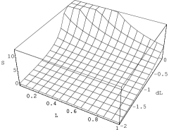
(b) Dependence on both variables.

Figure C.1: The bubble minus background action as a function of the cosmological constants. The variables are $S=\kappa_{4}^{4}T^{2}\Delta S$, $L=\Lambda_{-}/\kappa_{4}^{4}T^{2}$, and $dL=\Delta\Lambda/\kappa_{4}^{4}T^{2}$.

We should note that this action reduces to the known formulae in special cases. In particular, the result of CDL as quoted in [156],

$$\Delta S_{E}=-\frac{S_{0}}{\left(1+T_{c}^{2}/T^{2}\right)^{2}}$$ (C.11)

is valid for all tensions when the final vacuum energy vanishes. A related result is that, for any $\Lambda_{\pm}\geq 0$, as the bubble tension goes to infinity, the decay time goes to the recurrence time of the original dS.

As final comments, let us reemphasize, following [171, 173], that the final states are not maximally symmetric spacetimes but rather cosmological ones. In particular, decays with a negative final cosmological constant lead not to AdS but to a Big Crunch singularity within the bubble. Additionally, as mentioned in [173], these instantons are technically different from instanton decays of inflationary spacetimes. It seems reasonable that for sufficiently small decay rates that treating the initial spacetime as dS is a good approximation, but it remains an interesting problem to study decays of possibly more cosmologically relevant spacetimes.

C.3 Migration of D3-branes

The NS5-brane decay leaves D3-branes at the tip of the throat where it occurs. In this appendix we analyze their subsequent classical motion in configurations with multiple throats. The D3-branes, produced by a decay in one throat (Throat 1), are attracted by $\overline{\textnormal{D3}}$-branes in another throat (Throat 2), migrate across the compact manifold $M$, and eventually annihilate the $\overline{\textnormal{D3}}$-branes. As discussed in section 4.3.2, the decay times are so large that the migration times have little effect. We assume that the back-reaction of the migrating D3-branes is negligible, the proper velocity of the branes remains small, and that the majority of the travel time comes from the two throats (i.e. the time through the bulk of the CY may be ignored).

We ignore the most of the details coming from the deformation of the conifold since the motion is assumed to be radial. We will use the undeformed metric (2.39) and, when working near the tip, multiply the warp factor $e^{-4A}$ by an overall constant $\sim 0.4$ to account for the deformation. The warp factor, away from the tip, is

$$e^{-4A} = \frac{L^{4}}{r^{4}}\ln(r/r_{s})$$ (C.12)

$$r_{s} = r_{0}\ \exp(-\frac{2\pi(N+p)}{3g_{s}M^{2}}-\frac{1}{4})$$ (C.13)

$$p \equiv \#\textnormal{ of $\overline{\textnormal{D3}}$-branes}\ ;\ \ r_{0}^{2}=3/2^{5/3}\ \ .$$ (C.14)

Due to the deformation of the conifold discussed above we will only be interested in the region $\tilde{r}=r_{s}\exp(1/4)\leq r\leq r_{0}$. Note that this avoids the naked singularity at $r=r_{s}$.

The Ramond-Ramond potential $C_{4}$ depends only on the radial distance $r$:

$$C_{4}=\frac{f(r)}{g_{s}}dt\wedge dx^{1}\wedge dx^{2}\wedge dx^{3}$$ (C.15)

where $t\equiv x^{0}$. Working in the gauge $\xi^{0}=\tau(t)$ (proper time) and $\xi^{i}=x^{i}$, the D3-brane Lagrangian becomes,

$$\mu_{3}^{-1}\mathcal{L}=-\frac{e^{4A}}{g_{s}}(\sqrt{\dot{t}^{2}-e^{-4A}\dot{r}^{2}})+f(r)\dot{t}.$$ (C.16)

Assuming that the proper velocity is small,

$$\mu_{3}^{-1}\mathcal{L}\simeq\frac{1}{2}\frac{\dot{r}^{2}\dot{t}^{-1}}{g_{s}}-\frac{(e^{4A}-g_{s}f(r))}{g_{s}}\dot{t}$$ (C.17)

It is easy to check that this a valid approximation. In particular, one only needs to consider throat 2, since this is where the D3-branes are moving fastest. One can show that $p<<(g_{s}M^{2})/8$ will insure that (C.17) is valid.

Since $t(\tau)$ is a cyclic variable, we know that $\partial\mathcal{L}/\partial\dot{t}\equiv-E/g_{s}$ is constant, leaving us with

$$E=\frac{1}{2}(\partial_{t}r)^{2}+V(r)\ ;\ \ V(r)\equiv(e^{4A}-f(r))\ \ ,$$ (C.18)

and the travel time through a single throat is therefore,

$$\Delta t=\pm\int_{r_{0}}^{\tilde{r}}\frac{dr}{\sqrt{2(E-V(r))}}\ \ .$$ (C.19)

The $+/-$ corresponds to branes traveling into/out of the throat.

Note that the time here is a coordinate time, but we will see that it is so small compared to decay times that we do not need to worry about conversion to proper time in the 4D Einstein frame.

C.3.1 Throat 1

The D3-branes, produced at rest in throat 1, feel a slight gravitational attraction to the $\overline{\textnormal{D3}}$-branes at the bottom of throat 2. We see below that almost all the migration time does come in throat 1.

The Ramond-Ramond potential, $C_{4}=e^{4A_{1}}/g_{s}$, is not effected by charge contained in throat 2. Physically, this is due to the charge being screened; mathematically, we are working on a compact manifold and may consider just the charge enclosed in throat 1. However, the geometry does, albeit slightly, know about what is happening in throat 2.

In order to get an estimate of the migration time we will make the (perhaps bold) assumption that, as with most multi-pole solutions in gravity, the warp factor is changed by an additive factor,

$$e^{-4A_{1}}(r)\to e^{-4A_{1}}(r)+\delta(r);\ \ \delta(r)\equiv-\frac{27\pi\alpha^{\prime}}{(2r_{0}-r)^{4}}\left(N_{2}+p+3g_{s}M^{2}/8\pi\right)\ .$$ (C.20)

Here, the subscripts indicate the throat in which the fluxes are contained, $p$ is the number of $\overline{\textnormal{D3}}$-branes in throat 2 (there are no $\overline{\textnormal{D3}}$-branes in throat 1). Expanding to first order in $\delta$, we see that

$$V(r)=-\frac{27\pi\alpha^{\prime}}{(2r_{0}-r)^{4}}\left(N_{2}+p+3g_{s}M^{2}/8\pi\right)e^{8A_{1}}(r)\ \ .$$ (C.21)

(a) Throat 1

(b) Throat 2

Figure C.2: The potential for D3-branes in the presenece of $\overline{\textnormal{D3}}$-branes on the compact manifold.

Figure C.2(a) shows the this potential. Note that the majority of the time will be spent at the tip of this throat. We have been unable to evaluate the integral (C.19) explicitly. However, one may gain control of the situation by linearizing the potential near $r=\tilde{r}$ (where the branes are at rest) and integrate numerically. It is in this limit that we multiply $e^{-4A}$ by the numerical factor $\sim 0.4$ discussed above. Once a safe distance away from $r=\tilde{r}$, which for technical reasons coming from the linearization of (C.21) we take to be $r\sim\tilde{r}+zr_{0}$, one may evaluate the rest of the integral (C.19) numerically. For model 1, one finds that

$$\Delta t_{1}=1.5\times 10^{16}\ .$$ (C.22)

C.3.2 Throat 2

For completeness, we will determine time spent in throat 2, subsequently showing that it is of no importance. In order to deduce $C_{4}$, recall that $\int\star dC_{4}\sim(N_{\textnormal{eff}}-p)$. Plugging in the appropriate constants, this leaves us with

$$r^{5}e^{-8A}\partial_{r}f=(27\pi{\alpha^{\prime}}^{2})(N_{\textnormal{eff}}-p)\ \ .$$ (C.23)

Using what we know from the geometry, we define $f=e^{4A}+V$, where the potential, $V(r)$, satisfies

$$\partial_{r}V=\frac{(27\pi{\alpha^{\prime}}^{2}g_{s})p}{L^{5}}\frac{r^{3}/L^{3}}{(\ln(r/r_{s+}))}\ \ .$$ (C.24)

This can be integrated and gives a solution depending on exponential- integral functions. The potential is shown in figure C.2(b). Numerically integrating (C.19) for throat 2 gives

$$\Delta t_{2}\approx 9.9\ ,$$ (C.25)

which is clearly negligible compared to (C.22).

C.4 $\alpha^{\prime}$ Corrections in Asymmetric Warping

C.4.1 Calculation of Scalar MAVs

Here we demonstrate how to calculate the $\alpha^{\prime}$ corrections to the D3-brane scalar kinetic terms in the presence of the asymmetrically warped metric (5.2). We keep only the Lorentz violating terms.

We start by specifying the tangent to the D-brane, which we take as $\partial_{\alpha}X^{\mu}=\delta^{\mu}_{\alpha}$ with perturbatively small $\partial_{\alpha}X^{m}$. Then the normal bundle vielbein satisfies

$$\partial_{\alpha}X^{M}\xi^{\hat{a}}_{M}=0\ \mathnormal{or}\ \xi^{\hat{a}}_{\mu}=-\delta^{\alpha}_{\mu}\partial_{\alpha}X^{m}\xi^{\hat{a}}_{m}$$ (C.26)

which has solution to second order

$$\xi^{\hat{a}}_{\mu}=-\delta^{\alpha}_{\mu}\partial_{\alpha}X^{m}e_{m}^{\hat{m}}\delta^{\hat{a}}_{\hat{m}}\ ,\ \xi^{\hat{a}}_{m}=\delta^{\hat{a}}_{\hat{m}}e^{\hat{m}}_{m}-\frac{1}{2}g^{\mu\nu}\delta_{\mu}^{\alpha}\delta_{\nu}^{\beta}\partial_{\alpha}X^{p}\partial_{\beta}X^{n}\hat{e}_{n}^{\hat{n}}\delta_{\hat{n}}^{\hat{a}}g_{mp}\ .$$ (C.27)

Here $e^{\hat{m}}_{m}$ is the vielbein of $g_{mn}$ and is trivial at the position of the brane (we use Riemann normal coordinates on the compact manifold at the brane position). Since its expansion would just give powers of $X^{m}$ and not derivatives, we will ignore it from now on. Also, for notational convenience, since the normal bundle indices $\hat{a}$ always enter through Kronecker deltas with compact space indices, we will abuse notation slightly and replace $\hat{a}$ with $m$ in future formulae.

The nonvanishing Christoffel symbols are

$$\Gamma^{0}_{0m}=\partial_{m}A\ ,\ \Gamma^{m}_{00}=g^{mn}e^{A}\partial_{n}A\ ,\ \Gamma^{i}_{jm}=\partial_{m}B\delta^{i}_{j}\ ,\ \Gamma^{m}_{ij}=-g^{mn}e^{B}\partial_{n}B\delta_{ij}$$ (C.28)

on the spacetime and

$$(\Gamma_{T})^{0}_{00} = \partial_{0}X^{m}\partial_{m}A\ ,\ (\Gamma_{T})^{0}_{0i}=\partial_{i}X^{m}\partial_{m}A\ ,\ (\Gamma_{T})^{i}_{00}=e^{A-B}\delta^{ij}\partial_{j}X^{m}\partial_{m}A$$

$$(\Gamma_{T})^{0}_{ij} = e^{B-A}\delta_{ij}\partial_{0}X^{m}\partial_{m}B\ ,\ (\Gamma_{T})^{i}_{0j}=\delta^{i}_{j}\partial_{0}X^{m}\partial_{m}B$$

$$(\Gamma_{T})^{i}_{jk} = \left(\delta^{i}_{k}\partial_{j}X^{m}+\delta^{i}_{j}\partial_{k}X^{m}-\delta_{jk}\delta^{il}\partial_{l}X^{m}\right)\partial_{m}B$$ (C.29)

on the tangent space. This is just the Christoffel symbol of the pulled-back metric $g_{\alpha\beta}$. Plugging into eqn (B.7), we can very easily get eqn (5.4) for the extrinsic curvature.

Then, from eqn (B.8), the tangent Riemann components out to $\mathcal{O}(\partial X^{m})^{2}$ are

$$(R_{T})_{0i0j} = -a^{m}b_{m}\delta_{ij}+2a_{m}b_{n}\delta_{ij}\partial_{0}X^{m}\partial_{0}X^{n}-2a_{(m}b_{n)}\partial_{i}X^{m}\partial_{j}X^{n}$$

$$-\left(a_{mn}+3a_{m}a_{n}\right)\partial_{i}X^{m}\partial_{j}X^{n}+\left(b_{mn}+b_{m}b_{n}\right)\delta_{ij}\partial_{0}X^{m}\partial_{0}X^{n}$$

$$(R_{T})_{ijkl} = b^{2}\left(\delta_{ik}\delta_{jl}-\delta_{il}\delta_{jk}\right)+\left(b_{mn}+3b_{m}b_{n}\right)\left(\partial_{i}X^{m}\partial_{k}X^{n}\delta_{jl}\right.$$ (C.30)

$$\left.+\partial_{j}X^{m}\partial_{l}X^{n}\delta_{ik}-\partial_{i}X^{m}\partial_{l}X^{n}\delta_{jk}-\partial_{j}X^{m}\partial_{k}X^{n}\delta_{il}\right)\ .$$

The other components are only $\mathcal{O}(\partial X^{m})^{2}$, so they square to $\mathcal{O}(\partial X^{m})^{4}$. When squaring, we also need to take into account the second order part of the inverse metric pull-back. Note that the only terms involving $\Lambda$ come from $(R_{T})_{0i0j}$. To get $(R_{T})_{\alpha\beta}$ we just contract the Riemann tensor, being careful of second order terms in the metric.

From eqn (B.9), the normal bundle Riemann tensor is always second order in $\partial X^{m}$, so it does not contribute to the kinetic terms. That leaves just $\bar{R}^{mn}$. We end up with

$$\bar{R}^{mn} = -\left(a^{mn}+2a^{m}a^{n}\right)-3b^{mn}+R_{p}{}^{mn}{}_{q}\partial_{\mu}X^{p}\partial^{\mu}X^{q}$$ (C.31)

$$-2\left(a_{p}{}^{(m}+3a_{p}a^{(m}\right)\partial_{0}X^{n)}\partial_{0}X^{p}-\left(b_{p}{}^{(m}-3b_{p}b^{(m}\right)\vec{\partial}X^{m}\cdot\vec{\partial}X^{n}$$

$$-\left(a^{mn}+5a^{m}a^{n}\right)\delta_{pq}\partial_{0}X^{p}\partial_{0}X^{q}$$

$$+\left(b^{mn}-b^{m}b^{n}\right)\delta_{pq}\vec{\partial}X^{p}\cdot\vec{\partial}X^{q}\ .$$

Here $R_{mnpq}$ is the Riemann tensor of $g_{mn}$; note that it enters in a Lorentz invariant fashion. Getting the action (5.5) is just a matter of squaring.

C.4.2 T Duality for Photon MAV

Our T duality argument runs as follows. Suppose we compactify one of the noncompact spatial dimensions, say $x^{3}$, on a large circle. Then we perform T duality on $x^{3}$, giving a metric of

$$ds^{2}=-e^{2A}dt^{2}+e^{2B}\sum_{i=1}^{2}\left(dx^{i}\right)^{2}+e^{-2B}\left(dx^{3}\right)^{2}+g_{mn}dx^{m}dx^{n}$$ (C.32)

with, as before, all components of the metric depending only on $x^{m}$. Now $x^{3}$ is compactified on a small circle, and the braneworld is a D2-brane. In fact, this metric is of the same form as our original metric (5.2) except that $x^{3}$ is not a Riemann normal coordinate. The only difference this makes from the calculations of scalar calculation is that we now have to keep in mind that there is a nonvanishing Christoffel symbol $\Gamma^{m}_{33}$ that contributes kinetic terms to $\Omega^{m}_{\alpha\beta}$ ($\Gamma^{3}_{3m}$ will not matter because $\Omega^{3}_{\alpha\beta}$ will already be second order in $\partial X$). Otherwise some numerical factors differ. If we recalculate equation (5.5) for fluctuations of $X^{3}$ in 2 dimensions, we find

$$\delta S = \frac{\mu_{2}}{g_{s,2}}\int d^{3}x\frac{(2\pi\alpha^{\prime})^{2}}{192}\left|\vec{\partial}X^{3}\right|^{2}\left[44b^{2}b\cdot\lambda+12b^{mn}\lambda_{mn}+24\lambda^{mn}b_{m}b_{n}\right.$$ (C.33)

$$\left.+72b^{mn}\lambda_{m}b_{n}\right]\ .$$

Here $\mu_{2},g_{s,2}$ are the appropriate tension and string coupling for the D2-brane case.

If we then T-dualize back to the D3-brane and take the $x^{3}$ circle radius to infinity, we get back the original tension and string coupling and take $X^{3}\to(2\pi\alpha^{\prime})A_{3}$. Then by gauge invariance, we must replace $(2\pi\alpha^{\prime})\partial_{i}A_{3}\to\mathcal{F}_{i3}$, and isotropy requires that we promote $\mathcal{F}_{i3}\mathcal{F}^{i3}\to\mathcal{F}_{ij}\mathcal{F}^{ij}$. Then we get the result (5.6).

Bibliography

- [1] A. R. Frey and J. Polchinski, “N = 3 warped compactifications,” Phys. Rev. D65 (2002) 126009, hep-th/0201029.
- [2] M. Graña and A. R. Frey, “BPS states of strings in 3-form flux,” Phys. Rev. D67 (2003) 026008, hep-th/0208032.
- [3] A. R. Frey and A. Mazumdar, “3-form induced potentials, dilaton stabilization, and running moduli,” Phys. Rev. D67 (2003) 046006, hep-th/0210254.
- [4] A. R. Frey, “String theoretic bounds on Lorentz-violating warped compactification,” JHEP 04 (2003) 012, hep-th/0301189.
- [5] A. R. Frey, M. Lippert, and B. Williams, “The Fall of Stringy de Sitter,” hep-th/0305018.
- [6] A. R. Frey and M. Graña, “Type IIB solutions with interpolating supersymmetries,” hep-th/0307142.
- [7] N. Arkani-Hamed, S. Dimopoulos, and G. R. Dvali, “The hierarchy problem and new dimensions at a millimeter,” Phys. Lett. B429 (1998) 263–272, hep-ph/9803315.
- [8] V. A. Rubakov and M. E. Shaposhnikov, “Do we live inside a domain wall?,” Phys. Lett. B125 (1983) 136–138.
- [9] K. Akama, “An early proposal of ’brane world’,” Lect. Notes Phys. 176 (1982) 267–271, hep-th/0001113.
- [10] I. Antoniadis, N. Arkani-Hamed, S. Dimopoulos, and G. R. Dvali, “New dimensions at a millimeter to a Fermi and superstrings at a TeV,” Phys. Lett. B436 (1998) 257–263, hep-ph/9804398.
- [11] L. Randall and R. Sundrum, “A large mass hierarchy from a small extra dimension,” Phys. Rev. Lett. 83 (1999) 3370–3373, hep-ph/9905221.
- [12] L. Randall and R. Sundrum, “An alternative to compactification,” Phys. Rev. Lett. 83 (1999) 4690–4693, hep-th/9906064.
- [13] H. Verlinde, “Holography and compactification,” Nucl. Phys. B580 (2000) 264–274, hep-th/9906182.
- [14] C. S. Chan, P. L. Paul, and H. Verlinde, “A note on warped string compactification,” Nucl. Phys. B581 (2000) 156–164, hep-th/0003236.
- [15] C. Csaki, J. Erlich, T. J. Hollowood, and Y. Shirman, “Universal aspects of gravity localized on thick branes,” Nucl. Phys. B581 (2000) 309–338, hep-th/0001033.
- [16] B. R. Greene, K. Schalm, and G. Shiu, “Warped compactifications in M and F theory,” Nucl. Phys. B584 (2000) 480–508, hep-th/0004103.
- [17] J. Polchinski, “String theory. Vol. 2: Superstring theory and beyond,”. Cambridge, UK: Univ. Pr. (1998) 531 p.
- [18] O. DeWolfe and S. B. Giddings, “Scales and hierarchies in warped compactifications and brane worlds,” hep-th/0208123.
- [19] W. D. Goldberger and M. B. Wise, “Modulus stabilization with bulk fields,” Phys. Rev. Lett. 83 (1999) 4922–4925, hep-ph/9907447.
- [20] W. D. Goldberger and M. B. Wise, “Phenomenology of a stabilized modulus,” Phys. Lett. B475 (2000) 275–279, hep-ph/9911457.
- [21] P. Mayr, “Stringy world branes and exponential hierarchies,” JHEP 11 (2000) 013, hep-th/0006204.
- [22] K. Becker and M. Becker, “M-Theory on Eight-Manifolds,” Nucl. Phys. B477 (1996) 155–167, hep-th/9605053.
- [23] K. Dasgupta, G. Rajesh, and S. Sethi, “M theory, orientifolds and G-flux,” JHEP 08 (1999) 023, hep-th/9908088.
- [24] S. B. Giddings, S. Kachru, and J. Polchinski, “Hierarchies from fluxes in string compactifications,” Phys. Rev. D66 (2002) 106006, hep-th/0105097.
- [25] J. Polchinski and A. Strominger, “New Vacua for Type II String Theory,” Phys. Lett. B388 (1996) 736–742, hep-th/9510227.
- [26] J. Michelson, “Compactifications of type IIB strings to four dimensions with non-trivial classical potential,” Nucl. Phys. B495 (1997) 127–148, hep-th/9610151.
- [27] T. R. Taylor and C. Vafa, “RR flux on Calabi-Yau and partial supersymmetry breaking,” Phys. Lett. B474 (2000) 130–137, hep-th/9912152.
- [28] G. Curio, A. Klemm, D. Lust, and S. Theisen, “On the vacuum structure of type II string compactifications on Calabi-Yau spaces with H-fluxes,” Nucl. Phys. B609 (2001) 3–45, hep-th/0012213.
- [29] G. Curio, A. Klemm, B. Kors, and D. Lust, “Fluxes in heterotic and type II string compactifications,” Nucl. Phys. B620 (2002) 237–258, hep-th/0106155.
- [30] G. Dall’Agata, “Type IIB supergravity compactified on a Calabi-Yau manifold with H-fluxes,” JHEP 11 (2001) 005, hep-th/0107264.
- [31] B. de Wit, D. J. Smit, and N. D. Hari Dass, “Residual supersymmetry of compactified d = 10 supergravity,” Nucl. Phys. B283 (1987) 165.
- [32] J. M. Maldacena and C. Nuñez, “Supergravity description of field theories on curved manifolds and a no go theorem,” Int. J. Mod. Phys. A16 (2001) 822–855, hep-th/0007018.
- [33] A. Sen, “F-theory and Orientifolds,” Nucl. Phys. B475 (1996) 562–578, hep-th/9605150.
- [34] S. Sethi, C. Vafa, and E. Witten, “Constraints on low-dimensional string compactifications,” Nucl. Phys. B480 (1996) 213–224, hep-th/9606122.
- [35] A. Dabholkar and J. Park, “Strings on Orientifolds,” Nucl. Phys. B477 (1996) 701–714, hep-th/9604178.
- [36] P. K. Tripathy and S. P. Trivedi, “Compactification with flux on K3 and tori,” JHEP 03 (2003) 028, hep-th/0301139.
- [37] K. Becker and K. Dasgupta, “Heterotic strings with torsion,” hep-th/0209077.
- [38] E. Witten, “Baryons and branes in anti de Sitter space,” JHEP 07 (1998) 006, hep-th/9805112.
- [39] A. Hanany and B. Kol, “On orientifolds, discrete torsion, branes and M theory,” JHEP 06 (2000) 013, hep-th/0003025.
- [40] O. Bergman, E. G. Gimon, and S. Sugimoto, “Orientifolds, RR torsion, and K-theory,” JHEP 05 (2001) 047, hep-th/0103183.
- [41] E. Witten, “Toroidal compactification without vector structure,” JHEP 02 (1998) 006, hep-th/9712028.
- [42] D. Martelli and J. Sparks, “G-structures, fluxes and calibrations in M-theory,” hep-th/0306225.
- [43] A. Strominger, “Superstrings with torsion,” Nucl. Phys. B274 (1986) 253.
- [44] J. M. Maldacena and C. Nuñez, “Towards the large N limit of pure N = 1 super Yang Mills,” Phys. Rev. Lett. 86 (2001) 588–591, hep-th/0008001.
- [45] K. Becker, M. Becker, K. Dasgupta, and P. S. Green, “Compactifications of heterotic theory on non-Kaehler complex manifolds. I,” JHEP 04 (2003) 007, hep-th/0301161.
- [46] M. Graña and J. Polchinski, “Supersymmetric three-form flux perturbations on AdS(5),” Phys. Rev. D63 (2001) 026001, hep-th/0009211.
- [47] S. S. Gubser, “Supersymmetry and F-theory realization of the deformed conifold with three-form flux,” hep-th/0010010.
- [48] A. Kehagias, “New type IIB vacua and their F-theory interpretation,” Phys. Lett. B435 (1998) 337–342, hep-th/9805131.
- [49] M. Graña and J. Polchinski, “Gauge / gravity duals with holomorphic dilaton,” Phys. Rev. D65 (2002) 126005, hep-th/0106014.
- [50] J. H. Schwarz and P. C. West, “Symmetries and transformations of chiral N=2 D = 10 supergravity,” Phys. Lett. B126 (1983) 301.
- [51] J. H. Schwarz, “Covariant field equations of chiral N=2 D = 10 supergravity,” Nucl. Phys. B226 (1983) 269.
- [52] E. Bergshoeff, M. de Roo, B. Janssen, and T. Ortin, “The super D9-brane and its truncations,” Nucl. Phys. B550 (1999) 289–302, hep-th/9901055.
- [53] S. F. Hassan, “T-duality, space-time spinors and R-R fields in curved backgrounds,” Nucl. Phys. B568 (2000) 145–161, hep-th/9907152.
- [54] A. Buchel and A. R. Frey, “Comments on supergravity dual of pure N = 1 super Yang Mills theory with unbroken chiral symmetry,” Phys. Rev. D64 (2001) 064007, hep-th/0103022.
- [55] J. Scherk and J. H. Schwarz, “How to get masses from extra dimensions,” Nucl. Phys. B153 (1979) 61–88.
- [56] S. P. de Alwis, “On potentials from fluxes,” hep-th/0307084.
- [57] S. B. Giddings and A. Maharana. work in progress.
- [58] S. Gukov, C. Vafa, and E. Witten, “CFT’s from Calabi-Yau four-folds,” Nucl. Phys. B584 (2000) 69–108, hep-th/9906070.
- [59] S. Gukov, “Solitons, superpotentials and calibrations,” Nucl. Phys. B574 (2000) 169–188, hep-th/9911011.
- [60] S. Kachru, X. Liu, M. B. Schulz, and S. P. Trivedi, “Supersymmetry changing bubbles in string theory,” hep-th/0205108.
- [61] P. Candelas and X. de la Ossa, “Moduli space of Calabi-Yau manifolds,” Nucl. Phys. B355 (1991) 455–481.
- [62] S. Kachru et al., “Towards inflation in string theory,” hep-th/0308055.
- [63] E. Cremmer, S. Ferrara, C. Kounnas, and D. V. Nanopoulos, “Naturally vanishing cosmological constant in N=1 supergravity,” Phys. Lett. B133 (1983) 61.
- [64] J. R. Ellis, A. B. Lahanas, D. V. Nanopoulos, and K. Tamvakis, “No - scale supersymmetric standard model,” Phys. Lett. B134 (1984) 429.
- [65] E. Witten, “Dimensional reduction of superstring models,” Phys. Lett. B155 (1985) 151.
- [66] M. Dine, R. Rohm, N. Seiberg, and E. Witten, “Gluino condensation in superstring models,” Phys. Lett. B156 (1985) 55.
- [67] I. R. Klebanov and M. J. Strassler, “Supergravity and a confining gauge theory: Duality cascades and chiSB-resolution of naked singularities,” JHEP 08 (2000) 052, hep-th/0007191.
- [68] P. Candelas and X. C. de la Ossa, “Comments on conifolds,” Nucl. Phys. B342 (1990) 246–268.
- [69] C. P. Herzog, I. R. Klebanov, and P. Ouyang, “Remarks on the warped deformed conifold,” hep-th/0108101.
- [70] I. R. Klebanov and A. A. Tseytlin, “Gravity duals of supersymmetric SU(N) x SU(N+M) gauge theories,” Nucl. Phys. B578 (2000) 123–138, hep-th/0002159.
- [71] A. Strominger, “Massless black holes and conifolds in string theory,” Nucl. Phys. B451 (1995) 96–108, hep-th/9504090.
- [72] S. Kachru, M. Schulz, and S. Trivedi, “Moduli stabilization from fluxes in a simple IIB orientifold,” hep-th/0201028.
- [73] S. Kachru, M. B. Schulz, P. K. Tripathy, and S. P. Trivedi, “New supersymmetric string compactifications,” JHEP 03 (2003) 061, hep-th/0211182.
- [74] S. Ferrara and C. Kounnas, “Extended supersymmetry in four-dimensional type II strings,” Nucl. Phys. B328 (1989) 406.
- [75] L. Castellani, A. Ceresole, S. Ferrara, R. D’Auria, P. Fre, and E. Maina, “The complete N=3 matter coupled supergravity,” Nucl. Phys. B268 (1986) 317.
- [76] V. A. Tsokur and Y. M. Zinoviev, “Spontaneous supersymmetry breaking in N = 4 supergravity with matter,” Phys. Atom. Nucl. 59 (1996) 2192–2197, hep-th/9411104.
- [77] L. Andrianopoli, R. D’Auria, S. Ferrara, and M. A. Lledo, “Gauging of flat groups in four dimensional supergravity,” hep-th/0203206.
- [78] L. Andrianopoli, R. D’Auria, S. Ferrara, and M. A. Lledo, “Duality and spontaneously broken supergravity in flat backgrounds,” hep-th/0204145.
- [79] R. D’Auria, S. Ferrara, and S. Vaula, “N = 4 gauged supergravity and a IIB orientifold with fluxes,” hep-th/0206241.
- [80] S. Ferrara and M. Porrati, “N = 1 no-scale supergravity from IIB orientifolds,” hep-th/0207135.
- [81] R. D’Auria, S. Ferrara, M. A. Lledo, and S. Vaula, “No-scale N = 4 supergravity coupled to Yang-Mills: The scalar potential and super Higgs effect,” Phys. Lett. B557 (2003) 278–282, hep-th/0211027.
- [82] L. Andrianopoli, R. D’Auria, S. Ferrara, and M. A. Lledo, “Gauged extended supergravity without cosmological constant: No-scale structure and supersymmetry breaking,” hep-th/0212141.
- [83] L. Andrianopoli, R. D’Auria, S. Ferrara, and M. A. Lledo, “N = 2 super-Higgs, N = 1 Poincare vacua and quaternionic geometry,” JHEP 01 (2003) 045, hep-th/0212236.
- [84] L. Andrianopoli, R. D’Auria, S. Ferrara, and M. A. Lledo, “4-D gauged supergravity analysis of type IIB vacua on K3 x T**2/Z(2),” JHEP 03 (2003) 044, hep-th/0302174.
- [85] L. Andrianopoli, S. Ferrara, and M. Trigiante, “Fluxes, supersymmetry breaking and gauged supergravity,” hep-th/0307139.
- [86] R. D’Auria, S. Ferrara, F. Gargiulo, M. Trigiante, and S. Vaula, “N = 4 supergravity Lagrangian for type IIB on T**6/Z(2) in presence of fluxes and D3-branes,” hep-th/0303049.
- [87] C. Angelantonj, S. Ferrara, and M. Trigiante, “New D = 4 gauged supergravities from N = 4 orientifolds with fluxes,” hep-th/0306185.
- [88] S. Ferrara, “Duality, gauging and superHiggs effect in string and M- theory,” hep-th/0211116.
- [89] M. de Roo and P. Wagemans, “Partial supersymmetry breaking in N=4 supergravity,” Phys. Lett. B177 (1986) 352.
- [90] P. Wagemans, “Breaking of N=4 supergravity to N=1, N=2 at lambda = 0,” Phys. Lett. B206 (1988) 241.
- [91] L. Andrianopoli, R. D’Auria, and S. Ferrara, “Supersymmetry reduction of N-extended supergravities in four dimensions,” JHEP 03 (2002) 025, hep-th/0110277.
- [92] L. Andrianopoli, R. D’Auria, S. Ferrara, and M. A. Lledo, “Super Higgs effect in extended supergravity,” hep-th/0202116.
- [93] M. K. Gaillard and B. Zumino, “Duality rotations for interacting fields,” Nucl. Phys. B193 (1981) 221.
- [94] R. C. Myers, “Dielectric-branes,” JHEP 12 (1999) 022, hep-th/9910053.
- [95] K. S. Narain, “New heterotic string theories in uncompactified dimensions ¡ 10,” Phys. Lett. B169 (1986) 41.
- [96] K. S. Narain, M. H. Sarmadi, and E. Witten, “A note on toroidal compactification of heterotic string theory,” Nucl. Phys. B279 (1987) 369.
- [97] S. Ferrara, C. Kounnas, and M. Porrati, “General dimensional reduction of ten-dimensional supergravity and superstring,” Phys. Lett. B181 (1986) 263.
- [98] B. A. Ovrut, “Moduli, matter scalars and the effective Lagrangian of superstrings,” Nucl. Phys. Proc. Suppl. 11 (1989) 378–388.
- [99] J. Maharana and J. H. Schwarz, “Noncompact symmetries in string theory,” Nucl. Phys. B390 (1993) 3–32, hep-th/9207016.
- [100] E. G. Gimon and J. Polchinski, “Consistency Conditions for Orientifolds and D-Manifolds,” Phys. Rev. D54 (1996) 1667–1676, hep-th/9601038.
- [101] A. Sen, “Strong - weak coupling duality in four-dimensional string theory,” Int. J. Mod. Phys. A9 (1994) 3707–3750, hep-th/9402002.
- [102] J. H. Schwarz and A. Sen, “Duality symmetries of 4-D heterotic strings,” Phys. Lett. B312 (1993) 105–114, hep-th/9305185.
- [103] E. Witten, “Small Instantons in String Theory,” Nucl. Phys. B460 (1996) 541–559, hep-th/9511030.
- [104] C. Kounnas and A. Kumar, “BPS states in N = 3 superstrings,” Nucl. Phys. B511 (1998) 216–242, hep-th/9709061.
- [105] O. Aharony and A. Hanany, “Branes, superpotentials and superconformal fixed points,” Nucl. Phys. B504 (1997) 239–271, hep-th/9704170.
- [106] O. Aharony, A. Hanany, and B. Kol, “Webs of (p,q) 5-branes, five dimensional field theories and grid diagrams,” JHEP 01 (1998) 002, hep-th/9710116.
- [107] K. Becker, M. Becker, and A. Strominger, “Five-branes, membranes and nonperturbative string theory,” Nucl. Phys. B456 (1995) 130–152, hep-th/9507158.
- [108] E. Witten, “Non-Perturbative Superpotentials In String Theory,” Nucl. Phys. B474 (1996) 343–360, hep-th/9604030.
- [109] J. A. Harvey and G. W. Moore, “Superpotentials and membrane instantons,” hep-th/9907026.
- [110] E. Witten, “World-sheet corrections via D-instantons,” JHEP 02 (2000) 030, hep-th/9907041.
- [111] E. H. Fradkin, “Field theories of condensed matter systems,”. Redwood City, USA: Addison-Wesley (1991) 350 p. (Frontiers in physics, 82).
- [112] E. Witten, “Constraints on supersymmetry breaking,” Nucl. Phys. B202 (1982) 253.
- [113] R. Casalbuoni, “The classical mechanics for Bose-Fermi systems,” Nuovo Cim. A33 (1976) 389.
- [114] J. Polchinski, “String theory. Vol. 1: An introduction to the bosonic string,”. Cambridge, UK: Univ. Pr. (1998) 402 p.
- [115] M. Cederwall, A. von Gussich, B. E. W. Nilsson, P. Sundell, and A. Westerberg, “The Dirichlet super-p-branes in ten-dimensional type IIA and IIB supergravity,” Nucl. Phys. B490 (1997) 179–201, hep-th/9611159.
- [116] E. Bergshoeff and P. K. Townsend, “Super D-branes,” Nucl. Phys. B490 (1997) 145–162, hep-th/9611173.
- [117] B. de Wit, K. Peeters, and J. Plefka, “Superspace geometry for supermembrane backgrounds,” Nucl. Phys. B532 (1998) 99–123, hep-th/9803209.
- [118] K. Millar, W. Taylor, and M. Van Raamsdonk, “D-particle polarizations with multipole moments of higher- dimensional branes,” hep-th/0007157.
- [119] M. Graña, “D3-brane action in a supergravity background: The fermionic story,” hep-th/0202118.
- [120] E. Bergshoeff, R. Kallosh, T. Ortin, and G. Papadopoulos, “Kappa-symmetry, supersymmetry and intersecting branes,” Nucl. Phys. B502 (1997) 149–169, hep-th/9705040.
- [121] R. Kallosh, “Worldvolume supersymmetry,” Phys. Rev. D57 (1998) 3214–3218, hep-th/9709069.
- [122] A. Keurentjes and S. Sethi, “Twisting E8 five-branes,” Phys. Rev. D66 (2002) 046001, hep-th/0205162.
- [123] M. Porrati, “How to find H-monopoles in brane dynamics,” Phys. Lett. B387 (1996) 492–496, hep-th/9607082.
- [124] S. Sethi and M. Stern, “A comment on the spectrum of H-monopoles,” Phys. Lett. B398 (1997) 47–51, hep-th/9607145.
- [125] K. Becker and M. Becker, “Supersymmetry breaking, M-theory and fluxes,” JHEP 07 (2001) 038, hep-th/0107044.
- [126] R. Argurio, V. L. Campos, G. Ferretti, and R. Heise, “Freezing of moduli with fluxes in three dimensions,” hep-th/0205295.
- [127] K. Becker, “A note on compactifications on Spin(7)-holonomy manifolds,” JHEP 05 (2001) 003, hep-th/0011114.
- [128] M. Berg, M. Haack, and H. Samtleben, “Calabi-Yau fourfolds with flux and supersymmetry breaking,” JHEP 04 (2003) 046, hep-th/0212255.
- [129] E. Bergshoeff, C. M. Hull, and T. Ortin, “Duality in the type II superstring effective action,” Nucl. Phys. B451 (1995) 547–578, hep-th/9504081.
- [130] A. Dabholkar and C. Hull, “Duality twists, orbifolds, and fluxes,” hep-th/0210209.
- [131] K. Becker and M. Becker, “Compactifying M-theory to four dimensions,” JHEP 11 (2000) 029, hep-th/0010282.
- [132] S. Gurrieri, J. Louis, A. Micu, and D. Waldram, “Mirror symmetry in generalized Calabi-Yau compactifications,” Nucl. Phys. B654 (2003) 61–113, hep-th/0211102.
- [133] C. L. Bennett et al., “First Year Wilkinson Microwave Anisotropy Probe (WMAP) Observations: Preliminary Maps and Basic Results,” astro-ph/0302207.
- [134] P. Fre, M. Trigiante, and A. Van Proeyen, “Stable de Sitter vacua from N = 2 supergravity,” Class. Quant. Grav. 19 (2002) 4167–4194, hep-th/0205119.
- [135] R. Kallosh, “Supergravity, M theory and cosmology,” hep-th/0205315.
- [136] R. Kallosh, A. Linde, S. Prokushkin, and M. Shmakova, “Supergravity, dark energy and the fate of the universe,” hep-th/0208156.
- [137] J. Polchinski and M. J. Strassler, “The string dual of a confining four-dimensional gauge theory,” hep-th/0003136.
- [138] D. Z. Freedman and J. A. Minahan, “Finite temperature effects in the supergravity dual of the N = 1* gauge theory,” JHEP 01 (2001) 036, hep-th/0007250.
- [139] A. R. Liddle, A. Mazumdar, and F. E. Schunck, “Assisted inflation,” Phys. Rev. D58 (1998) 061301, astro-ph/9804177.
- [140] E. J. Copeland, A. Mazumdar, and N. J. Nunes, “Generalized assisted inflation,” Phys. Rev. D60 (1999) 083506, astro-ph/9904309.
- [141] A. L. Berkin, K.-i. Maeda, and J. Yokoyama, “Soft inflation,” Phys. Rev. Lett. 65 (1990) 141–144.
- [142] A. L. Berkin and K.-I. Maeda, “Inflation in generalized Einstein theories,” Phys. Rev. D44 (1991) 1691–1704.
- [143] A. Mazumdar, “Extra dimensions and inflation,” Phys. Lett. B469 (1999) 55–60, hep-ph/9902381.
- [144] S. Hellerman, N. Kaloper, and L. Susskind, “String theory and quintessence,” JHEP 06 (2001) 003, hep-th/0104180.
- [145] W. Fischler, A. Kashani-Poor, R. McNees, and S. Paban, “The acceleration of the universe, a challenge for string theory,” JHEP 07 (2001) 003, hep-th/0104181.
- [146] S. B. Giddings, “The fate of four dimensions,” hep-th/0303031.
- [147] C. Kounnas and M. Quiros, “A maximally symmetric no scale inflationary universe,” Phys. Lett. B151 (1985) 189.
- [148] J. M. Molera and M. Quiros, “Analysis of no scale supergravity models leading to inflationary scenarios,” Phys. Rev. D36 (1987) 375–385.
- [149] R. Kallosh, A. D. Linde, S. Prokushkin, and M. Shmakova, “Gauged supergravities, de Sitter space and cosmology,” Phys. Rev. D65 (2002) 105016, hep-th/0110089.
- [150] F. Quevedo, “Lectures on string / brane cosmology,” Class. Quant. Grav. 19 (2002) 5721–5779, hep-th/0210292.
- [151] S. Kachru and L. McAllister, “Bouncing brane cosmologies from warped string compactifications,” JHEP 03 (2003) 018, hep-th/0205209.
- [152] A. Kehagias and E. Kiritsis, “Mirage cosmology,” JHEP 11 (1999) 022, hep-th/9910174.
- [153] K. Dasgupta, C. Herdeiro, S. Hirano, and R. Kallosh, “D3/D7 inflationary model and M-theory,” Phys. Rev. D65 (2002) 126002, hep-th/0203019.
- [154] R. Kallosh, “N = 2 supersymmetry and de Sitter space,” hep-th/0109168.
- [155] C. Herdeiro, S. Hirano, and R. Kallosh, “String theory and hybrid inflation / acceleration,” JHEP 12 (2001) 027, hep-th/0110271.
- [156] S. Kachru, R. Kallosh, A. Linde, and S. P. Trivedi, “De Sitter vacua in string theory,” hep-th/0301240.
- [157] E. Silverstein, “(A)dS backgrounds from asymmetric orientifolds,” hep-th/0106209.
- [158] P. Berglund, T. Hubsch, and D. Minic, “de Sitter spacetimes from warped compactifications of IIB string theory,” Phys. Lett. B534 (2002) 147–154, hep-th/0112079.
- [159] A. Klemm, B. Lian, S. S. Roan, and S. T. Yau, “Calabi-Yau fourfolds for M- and F-theory compactifications,” Nucl. Phys. B518 (1998) 515–574, hep-th/9701023.
- [160] P. Mayr, “On supersymmetry breaking in string theory and its realization in brane worlds,” Nucl. Phys. B593 (2001) 99–126, hep-th/0003198.
- [161] C. Escoda, M. Gomez-Reino, and F. Quevedo, “Saltatory de Sitter string vacua,” hep-th/0307160.
- [162] S. Kachru, J. Pearson, and H. Verlinde, “Brane/flux annihilation and the string dual of a non- supersymmetric field theory,” JHEP 06 (2002) 021, hep-th/0112197.
- [163] R. Bousso and J. Polchinski, “Quantization of four-form fluxes and dynamical neutralization of the cosmological constant,” JHEP 06 (2000) 006, hep-th/0004134.
- [164] M. R. Douglas, “The statistics of string / M theory vacua,” JHEP 05 (2003) 046, hep-th/0303194.
- [165] S. Ashok and M. R. Douglas, “Counting flux vacua,” hep-th/0307049.
- [166] B. R. Greene, “String theory on Calabi-Yau manifolds,” hep-th/9702155.
- [167] L. Dyson, M. Kleban, and L. Susskind, “Disturbing implications of a cosmological constant,” JHEP 10 (2002) 011, hep-th/0208013.
- [168] T. Banks, W. Fischler, and S. Paban, “Recurrent nightmares?: Measurement theory in de Sitter space,” JHEP 12 (2002) 062, hep-th/0210160.
- [169] N. Goheer, M. Kleban, and L. Susskind, “The trouble with de Sitter space,” hep-th/0212209.
- [170] M. Dine and N. Seiberg, “Is the superstring weakly coupled?,” Phys. Lett. B162 (1985) 299.
- [171] S. R. Coleman and F. De Luccia, “Gravitational effects on and of vacuum decay,” Phys. Rev. D21 (1980) 3305.
- [172] L. Susskind, “The anthropic landscape of string theory,” hep-th/0302219.
- [173] T. Banks, “Heretics of the false vacuum: Gravitational effects on and of vacuum decay. II,” hep-th/0211160.
- [174] J. D. Brown and C. Teitelboim, “Dynamical neutralization of the cosmological constant,” Phys. Lett. B195 (1987) 177–182.
- [175] J. D. Brown and C. Teitelboim, “Neutralization of the cosmological constant by membrane creation,” Nucl. Phys. B297 (1988) 787–836.
- [176] S. W. Hawking and I. G. Moss, “Supercooled phase transitions in the very early universe,” Phys. Lett. B110 (1982) 35.
- [177] J. L. Feng, J. March-Russell, S. Sethi, and F. Wilczek, “Saltatory relaxation of the cosmological constant,” Nucl. Phys. B602 (2001) 307–328, hep-th/0005276.
- [178] A. Maloney, E. Silverstein, and A. Strominger, “De Sitter space in noncritical string theory,” hep-th/0205316.
- [179] S. Weinberg, “Does gravitation resolve the ambiguity among supersymmetry vacua?,” Phys. Rev. Lett. 48 (1982) 1776–1779.
- [180] O. J. Ganor, “A note on zeroes of superpotentials in F-theory,” Nucl. Phys. B499 (1997) 55–66, hep-th/9612077.
- [181] S. R. Coleman, “The uses of instantons,”. Lecture delivered at 1977 Int. School of Subnuclear Physics, Erice, Italy, Jul 23-Aug 10, 1977.
- [182] A. Linde, “Fast-roll inflation,” JHEP 11 (2001) 052, hep-th/0110195.
- [183] G. N. Felder, A. V. Frolov, L. Kofman, and A. V. Linde, “Cosmology with negative potentials,” Phys. Rev. D66 (2002) 023507, hep-th/0202017.
- [184] R. Kallosh and A. Linde, “Dark energy and the fate of the universe,” JCAP 0302 (2003) 002, astro-ph/0301087.
- [185] M. Fabinger and E. Silverstein, “D-Sitter Space: Causal Structure, Thermodynamics, and Entropy,” hep-th/0304220.
- [186] S. Dimopoulos, S. Kachru, N. Kaloper, A. E. Lawrence, and E. Silverstein, “Generating small numbers by tunneling in multi-throat compactifications,” hep-th/0106128.
- [187] S. Dimopoulos, S. Kachru, N. Kaloper, A. E. Lawrence, and E. Silverstein, “Small numbers from tunneling between brane throats,” Phys. Rev. D64 (2001) 121702, hep-th/0104239.
- [188] B. S. Acharya, “M theory, Joyce orbifolds and super Yang-Mills,” Adv. Theor. Math. Phys. 3 (1999) 227–248, hep-th/9812205.
- [189] B. S. Acharya, “On realising N = 1 super Yang-Mills in M theory,” hep-th/0011089.
- [190] M. Atiyah and E. Witten, “M-theory dynamics on a manifold of G(2) holonomy,” Adv. Theor. Math. Phys. 6 (2003) 1–106, hep-th/0107177.
- [191] B. S. Acharya, “M theory, G(2)-manifolds and four-dimensional physics,” Class. Quant. Grav. 19 (2002) 5619–5653.
- [192] B. S. Acharya and B. Spence, “Flux, supersymmetry and M theory on 7-manifolds,” hep-th/0007213.
- [193] C. Beasley and E. Witten, “A note on fluxes and superpotentials in M-theory compactifications on manifolds of G(2) holonomy,” JHEP 07 (2002) 046, hep-th/0203061.
- [194] B. S. Acharya, “A moduli fixing mechanism in M theory,” hep-th/0212294.
- [195] G. L. Cardoso et al., “Non-Kaehler string backgrounds and their five torsion classes,” Nucl. Phys. B652 (2003) 5–34, hep-th/0211118.
- [196] J. P. Gauntlett, D. Martelli, and D. Waldram, “Superstrings with intrinsic torsion,” hep-th/0302158.
- [197] K. Becker, M. Becker, K. Dasgupta, and S. Prokushkin, “Properties of heterotic vacua from superpotentials,” hep-th/0304001.
- [198] G. L. Cardoso, G. Curio, G. Dall’Agata, and D. Lust, “BPS action and superpotential for heterotic string compactifications with fluxes,” hep-th/0306088.
- [199] M. Becker and D. Constantin, “A note on flux induced superpotentials in string theory,” hep-th/0210131.
- [200] S. Hellerman, J. McGreevy, and B. Williams, “Geometric constructions of nongeometric string theories,” hep-th/0208174.
- [201] K. S. Narain, M. H. Sarmadi, and C. Vafa, “Asymmetric orbifolds,” Nucl. Phys. B288 (1987) 551.
- [202] A. Sen and C. Vafa, “Dual pairs of type II string compactification,” Nucl. Phys. B455 (1995) 165–187, hep-th/9508064.
- [203] D. Berenstein, V. Jejjala, and R. G. Leigh, “The standard model on a D-brane,” Phys. Rev. Lett. 88 (2002) 071602, hep-ph/0105042.
- [204] J. F. G. Cascales and A. M. Uranga, “Chiral 4d N = 1 string vacua with D-branes and NSNS and RR fluxes,” JHEP 05 (2003) 011, hep-th/0303024.
- [205] R. Blumenhagen, D. Lust, and T. R. Taylor, “Moduli stabilization in chiral type IIB orientifold models with fluxes,” Nucl. Phys. B663 (2003) 319–342, hep-th/0303016.
- [206] K. Becker, M. Becker, M. Haack, and J. Louis, “Supersymmetry breaking and alpha’ corrections to flux induced potentials,” hep-th/0204254.
- [207] M. Graña, “MSSM parameters from supergravity backgrounds,” Phys. Rev. D67 (2003) 066006, hep-th/0209200.
- [208] S. Weinberg, “The cosmological constant problem,” Rev. Mod. Phys. 61 (1989) 1–23.
- [209] N. Arkani-Hamed, S. Dimopoulos, N. Kaloper, and R. Sundrum, “A small cosmological constant from a large extra dimension,” Phys. Lett. B480 (2000) 193–199, hep-th/0001197.
- [210] S. Kachru, M. B. Schulz, and E. Silverstein, “Self-tuning flat domain walls in 5d gravity and string theory,” Phys. Rev. D62 (2000) 045021, hep-th/0001206.
- [211] C. Csaki, J. Erlich, C. Grojean, and T. J. Hollowood, “General properties of the self-tuning domain wall approach to the cosmological constant problem,” Nucl. Phys. B584 (2000) 359–386, hep-th/0004133.
- [212] P. Kraus, “Dynamics of anti-de Sitter domain walls,” JHEP 12 (1999) 011, hep-th/9910149.
- [213] C. Csaki, J. Erlich, and C. Grojean, “Gravitational Lorentz violations and adjustment of the cosmological constant in asymmetrically warped spacetimes,” Nucl. Phys. B604 (2001) 312–342, hep-th/0012143.
- [214] C. Csaki, J. Erlich, and C. Grojean, “The cosmological constant problem in brane-worlds and gravitational Lorentz violations,” Gen. Rel. Grav. 33 (2001) 1921–1928, gr-qc/0105114.
- [215] C. Csaki, “Asymmetrically warped spacetimes,” hep-th/0110269.
- [216] C. Grojean, F. Quevedo, G. Tasinato, and I. Zavala, “Branes on charged dilatonic backgrounds: Self-tuning, Lorentz violations and cosmology,” JHEP 08 (2001) 005, hep-th/0106120.
- [217] S. Nojiri, S. D. Odintsov, and S. Ogushi, “Cosmological and black hole brane world universes in higher derivative gravity,” Phys. Rev. D65 (2002) 023521, hep-th/0108172.
- [218] C. P. Burgess, J. Cline, E. Filotas, J. Matias, and G. D. Moore, “Loop-generated bounds on changes to the graviton dispersion relation,” JHEP 03 (2002) 043, hep-ph/0201082.
- [219] S. R. Coleman and S. L. Glashow, “High-energy tests of Lorentz invariance,” Phys. Rev. D59 (1999) 116008, hep-ph/9812418.
- [220] T. Jacobson, S. Liberati, and D. Mattingly, “TeV astrophysics constraints on Planck scale Lorentz violation,” Phys. Rev. D66 (2002) 081302, hep-ph/0112207.
- [221] T. Jacobson, S. Liberati, and D. Mattingly, “Threshold effects and Planck scale Lorentz violation: Combined constraints from high energy astrophysics,” hep-ph/0209264.
- [222] S. K. Lamoreaux, J. P. Jacobs, B. R. Heckel, F. J. Raab, and E. N. Fortson, “New limits on spatial anisotrophy from optically pumped He- 201 and Hg-199,” Phys. Rev. Lett. 57 (1986) 3125–3128.
- [223] V. A. Kostelecky and M. Mewes, “Cosmological constraints on Lorentz violation in electrodynamics,” Phys. Rev. Lett. 87 (2001) 251304, hep-ph/0111026.
- [224] R. Bluhm, “Electromagnetic tests of Lorentz and CPT symmetry,” hep-ph/0112318.
- [225] C. V. Johnson, “D-brane primer,” hep-th/0007170.
- [226] S. de Haro, A. Sinkovics, and K. Skenderis, “A supersymmetric completion of the R**4 term in IIB supergravity,” Phys. Rev. D67 (2003) 084010, hep-th/0210080.
- [227] S. Frolov, I. R. Klebanov, and A. A. Tseytlin, “String corrections to the holographic RG flow of supersymmetric SU(N) x SU(N+M) gauge theory,” Nucl. Phys. B620 (2002) 84–108, hep-th/0108106.
- [228] Y.-K. E. Cheung and Z. Yin, “Anomalies, branes, and currents,” Nucl. Phys. B517 (1998) 69–91, hep-th/9710206.
- [229] C. P. Bachas, P. Bain, and M. B. Green, “Curvature terms in D-brane actions and their M-theory origin,” JHEP 05 (1999) 011, hep-th/9903210.
- [230] N. Wyllard, “Derivative corrections to D-brane actions with constant background fields,” Nucl. Phys. B598 (2001) 247–275, hep-th/0008125.
- [231] A. Fotopoulos, “On (alpha’)**2 corrections to the D-brane action for non- geodesic world-volume embeddings,” JHEP 09 (2001) 005, hep-th/0104146.
- [232] N. Wyllard, “Derivative corrections to the D-brane Born-Infeld action: Non-geodesic embeddings and the Seiberg-Witten map,” JHEP 08 (2001) 027, hep-th/0107185.
- [233] A. Barabanschikov, “Boundary -model and corrections to D-brane actions,” hep-th/0301012.
- [234] P. S. Howe and U. Lindstrom, “Kappa-symmetric higher derivative terms in brane actions,” Class. Quant. Grav. 19 (2002) 2813–2824, hep-th/0111036.