Spinning Solitons of a Modified Non-Linear Schrödinger equation

Abstract

We study soliton solutions of a modified non-linear Schrödinger (MNLS) equation. Using an Ansatz for the time and azimuthal angle dependence previously considered in the studies of the spinning Q-balls, we construct multi-node solutions of MNLS as well as spinning generalisations.

I Introduction

Solitons and instantons [1] are classical, non-singular, finite energy solutions of non-linear field equations. There exist topological solitons and non-topological solitons. The former are characterised by a conserved topological charge which results (in most cases) from a spontaneous symmetry breaking of the theory. Examples are monopoles, vortices and domain walls. Non-topological solitons [2] have a conserved Noether charge which results -in contrast to the case of topological solitons - from a symmetry of the Lagrangian. Examples of these are so-called Q-balls [3] which are solutions of a complex scalar field theory involving a $\phi^{6}$ potential.

The topic of classical field equations’ solutions that are rotating has gained a lot of interest in recent years. It is well known that the inclusion of gravity can lead to a number of rotating solutions such as the famous Kerr-Newman family of rotating black holes as well as globally regular gravitating solutions namely so-called boson stars [4]. These are spinning solutions of the coupled Einstein and Klein-Gordon equations. We refer to them as spinning rather than rotating since they are not rotating in the sense of classical mechanics, but have a time and azimuthal angle dependence of the form $\exp(i\omega t+iN\theta)$.

However, classical solutions in flat space that are spinning have only been constructed very recently [9]. These are Q-balls which were rotated in the sense that they have the time and azimuthal angle dependence chosen for boson stars. Solutions with $k=0,1,2$ nodes of the scalar field and $N=1,2,3$ have been constructed nuemrically. These solutions are of particular interest because since, as it has been shown in [10], the topological solitons in SU(2) gauge theory cannot rotate.

In this paper, we study spinning solitons of a modified non-linear Schrödinger equation (MNLS) which arises, in the ontinuum limit, in the studies of solitons on discrete quadratic [5, 7, 6] and hexagonal lattices [8], respectively. These equations were studied recently for $d\geq 2$ space dimensions in a recent paper [11]. In the present paper, we reconsider in detail the case $d=2$ adopting the viewpoint of [9]. Namely, we have managed to construct excited solutions for both non-spinning and spinning solitons. Physical quantities characterising the excited solutions are compared to those characterising the fundamental solutions.

Our paper is organised as follows: in Section II we define the model, in section III we study its non-spinning solutions, while in section IV we concentrate our attention on the spinning generalisations. We present our conclusions in section V.

II Modified non-linear Schrödinger equation

The modified nonlinear Schrödinger (MNLS) equation in 2 dimensions was presented in [5, 6, 7, 8] and reads:

$$i\frac{\partial\psi}{\partial t}+\Delta\psi+ag\psi\left(|\psi|^{2}+b\Delta|\psi|^{2}\right)=0\ .$$ (1)

The constants $a$ and $b$ depend on the underlying geometry of the lattice, where $a=2$, $b=1/12$ for the quadratic lattice [5, 6, 7] and $a=4$, $b=1/8$ for the hexagonal lattice [8]. In the following, we will choose $a$, $b$ according to the hexagonal lattice.

$g$ is the coupling constant of the system and $\Delta$ denotes the Laplacian in $2$ dimensions. The equation (1) can be derived from the functional defined by the following Lagrangian density:

$${\cal L}=i\left(\frac{\partial\psi^{*}}{\partial t}\psi-\frac{\partial\psi}{\partial t}\psi^{*}\right)+|\vec{\nabla}\psi|^{2}-2g|\psi|^{4}+\frac{1}{4}g(\vec{\nabla}|\psi|^{2})^{2}\ .$$ (2)

(In fact $-\cal L$ is the Lagrangian density but we use the convention above throughout the paper.) The system has many conserved quantities [11], namely the space integral of the static part of the Lagrangian (2) which can be interpreted as the “static energy”:

$$E=\int\left(|\vec{\nabla}\psi|^{2}-2g|\psi|^{4}+\frac{1}{4}g(\vec{\nabla}|\psi|^{2})^{2}\right)dxdy\$$ (3)

as well as the norm $n$ of the solution:

$$n^{2}=\int\psi\psi^{*}dxdy\ .$$ (4)

We notice that by rescaling $\psi\rightarrow\psi/\sqrt{g}$, we can scale out $g$ from (1). (Of course, $E$ and $n$ are also rescaled then.)

III Non-spinning solitons

A Ansatz

$\psi$ is a complex scalar field, we choose first to consider it to be given by the (radially symmetric) Ansatz:

$$\psi(t,r)=e^{i\omega t}\phi(r)\$$ (5)

where $r=\sqrt{x^{2}+y^{2}}$. First, we remark that the quantity

$$Q=\frac{1}{i}\int\left(\psi^{*}\frac{\partial\psi}{\partial t}-\psi\frac{\partial\psi^{*}}{\partial t}\right)dxdy$$ (6)

is conserved for the Ansatz (5), since

$$Q=2\omega n^{2}\ .$$ (7)

So, the action of the solutions constructed within the above Ansatz appears as a sum of two conserved quantities.

Inserting the Ansatz (5) into (1), we obtain the following ordinary differential equation:

$$\phi^{\prime\prime}+\frac{\phi^{\prime}}{r}+\frac{g\phi\phi^{\prime 2}}{1+g\phi^{2}}+\frac{4g\phi^{3}-\omega\phi}{1+g\phi^{2}}=0\ ,$$ (8)

where the prime denotes the derivative with respect to $r$. This equation can also be derived from the following effective one-dimensional Lagrangian density:

$${\cal L}_{ns}=(1+g\phi^{2})\phi^{\prime 2}-2g\phi^{4}+\omega\phi^{2}\ .$$ (9)

The form of the potential $V(\phi)=2g\phi^{4}-\omega\phi^{2}$ is given for $g=10$ and $\omega=1$, $0$, $-1$ in Fig. 1. If we choose either $g\leq 0$ or $\omega\leq 0$, this potential has no local maxima. In a classical mechanics analog, we can think of this as a particle with position dependent mass in a $x^{4}$ potential. In order to have localised, finite energy solutions the function $\phi(r)$ has to approach a zero of the potential for $r\rightarrow\infty$. This means here that $\phi(r\rightarrow\infty)\rightarrow 0$. If we come back to the analog with the particle, this means that (with $r$ being now the “time”) the particle starts of with zero velocity $\phi^{\prime}(0)=0$ (this in fact is one of the used boundary conditions). It should end up at the local maximum of the potential (see Fig. 1). Employing the same argument as in Ref.[9]. the form of the potential suggests further that solutions with $k=1,2,...$ nodes in the function $\phi(r)$ should also exist for $\omega>0$.

It is convenient to also define the total energy of the solution according to:

$$E_{tot}=\int{\cal L}_{ns}rdrd\theta\ .$$ (10)

Our numerical results show that $E_{tot}$ is always positive (see the Numerical results section below) and $E_{tot}(k=0)\leq E_{tot}(k>0)$.

Before we discuss the numerical results we present the analytical behaviour of the solutions around the origin and at infinity. Close to the origin $r=0$, the function $\phi(r)$ behaves like:

$$\phi(r<<1)=C_{0}+O(r^{2})\ \ ,\ \ C\ \ {\rm constant}\ .$$ (11)

The asymptotic behaviour of the function $\phi(r)$ can easily be determined from (8). The linearized equation is indeed a Bessel equation and leads to the following asymptotic behaviour:

$$\phi(r>>1)=J_{0}(x)\sim\frac{\cos(x-\pi/4)}{\sqrt{x}}\ \ ,\ \ {\rm if}\ \omega<0$$ (12)

$$\phi(r>>1)=K_{0}(x)\sim\frac{\exp(-x)}{\sqrt{x}}\ \ ,\ \ {\rm if}\ \omega>0$$ (13)

where $x\equiv\sqrt{|\omega|}r$. The function $\phi(r)$ therefore oscillates around $\phi=0$ for $\omega<0$ and decays exponentially for $\omega>0$. Both type of behaviours are confirmed by our numerical analysis.

Note that if the factor $(1+g\phi^{2})$ is replaced by $1$, the Lagrangian (9) reduces to that of a scalar field in a $\phi^{4}$ potential. This is known to have no stable solutions, thus a $\phi^{6}$ potential was introduced [3] in this case. In our model no such $\phi^{6}$ term is possible, but we have a non-constant prefactor of the kinetic term, which leads to the existence of stable solutions. In the non-linear $\sigma$-model also a term in front of the kinetic term appears which results from the fact that the scalar field is constrainted.

To construct soliton solutions of our model, we introduce the following boundary conditions for non-spinning solutions [8]:

$$\partial_{r}\phi(r=0)=0\ \ ,\ \ \phi(\infty)=0\ .$$ (14)

With these boundary conditions, the function $\phi(r)$ can cross the $r$-axis $k$ times, i.e. multi-node solutions are possible.

B Numerical results

Without loosing generality, we can set $g=1$ in the following.

In Fig. 2, we present the two conserved quantities $E$, $n$ and the value of $\phi$ at the origin, $\phi(0)$, as function of $\omega$ for the non-spinning, zero-node soliton solution. We find that the norm for $\omega<<1$ tends to a finite value as $\omega\rightarrow 0$. It is interesting to connect this result with the one of [8]. With respect to this paper, we have rescaled $\psi\rightarrow\psi/\sqrt{g}$, so that the norms are related by $n=\sqrt{g}\tilde{n}$, where $\tilde{n}$ denotes the norm of the unscaled solution. In [8], the convenion $\tilde{n}=1$ was adopted, thus $n=\sqrt{g}$ and in the limit $\omega\rightarrow 0$, the critical values of the norm is equal to $\sqrt{g_{cr}(N=0,k=0)}\approx\sqrt{2.93}\approx 1.71$, which is exactly what we find.

In [9], solutions were shown to exist only for a specific range of $\omega$. Here, we find no upper or lower bound on $\omega$ as long as $\omega\geq 0$. For $\omega<0$, the equation becomes of a Bessel type and the solutions become oscillatory. The difference between [9] and our results is due to the fact that in [9] a $\phi^{6}$-potential was introduced, while we have a non-constant prefactor in front of the kinetic term. The $\phi^{6}$-potential leads to the restriction in $\omega$, while in our model the $\phi^{4}$-potential is not subject to such restrictions.

The first excited solution has a maximum at $r=0$. It then crosses zero at $r=r_{0}$ and attains a minimum at , say $r=r_{m}$. The numerical results show that $\phi(r_{m})\sim-\phi(0)/2$ and $r_{m}\sim 2r_{0}$. For $\omega>>1$ both $r_{0}$ and $r_{m}$ decrease, so that the soliton becomes increasingly concentrated around its center. If $\omega<<1$ these values get larger and the soliton is more delocalised. Since the norm of the first excited solution also tends to a finite value in the limit $\omega\rightarrow 0$, we can conclude (following the above arguments for the fundamental solution and adopting the conventions of [8]) that the first excited solution exists only for a sufficiently high value of $g$, namely for $\sqrt{g}>\sqrt{g_{cr}(N=0,k=1)}\approx 4.38$. This has to be compared to $\sqrt{g_{cr}(N=0,k=0)}\approx 1.71$ of the fundamental solution.

Finally, we present the total energy $E_{tot}$ of the solutions in Fig. 5. Clearly, the energy stays positive for all $\omega\geq 0$ and the zero-node ($k=0$) solution has for all values of $\omega$ smaller energy than that of the first excited ($k=1$) solution.

IV Spinning solitons

To construct spinning generalisations, we take the following Ansatz [9]:

$$\psi=\phi(r)e^{i\omega t+iN\theta}\ ,\ \ N\ \ {\rm integer}\ .$$ (15)

The equation then takes the form:

$$\phi^{\prime\prime}+\frac{\phi^{\prime}}{r}+\frac{g\phi\phi^{\prime 2}}{1+g\phi^{2}}+\frac{4g\phi^{3}-\omega\phi}{1+g\phi^{2}}-\frac{N^{2}\phi}{r^{2}(1+g\phi^{2})}=0\ .$$ (16)

As before, this equation can equally be derived from the following static Lagrangian:

$${\cal L}_{s}=\frac{1+g\phi^{2}}{2}\phi^{\prime 2}-g\phi^{4}+\frac{\omega}{2}\phi^{2}+\frac{N^{2}\phi^{2}}{2r^{2}}\ .$$ (17)

where now the potential becomes explicitely $r$-dependent due to the additional term $-N^{2}\phi^{2}/(2r^{2})$. Note that the equality (7) still holds for this Ansatz. The total energy $E_{tot}$ of the solution again is the space-integral of the static Lagrangian ${\cal L}_{s}$.

For $r<<1$, the function $\phi(r)$ behaves as:

$$\phi(r<<1)=r^{N}\left(C_{N}+O(r^{2})\right)\ \ ,\ \ C_{N}\ \ {\rm constant}\ .$$ (18)

Moreover, the asymptotic behaviour of $\phi(r)$ is now determined by the function $J_{N}(x)$ and $K_{N}(x)$ respectively for $\omega<0$ and $\omega>0$.

As a consequence (1) has to be solved subject to the following boundary conditions:

$$\phi(r=0)=0\ \ ,\ \ \phi(\infty)=0\ .$$ (19)

Again, the choice of these conditions allows for multinode solutions.

A Numerical results

Like for the non-spinning solutions, we choose $g=1$.

The conserved quantities $E$, $n$ and the value of the derivative of $\phi(r)$ at the origin, $\phi^{\prime}(0)$, for the $N=1$ solutions with no nodes ($k=0$) and one node ($k=1$), respectively, are shown in Fig. 3. Again, the norm of the solutions tends to a finite value for $\omega\rightarrow 0$. Thus, again employing the language of [8], we conclude that the normalised spinning solutions exist only for coupling constants $g$ larger than a critical value $g_{cr}(N,k)$. Like in the non-spinning case, we find that the critical value of the $k=0$ solution is smaller than that of the $k=1$ solution. In summary, we find for the critical values:

$$g_{cr}(0,0)<g_{cr}(1,0)<g_{cr}(0,1)<g_{cr}(1,1)\ .$$ (20)

The profiles of the solutions with $N=1$ and $k=0$, $1$ are shown in Fig. 4 together with the two non-spinning solutions. The functions $\phi(r)$ have a maximum at $r=r_{M}$ and we find that the value of this maximum increases slowly as a function of $\omega$. Again the solution and its first excitation gets narrower (resp. more spread out) for $\omega>>1$ (resp. $\omega<<1$).

In Fig. 5, we present the total energy $E_{tot}$ of the solutions as a function of $\omega$. Again, like in the $N=0$ case, the energy is always positive and the energy of the fundamental solution with no nodes is smaller than that of the first excited solution. Comparing the energy of the solution for fixed $k$ and different $N$, we find that the non-spinning solution has lower energy than the spinning solution, which is an expected result since the spinning adds energy to the solution.

V Conclusions

The study of rotating solitons in flat space is still a little studied problem in classical field theory. Recently, non-topological spinning Q-balls have been constructed [9] using an Ansatz used to construct spinning boson stars [4].

In this paper, we have considered an equation which is related to the continuum limit of a system of equations describing the interaction of a complex Schrödinger-like field with a quadratic [5, 6, 7], resp. hexagonal lattice [8]. Although the system is originally not relativistically invariant, the radially symmetric equations resemble classical static equations of a non-linear sigma model type supplemented by a “symmetry breaking” quartic potential.

The pattern of solutions of this non-linear equation seems extremely rich, containing several families of solutions (for this see also [11]). The solutions are mainly characterized by the parameter $\omega$ defining the harmonic time dependence. Remarkably, the function determining the soliton tends to zero in the limit $\omega\rightarrow 0$ although the “norm” of the solution stays finite in the same limit. This phenomenon provides a natural explanation of the fact that the solitons studied in [8] exist only for large enough values of the coupling constant.

Among possible generalisation of our result we mention the construction of non-spinning and spinning solutions (and their excited solutions) of a three dimensional version of the equation and/or the coupling to a electromagnetic field, thus leading to charged solutions.


Acknowledgments Y. B. gratefully acknowledges the Belgian F.N.R.S. for financial support. B. H. was supported by an EPSRC grant.

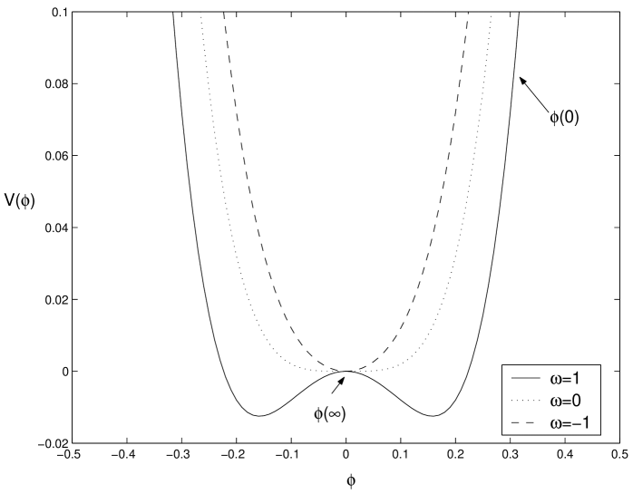
FIG. 1.: The potential $V(\phi)$ is shown for $g=10$ and $\omega=1$.

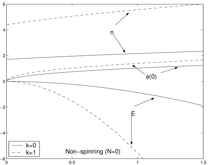
FIG. 2.: The conserved quantities $E$, $n$ and the value $\phi(0)$ are shown as functions of $\omega$ for the non-spinning solutions with $k=0$, $k=1$, respectively.

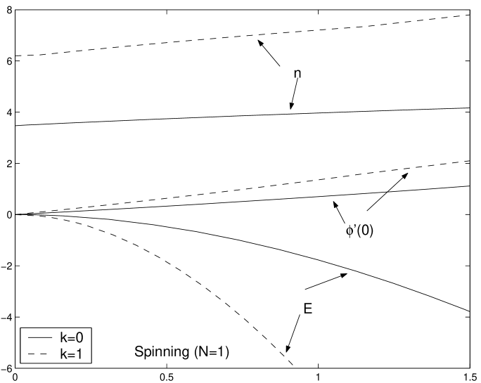
FIG. 3.: The conserved quantities $E$, $n$ and the value $\phi^{\prime}(0)$ are shown as functions of $\omega$ for the spinning solutions ($N=1$) with $k=0$, $k=1$, respectively.

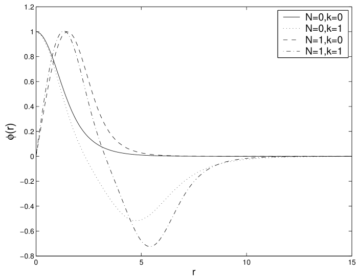
FIG. 4.: The profiles $\phi(r)$ of the soliton solutions are shown for different choices of the node number $k$ and the parameter $N$. $N=0$ are non-spinning solitons. $g=1$.

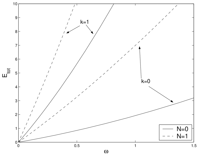
FIG. 5.: The total energy $E_{tot}$ of the non-spinning ($N=0$) and the spinning $(N=1)$ solutions with $k=0,1$ nodes is shown as function of $\omega$

REFERENCES

- [1] R. Rajaraman, Solitons and Instantons, North-Holland Physics Publishing, 1982.
- [2] For a review see e.g. T. D. Lee and Y. Pang, Phys. Rep. 221 (1992), 251.
- [3] S. Coleman, Nucl. Phys. B262 (1985), 263.
- [4] F. E. Schunck and E. W. Mielke, in Relativity and Scientific Computing, Springer, Berlin (1996), 138.
- [5] L. Brizhik, A. Eremko, B. Piette and W. J. Zakrzewski, Physica D 146 (2000), 275.
- [6] L. Brizhik, B. Piette and W. J. Zakrzewski, Ukr. Fiz. Journal 46 (2001), 503.
- [7] L. Brizhik, A. Eremko, B. Piette and W. J. Zakrzewski, Physica D 159 (2001), 71.
- [8] B. Hartmann and W. J. Zakrzewski, Phys. Rev. B 68 (2003), 184302.
- [9] M. Volkov and E. Wöhnert, Phys. Rev. D 66 (2002), 085003.
- [10] M. Volkov and E. Wöhnert, Phys. Rev. D 67 (2003), 105006.
- [11] L. Brizhik, A. Eremko, B. Piette and W. J. Zakrzewski, Nonlinearity 16 (2003), 1481.