hep-th/0308068

Open-Closed Duality: Lessons from Matrix Model

Ashoke Sen

Harish-Chandra Research Institute

Chhatnag Road, Jhusi, Allahabad 211019, INDIA

E-mail: ashoke.sen@cern.ch, sen@mri.ernet.in

Abstract

Recent investigations involving the decay of unstable D-branes in string theory suggest that the tree level open string theory which describes the dynamics of the D-brane already knows about the closed string states produced in the decay of the brane. We propose a specific conjecture involving quantum open string field theory to explain this classical result, and show that the recent results in two dimensional string theory are in exact accordance with this conjecture.

Recent studies involving decay of unstable D-brane systems in string theory indicate that while these D-branes are expected to decay into closed string states of mass of order $1/g_{s}$[1, 2, 3], tree level open string theory provides an alternative description of the same process[4, 5, 6, 7, 8, 9, 10, 11, 12, 13, 14, 15, 16, 17, 18, 19, 20, 21, 22]. In particular various properties of the final state closed strings produced during this decay agree with the predictions based on tree level open string analysis[2, 23, 24, 25]. These properties include the form of the energy-momentum tensor, dilaton charge and anti-symmetric tensor field charge of the system at late time. This suggests that in some way, tree level open string theory already contains information about the final state closed strings produced during this decay[23, 24].

Clearly, in order to put this correspondence into a firmer footing, one needs a specific proposal for the full quantum theory. We propose the following

Conjecture: There is a quantum open string field theory (OSFT) that describes the full dynamics of an unstable Dp-brane without an explicit coupling to closed strings. Furthermore, Ehrenfest theorem holds in the weakly coupled OSFT: the classical results correctly describe the evolution of the quantum expectation values.

According to this conjecture, the effect of closed string emission is already contained in the full quantum OSFT, and furthermore, in the weak coupling limit, the results of quantum OSFT must approach the results in classical OSFT. Thus the above conjecture is sufficient to explain the observed open closed duality mentioned earlier. For any finite coupling, the Ehrenfest theorem could break down over a sufficiently long time scale, but this time scale should approach infinity in the limit of zero coupling constant.

It is instructive to apply the above conjecture to the specific case of unstable D0-brane system. The quantum OSFT on a D0-brane is a quantum mechanical system of infinitely many degrees of freedom. If the above conjecture is valid, then this quantum mechanical system contains complete description of the closed strings produced in the decay of the D0-brane, even though these closed strings live in the full space-time of string theory, which is (25+1) dimensional for the bosonic string theory and (9+1)-dimensional for the superstring theory.

Note that the conjecture stated above does not imply that the OSFT on a D0-brane (or any D$p$-brane for that matter) contains complete information about all states in string theory. It simply states that the OSFT on the D0-brane is a consistent quantum theory by itself, and hence has included in it a description of the closed string states into which an unstable D0-brane is allowed to decay. In other words, OSFT on an unstable D-brane describes a closed subsector of the full string theory.

At present in the critical string theory there is not much further evidence for this conjecture beyond those already mentioned. The only other piece of information which is relevant is that formally the perturbation expansion of the OSFT around the maximum of the tachyon potential seems to be complete, in the sense that it reproduces correctly the Polyakov amplitudes of the first quantized string theory involving external open string states to all orders in perturbation theory. In particular the amplitude has the correct poles corresponding to intermediate closed string states[33]. This suggests that the quantum OSFT is a consistent quantum theory by itself. Note however that the perturbation expansion discussed above is purely formal, as the amplitudes are divergent due to the presence of the open string tachyonic mode which lives on the unstable D-brane. Nevertheless, the formal consistency of the perturbation theory suggests that the same theory, when quantized correctly by expanding the action around the tachyon vacuum, will give a fully consistent quantum theory, as the tachyonic mode will be absent around such a vacuum.

We can however do much better in the two dimensional string theory for which a specific non-perturbative formulation is available in the form of a matrix quantum mechanics. There are two specific models for which the correspondence has been established, – the two dimensional bosonic string theory[34, 35, 36] and the two dimensional type 0B string theory[37, 38]. Since the matrix models associated with the two systems are very similar, our discussion will be valid for both theories. In order that the various formulæ in the two theories look identical, we shall set $\hbar=c=1$ and choose $\alpha^{\prime}=1$ unit for the bosonic string theory and $\alpha^{\prime}=1/2$ unit for type 0B string theory. In this convention the open string tachyon on the D0-brane has mass${}^{2}=-1$ in both theories. Also we shall define the closed string coupling constant $g_{s}$ in such a way that the D0-brane has mass $1/g_{s}$ in both theories. We shall restrict our discussion mainly to D0-branes in type 0B string theory, since the two dimensional bosonic string theory is believed to be non-perturbatively inconsistent[40, 41, 42, 43].

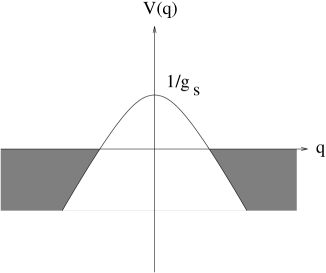
Figure 1: The matrix model description of the vacuum state of type 0B string theory in 1+1 dimensions. All the negative energy states are filled as shown by the shaded region of the diagram.

According to the matrix model - string theory correspondence, the two dimensional type 0B string theory is equivalent to a theory of infinite number of non-interacting fermions, each moving in an inverted harmonic oscillator potential with hamiltonian

$$h(p,q)={1\over 2}(p^{2}-q^{2})+{1\over g_{s}}\,,$$ (1)

where $(q,p)$ denote a canonically conjugate pair of variables. The coordinate variable $q$ is related to the eigenvalue of an infinite dimensional matrix, but this information will not be necessary for our discussion. Clearly $h(p,q)$ has a continuous energy spectrum spanning the range $(-\infty,\infty)$. The vacuum of the theory corresponds to all states with negative $h$ eigenvalue being filled and all states with positive $h$ eigenvalue being empty (see Fig.1). Thus the fermi surface is the surface of zero energy. In the semi-classical limit, in which we represent a quantum state by an area element of size $\hbar$ in the phase space spanned by $p$ and $q$, we can represent the vacuum by having the region $(p^{2}-q^{2})\leq-{2\over g_{s}}$ filled, and rest of the region empty[44, 45]. This has been shown in Fig.2. Thus in this picture the fermi surface in the phase space corresponds to the curve:

$${1\over 2}(p^{2}-q^{2})+{1\over g_{s}}=0\,.$$ (2)

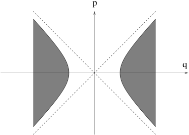
Figure 2: Semi-classical representation of the vacuum state in the matrix model.

It has been realized recently[46, 47, 48, 49, 50, 37, 38] that D0-branes in two dimensional string theory[51, 52, 53] also have simple description in the matrix model. In particular, a state of a single D0-brane of the theory corresponds to a single fermion excited from the fermi surface to some energy above zero. Since the fermions are non-interacting, these states do not mix with any other states in the theory (say with states where two or more fermions are excited above the fermi level or states where a fermion is excited from below the fermi level to the fermi level). As a result, the quantum states of a D0-brane are in one to one correspondence with the quantum states of the Hamiltonian $h(p,q)$ given in (1) with one crucial difference, – the spectrum is cut off sharply for energy below zero due to Pauli exclusion principle. Thus in the matrix model description, the quantum ‘open string field theory’ for a single D0-brane is described by the inverted harmonic oscillator hamiltonian (1) with all the negative energy states removed by hand. The classical limit of this quantum Hamiltonian is described by the classical Hamiltonian (1), with a sharp cut-off on the phase space variables:

$${1\over 2}(p^{2}-q^{2})+{1\over g_{s}}\geq 0\,.$$ (3)

This is the matrix model description of classical ‘open string field theory’ describing the dynamics of a D0-brane.

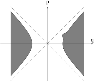
Figure 3: Semiclassical representation of a closed string field configuration in the matrix model.

Clearly the quantum system described above provides us with a complete description of the dynamics of a single D0-brane. This is in accordance with the general conjecture put forward at the beginning of this note. Note in particular that there is no need to couple this system explicitly to closed strings. In this context we note that according to [44, 45], classical closed string field configurtions in this theory correspond to deformations of the fermi surface (2) in the phase space (see Fig.3). In contrast the semi-classical description of a D0-brane with energy of order $1/g_{s}$ amounts to filling up an area of order $\hbar$ in the phase space at an energy of order $1/g_{s}$ above the fermi surface (see Fig.4), and hence such a state cannot be described as a deformation of the fermi surface. Thus in general a D0-brane cannot be described as a classical closed string field configuration. However in the asymptotic past and asymptotic future all trajectories in the phase space, including the fermi surface, approach the asymptotes $p=\pm q$. Thus in this limit the D0-brane can be thought of as a deformation of the fermi surface, i.e. a classical closed string field configuration[45]. The precise form of this closed string field configuration can be found using the bosonization formula[54, 55, 56] and was shown to agree[50, 37, 38, 49, 57] with the coherent closed string fields produced in the decay of the D0-brane computed directly from the continuum string theory[1, 2]. This is one of the compelling pieces of evidence that the identification of the D0-brane with the single excited fermion in the matrix model description is correct. But this also clearly demonstrates that closed strings produced in the ‘decay’ of the D0-brane are already included in the quantum ‘open string field theory’ describing the dynamics of the D0-brane, and there is no need to take into account the closed string emission effect separately.

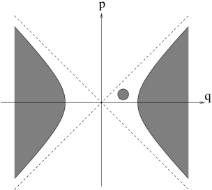
Figure 4: Semi-classical representation of a state of the D0-brane in the matrix model.

It remains to see how this simple system described by the Hamiltonian (1) with the phase space cut-off (3) is related to the more conventional description of the continuum open string field theories (OSFT) of the type described in [28] and [30, 31, 32]. To this end we note the following facts:

1. The effective Planck’s constant (coupling constant) of the single fermion quantum mechanics described in (1) is of order $g_{s}$[44]. This can be seen by introducing new variables $\widetilde{p}=\sqrt{g_{s}}p$, $\widetilde{q}=\sqrt{g_{s}}q$ so that the Hamiltonian expressed in terms of $\widetilde{p}$, $\widetilde{q}$ has an overall multiplicative factor of $1/g_{s}$, but otherwise there is no $g_{s}$ dependence either in the Hamiltonian or in the constraint (3). The commutator of $\widetilde{q}$ and $\widetilde{p}$ is proportional to $ig_{s}$, and hence in terms of the rescaled variables $g_{s}$ is the effective Planck’s constant. On the other hand in the standard OSFT also $g_{s}$ is the effective Planck’s constant since $1/g_{s}$ appears as an overall multiplicative factor in the action. Thus we see that $g_{s}$ plays the same role in the quantum OSFT and the quantum system described by (1), (3).

2. Both the classical Hamiltonian (1) with the constraint (3) and the OSFT on a D0-brane have a lower bound of zero on the energy[31, 32, 58, 59, 60, 61, 62, 63].

3. Next we shall compare time dependent classical solutions in the OSFT on a D0-brane and the system described by (1), (3). During this discussion we shall assume that given any boundary conformal field theory (BCFT) obtained by deforming the original D0-brane BCFT by a marginal deformation, we have a classical solution of the OSFT. We should caution the reader however that explicit construction of these solutions may involve subtle issues, and so far a clear correpondence between BCFT and the classical solutions of OSFT have not been established in the context of time dependent solutions[18, 19].

   Comparing the classical solutions of the equations of motion derived from the Hamiltonian (1) subject to the constraint (3), and the BCFT’s describing time dependent configurations on a D0-brane, we find that both systems have a continuous family of solutions labelled by the energy $E$ for all $E\geq 0$. In fact for each energy there are two inequivalent orbits. In the case of the system described by (1), (3), these solutions are given by:

   $$q=\pm\sqrt{2(g_{s}^{-1}-E)}\,\cosh(x^{0}),\quad p=\pm\sqrt{2(g_{s}^{-1}-E)}\,\sinh(x^{0}),\quad\hbox{for $0\leq E\leq g_{s}^{-1}$}\,,$$

   $$q=\pm\sqrt{2(E-g_{s}^{-1})}\,\sinh(x^{0}),\quad p=\pm\sqrt{2(E-g_{s}^{-1})}\,\cosh(x^{0}),\quad\hbox{for $E\geq g_{s}^{-1}$}\,.$$

   Here $x^{0}$ is the time coordinate. On the other hand in OSFT for D0-branes in the continuum type 0B string theory, these solutions correspond to adding to the world-sheet theory a boundary deformation proportional to[5]

   $$\pm\widetilde{\lambda}\Psi^{0}\,\sinh(X^{0})\otimes\sigma_{1},\quad\widetilde{\lambda}=\cos^{-1}(\sqrt{Eg_{s}}),\quad 0\leq\widetilde{\lambda}\leq{1\over 2},\quad\hbox{for $0\leq E\leq g_{s}^{-1}$}\,,$$

   $$\pm\widetilde{\lambda}\Psi^{0}\cosh(X^{0})\otimes\sigma_{1},\quad\widetilde{\lambda}=\cosh^{-1}(\sqrt{Eg_{s}}),\quad\widetilde{\lambda}\geq 0,\quad\hbox{for $E\geq g_{s}^{-1}$}\,.$$ (5)

   Here $X^{0}$ is the world-sheet field corresponding to the time coordinate, $\Psi^{0}$ denotes the world-sheet superpartner of $X^{0}$ and $\sigma_{1}$ is a Chan-Paton factor. In both the matrix model description based on (1), (3) and the continuum string theory description, each of these orbits are open orbits, i.e. they are not periodic. Thus the two theories have exactly the same family of classical solutions.

   If classical OSFT could be viewed as a Hamiltonian system described by a pair of phase space coordinates $(T,\Pi)$ with some Hamioltonian $H(\Pi,T)$ (e.g. $H=\sqrt{\Pi^{2}+(V(T))^{2}}$ with $V(T)=1/(g_{s}\cosh T)$ as described in [6, 73, 74, 75, 76, 77, 78, 79, 80, 81, 82, 83, 84]) then the above correspondence between classical solutions would immediately imply that there is a canonical transformation relating this system to the one described by (1), (3). This canonical transformation can be found as follows. Let the trajectories of OSFT for a given energy $E$ be given by

   $$T=F(E,x^{0}),\qquad\Pi=G(E,x^{0})\,,$$ (6)

   and the trajectories of the system described by (1), (3) be given by:

   $$q=f(E,x^{0}),\qquad p=g(E,x^{0})\,.$$ (7)

   We can now eliminate $E$ and $x^{0}$ from eqs.(6) and (7) to express $q$ and $p$ in terms of $T$ and $\Pi$ or vice versa. As long as the orbits are open, this is always possible and gives a one to one mapping between the allowed regions of the $(q,p)$ plane and the $(T,\Pi)$ plane. In particular, if the $(T,\Pi)$ coordinates are unconstrained, – as in the case of the tachyon ‘effective Hamiltonian’ $H=\sqrt{\Pi^{2}+1/(g_{s}^{2}\cosh^{2}T)}$, – then the region (3) will be mapped to the full $(T,\Pi)$ plane. The transformation constructed this way is also guaranteed to be canonical, and maps $H(\Pi,T)$ to $h(p,q)$. Thus the two systems are related by canonical transformation. (In contrast if the orbits had been periodic, such a transformation can be constructed only if the periods of the orbit for any given energy $E$ are identical in the two systems.)

   Unfortunately OSFT in its current form cannot be thought of as a Hamiltonian system since it has interaction terms involving higher order time derivatives. Nevertheless, the fact that the classical solutions in the two systems are in one to one correspondence strongly suggests that the two systems are classically equivalent.

4. We can also compare the set of classical solutions in the euclidean version of the two theories. While the euclidean solutions are not directly relevant for comparing the two classical theories in the Lorentzian signature space-time, in the quantum theory these euclidean solutions induce tunnelling between two sides of the tachyon potential for orbits with $E<g_{s}^{-1}$, and hence comparing them between the two theories is important for establishing the equivalence between the two quantum theories[50, 38]. Euclideanization of the system described by (1), (3) is achieved by making the replacement $p\to ip$, $x^{0}\to ix$ in the classical solutions and the constraint (3). Thus the inequivalent classical solutions in this theory are:

   $$q=\lambda\cos x,\qquad p=\lambda\sin x,\qquad\lambda^{2}<{2\over g_{s}}\,.$$ (8)

   On the other hand in the continuum string theory the euclidean solutions are obtained as boundary deformation of the world-sheet theory with $X^{0}$ and $\Psi^{0}$ replaced by $iX$ and $i\Psi$ respectively. The inequivalent classical solutions on a D0-brane in continuum type 0B string theory correspond to deformation by[85, 86]

   $$\widetilde{\lambda}\Psi\sin X\otimes\sigma_{1},\qquad 0\leq\widetilde{\lambda}\leq{1\over 2}\,.$$ (9)

   The important point to note is that in both the matrix theory version and the continuum version the solutions are periodic in euclidean time coordinate $x$ with the same (energy independent) periodicity $2\pi$. Thus even in the euclidean theory the classical solutions of the system described by (1), (3) are in one to one correspondence to the classical solutions of OSFT. Had OSFT been described by a canonical Hamiltonian this would imply that the semiclassical tunnelling probability $P(E)$ for tunnelling across the potential barrier at any given energy $E$ is identical in OSFT and the matrix model, – $P(E)\sim\exp[-2\pi({1\over g_{s}}-E)]$, – since for a canonical system $P(E)$ is determined in terms of the period $\tau(E)$ of the euclidean orbit via the relation $\tau(E)={d\over dE}\ln P(E)$. (In this context note that the tachyon ‘effective Hamiltonian’ $H=\sqrt{\Pi^{2}+1/(g_{s}^{2}\cosh^{2}T)}$ also has orbits of the same period in the Euclidean theory[1]. Hence the semiclassical tunnelling probability across the potential barrier in this theory is identical to that for the system described by (1), (3), i.e. $P(E)\sim\exp[-2\pi({1\over g_{s}}-E)]$.)

   There is however one subtle issue here. The solution associated with $\lambda=\sqrt{2/g_{s}}$ in the matrix model description corresponds to the point $\widetilde{\lambda}={1\over 2}$ in the continuum OSFT description. Physically in the continuum theory this solution represents a periodic array of D-instanton - anti-D-instanton pair with periodicity $2\pi$. But given this configuration, we can deform it to construct other solutions of the Euclidean OSFT where the array has a different periodicity. In fact we can construct a family of solutions parametrized by the periodicity[2], and in the limit of infinite periodicity we have a single isolated D-instanton. The matrix model counterpart does not seem to have these solutions. The resolution of this puzzle could lie in the fact that while the quantum mechanics of a single D0-brane system is well defined in the matrix model description, the semi-classical limit may break down very close to the Fermi level due to the sharp cut-off on the energy levels. Thus in the $g_{s}\to 0$ limit the classical Hamiltonian (1) with the constraint (3) may not be the correct description of the system very close to the fermi level (2). It is precisely at the (euclidean version of the) fermi level that a new direction of deformation opens up for the OSFT solution. It is clearly important to investigate this issue in detail.

The various tests described above provide strong evidence that the full quantum OSFT on a single D0-brane is equivalent to the quantum theory of a single particle described by (1), (3). Indeed if the matrix model - string theory correspondence is right, and if the identification of the D0-brane as a single excited fermion is correct, then this must be the case. This, in turn, would imply that quantum OSFT in the continuum (1+1) dimensional string theory is an internally consistent theory and is capable of describing the complete dynamics of the D0-brane, exactly in accordance with the conjecture.

One can easily generalise this discussion to the case of multiple (say $n$) D0-branes. In the matrix model a state of $n$ D0-branes corresponds to $n$ fermions excited from the fermi level to some states above the fermi level. The dynamics of such a system is clearly described by the quantum mechanics of $n$ non-interacting fermions, each moving under the Hamiltonian (1) and satisfying the constraint (3). This is clearly a consistent theory by itself. In the continuum string theory the corresponding OSFT is easily constructed in terms of the boundary conformal field theory of $n$ D0-branes. The matrix model - string theory correspondence would imply that this quantum OSFT is exactly equivalent to the quantum system of $n$ fermions described above. Hence the OSFT describing the dynamics of $n$ D0-branes will be an internally consistent quantum theory. This is again in accordance with our general conjecture. However in general (e.g. in critical string theory) even if the quantum OSFT on $n$ D0-branes provides a complete description of the system, there is no reason for this theory to be physically equivalent to $n$ copies of the OSFT describing a single D0-brane.

We must emphasize again that in each case, the states of the D0-brane system, described by OSFT or the matrix theory hamiltonian (1), (3), describe only a subset of states in string theory. Thus we do not recover the full string theory by studying the OSFT, but recover a subsector of the theory that is a consistent quantum theory by itself. It is this lesson that we expect will be valid in the full critical string theory, and forms the basis of the conjecture stated at the beginning of this note. It is however instructive to ask, in the context of the two dimensional string theory, if there is some D0-brane system that describes the full string theory. To this effect we note that since a state of $n$ D0-branes corresponds in the matrix model to a state where $n$ fermions are excited above the fermi level, as we increase the number $n$ of D0-branes, the system is capable of describing more and more states in the theory. In the $n\to\infty$ limit, the states of the OSFT describe arbitrary excitations of multiple fermions from fermi level to any state above the fermi level. This however leaves out one important class of states, namely the ‘hole states’ where we excite states from below the fermi level to the fermi level. If we had another set of ‘D0-branes’ whose quantum states describe the hole states of the theory, then by beginning with $n$ usual D0-branes and $m$ ‘hole type’ D0-branes, and taking the limit $m,n\to\infty$, we could represent all the states of the matrix model as states of the OSFT on this D0-brane system. Some proposal for the boundary conformal field theory describing the hole states has recently been put forward in [38, 91], but it remains to be seen to what extent the dynamics of these ‘hole type’ D0-branes can be described by the standard open string field theory. Alternatively one might hope that by taking open string field theory on a finite number of space-filling non-BPS branes (or brane anti-brane systems) one might be able to describe all the states of the theory. However since there is not yet a simple description of the space-filling branes in the matrix model, the matrix model does not provide any insight into this possibility.

We should add here that the view about the hole states described above represents perhaps a conservative view of the situation. A more radical viewpoint will be that single hole states can also be represented as states of the same OSFT that describes the D0-brane. The proposal for the hole states outlined in [38, 91] involves analytic continuation in the parameter space of the solution describing a D0-brane and simultaneously changing the sign of the boundary state. It is not clear whether this combined operation generates a solution of the original OSFT, but it is worth examining this issue in detail.

We would like to end with the remark that if the conjecture stated in this note is valid in a general string theory, then we have the possibility of studying different subsectors of string theory associated with different unstable brane systems without having to study the whole string theory at once. This might eventually lead to an efficient way of studying string theory.

Acknowledgement: I would like to thank P. Mukhopadhyay, L. Rastelli, M. Rozali, M. Schnabl and B. Zwiebach for useful discussions, and L. Rastelli and B. Zwiebach for a critical reading of the manuscript. I would also like to thank the Center for Theoretical Physics at MIT, the organisers of the Strings 2003 conference at Kyoto and the Pacific Institute for the Mathematical Sciences at Vancouver for hospitality during various stages of this work.

References

- [1] N. Lambert, H. Liu and J. Maldacena, arXiv:hep-th/0303139.
- [2] D. Gaiotto, N. Itzhaki and L. Rastelli, arXiv:hep-th/0304192.
- [3] B. Chen, M. Li and F. L. Lin, JHEP 0211, 050 (2002) [arXiv:hep-th/0209222].
- [4] A. Sen, JHEP 0204, 048 (2002) [arXiv:hep-th/0203211].
- [5] A. Sen, JHEP 0207, 065 (2002) [arXiv:hep-th/0203265].
- [6] A. Sen, Mod. Phys. Lett. A 17, 1797 (2002) [arXiv:hep-th/0204143].
- [7] A. Sen, JHEP 0210, 003 (2002) [arXiv:hep-th/0207105].
- [8] P. Mukhopadhyay and A. Sen, JHEP 0211, 047 (2002) [arXiv:hep-th/0208142].
- [9] M. Gutperle and A. Strominger, JHEP 0204, 018 (2002) [arXiv:hep-th/0202210].
- [10] A. Strominger, arXiv:hep-th/0209090.
- [11] M. Gutperle and A. Strominger, arXiv:hep-th/0301038.
- [12] A. Maloney, A. Strominger and X. Yin, arXiv:hep-th/0302146.
- [13] T. Okuda and S. Sugimoto, Nucl. Phys. B 647, 101 (2002) [arXiv:hep-th/0208196].
- [14] F. Larsen, A. Naqvi and S. Terashima, JHEP 0302, 039 (2003) [arXiv:hep-th/0212248].
- [15] N. R. Constable and F. Larsen, arXiv:hep-th/0305177.
- [16] S. Sugimoto and S. Terashima, JHEP 0207, 025 (2002) [arXiv:hep-th/0205085].
- [17] J. A. Minahan, JHEP 0207, 030 (2002) [arXiv:hep-th/0205098].
- [18] N. Moeller and B. Zwiebach, JHEP 0210, 034 (2002) [arXiv:hep-th/0207107].
- [19] M. Fujita and H. Hata, arXiv:hep-th/0304163.
- [20] I. Y. Aref’eva, L. V. Joukovskaya and A. S. Koshelev, arXiv:hep-th/0301137.
- [21] S. J. Rey and S. Sugimoto, Phys. Rev. D 67, 086008 (2003) [arXiv:hep-th/0301049].
- [22] S. J. Rey and S. Sugimoto, arXiv:hep-th/0303133.
- [23] A. Sen, arXiv:hep-th/0305011.
- [24] A. Sen, arXiv:hep-th/0306137.
- [25] J. L. Karczmarek, H. Liu, J. Maldacena and A. Strominger, arXiv:hep-th/0306132.
- [26] S. B. Giddings, E. J. Martinec and E. Witten, Phys. Lett. B 176, 362 (1986).
- [27] B. Zwiebach, Commun. Math. Phys. 142, 193 (1991).
- [28] E. Witten, Nucl. Phys. B 268, 253 (1986).
- [29] N. Berkovits and C. T. Echevarria, Phys. Lett. B 478, 343 (2000) [arXiv:hep-th/9912120].
- [30] N. Berkovits, Nucl. Phys. B 450, 90 (1995) [Erratum-ibid. B 459, 439 (1996)] [arXiv:hep-th/9503099].
- [31] N. Berkovits, JHEP 0004, 022 (2000) [arXiv:hep-th/0001084].
- [32] N. Berkovits, A. Sen and B. Zwiebach, Nucl. Phys. B 587, 147 (2000) [arXiv:hep-th/0002211].
- [33] D. Z. Freedman, S. B. Giddings, J. A. Shapiro and C. B. Thorn, Nucl. Phys. B 298, 253 (1988); J. A. Shapiro and C. B. Thorn, Phys. Lett. B 194, 43 (1987); Phys. Rev. D 36, 432 (1987).
- [34] D. J. Gross and N. Miljkovic, Phys. Lett. B 238, 217 (1990).
- [35] E. Brezin, V. A. Kazakov and A. B. Zamolodchikov, Nucl. Phys. B 338, 673 (1990).
- [36] P. Ginsparg and J. Zinn-Justin, Phys. Lett. B 240, 333 (1990).
- [37] T. Takayanagi and N. Toumbas, arXiv:hep-th/0307083.
- [38] M. R. Douglas, I. R. Klebanov, D. Kutasov, J. Maldacena, E. Martinec and N. Seiberg, arXiv:hep-th/0307195.
- [39] I. R. Klebanov, arXiv:hep-th/9108019.
- [40] G. W. Moore, Nucl. Phys. B 368, 557 (1992).
- [41] G. W. Moore, M. R. Plesser and S. Ramgoolam, Nucl. Phys. B 377, 143 (1992) [arXiv:hep-th/9111035].
- [42] J. Polchinski, arXiv:hep-th/9411028.
- [43] A. Dhar, G. Mandal and S. R. Wadia, Nucl. Phys. B 454, 541 (1995) [arXiv:hep-th/9507041].
- [44] J. Polchinski, Nucl. Phys. B 362, 125 (1991).
- [45] A. Dhar, G. Mandal and S. R. Wadia, Int. J. Mod. Phys. A 8, 3811 (1993) [arXiv:hep-th/9212027].
- [46] E. J. Martinec, arXiv:hep-th/0305148.
- [47] S. Y. Alexandrov, V. A. Kazakov and D. Kutasov, arXiv:hep-th/0306177.
- [48] J. McGreevy and H. Verlinde, arXiv:hep-th/0304224.
- [49] J. McGreevy, J. Teschner and H. Verlinde, arXiv:hep-th/0305194.
- [50] I. R. Klebanov, J. Maldacena and N. Seiberg, JHEP 0307, 045 (2003) [arXiv:hep-th/0305159].
- [51] A. B. Zamolodchikov and A. B. Zamolodchikov, arXiv:hep-th/0101152.
- [52] T. Fukuda and K. Hosomichi, Nucl. Phys. B 635, 215 (2002) [arXiv:hep-th/0202032].
- [53] C. Ahn, C. Rim and M. Stanishkov, Nucl. Phys. B 636 (2002) 497 [arXiv:hep-th/0202043].
- [54] S. R. Das and A. Jevicki, Mod. Phys. Lett. A 5, 1639 (1990).
- [55] A. M. Sengupta and S. R. Wadia, Int. J. Mod. Phys. A 6, 1961 (1991).
- [56] D. J. Gross and I. R. Klebanov, Nucl. Phys. B 352, 671 (1991).
- [57] M. Gutperle and P. Kraus, hep-th/0308047.
- [58] P. J. De Smet and J. Raeymaekers, JHEP 0005, 051 (2000) [arXiv:hep-th/0003220].
- [59] A. Iqbal and A. Naqvi, arXiv:hep-th/0004015.
- [60] D. Kutasov, M. Marino and G. W. Moore, arXiv:hep-th/0010108.
- [61] P. Kraus and F. Larsen, Phys. Rev. D 63, 106004 (2001) [arXiv:hep-th/0012198].
- [62] T. Takayanagi, S. Terashima and T. Uesugi, JHEP 0103, 019 (2001) [arXiv:hep-th/0012210].
- [63] D. Ghoshal, arXiv:hep-th/0106231.
- [64] V. A. Kostelecky and S. Samuel, Nucl. Phys. B 336, 263 (1990).
- [65] V. A. Kostelecky and R. Potting, Phys. Lett. B 381, 89 (1996) [arXiv:hep-th/9605088].
- [66] A. Sen and B. Zwiebach, JHEP 0003, 002 (2000) [arXiv:hep-th/9912249].
- [67] N. Moeller and W. Taylor, Nucl. Phys. B 583, 105 (2000) [arXiv:hep-th/0002237].
- [68] W. Taylor, JHEP 0303, 029 (2003) [arXiv:hep-th/0208149].
- [69] D. Gaiotto and L. Rastelli, arXiv:hep-th/0211012.
- [70] A. A. Gerasimov and S. L. Shatashvili, JHEP 0010, 034 (2000) [arXiv:hep-th/0009103].
- [71] D. Kutasov, M. Marino and G. W. Moore, JHEP 0010, 045 (2000) [arXiv:hep-th/0009148].
- [72] D. Ghoshal and A. Sen, JHEP 0011, 021 (2000) [arXiv:hep-th/0009191].
- [73] A. Sen, JHEP 9910, 008 (1999) [arXiv:hep-th/9909062].
- [74] M. R. Garousi, Nucl. Phys. B 584, 284 (2000) [arXiv:hep-th/0003122]. Nucl. Phys. B 647, 117 (2002) [arXiv:hep-th/0209068]. arXiv:hep-th/0303239; arXiv:hep-th/0304145.
- [75] E. A. Bergshoeff, M. de Roo, T. C. de Wit, E. Eyras and S. Panda, JHEP 0005, 009 (2000) [arXiv:hep-th/0003221].
- [76] J. Kluson, Phys. Rev. D 62, 126003 (2000) [arXiv:hep-th/0004106].
- [77] G. W. Gibbons, K. Hori and P. Yi, Nucl. Phys. B 596, 136 (2001) [arXiv:hep-th/0009061].
- [78] A. Sen, arXiv:hep-th/0209122.
- [79] C. j. Kim, H. B. Kim, Y. b. Kim and O. K. Kwon, arXiv:hep-th/0301076.
- [80] F. Leblond and A. W. Peet, arXiv:hep-th/0303035.
- [81] D. Kutasov and V. Niarchos, arXiv:hep-th/0304045.
- [82] G. Gibbons, K. Hashimoto and P. Yi, JHEP 0209, 061 (2002) [arXiv:hep-th/0209034].
- [83] O. K. Kwon and P. Yi, arXiv:hep-th/0305229.
- [84] G. N. Felder, L. Kofman and A. Starobinsky, JHEP 0209, 026 (2002) [arXiv:hep-th/0208019].
- [85] A. Sen, JHEP 9809, 023 (1998) [arXiv:hep-th/9808141].
- [86] A. Sen, JHEP 9812, 021 (1998) [arXiv:hep-th/9812031].
- [87] C. G. Callan, I. R. Klebanov, A. W. Ludwig and J. M. Maldacena, Nucl. Phys. B 422, 417 (1994) [arXiv:hep-th/9402113].
- [88] J. Polchinski and L. Thorlacius, Phys. Rev. D 50, 622 (1994) [arXiv:hep-th/9404008].
- [89] A. Recknagel and V. Schomerus, Nucl. Phys. B 545, 233 (1999) [arXiv:hep-th/9811237].
- [90] A. Sen, Int. J. Mod. Phys. A 14, 4061 (1999) [arXiv:hep-th/9902105].
- [91] D. Gaiotto, N. Itzhaki and L. Rastelli, arXiv:hep-th/0307221.