Multi-dimensional classical and quantum cosmology: Exact solutions, signature transition and stabilization

Abstract

We study the classical and quantum cosmology of a $(4+d)$-dimensional spacetime minimally coupled to a scalar field and present exact solutions for the resulting field equations for the case where the universe is spatially flat. These solutions exhibit signature transition from a Euclidean to a Lorentzian domain and lead to stabilization of the internal space, in contrast to the solutions which do not undergo signature transition. The corresponding quantum cosmology is described by the Wheeler-DeWitt equation which has exact solutions in the mini-superspace, resulting in wavefunctions peaking around the classical paths. Such solutions admit parametrizations corresponding to metric solutions of the field equations that admit signature transition.
PACS numbers: 04.20.-q, 040.50.+h, 040.60.-m

1 Introduction

The interest in multi-dimensional cosmology has its roots in the Kaluza-Klein (KK) idea of geometric unification of interactions and has been a source of inspiration for numerous authors over its long history [1]. Traditionally, the extra dimension in KK theories are assumed to be periodic and can be made arbitrarily small (of the order of the Plank length), being curled up into a closed topology and hence undetectable. However, the relaxation of this condition has caused interesting physics to appear over the past few years in the form of theories which may be categorized as having large extra dimensions. A flood of papers have appeared to address various consequences of having large extra dimensions, motivated by the work of Randall-Sundrum [2] and Arkani-Hamed et.al. [3]. In the former, the authors investigated a string theory inspired $5D$ Anti-de-Sitter (AdS) bulk where our universe appears as an embedded $4D$ singular hypersurface or a 3-brane. In the latter however, a multi-dimensional theory is considered as the fundamental theory in which the scale of gravity is taken to be the gauge unification scale rather than $M_{pl}$ in $4+d$ dimensions where $d$ represents the number of extra dimensions. A notable achievement of these investigations has been to offer a possible explanation for the resolution of the hierarchy problem; the huge disparity in size between various fundamental constants in nature. Yet another approach to models with a large extra dimension comes from the Space-Time-Matter (STM) theory where our $4D$ world is embedded in a $5D$ manifold devoid of matter [4]. In this theory, the matter in $4D$ results from purely geometrical considerations in $5D$, providing us with a theory offering a possible explanation of the origin of matter in the universe. The question of the detection of these extra dimension will have to be addressed in the future, perhaps in an indirect way using high energy particle accelerators.

The class of problems dealing with higher dimensional cosmology with a compactified extra dimension have been used by some authors to address issues like signature transition in classical and quantum cosmology [6]. It would then seem natural to investigate the same issues in theories with large extra dimensions. Naturally, the problem of the stabilization of these extra dimensions and its relation to signature transition would also be the questions worth investigating. This is in contrast to the Randall-Sundrum brane-world scenarios where issues like signature transition and quantum cosmology are fraught with subtleties. For example, in the brane-world scenarios, signature transition has been shown to be incompatible with the $Z_{2}$ symmetry, an important, though not a necessary feature of the theory. Also, in studying the quantum cosmology of such models the question arises as to should one consider the bulk first and the creation of the brane later or should they both come into being at the same time. For a more detailed discussion of the above issues, the reader is referred to [5].

In a multi-dimensional cosmology, a question of interest is that of the stabilization of the extra dimensions and various methods have been employed to address this issue. For example, in [7] stabilization is achieved by using a Casimir-like potential, or in [8] by using a scalar field having an effective potential with a global minimum. The same goal has been achieved in [9] via a balance between vacuum energy, guage fields and the curvature of the internal space.

In this paper, we have considered a multi-dimensional cosmology minimally coupled to a scalar field, described by a potential possessing a global minimum. This feature turns out to be essential in the study of signature transition and stabilization in our model. The presence of a scalar field in the action in the bulk space is generally required for the dynamical stabilization of the theory [12, 8]. Also, the scalar field plays the double role of providing an effective mass to the radion field during inflation and acting as an inflaton which essentially reheats the Universe before nucleosynthesis. Such a potential has previously been used in the context of a $4D$ Friedmann-Robertson-Walker (FRW) cosmology where a self-interacting scalar field is coupled to Einstein’s field equations with a potential containing a Sinh-Gordon scalar interaction [10]. For the case of a spatially flat universe, these equations are then solved exactly for the scalar field and the scale factor as dynamical variables, giving rise to cosmological solutions with a degenerate metric, describing a continuous signature transition from a Euclidean domain to a Lorentzian spacetime. The case for a non-flat universe is addressed in [11]. The scalar field potential used in the present work is that given in [10]. As it turns out, the scalar field plays another role, namely, limiting the number of the internal degrees of freedom.

The paper is organized as follows: In section two the salient features of the model is presented and contact is made to address the hierarchy problem. Section three is devoted to the solution of the field equations and the resulting classical cosmology with a discussion of signature transition. Section four deals with the question of stabilization while in section five the quantum cosmology of the model is studied by presenting solutions to Wheeler-Dewitt (WD) equation. In the last section conclusions are drawn.

2 The Model

Let us start by considering a cosmological model in which the spacetime is assumed to be of Freedmann-Robertson-Walker type with a $d$-dimensional internal space. We adopt a chart $\{\beta,x^{i},x^{\mu}\}$ where $\beta,x^{i}$ and $x^{\mu}$ $(i=1,2,3;\mu=4,\cdots,d+4)$ represent the laps function, the external space coordinates and the internal space coordinates respectively. The metric is given by

$$g=-\beta d\beta\otimes d\beta+\frac{{\bar{R}}^{2}(\beta)}{[1+(\frac{k}{4})r^{2}]^{2}}dx^{i}\otimes dx^{i}+{\bar{a}}^{2}(\beta)g^{(d)}$$ (1)

defined on a bulk manifold with warped product topology

$$M=M_{3+1}\times M_{d}$$

with $D=4+d$ being the total number of dimensions, $k=1,0,-1$ representing the usual spatial curvature, $\bar{R}(\beta)$ and $\bar{a}(\beta)$ are the scale factor of the universe and the radius of the $d$-dimensional internal space respectively and $g^{(d)}$ is the metric for the internal space, assumed to be Ricci-flat. We write the action functional as

$${\cal S}=\frac{1}{2{\kappa_{D}}^{2}}\int_{M}d^{D}x\sqrt{-g}{\cal R}[g]-\frac{1}{2}\int_{M}d^{D}x\sqrt{-g}\left[-\left(\frac{\partial{\tilde{\phi}}}{\partial{\beta}}\right)^{2}+2U(\tilde{\phi})\right]+{\cal S}_{YGH}$$ (2)

where $\kappa_{D}$ is the $D$-dimensional gravitational constant, $\tilde{\phi}$ is a minimally coupled homogeneous scalar field with the potential $U(\tilde{\phi})$ and ${\cal S}_{YGH}$ is the usual York-Gibbons-Hawking boundary term [13]. The signature of the metric (1) is Lorentzian for $\beta>0$ and Euclidean for $\beta<0$. For positive values of $\beta$ one can recover the cosmic time by setting $t=\frac{2}{3}{\beta}^{\frac{3}{2}}$ and the corresponding metric becomes

$$g=-dt\otimes dt+\frac{R^{2}(t)}{[1+(\frac{k}{4})r^{2}]^{2}}dx^{i}\otimes dx^{i}+a^{2}(t)g^{(d)}$$ (3)

where $R(t)=\bar{R}(\beta(t))$ and $a(t)=\bar{a}(\beta(t))$ in the $\{t,x^{i},x^{\mu}\}$ chart. We solve our differential equations in a region that dose not include $\beta=0$ and seek real solutions for $R$ and $a$ passing smoothly through the $\beta=0$ hypersurface. The Ricci scalar corresponding to metric (3) is

$${\cal R}=6\left[\frac{\ddot{R}}{R}+\frac{k+{\dot{R}}^{2}}{R^{2}}\right]+2d\frac{\ddot{a}}{a}+d(d-1)\left(\frac{\dot{a}}{a}\right)^{2}+6d\frac{\dot{a}\dot{R}}{aR}$$ (4)

where a dot represents differentiation with respect to t. Let $a_{0}$ be the compactification scale of the internal space at the present time and

$$\upsilon_{d}\equiv\upsilon_{0}\times\upsilon_{i}\equiv{a_{0}}^{d}\times\int_{M_{d}}d^{d}x\sqrt{-g^{(d)}}$$

the corresponding total volume of the internal space. After dimensional reduction, action (2) becomes

$${\cal S}=-\upsilon_{3}\int dt\left\{6{\dot{R}}^{2}\Phi R+6\dot{R}\dot{\Phi}R^{2}+\frac{d-1}{d}\frac{{\dot{\Phi}}^{2}}{\Phi}R^{3}-6k\Phi R+{\kappa_{0}}^{2}\Phi R^{3}\left(2V(\phi)-{\dot{\phi}}^{2}\right)\right\}$$ (5)

where

$$\Phi=\frac{1}{2{\kappa_{0}}^{2}}\left(\frac{a}{a_{0}}\right)^{d}$$

and we have redefined the scalar field $\tilde{\phi}$ and its associated potential as follows

$$\phi=\sqrt{\upsilon_{d}}\tilde{\phi},\hskip 17.07182ptV(\phi)=\upsilon_{d}U(\phi/\sqrt{\upsilon_{d}})$$

with $\upsilon_{3}$ being the volume of the external spatial space.

At this point, it is appropriate to make contact with the hierarchy problem, mentioned in the introduction [14]. In action (5), $\kappa_{0}$ is the 4-dimensional gravitational constant defined as

$${\kappa_{0}}^{2}=\frac{8\pi}{M^{2}_{Pl}}:=\frac{\kappa^{2}_{D}}{\upsilon_{d}}$$ (6)

where $M_{Pl}=1.22\times 10^{19}$ Gev. The conventional radius of compactification in string theory is of order $L_{Pl}$, resulting in a 10-dimensional gravity scale comparable to the 4-dimensional plank scale. If we normalize $\kappa^{2}_{D}$ in such a way that $\kappa^{2}_{D}=8\pi/M^{2+d}_{EW}$, where $M_{EW}$ is the Standard Model Electroweak scale, then $a_{0}\sim 10^{32/d-17}$ cm, assuming $\upsilon_{i}=1$. This points to a possible solution of the hierarchy problem, different from grand unified and supersymmetric theories.

3 Classical cosmology and exact solutions

From action (5), the effective Lagrangian becomes

$${\cal L}=-6\left\{{\dot{R}}^{2}\Phi R+\dot{R}\dot{\Phi}R^{2}+\frac{d-1}{6d}\frac{{\dot{\Phi}}^{2}}{\Phi}R^{3}-k\Phi R+\frac{1}{3}{\kappa_{0}}^{2}\Phi R^{3}\left(V(\phi)-\frac{\dot{\phi}^{2}}{2}\right)\right\}$$ (7)

where we have set $\upsilon_{3}=1$. The variation of the above Lagrangian yields the Einstein field equations and the equation of motion of the scalar field

$$2\frac{\dot{\Phi}\dot{R}}{\Phi R}+\left(\frac{\dot{R}}{R}\right)^{2}+2\frac{\ddot{R}}{R}+\frac{\ddot{\Phi}}{\Phi}+\frac{k}{R^{2}}-\frac{d-1}{2d}\left(\frac{\dot{\Phi}}{\Phi}\right)^{2} = {\kappa_{0}}^{2}\left(V-\frac{1}{2}\dot{\phi}^{2}\right)$$ (8)

$$3\left[\left(\frac{\dot{R}}{R}\right)^{2}+\frac{\ddot{R}}{R}+\frac{k}{R^{2}}\right]+\frac{d-1}{2d}\left[2\frac{\ddot{\Phi}}{\Phi}-\left(\frac{\dot{\Phi}}{\Phi}\right)^{2}+6\frac{\dot{\Phi}\dot{R}}{\Phi R}\right] = {\kappa_{0}}^{2}\left(V-\frac{1}{2}\dot{\phi}^{2}\right)$$ (9)

$$3\left[\left(\frac{\dot{R}}{R}\right)^{2}+\frac{\dot{\Phi}\dot{R}}{\Phi R}+\frac{k}{R^{2}}\right]+\frac{d-1}{2d}\left(\frac{\dot{\Phi}}{\Phi}\right)^{2} = {\kappa_{0}}^{2}\left(V+\frac{1}{2}\dot{\phi}^{2}\right)$$ (10)

$$\ddot{\phi}+3\frac{\dot{R}\dot{\phi}}{R}+\frac{\dot{\Phi}\dot{\phi}}{\Phi}+\frac{\partial{V}}{\partial{\phi}} = 0.$$ (11)

To make the Lagrangian (7) manageable, consider the the following change of variable

$$\Phi R^{3}=mu^{2}+m^{\prime}v^{2}+2nuv$$

where $m$ , $m^{\prime}$ and $n$ are constants and $R=R(u,v),\Phi=\Phi(u,v)$ are functions of new variables $u,v$. For $mm^{\prime}-n^{2}\neq{0}$ , we assume

$$\left\{\begin{array}[]{l}\vspace{.2 cm}{\Phi}^{\rho_{+}}R^{\sigma_{-}}=c_{1}u+c_{2}v\\ {\Phi}^{\rho_{-}}R^{\sigma_{+}}=c_{3}u+c_{4}v\end{array}\right.$$ (14)

where $c_{1}=pc_{4}$ , $c_{3}=m/pc_{4}$ and $c_{2}=m^{\prime}/c_{4}$ such that $p=n/m^{\prime}\pm\sqrt{(\frac{n}{m^{\prime}})^{2}-m/m^{\prime}}$ and

$$\left\{\begin{array}[]{l}\vspace{.2 cm}\sigma_{\pm}=\frac{1}{2}\left(3\mp\frac{1}{\sqrt{\frac{d+2}{3d}}}\right)\\ \rho_{\pm}=\frac{1}{2}\pm\frac{3}{4}\sqrt{\frac{d+2}{3d}}\mp\frac{1}{4\sqrt{\frac{d+2}{3d}}}.\end{array}\right.$$ (17)

Using the above transformations and concentrating on $k=0$, the Lagrangian becomes

$${\cal L}=-4\left(\frac{d+2}{d+3}\right)\left\{m\dot{u}^{2}+m^{\prime}\dot{v}^{2}+2n\dot{u}\dot{v}+\frac{1}{2}{\kappa_{0}}^{2}\left(\frac{d+3}{d+2}\right)(mu^{2}+m^{\prime}v^{2}+2nuv)(V-\frac{1}{2}\dot{\phi}^{2})\right\}.$$ (18)

Let us define $\zeta$ to be the following vector

$$\zeta=\left(\!\!\begin{array}[]{l}u\cosh(\gamma\phi)\\ v\cosh(\gamma\phi)\\ u\sinh(\gamma\phi)\\ v\sinh(\gamma\phi)\end{array}\!\!\right).$$ (23)

This definition will allow us to write Lagrangian (18) as

$${\cal L}=-\frac{{\kappa_{0}}^{2}}{\gamma^{2}}\left\{\dot{\zeta}^{\top}\Gamma\dot{\zeta}+2\gamma^{2}\zeta^{\top}\Gamma\zeta V\right\}$$ (24)

where $\Gamma=\left(\!\!\!\begin{array}[]{cc}J&\,\,\,0\\ 0&-J\end{array}\!\!\!\right)$, $J=\left(\!\!\!\begin{array}[]{cc}m&n\\ n&m^{\prime}\end{array}\!\!\!\right)$, $\gamma=\frac{\kappa_{0}}{2}\sqrt{\frac{d+3}{d+2}}$ and $\top$ represents transposition. Up to this point the cosmological model has been rather general. However, motivated by the desire to find suitable smooth functions $R(t)$, $\Phi(t)$ and $\phi(t)$, and in particular to stabilize the internal degrees of freedom, we have to specify a suitable potential $V(\phi)$. As has been discussed by various authors [8], stabilization of the internal space can be achieved if the potential has a global minimum with respect to $\phi$. A Potential with such properties has been used in the past [10] in the context of signature transition and we therefore adapt it here for our present purpose. We require that the potential $V(\phi)$ has natural characteristics for small $\phi$, so that we may identify the coefficient of $\frac{1}{2}{\phi}^{2}$ in its Taylor expansion as a positive $M^{2}$ and $V(0)$ as a $D$-dimensional cosmological constant $\Lambda$. In this case the effective Lagrangian can be simplified if we select a potential that satisfies

$$2\gamma^{2}{\zeta}^{\top}\Gamma\zeta V(\phi)={\zeta}^{\top}\Gamma\Sigma\zeta$$ (25)

where $\Sigma=\left(\!\!\!\begin{array}[]{ll}\,\,\,a_{1}&\,\,\,\,b\\ -b&-a_{2}\end{array}\!\!\!\right)$. In terms of $\phi$, (25) implies

$$V(\phi)=\frac{(a_{1}-a_{2})}{4\gamma^{2}}+\frac{(a_{1}+a_{2})}{4\gamma^{2}}\cosh{2\gamma\phi}+\frac{b}{2\gamma^{2}}\sinh{2\gamma\phi}.$$ (26)

Inserting the physical parameters $\Lambda=V|_{\phi=0}=a_{1}/{2\gamma^{2}}$ and $M^{2}=\partial^{2}V/\partial\phi^{2}|_{\phi=0}=a_{1}+a_{2}$ in the potential we find

$$V(\phi)=\Lambda+\frac{1}{2\gamma^{2}}M^{2}\sinh^{2}{\gamma\phi}+\frac{b}{2\gamma^{2}}\sinh{2\gamma\phi}.$$ (27)

The first two terms in (26 ) give rise to a Sinh-Gordon scalar interaction. The third term is interesting since its presence breaks the symmetry of $V$ under $\phi\rightarrow-\phi$ and is directly responsible for the signature changing properties of the solutions to be discussed below. For $|2b/M^{2}|<1$ the potential has a minimum value

$$\Lambda+4M^{2}\gamma^{2}\left(\sqrt{1-\frac{4b^{2}}{M^{4}}}-1\right)\hskip 14.22636pt\mbox{at}\hskip 17.07182pt\phi=-\frac{1}{2\gamma}\tanh^{-1}{\left(\frac{2b}{M^{2}}\right)}.$$ (28)

This minimum is believed to support the stabilization of the internal space degrees of freedom as is discussed below. Now, if we choose normal mode basis that diagonalize $\Sigma$ and write $\zeta=S\alpha(t)$ with

$$S^{-1}\Sigma S=\Sigma_{d}=\left(\!\!\begin{array}[]{ll}\lambda_{+}&0\\ 0&\lambda_{-}\end{array}\!\!\!\!\right)$$ (31)

where

$$S=\left(\!\!\begin{array}[]{cc}\frac{b}{\Omega_{1}}&\frac{b}{\Omega_{2}}\\ \frac{(\lambda_{+}-a_{1})}{\Omega_{1}}&\frac{(\lambda_{-}-a_{1})}{\Omega_{2}}\end{array}\!\!\right)$$ (34)

and

$$\lambda_{\pm}=\frac{1}{2}\left[a_{1}-a_{2}\pm\sqrt{(a_{1}+a_{2})^{2}-4b^{2}}\right]$$

$$\Omega_{1}=\sqrt{b^{2}-(\lambda_{+}-a_{1})^{2}}$$

$$\Omega_{2}=\sqrt{(\lambda_{-}-a_{1})^{2}-b^{2}}$$

the Lagrangian becomes

$${\cal L}=-\frac{{\kappa_{0}}^{2}}{\gamma^{2}}\left\{\dot{\alpha}^{\top}\Gamma\dot{\alpha}+\alpha^{\top}\Gamma\Sigma_{d}\alpha\right\}$$ (35)

with the general solution for the equations of motion given by ($mm^{\prime}-n^{2}\neq 0$)

$$\alpha=\Upsilon_{+}(t)A+\Upsilon_{-}(t)B$$ (36)

where A and B are constant $(4\times 1)$ vectors and $\Upsilon_{\pm}=\mbox{diag}(e^{\pm\omega_{+}t},e^{\pm\omega_{+}t},e^{\pm\omega_{-}t},e^{\pm\omega_{-}t})$ with $\omega_{\pm}=\sqrt{\lambda_{\pm}}$. In terms of these solutions, the constraint equation (10) becomes

$${\cal H}=-\frac{{\kappa_{0}}^{2}}{\gamma^{2}}\left\{\dot{\alpha}^{\top}\Gamma\dot{\alpha}-\alpha^{\top}\Gamma\Sigma_{d}\alpha\right\}=0.$$ (37)

Let us concentrate on the solutions for which $\dot{\alpha}(0)=0$, that is $A=B$. This would then imply

$$\alpha=\left(\!\!\begin{array}[]{c}2A_{1}\cosh(\omega_{+}t)\\ 2A_{2}\cosh(\omega_{+}t)\\ 2A_{3}\cosh(\omega_{-}t)\\ 2A_{4}\cosh(\omega_{-}t)\end{array}\!\!\right).$$ (38)

Equation (37) can now be written as

$$\left(l^{2}{A^{2}_{2}}-{A^{2}_{4}}\right)\left[m\left(\frac{A_{3}}{A_{1}}\right)^{2}+2n\frac{A_{3}}{A_{1}}+m^{\prime}\right]=0$$ (39)

where $l^{2}=\frac{\lambda_{+}}{\lambda_{-}}$. From the vanishing of the first parentheses we have $A_{4}=\epsilon lA_{2}$ with $\epsilon=\pm 1$. Upon using (38) we find

$$\left\{\begin{array}[]{c}\alpha_{2}=\epsilon l\frac{A_{2}}{A_{3}}\alpha_{1}\vspace{.2 cm}\\ \alpha_{4}=\epsilon l\frac{A_{2}}{A_{3}}\alpha_{3}\end{array}\right.$$ (42)

where use has been made of the relation $\zeta_{1}\zeta_{4}=\zeta_{3}\zeta_{2}$ resulting from (23). If we choose an overall scale by setting $A_{1}=1$, then (14), (23) and (42) result in the first class of solutions given by

$$\frac{R}{R_{0}}=\frac{a}{a_{0}}=\left\{\begin{array}[]{cc}\left[\frac{\cosh^{2}(\omega_{+}t)-l^{2}\cosh^{2}(\omega_{-}t)}{\cosh^{2}(\omega_{+}t_{0})-l^{2}\cosh^{2}(\omega_{-}t_{0})}\right]^{\frac{1}{d(d+3)}}&\hskip 71.13188pt\lambda_{+},\lambda_{-}>0\vspace{.2 cm}\\ \left[\frac{\cos^{2}(\omega_{+}t)-l^{2}\cos^{2}(\omega_{-}t)}{\cos^{2}(\omega_{+}t_{0})-l^{2}\cos^{2}(\omega_{-}t_{0})}\right]^{\frac{1}{d(d+3)}}&\hskip 71.13188pt\lambda_{+},\lambda_{-}<0\end{array}\right.$$ (45)

and

$$\phi=\frac{1}{\gamma}\tanh^{-1}\left\{\begin{array}[]{cc}\frac{\frac{(\lambda_{+}-a_{1})}{\Omega_{1}}\cosh(\omega_{+}t)+\frac{(\lambda_{-}-a_{1})}{\Omega_{2}}\epsilon l\cosh(\omega_{-}t)}{b\left[\frac{1}{\Omega_{1}}\cosh(\omega_{+}t)+\frac{\epsilon l}{\Omega_{2}}\cosh(\omega_{-}t)\right]}&\hskip 28.45274pt\lambda_{+},\lambda_{-}>0\vspace{.3 cm}\\ \frac{\frac{(\lambda_{+}-a_{1})}{\Omega_{1}}\cos(\omega_{+}t)+\frac{(\lambda_{-}-a_{1})}{\Omega_{2}}\epsilon l\cos(\omega_{-}t)}{b\left[\frac{1}{\Omega_{1}}\cos(\omega_{+}t)+\frac{\epsilon l}{\Omega_{2}}\cos(\omega_{-}t)\right]}&\hskip 28.45274pt\lambda_{+},\lambda_{-}<0\end{array}\right.$$ (48)

where $R_{0}$ and $a_{0}$ represent the present external and internal scale factors and $t_{0}$ represents the age of the Universe. We also have

$$(2{\kappa_{0}}^{2}{R_{0}}^{d})^{d+3}=\left[2(c_{3}+\frac{c_{4}A_{2}}{l})\right]^{2+(d-3)\sqrt{\frac{d+2}{3d}}}\left[2(c_{1}+\frac{c_{2}A_{2}}{l})\right]^{(d-3)\sqrt{\frac{d+2}{3d}}-2}.$$

If the second factor in (39) vanishes and setting $A_{1}=1$, we obtain the second class of solutions, namely

$$\left\{\begin{array}[]{c}\alpha_{2}=p^{\prime}\alpha_{1}\vspace{.2 cm }\\ \alpha_{4}=p^{\prime}\alpha_{3}\end{array}\right.$$ (51)

where $p^{\prime}=-n/m^{\prime}\pm\sqrt{(n/m^{\prime})^{2}-m/m^{\prime}}$. The corresponding expressions for $R$, $a$ and $\phi$ are given by

$$\frac{R}{R_{0}}=\frac{a}{a_{0}}=\large\left\{\begin{array}[]{cc}\left[\large\frac{\cosh^{2}(\omega_{+}t)-A^{2}_{3}\cosh^{2}(\omega_{-}t)}{\cosh^{2}(\omega_{+}t_{0})-A^{2}_{3}\cosh^{2}(\omega_{-}t_{0})}\right]^{\frac{1}{d(d+3)}}&\hskip 56.9055pt\lambda_{+},\lambda_{-}>0\vspace{.3 cm}\\ \left[\frac{\cos^{2}(\omega_{+}t)-A^{2}_{3}\cos^{2}(\omega_{-}t)}{\cos^{2}(\omega_{+}t_{0})-A^{2}_{3}\cos^{2}(\omega_{-}t_{0})}\right]^{\frac{1}{d(d+3)}}&\hskip 56.9055pt\lambda_{+},\lambda_{-}<0\end{array}\right.$$ (54)

and

$$\phi=\frac{1}{\gamma}\tanh^{-1}\large\left\{\begin{array}[]{cc}\frac{\frac{(\lambda_{+}-a_{1})}{\Omega_{1}}\cosh(\omega_{+}t)+A_{3}\frac{(\lambda_{-}-a_{1})}{\Omega_{2}}\cosh(\omega_{-}t)}{b\left[\frac{1}{\Omega_{1}}\cosh(\omega_{+}t)+\frac{1}{\Omega_{2}}\cosh(\omega_{-}t)\right]}&\hskip 28.45274pt\lambda_{+},\lambda_{-}>0\vspace{.3 cm}\\ \frac{\frac{(\lambda_{+}-a_{1})}{\Omega_{1}}\cos(\omega_{+}t)+A_{3}\frac{(\lambda_{-}-a_{1})}{\Omega_{2}}\cos(\omega_{-}t)}{b\left[\frac{1}{\Omega_{1}}\cos(\omega_{+}t)+\frac{A_{3}}{\Omega_{2}}\cos(\omega_{-}t)\right]}.&\hskip 28.45274pt\lambda_{+},\lambda_{-}<0\end{array}\right.$$ (57)

We also find

$$(2{\kappa_{0}}^{2}{R_{0}}^{d})^{d+3}=\left[2(c_{1}+p^{\prime}c_{2})\right]^{(d-3)\sqrt{\frac{d+2}{3d}}+2}\left[2(c_{3}+p^{\prime}c_{4})\right]^{(d-3)\sqrt{\frac{d+2}{3d}}-2}.$$

The third class of the solutions are obtained when $n^{2}-mm^{\prime}$ is zero. In this case we have

$$\Phi R^{3}=mu^{2}+m^{\prime}v^{2}+2nuv=(\sqrt{m}u+\sqrt{m^{\prime}}v)^{2}:=q^{2}$$ (58)

hence, following the same procedure as for the previous solutions we adapt the following transformations

$$\left\{\begin{array}[]{c}{\Phi}^{\rho_{+}}R^{\sigma_{-}}=q^{2(\sigma_{-}-\delta\rho_{+})/(3-\delta)}\\ {\Phi}^{\rho_{-}}R^{\sigma_{+}}=q^{2(\sigma_{+}-\delta\rho_{-})/(3-\delta)}\end{array}\right.$$ (61)

where $\delta$ is real and $\delta\neq 3$. Let us set $\zeta=\left(\!\!\begin{array}[]{c}q\cosh\gamma^{\prime}\phi\\ q\sinh\gamma^{\prime}\phi\end{array}\!\!\right)$, $j=\left(\!\!\begin{array}[]{cc}1&\,\,0\\ 0&-1\end{array}\!\!\right)$ and for convenience replace $\gamma$ with $\gamma^{\prime}$ in potential (26). The Lagrangian then becomes

$${\cal L}=-\frac{{\kappa_{0}}^{2}}{{\gamma^{\prime}}^{2}}\left\{{\dot{\zeta}}^{\top}j\dot{\zeta}+{\zeta}^{\top}\Sigma_{d}\zeta\right\}$$ (62)

where

$${\gamma^{\prime}}^{2}=\frac{\kappa_{0}^{2}d(3-\delta)^{2}}{24d(1-\delta)+4(d-1)\delta^{2}}.$$

The general solution in the normal mode, $\alpha=S^{-1}\zeta$, is then given by

$$\alpha=\Upsilon_{+}A+\Upsilon_{-}B$$ (63)

where, $A$ and $B$ are constant $2\times 1$ vectors and $\Upsilon_{\pm}=\mbox{diag}(e^{\pm\omega_{+}t},e^{\pm\omega_{-}t})$. If we choose $\dot{\alpha}(0)=0$, the constraint (10) becomes

$${\alpha(0)}^{\top}\Sigma_{d}\alpha(0)=0$$ (64)

and we have $A_{2}=\epsilon lA_{1}$. The solutions are then given by

$$\left\{\begin{array}[]{cc}\alpha_{2}=2A_{1}\epsilon l\cosh({\frac{1}{l}\cosh^{-1}({\frac{\alpha_{1}}{2A_{1}}})})&\hskip 71.13188pt\lambda_{+},\lambda_{-}>0\vspace{.2 cm}\\ \alpha_{2}=2A_{1}\epsilon l\cos({\frac{1}{l}\cos^{-1}({\frac{\alpha_{1}}{2A_{1}}})})&\hskip 71.13188pt\lambda_{+},\lambda_{-}<0\end{array}\right.$$ (67)

and

$$\frac{R}{R_{0}}=\left(\frac{a}{a_{0}}\right)^{-\frac{d}{\delta}}=\left\{\begin{array}[]{cc}\left[\frac{\cosh^{2}(\omega_{+}t)-l^{2}\cosh^{2}(\omega_{-}t)}{\cosh^{2}(\omega_{+}t_{0})-l^{2}\cosh^{2}(\omega_{-}t_{0})}\right]^{\frac{1}{3-\delta}}&\hskip 71.13188pt\lambda_{+},\lambda_{-}>0\vspace{.3 cm}\\ \left[\frac{\cos^{2}(\omega_{+}t)-l^{2}\cos^{2}(\omega_{-}t)}{\cos^{2}(\omega_{+}t_{0})-l^{2}\cos^{2}(\omega_{-}t_{0})}\right]^{\frac{1}{3-\delta}}&\hskip 71.13188pt\lambda_{+},\lambda_{-}<0\end{array}\right.$$ (70)

with

$$\phi=\frac{1}{\gamma}\tanh^{-1}\left\{\begin{array}[]{cc}\frac{\frac{{(\lambda_{+}-a_{1})}}{\Omega_{1}}\cosh(\omega_{+}t)+l\epsilon\frac{(\lambda_{-}-a_{1})}{\Omega_{2}}\cosh((\omega_{-}t)}{b\left[\frac{1}{\Omega_{1}}\cosh(\omega_{+}t)+\frac{\epsilon l}{\Omega_{2}}\cosh(\omega_{-}t)\right]}&\hskip 28.45274pt\lambda_{+},\lambda_{-}>0\vspace{.3 cm}\\ \frac{\frac{(\lambda_{+}-a_{1})}{\Omega_{1}}\cos(\omega_{+}t)+l\epsilon\frac{(\lambda_{-}-a_{1})}{\Omega_{2}}\cos(\omega_{-}t)}{b\left[\frac{1}{\Omega_{1}}\cos(\omega_{+}t)+\frac{\epsilon l}{\Omega_{2}}\cos(\omega_{-}t)\right]}&\hskip 28.45274pt\lambda_{+},\lambda_{-}<0\end{array}\right.$$ (73)

where

$${R_{0}}^{\delta}=2{\kappa_{0}}^{2}.$$ (74)

For this class of solutions we clearly have

$$\frac{a}{a_{0}}=\left(\frac{R}{R_{0}}\right)^{-\frac{\delta}{d}}$$ (75)

in agreement with that found in [15]. It is clear that if the parameters satisfy $V=\frac{\partial V}{\partial\phi}=0$ with $R$, $a$ and $\phi$ being constants, then for $\Sigma$, we have degenerate zero eigenvalues. For such parameters, the cosmological model becomes an eternal cosmology with a single transition from a Euclidean to a Lorentzian domain at $\beta=0$. For positive eigenvalues of $\Sigma$, signature transition dose not occur since the solutions would not be continuous at $\beta=0$. If the product of $\lambda_{+}$ and $\lambda_{-}$ be less than zero, then $l$ becomes imaginary and the constraint equation can not be satisfied with a real solution. With both eigenvalues negative, equations (45), (54) and (70) exhibit a continuous transition from a Euclidean to a Lorentzian domain, see figure 1. As equation (45) shows, $R/R_{0}$ and $a/a_{0}$ have the same form and the values of $\beta$ where $\bar{R}(\beta)=0$ control the location of the branch points of $\bar{R}(\beta)$. In equations (48) and (73) if we choose $\epsilon=-1$ and set $\Lambda=0$, that is, $a_{1}=0$ then the scalar field vanishes at the transition. The singular behavior of the scalar field at the birth and death of the universe is reflected in the behavior of the scalar curvature ${\cal R}$ given by equation (4). As we have shown above, we see from equations (54) and (57) that the values of $A_{3}$ control the locations of the branch points of the the relevant fields, otherwise, the general behavior of the solutions is the same as that discussed above. From equation (74) one sees that due to the size of $R_{0}$, $\delta$ must have negative values and this makes the solutions finite. Figure 1 shows the plot of the scalar field, the scale factor $R$, the internal scale factor $a$ and the curvature scalar $\cal R$, using equations (70) and (73) for some specific values of the parameters. The smooth transition from the negative to positive values of $\beta$ corresponding to signature transition from a Euclidean to a Lorentzian domain is clearly seen.

The solutions presented above also merit the following observations. For the first and second class solutions, one observes that in the region where $\beta<0$, one may encounter another region over which the signs of $R^{2}$ and $a^{2}$ change simultaneously, signifying the onset of a second signature transition of the metric. Equations (45) and (54) then suggest that the exponent $d(d+3)/2$ must be an odd integer. This in turn imposes a constraint on the value of $d$. The same argument may be carried forward for the third class of solutions and again, leads to the imposition of certain limits on the values of $d$ and $\delta$. A careful examination of the latter solutions reveals that $d$ must be an odd integer and $\delta$ should be represented by a negative ratio whose numerator and denominator consist of odd integers. The above argument suggests a mechanism through which one may put limits on the number of internal dimensions. For example, within the context of this model, the third class of solutions require $d=2$ in order to avoid a second signature transition. In view of this, the present model could also offer signature transition as a mechanism for restricting the number of the internal degrees of freedom.

Figure 1: Left, the scalar field (solid line), the scale factor $R$ (dashed line) and the internal scale factor $a$ (large-small dashed line) and right, the curvature scalar $\cal R$ versus $\beta$ for $\kappa_{0}=1$, $d=2$, $a_{1}=0$, $a_{2}=3$, $b=1$ and $\delta=-1$.

4 Stabilization

As was mentioned in the previous section, stabilization of the internal space is related to the potential having a global minimum. This issue needs to be further elaborated at this point.

To begin with, we assume that the potential has a global minimum at zero, that is, according to equation (28) at

$$\Lambda=4M^{2}\gamma^{\prime 2}\left(1-\sqrt{1-\frac{4b^{2}}{M^{4}}}\right).$$

This implies a positive $\Lambda$ for the model under discussion. Now, from equations (74) and (75) we find

$$R=\Phi^{-1/\delta}.$$

Substituting this relation for $R$ into Lagrangian (7) and combining the resulting equation of motion for $\Phi$ and the Hamiltonian constraint, we obtain

$$3H\dot{\Phi}+\ddot{\Phi}=\frac{\kappa_{0}^{2}\delta(\delta-3)}{1-\delta+\delta^{2}\frac{d-1}{6d}}V(\phi)\Phi$$ (76)

where $H=\dot{R}/R$. Following [8], we now expand the potential $V(\phi)$ about its minimum value which we have assumed to be zero. In the zero order approximation, the right hand side of the above equation becomes zero and a solution yields

$$\Phi(t)=\frac{1}{2\kappa_{0}^{2}}-C_{0}\int_{t}^{t_{f}}dte^{-3\int_{t_{i}}^{t}Hdt},$$ (77)

where $C_{0}$ is the initial value of $\dot{\Phi}$ at $t=t_{i}$ where $i$ stands for initial and $t_{f}$ refers to the value of $t$ close to the region signifying the singular behavior of our solutions as depicted in figure 1. The constant $C_{0}$ is chosen such that $\Phi(t\rightarrow\infty)\rightarrow 1/2\kappa_{0}^{2}$. This choice corresponds to the stabilization of the internal space $a\rightarrow a_{0}$. That is, in the zero order approximation the dynamical stabilization is achieved if the integral in equation (77) converges, otherwise, decompactification would occur. Equation (77) can be recast into a simpler form if we substitute for $H$ and do the inner integral. The result is

$$\Phi=\frac{1}{2\kappa_{0}^{2}}-C_{0}R_{0}^{3}\int_{t}^{t_{f}}\frac{dt}{R^{3}}$$ (78)

where $R_{i}=R(t=t_{i})$. An inspection of all the solutions for $\lambda_{\pm}<0$ shows that their substitution in equation (78) results in a convergent integral all the way close to the region where the solutions start to diverge. However, for the solutions corresponding to $\lambda_{\pm}>0$, the integral above diverges and there would be no stabilization.

It would be interesting to note that the solutions corresponding to $\lambda_{\pm}>0$ were shown in the previous section not to undergo signature transition. One would therefore lead to the conclusion that within the context of the present model, signature transition and stabilization of the internal degrees of freedom are correlated.

5 Quantum cosmology and wave packets

Let us now turn to the study of quantum cosmology of the model presented above. As was shown in the previous section, there are three classes of solutions, the first two comprise $mm^{\prime}-n^{2}\neq 0$ and the third results from $mm^{\prime}-n^{2}$ being zero. The former classes of solutions are represented by the Lagrangian (35). An examination of this equation and the corresponding Hamiltonian (37) reveals their complicated structure. One would therefore expect that the resulting quantum cosmology become equally complicated and any hope of finding analytical solution to the resulting WD equation would be in vain. However, this is not the case for the latter class of solutions. This motivates us to concentrate on the quantum cosmology corresponding to the classical solutions represented by equation (70), since it can be cast into an oscillator-ghost-oscillator system whose solutions are easily obtained and are well know. The relevant Lagrangian is given by equation (62) and can be written as

$${\cal L}=-\frac{k_{0}^{2}}{\gamma^{\prime 2}}\left\{\dot{\alpha}_{1}^{2}-\dot{\alpha}_{2}^{2}-{\omega_{+}}^{2}\alpha_{1}^{2}+{\omega_{-}}^{2}\alpha_{2}^{2}\right\}.$$ (79)

The Hamiltonian can then be obtained by the usual Legender transformation where, upon quantization $p_{1}\rightarrow-i\partial/\partial\alpha_{1}$ etc., one arrives at the WD equation describing the corresponding quantum cosmology

$${\cal H}\Psi(\alpha_{1},\alpha_{2})=\left\{-\frac{\partial^{2}}{\partial\alpha_{1}^{2}}+\frac{\partial^{2}}{\partial\alpha_{2}^{2}}+{\omega_{+}}^{2}\alpha_{1}^{2}-{\omega_{-}}^{2}\alpha_{2}^{2}\right\}\Psi(\alpha_{1},\alpha_{2})=0.$$ (80)

This equation is separable in the minisuperspace variables and a solution can be written as

$$\Phi_{n_{1},n_{2}}(\alpha_{1},\alpha_{2})=u_{n_{1}}(\alpha_{1})v_{n_{2}}(\alpha_{2})$$ (81)

where

$$u_{n}(\alpha_{1})=\left(\frac{\omega_{+}}{\pi}\right)^{1/4}\left[\frac{H_{n}\left(\sqrt{\omega_{+}}\alpha_{1}\right)}{\sqrt{2^{n}n!}}\right]e^{-\omega_{+}\alpha_{1}^{2}/2}$$ (82)

$$v_{n}(\alpha_{2})=\left(\frac{\omega_{-}}{\pi}\right)^{1/4}\left[\frac{H_{n}\left(\sqrt{\omega_{-}}\alpha_{2}\right)}{\sqrt{2^{n}n!}}\right]e^{-\omega_{-}\alpha_{2}^{2}/2}.$$ (83)

In these expressions $H_{n}(x)$ is a Hermite Polynomial. The zero energy condition, ${\cal H}=0$, then yields

$$(n_{1}+1/2)\omega_{+}=(n_{2}+1/2)\omega_{-},\hskip 28.45274ptn_{1},n_{2}=0,1,2,\cdots.$$ (84)

The set $\{\Phi_{n_{1},n_{2}}(\alpha_{1},\alpha_{2})\}$ forms a closed span of the zero sector subspace of the Hilbert space $\mathrm{L}^{2}$ of measurable square-integrable functions on ${\mathbf{R}}^{2}$ with the usual inner product defined as

$$\int\Phi_{n_{1},n_{2}}(\alpha_{1},\alpha_{2})\Phi_{n_{1}^{\prime},n_{2}^{\prime}}(\alpha_{1},\alpha_{2})d\alpha_{1}d\alpha_{2}=\delta_{n_{1},n_{1}^{{}^{\prime}}}\delta_{n_{2},n_{2}^{{}^{\prime}}}$$

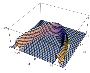
Figure 2: Left, the square of the wave packet $|\Psi(\alpha_{1},\alpha_{2})|^{2}$ for $|\chi_{0}|=12$ and $\theta_{0}=0$, $\omega_{+}=\omega_{-}=1$ with $n_{\mbox{max}}=130$ and right, the contour plot of the same figure with the classical path superimposed as the thick solid line.

that is, the orthonormality and completeness of the basis functions follow from those of the Hermite polynomials. A general wave packet can now be defined as

$$\Psi(\alpha_{1},\alpha_{2})=\Sigma_{n_{1},n_{2}}^{\prime}A_{n_{1},n_{2}}\Phi_{n_{1},n_{2}}(\alpha_{1},\alpha_{2})$$ (85)

where the prime on the sum indicates summing over all values of $n_{1}$ and $n_{2}$ satisfying the constraint (84). The coefficients $A_{n_{1},n_{2}}$ are given by [16]

$$\frac{A_{n_{1},n_{2}}}{\sqrt{2^{n_{2}}n_{2}!}}=\left(\frac{\pi}{\omega_{-}}\right)^{1/4}\frac{(n_{2}/2)!c_{n_{1}}}{(-1)^{n_{2}/2}n_{2}!}$$ (86)

where

$$c_{n}=e^{-1/4|\chi_{0}|^{2}}\frac{\chi_{0}^{n}}{\sqrt{2^{n}n!}}.$$ (87)

The classical paths corresponding to these solutions are the generalized Lissajous ellipsis which have the following parametric representation

$$\alpha_{1}(t)=\alpha_{1}(0)\cos(\omega_{+}t-\theta_{0}),\hskip 14.22636pt\alpha_{2}(t)=\alpha_{2}(0)\sin(\omega_{-}t)$$ (88)

where the zero energy condition demands $\omega_{+}\alpha_{1}(0)=\omega_{-}\alpha_{2}(0)$, and $\theta_{0}$ is an arbitrary phase factor. The classical-quantum correspondence is established by

$$\chi_{0}=\sqrt{\frac{\omega_{+}}{\omega_{-}}}\alpha_{1}(0)e^{i\theta_{0}}.$$ (89)

Figure 2 shows the square of the wave packet $|\Psi(\alpha_{1},\alpha_{2})|^{2}$ for equal frequencies $\omega_{+}=\omega_{-}=1$ and also the corresponding classical path superimposed on it, showing a good classical quantum correspondence. One can also choose the frequencies to be unequal and study the the behavior of the resulting wave packet. An extensive discussion for the construction of wave packets resulting from the solutions of equation (80) with both equal and unequal frequencies can be found in [16].

A final word on these solutions are in order. As the classical solutions corresponding to these wave packets were shown to undergo signature transition, the present quantum cosmological solutions can also be said to have the same behavior in an indirect way.

6 conclusions

In this paper we have considered the analytic expressions for a class of degenerate metric solutions of the Einstein field equations for a self-coupled scalar field in a $(4+d)$-dimensional cosmology with a FRW-type external metric. These solutions depend on a free parameter $\delta$ whose limits are specified by the present observations on the size of the universe. They also predict signature transition from a Euclidean to a Lorentzian domain. For negative eigenvalues of $\Sigma$, we have shown that, within the context of the present work, signature transition can provide a mechanism which would make the scale factors to remain finite. This in turn causes the internal dimension of the model to become stabilized. That is, signature change selects those solutions which are stabilized. The beginning of the Euclidean and ending of the Lorentzian domains are characterized by a singular behavior of the scalar field. Although our exact solutions have been obtained for a spatially flat universe, we predict that the solutions corresponding to $k\neq 0$ will generally show the same type of behavior, as has been shown in [11] for the much simpler case of a $4D$-FRW cosmology. We have also studied the quantum cosmology of our model for the special case when $mm^{\prime}-n=0$ for which the corresponding WD equation was found to have resulted from a Hamiltonian describing an oscillator-ghost-oscillator system. These solutions show a good classical-quantum correspondence in that the classical paths coincide with the crest of the wave functions resulting from the solution of the WD equation.

To conclude, the role of the potential in this and similar models should be duly emphasized. It causes signature transition to occur, stabilizes the internal degrees of freedom and is the vital ingredient for inflation. In turn, signature transition provides a mechanism through which stabilization of, and restriction on the number of internal degrees of freedom can be achieved.
Acknowledgements
The authors would like to thanks S. S. Gousheh and H. Salehi for useful discussions. SJ would like to thank the research council of Shahid Beheshti University for financial support.

References

• [1] K. A. Bronnikov and V. N. Melnikov, Black holes in multi-dimensional dilation gravity: Existance and stability, Ann. phys. 239 (1995) 40
U. Kasper, M. Rainer and A. Zhuk, Integrable multi-component perfect fluid multi-dimensional cosmology II: Scalar fields, Gen. Rel. Grav. 29 (1997) 1123
S. Mignemi and H. schmidt, Classification of multi-dimensional inflationary models, J. Mat. phys. 39 (1998) 998.
• [2] L. Randall and R. Sundrum, An alternative to compactificarion, Phys. Rev. Lett. 83 (1999) 4690
L. Randall and R. Sundrum, A large mass hierarchy from a small extra dimension, Phys. Rev. Lett. 83 (1999) 3370.
• [3] N. Arkani-Hamed, S. Dimopoulos, N. Kaloper and J. March-Russell, Rapid asymmetric inflation and early cosmology in theories with sub-millimeter dimensions, Nucl. Phys. B 567 (2000) 189
D. Lyth, Inflation with Tev-scale gravity, Phys. Lett. B 448 (1999) 191.
• [4] P. S. Wesson, Space-Time-Matter: Modern Kaluza-Klein theory, World Scientific, Singapore, (1999).
• [5] M. Mars, J. M. M. Senovilla and P. Vera, Signature change on the brane, Phys. Rev. Lett. 86 (2001) 4219
D. H. Coule, Does brane cosmology have realistic principles? Class. Quantum Grav. 18 (2001) 4265.
• [6] F. Darabi and H. R. Sepangi, On signature transition and compactification in Kalusa-Klein cosmology, Class. Quantum Grav. 16 (1999) 1565.
• [7] U. Gunther, S. Kriskiv and A. Zhuk, On stable compactification with Casimir-like potential, Grav. Cosmol. 4 (1998) 1.
• [8] U. Gunther and A. Zhuk, A note on dynamical stabilization of internal spaces in multi dimensional cosmology, Class. Quantum Grav. 18 (2001) 1441
A. Mazumdar and A. Perez-Lorenzana, A dynamical stabilization of the radion potential, Phys. Lett. B 508 (2001) 340
U. Blayer and A. Zhuk, Multi-dimensional integrable cosmological models with dynamical and spontaneous compactification [gr-qc/9405028].
• [9] S. M. Caroll, J. Geddes, M. B. Hoffman and R. M. Wald, Classical stabilization of homogeneous extra dimensions, Phys. Rev. D 66 (2002) 024036.
• [10] T. Dereli and R. W. Tuker, Signature dynamics in general relativity, Class. Quantum Grav. 10 (1993) 365.
• [11] K. Ghafoori-Tabrizi, S. S. Gousheh and H. R. Sepangi, On signature transition in Robertson-Walker cosmologies, Int. J. Mod. phys. A 15 (2000) 1521.
• [12] J. P. Mbelek and M. Lachieze-Rey, Theoretical necessity of an external scalar field in the Kaluza-Klein theory, [gr-qc/0012086].
• [13] G. W. Gibbons and Hawking, Action integrals and partition functions in quantum gravity, Phys. Rev. D 15 (1977) 2752
J. W. York, Role of conformal three-geometry in the dynamics of gravitation, Phys. Rev. Lett. 28 (1972)
M. Rainer, The effective sigma-model of multi dimensional gravity, [gr-qc/9812031].
• [14] N. Arkani-Hamed, S. Dimopoulos and G. Dvali, The hierarchy problem and new dimensions at a millimeter, Phys. Lett. B 429 (1998) 263
I. Antoniadis, N. Arkani-Hamed, S. Dimopoulos and G. Dvali, New dimensions at a millimeter to a Fermi and superstring at a Tev, Phys. Lett. B 436 (1998) 257.
• [15] N. Mohammedi, Dynamical compactification, standard cosmology and the accelerating universe, Phys. Rev D 65 (2002) 104018.
• [16] S. S. Gousheh and H. R. Sepangi, Wave packets and initial conditions in quantum cosmology, Phys. Lett. A 272 (2000) 304.