Accuracy estimate for a relativistic Hamiltonian approach to
bound-state problems in theories with asymptotic freedom

Abstract

Accuracy of a relativistic weak-coupling expansion procedure for solving the Hamiltonian bound-state eigenvalue problem in theories with asymptotic freedom is measured using a well-known matrix model. The model is exactly soluble and simple enough to study the method up to sixth order in the expansion. The procedure is found in this case to match the precision of the best available benchmark method of the altered Wegner flow equation, reaching the accuracy of a few percent.

I Introduction

This article describes a foretaste study of accuracy for a recently proposed Hamiltonian weak-coupling expansion procedure that in principle can start from a local asymptotically-free quantum field theory and produce sufficiently small relativistic effective Hamiltonian eigenvalue problems that may be soluble on a computer and yield the wave functions of bound states in that theory. The study is needed to determine the prospects of reaching a reasonable accuracy in the expansion since the strong coupling constant rises when the renormalization group scale is lowered toward the scale of binding mechanism af1 ; af2 . So far, successful approaches required different formulations of the theory at the bound-state and high-energy scales, such as Wilson’s lattice and Feynman’s diagrammatic techniques Wilson:1976kh ; match1 ; match2 ; match3 . They also used approximations such as the non-relativistic limit that applies in the case of heavy quarkonia charm1 ; charm2 ; charm3 ; charm4 and helps in constructing effective theories in analogy with QED CasLep ; krp ; nrqcd1 ; nrqcd2 .

The approach discussed here is the renormalization group procedure for effective particles (RGEP) RGEP that stems from the application of the similarity renormalization group procedure similarity to the light-front Hamiltonian of QCD long . In one and the same scheme, RGEP produces the asymptotically free coupling constant in the Hamiltonians for quarks and gluons g_QCD , provides the conceptual framework for constructing the whole renormalized Poincare algebra in terms of the creation and annihilation operators for effective particles algebra , and leads to a simple first approximation in the case of heavy quarkonia ho . The procedure is boost invariant and raises a hope for connecting the constituent model for hadrons at rest Hagiwara and the parton picture in the infinite momentum frame partons . The key ingredient of the procedure is the vertex form factor $f$ that multiplies all interaction terms. It falls off quickly to zero when the change of an invariant mass in an interaction vertex exceeds the width parameter $\lambda$. This width variable is also the renormalization-group evolution parameter. The effective particles that correspond to a small value of $\lambda$ cannot be copiously created because the form factor makes the interactions effectively weak even if the coupling constant becomes large. The internal structure of the effective particles at such small $\lambda$ may still be given by the parton-like picture in terms of constituents that correspond to a much larger value of $\lambda\sim Q$ in the same flow, where $Q$ is the momentum scale of the external probe largep .

Qualitative accuracy studies of a similarity scheme were performed before modelafbs using the elegant Wegner flow equation Wegner1 ; Wegner2 , which was invented independently for solving Hamiltonian eigenvalue problems in solid state physics. Unfortunately, it was found that the Wegner equation was not suitable for a straightforward weak-coupling expansion beyond second order. The coefficients of the expansion grew too fast and alternated in sign, which lead to erratic results for bound state energies with no signs of convergence. But the Wegner equation can be modified within the similarity scheme optimization and the improved equation provides the benchmark here for estimating the accuracy prospects for the relativistic RGEP procedure. The comparison with the altered Wegner equation and the fact that improvements are also needed in condensed matter physics Mielke1 ; Mielke2 ; Mielke3 , imply that the effective particle approach may also find application outside QCD, i.e., wherever the dynamical couplings increase in the flow of Hamiltonians toward the region of physical interest.

The RGEP strategy that is tested here is to start with a regulated $H$ of the theory to be solved (this $H$ provides an initial condition for the differential equations of RGEP at $\lambda=\infty$), and to evaluate $H_{\lambda}$ with $\lambda$ on the order of a bound-state energy as a series in powers of a coupling constant $g_{\lambda}$. After evaluation of $H_{\lambda}$, one calculates its matrix elements in the basis defined by eigenstates of the Hamiltonian $H_{0\lambda}$, which is obtaind from $H_{\lambda}$ by setting $g_{\lambda}=0$; $H_{0\lambda}|n\rangle=E_{n}|n\rangle$ for all values of the label $n$. Suppose that the labels are ordered so that $E_{m}<E_{n}$ implies $m<n$ and the initial Hamiltonian is regulated by forcing matrix elements $H_{mn}=\langle m|H|n\rangle$ to vanish unless $M\leq m,n\leq N$ with certain ultraviolet cutoff number $N$ and infrared cutoff $M$. The RGEP procedure is designed in such a way that the matrix elements $\langle m|H_{\lambda}|n\rangle$ quickly tend to 0 when $|E_{m}-E_{n}|$ grows above $\lambda$, see Fig. 1. The next step is to focus attention on the window $W_{\lambda}$ of matrix elements of $H_{\lambda}$ among the basis states that have energies similar to the energy scale $E$ of the physical problem at hand, i.e.,

$$W_{\lambda\,mn}=\langle m|H_{\lambda}|n\rangle\,,$$ (1)

with $\tilde{M}\leq m,n\leq\tilde{N}$ and $E_{\tilde{M}}\lesssim E\lesssim E_{\tilde{N}}$. Since only states within the width $\lambda$ on the energy scale can directly interact with each other, states that differ in energy from $E$ by much more than $\lambda$ are usually not important modelafbs ; optimization . They can be important as long as the coupling strength can overcome the difference in energy, but it does not matter here because the coupling constant is assumed to not grow to large values. The next step is to solve the non-perturbative eigenvalue equation for the matrix $W_{\lambda\,mn}$ by diagonalizing it on a computer. The middle-size eigenvalues of $W$ are expected to be close to the exact solutions with accuracy that depends on many factors in the procedure. These dependencies need to be estimated. The main question addressed here concerns the accuracy of the weak-coupling expansion for $W_{\lambda}$.

Figure 1: This out-of-scale figure illustrates Eq. (1) for the matrix $W_{\lambda\,mn}$ with indices $\tilde{M}\leq m,n\leq\tilde{N}$. The matrix of $H_{\lambda}$ is represented by the large square. Matrix elements of $H_{\lambda}$ outside the diagonal band of width $\lambda$ are equivalent to zero. In the model study: $E_{N}\sim 65000$ GeV, $E_{\tilde{N}}\sim 4$ GeV, and the width $\lambda\sim 2$ GeV.

An exact RGEP procedure provides $W_{\lambda\,mn}$ whose structure depends on $\lambda$ but the eigenvalues of the middle size in the window spectrum do not. Becasue the couplings to the states outside the window are ignored, the eigenvalues of sizes at the limits of the window spectrum cannot be accurate even if the window is calculated exactly. Now, when one calculates $W_{\lambda}$ in the expansion in powers of $g_{\lambda}$ to some order, and extrapolates the result to $g_{\lambda}\sim 1$, considerable errors can ensue because of the missing terms in the series. Moreover, one never knows the right value of $g_{\lambda}$ at given $\lambda$ from the theory. Therefore, one must fit $g_{\lambda}$ to the bound-state observables and perform consistency checks for a whole set of them. The smaller is $\lambda$ the larger is $g_{\lambda}$ and the more significant are the errors of perturbation theory in evaluation of $W_{\lambda}$. But at the same time the larger is $\lambda$, the larger must be the range $[\tilde{M},\tilde{N}]$ of basis states needed in the computer diagonalization of $W_{\lambda}$. A compromise must be made and the critical question is how close one can come to a true solution using RGEP equations. The question is essential for the prospects of applying RGEP to QCD. A well-known asymptotically free matrix model is used here to find out what level of accuracy can in principle be expected. One should stress at this point that even if the test gave a promising result in the model, the utility of the procedure would remain only tentative until the actual calculations in realistic theories are performed and display signs of stability as functions of the order of the expansion, size of $\lambda$, variation of the window, and other more specific features of the eigenvalue problems at hand.

Section II defines the test model and quotes equations used for calculating $H_{\lambda}$ in the benchmark of the altered Wegner’s flow and in the RGEP case. Section III describes results obtained using six different ways of fitting the coupling constant to the exact spectrum. These ways are labeled throughout the paper by letters A, B, C, D, E, and F. Each of these versions is studied in six successive orders of the weak-coupling expansion. Section IV provides a brief conclusion. Appendix A contains the generic analytic RGEP formula for 4th order calculations that applies to arbitrary $H$, and Appendix B provides the numbers that illustrate in detail what happens in the expansions including from one to six orders.

II Model

The matrix elements of the model Hamiltonian used here for estimating the accuracy of RGEP are modelafbs ; optimization

$$H_{mn}\,=\,E_{n}\,\delta_{mn}\,-\,g\,\sqrt{E_{m}E_{n}}\,,$$ (2)

where $E_{n}=b^{n}$, $b>1$, and $n$ is an integer, with a convention that the energy equal 1 corresponds to 1 GeV. The model diverges and needs to be regulated by the ultraviolet cutoff $\Lambda=b^{N}$ that limits the allowed energies $E_{n}$ from above. Also a low energy cutoff, $b^{M}$, is introduced for making the Hamiltonian matrix finite and enable exact computations, but the lower bound is of no physical consequence for the results reported here. Thus, the subscripts in Eq. (2) are limited to the range $[M,N]$, $M$ being large negative and $N$ large positive. The ultraviolet renormalizability of the model, its asymptotic freedom, and its lack of sensitivity to the infrared cutoff, were described in modelafbs ; optimization .

Two values of the cutoff $N$ and the corresponding coupling constant $g=g_{N}$ are used in this study of RGEP: $g_{16}=0.060600631$ and $g_{20}=0.04878048667$. The two cutoffs are introduced to verify the accuracy of renormalizability in the RGEP scheme. It is known that for such large values of $N$ the effective dynamics with $\lambda\sim 1$ is practically independent of $N$ in the case of altered Wegner’s equation, and one can verify how well the RGEP approach satisfies this condition. At the same time, this condition puts constraints on the range of changes that one can consider in varying the RGEP generator without interference with renormalizability (see below). The coupling constants $g_{16}$ amd $g_{20}$ are fitted to obtain the exact bound-state eigenvalue $E=-1$ with 8 digits of accuracy for $b=2$ and $M=-21$, as in optimization . With these choices, the Hamiltonian $H$ is a $(N-M+1)$ $\times$ $(N-M+1)$ matrix with $N-M$ positive eigenvalues, and one negative, spanning the range of energies between $E_{M}\sim 0.5$ KeV and $E_{N}\sim 65$ or 1000 TeV.

The similarity renormalization group procedure for Hamiltonians that leads to the altered Wegner equation Wegner1 ; optimization and provides the benchmark here, can be written in the differentail form as

$$\frac{d\mathcal{H}}{d\lambda}=\left[F\{\mathcal{H}\},\mathcal{H}\right]\,,$$ (3)

with the initial condition $\mathcal{H}=H$ when $\lambda=\infty$. The initial condition contains counterterms but the similarity analysis showed similarity that the structure of the counterterms is simple and the presence of them is equivalent for large $N$ to making $g$ in $H$ depend on $N$. This is precisely what is done by the fitting mentioned earlier that guarantees that the eigenvalue $E=-1$ stays unchanged for different $N$s. All small eigenvalues are then independent of $N$. The generator of the similarity transformation can be written as ($\mathcal{D}_{m}=\mathcal{H}_{mm}$)

$$\langle m|F\{\mathcal{H}\}|n\rangle=h_{mn}(\mathcal{D}_{m}-\mathcal{D}_{n})\mathcal{H}_{mn}\,.$$ (4)

Different choices of $h_{mn}$ lead to different matrix elements of the renormalized Hamiltonians. Assuming

$$h_{mn}=\phi_{mn}\,{ds\over d\lambda}\,,$$ (5)

one obtains Wegner’s equation when $\phi_{mn}\equiv 1$, and $s=1/\lambda^{2}$ plays the role of the original Wegner parameter l Wegner1 . The altered Wegner equation has optimization

$$\phi_{mn}={1\over 1+|m-n|}\,,$$ (6)

and this new equation is referred to as the benchmark.

In the plain perturbative RGEP procedure, the matrix elements of $H_{\lambda}$ in the effective basis states associated with the scale $\lambda$, are obtained from the matrix elements of an auxiliary Hamiltonian $\mathcal{H}$ in the initial basis RGEP . The structure of $\mathcal{H}$ is given by

$$\mathcal{H}\,=\,\mathcal{H}_{0}\,+\,f\mathcal{G}_{I}\,.$$ (7)

The Hamiltonian $\mathcal{H}_{0}$ is equal to the initial $H_{0}$, which is the free part of $H$, i.e., $H$ with $g=0$. $f$ denotes the form factor that can be written in all matrix elements using eigenvalues of $\mathcal{H}_{0}$, and reads

$$f_{mn}=\exp{\left[-\,\phi_{mn}\,\frac{(E_{m}-E_{n})^{2}}{\lambda^{2}}\right]}\,.$$ (8)

The RGEP equation for $\mathcal{G}_{I}$ is

$$\frac{d\mathcal{G}_{I}}{d\lambda}=\left[f\mathcal{G}_{I},\,\left\{{d\over d\lambda}\,(1-f)\mathcal{G}_{I}\right\}\right]\,,$$ (9)

where the curly bracket around an operator has the following meaning in terms of the matrix elements,

$$\left\{A\right\}_{mn}=\frac{A_{mn}}{E_{n}-E_{m}}\,.$$ (10)

A priori, the optimal choice for $\phi_{mn}$ in the RGEP could be different from the one that optimized the benchmark optimization . But we have studied various factors $\phi_{mn}$ a la optimization and found that $c\sim 1$ is also the best choice to make in RGEP, for similar reasons. In addition, it is useful for the test that these factors are made equal since then the first order calculations give identical results in both approaches. The factor $\phi_{mn}$ is included in the analytic 4th order RGEP formulae provided in Appendix A.

The RGEP Eq. (9) cannot be integrated exactly on a computer as easily as Wegner’s equation can, because it contains the derivative of $\mathcal{G}_{I}$ on its right-hand side. One has to solve a complex linear problem to extract ${\mathcal{G}}^{\prime}_{I}$. But the altered Wegner equation provides a perturbative benchmark pattern that is known to approximate an exact solution well and one can estimate the accuracy of RGEP by comparison.

In the perturbative evaluation of $H_{\lambda}$, the RGEP calculus is free from the problem of extracting ${\mathcal{G}}^{\prime}_{I}$ because the derivative is computed order by order and all terms needed on the right-hand side are known at each successive order from the lower order results. In fact, the new procedure is designed for a perturbative approach. It is simpler than the Wegner case in the sense that the form factors guarantee the band structure in perturbation theory so that this structure does not have to be recovered from and controlled in the evolution of specific matrix elements. Small energy denominators that might otherwise lead to infrared singularities are excluded by design of RGEP. It also does not generate any terms with inverse powers of $\lambda$ in the coefficients of products of the interaction Hamiltonian (see Appendix A and Eq. (3.2) in optimization ). Such terms can in principle lead to a variety of mixing effects in the evolution of $H_{\lambda}$, when one uses the Wegner equation. On top of these purely quantum mechanical features, the perturbative RGEP calculus is capable of respecting seven Poincare symmetries in an economic way and has a potential to obtain the remaining three algebra . At the same time, it preserves the cluster decomposition property Weinberg in the effective interactions. All these features are desired for the description of relativistic particles using theories with asymptotic freedom. But the accuracy of the weak-coupling expansion for windows $W_{\lambda}$ in RGEP must be measured against the benchmark to estimate the cost of the apparent advantages in terms of precision.

III Accuracy of RGEP

The results of weak-coupling expansions up to the first-order terms in the RGEP and altered Wegner equation are identical, and read

$$\mathcal{H}_{mn} = E_{m}\delta_{mn}-g_{\lambda}\,\sqrt{E_{m}E_{n}}\,f_{mn}\,.$$ (11)

The form factor $f_{mn}$ causes that the interaction Hamiltonian matrix is narrow on the energy scale and has width $\lambda$, see Figure 1. It is clear that in the case of Eq. (11) the effective coupling constant can be extracted from the matrix $\mathcal{H}$ using the formula

$$g_{\lambda}=1-\frac{\mathcal{H}_{M,M}(\lambda)}{E_{M}}\,,$$ (12)

which is analogous to the Thomson limit in QED when $M$ is large and negative. The same Eq. (12) is used for defining $g_{\lambda}$ also in higher order calculations.

In the weak-coupling expansion in powers of $g_{\lambda}$ to order $k$ (see e.g. optimization ),

$$\mathcal{H}=\mathcal{H}_{0}+g_{\lambda}\mathcal{H}_{1}+g_{\lambda}^{2}\mathcal{H}_{2}+...+g_{\lambda}^{k}\mathcal{H}_{k}\,.$$ (13)

Appendix A contains analytic expressions for $\mathcal{H}_{k}$ with $k=1$, 2, 3, and 4. The right value of $g_{\lambda}$ can be found by solving the flow equations with the initial condition $g_{\infty}=g_{N}$ exactly. Then, one can check the accuracy of a perturbatively computed $H_{\lambda}$ by diagonalizing it for the exact value of $g_{\lambda}$, and by comparing the resulting bound-state eigenvalue with $E=-1$ that was secured to exist by the initial choice of $g_{N}$ modelafbs ; optimization . The accuracy test for RGEP is carried out differently because the exact solution of Eq. (9) is not known. This situation is analogous to QCD where one can use perturbation theory to calculate $H_{\lambda}$ but an exact value of $g_{\lambda}$ is not available as a function of $g_{N}$. For the purpose of the accuracy test, the exact spectrum of the model is treated as experimental data. An approximate value of $g_{\lambda}$ is found by fitting some eigenvalue of the perturbatively calculated $W_{\lambda}$ to the data, or by performing a fit for a whole group of eigenvalues. Then one checks how well the bound-state eigenvalue $E=-1$ is reproduced using the best-fit value for $g_{\lambda}$. In principle, one could fit $g_{\lambda}$ at one value of $\lambda$ that is most convenient for that purpose, evolve this value using RGEP to the new $\lambda$ that is most suitable for the bound-state calculation, and then compare the calculated spectrum with data g1 ; match3 ; g2 ; g3 . In fact, the model used here can be used for testing accuracy of such procedures in a comprehensive way. This type of tests may help in narrowing the current spread of estimates for $\alpha_{s}$ that come from various sources Hagiwara , by distinguishing theoretical procedures of least ambiguity. But the accuracy of RGEP is checked here using one and the same scale for fitting $g_{\lambda}$ and calculating the bound-state energy, for simplicity. The scale we choose is $\lambda=2$.

There exist infinitely many options for how one can fit $g_{\lambda}$ so that the spectrum of the window $W_{\lambda}$ at $\lambda=2$ approximates the exact one as closely as possible. We display results for six options that illustrate the dependence of results on such choices, labeled by A, B, C, D, E, and F. All methods are based on the minimalization of certain function $K(g_{\lambda})$. We use

$$K_{r}(g_{\lambda})=Z\sum_{n}\left(\frac{v_{n}}{v_{e\,n}}-1\right)^{2}\,,$$ (14)

and

$$K_{s}(g_{\lambda})=Z\sum_{n}\left(\frac{v_{n}-v_{n+1}}{v_{e\,n}-v_{e\,n+1}}-1\right)^{2}\,,$$ (15)

where $v_{e\,n}$ is the exact eigenvalue of number $n$, and $v_{n}$ is the corresponding eigenvalue of $W_{\lambda}$ when $W_{\lambda}$ is derived in a given order $k$. $Z$ is the normalization constant equal to the inverse of the number of terms in the sum. $Z$ is not important in the minimalization of $K(g_{\lambda})$ as function of $g_{\lambda}$. The subscript $r$ refers to the ratios of eigenvalues used in $K_{r}$, and the subscript $s$ refers to the splittings between the eigenvalues used in $K_{s}$. The six choices differ by which function $K(g_{\lambda})$ is used and what is the range of summation over $n$ in Eqs. (14) or (15).

The eigenvalues of $H$ are numbered from $M$ to $N$ in the order in which they appear on the diagonal of $H_{\lambda}$ when $\lambda\rightarrow 0$ in the benchmark calculation. This numbering is also applied to the corresponding rows and columns of the matrix $H_{\lambda\,mn}$. The window $W_{\lambda}$ is always chosen to extend from $\tilde{M}=-8$ to $\tilde{N}=2$ optimization , and it has 11 eigenvalues. These are numbered in the same order as for $H_{\lambda}$, with the bound-state eigenvalue having number $n_{0}$. We distinguish two eigenvalues that are closest in modulus to the bound-state energy $E=-1$, one just smaller than 1, with number $n_{s}$, and one just larger than 1 with number $n_{l}$. The six fitting procedures are designated as follows:

$${\rm A} \Rightarrow K_{r},\,n=n_{s}\,,$$ (16)

$${\rm B} \Rightarrow K_{r},\,n=n_{l}\,,$$ (17)

$${\rm C} \Rightarrow K_{r},\,n\in\{n_{s},n_{l}\}\,,$$ (18)

$${\rm D} \Rightarrow K_{s},\,n=n_{l}\,,$$ (19)

$${\rm E} \Rightarrow K_{r},\,n\in[\tilde{M}+2,\tilde{N}-2]\,,n\neq n_{0}\,,$$ (20)

$${\rm F} \Rightarrow K_{s},\,n\in[\tilde{M}+2,\tilde{N}-2]\,,n\neq n_{0}\,.$$ (21)

In cases E and F, the two smallest and two largest eigenvalues are dropped because they are too much distorted by the edge of $W_{\lambda}$, as explained in Section I. The description of results obtained in the benchmark and tested approach in six successive orders of perturbation theory in each of these fitting schemes involves 72 results. The benchmark results are labeled ”Wegner” and the tested case is labeled ”RGEP.” Appendix B contains all pertinent numbers. An example is given below to help in reading the figures and tables in the appendix. Otherwise, only main features of the results are explained.

Fig. 2 corresponds to the case C of Eq. (18). The shape of $K(g_{\lambda})$ clearly selects the value of $g_{\lambda}$ preferred by a given fitting procedure. Similar plots in other cases are given in Fig. 6 in Appendix B. The numbers that result from the fits for the coupling constants, along with the corresponding bound-state eigenvalues of $W_{\lambda}$, are also tabulated in Appendix B.

The summary of results for the coupling constants obtained in the fits is given in Fig. 3. The numbers 1 to 6 on the horizontal axis correspond to the order of perturbation theory in the evaluation of $W_{\lambda}$. The columns labeled A to F correspond to the algorithms given in Eqs. (16) to (21). The RGEP calculation equals the benchmark in the first order results. It is also visible that the fits of $g_{\lambda}$ in the benchmark case consistently reproduce the exact value of $g_{\lambda}=0.2852$ at $\lambda=2$ GeV optimization . The RGEP

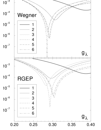
Figure 2: Plots of $K(g_{\lambda})$ from Eq. (14), in the altered Wegner case (benchmark), and in the RGEP procedure, as marked, in the fit C of Eq. (18) and six successive orders of perturbation theory used in evaluation of the window $W_{\lambda}$, with the renormalization group parameter $\lambda=2$ GeV, as functions of the a priori unknown value of the coupling constant $g_{\lambda}$ at this $\lambda$. $K(g_{\lambda})$ measures deviation of two selected eigenvalues of the window $W_{\lambda}$ (those which are nearst-in-size to the bound-state eigenvalue) from their exact counterparts. The shapes of the functions point toward the required values of $g_{\lambda}$. This example is provided for explanation of how to read other examples given in Appendix B.

displays similar stability and coalesces around 0.3. However, when the nearst neighbor level with energy larger than 1 is included in a fit as the only one (case B), or together with a nearest lower level using ratios of eigenvalues (case C), or together with the nearest lower level but using ratios of splittings between the two eigenvalues (case D), a visible variation in the fits occurs. This variation can be attributed to the lack of accuracy in the calculation of the nearst higher level, since in the cases E and F that include additional five lower levels, the higher level becoming much less significant, the fits resemble case A where the higher level is absent. This result suggests a rule for fits in future calculations that they should be focused on states with eigenvalues as far as possible from the bounds implied by the window choice and $\lambda$, in order to avoid the lack of convergence. Note that even in the benchmark case the 4th order calculation has to be corrected in the orders 5th and 6th to bring the accuracy into the few percent range around the exact value of $g_{\lambda}$. The same effect is observed in the bound-state eigenvalues themselves.

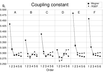
Figure 3: Coupling constants $g_{\lambda}$ obtained from fits described in Eqs. (16) to (21), gathered in the columns labeled by A to F, in the benchmark case (Wegner) and the tested case (RGEP). The six entries in each column correspond to six successive orders of perturbation theory used in the calculation of the window $W_{\lambda}$ with $\lambda=2$ GeV.

The summary of results for the bound-state eigenvalues is provided in Fig. 4 in a one-to-one correspondence to Fig. 3. The eigenvalues are obtained by diagonalization of windows $W_{\lambda}$ that are calculated in the six consecutive orders of perturbation theory (indicated on the horizontal axis in the individual columns), using the corresponding values of $g_{\lambda}$ from Fig. 3 (the numbers are given in Appendix B). It is visible that the RGEP procedure matches accuracy of the altered Wegner equation. One also sees the dramatic effect of the attempts to include the next higher level. The results clearly point out that both procedures should not be used for calculations of energy levels close to the size of $\lambda$. The fourth order calculations achieve accuracy on the order of 5%. This is encouraging, because orders 5 and 6 lead to even better results and one can expect that fits for $g_{\lambda}$ can be improved by focusing on the properties of low energy levels, including properties other than just eigenvalues. It is hard to imagine that such focus could lead to worsening of the accuracy.

Figure 4: Energies of bound states obtained from a non-perturbative diagonalization of window matrices $W_{\lambda}$ with $\lambda=2$ GeV. The matrices were derived in perturbation theory and evaluated using the corresponding values of the renormalized coupling constants, $g_{\lambda}$, from Fig. 3. The eigenvalues are displayed in the same convention and in the one-to-one correspondence to Fig. 3. Numerical values are tabulated in Appendix B. The exact result is -1.

The last question concerning accuracy of the RGEP method concerns renormalizability, which can be studied in analogy to optimization . However, one has to measure the sensitivity of the effective theory at the scale $\lambda$ to the cutoff $\Lambda=b^{N}$ in a whole range of coupling constants, because the exact value of $g_{\lambda}$ is not known in the RGEP procedure. Using $g_{16}$ and $g_{20}$ from Section II, we calculate $W_{\lambda}$ starting from $H$ with the two different values of $\Lambda$ for $N=16$ and $N=20$, and we compare the resulting matrix elements of $W_{\lambda}$ at $\lambda=2$ GeV. For $b=2$ the cutoff is changed by the factor 16, i.e. from about 65 TeV to about 1000 TeV. The divergence in the bare theory is logarithmic. The results could change at the rates implied by the change in the logarithm of $\Lambda$, i.e., about 25%, but in the presence of a proper set of counterterms similarity one expects no change to occur. Fig. 5 shows the measure of changes in $W_{\lambda}$ that are obtained here with only one counterterm, which amounts to the change of the coupling constant from $g_{16}$ to $g_{20}$. The function plotted in 5 is defined as

$$R(g_{\lambda})=\sum_{n,m=\tilde{M}}^{\tilde{N}}\left[\,\frac{W_{\lambda\,mn}(N=16)}{W_{\lambda\,mn}(N=20)}\,-\,1\,\right]^{2}\,.$$ (22)

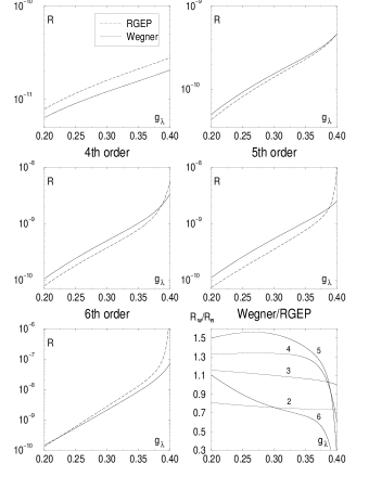
Figure 5: Plots of the renormalizability measure $R(g_{\lambda})$ from Eq. (22) for the RGEP procedure (dashed lines) and the altered Wegner equation (solid line). The last diagram displays the ratios $R_{W}/R_{R}$ (with $R_{W}$ standing for the benchmark $R$, and $R_{R}$ for the $R$ in the RGEP procedure), and the integer labels indicate the corresponding orders of the weak-coupling expansion.

The results change with the order of perturbation theory used for evaluation of $W_{\lambda}$. The sensitivity of results to the change of $\Lambda$ in 1st order is the same in RGEP as in the benchmark case optimization . Inclusion of higher orders, from 2 to 6, exhibits slight variations to the advantage of one or the other method, as shown in Fig. 5 (the solid line for the benchmark and the dashed one for RGEP). The last diagram in Fig. 5 shows the corresponding ratio $R_{W}/R_{R}$, and it demonstrates that the renormalizability condition is satisfied with the same accuracy in both approaches. A closer comparison requires that the benchmark case (or $R_{W}$) is taken for $g_{\lambda}=0.2852$, and RGEP (or $R_{R}$) for some $g_{\lambda}\sim 0.3\pm 0.005$ (see Appendix B), but these corrections are negligible at the current stage of the analysis.

IV Conclusion

The RGEP weak-coupling expansion achieves precision comparable with that of the best available benchmark method of the altered Wegner equation in the case of a simple matrix model for the Hamiltonian formulation of theories with asymptotic freedom and bound states. The few percent accuracy is reached by introducing a factor of $\phi$ in Eq. (6), which is similar in both methods. Since the RGEP procedure is designed for application to relativistic quantum field theory, the model test calculation provides a comprehensive outline of steps that can be repeated in realistic cases, especially in the theory of quarks and gluons. On the other hand, knowing that Wegner’s equation is useful in condensed matter physics, one can expect that the altered Wegner equation and the RGEP procedure may also find applications in many-body theory. The model study indicates a possibility that the weak-coupling expansion may lead to a systematic approximation scheme despite the growth of the coupling when the characteristic scale $\lambda$ of the effective theories is lowered. This is indicated in columns E and F in Figs. 3 and 4, where one can see the convergence of the coupling constant to a stable value and the corresponding convergence of the bound-state energy to the exact result. One should also note that already second order calculations render effective window Hamiltonians $W_{\lambda}$ that can produce the bound-state eigenvalue with accuracy better than 10%.

The fact that both methods have similar accuracy suggests that they already show the range of calculational power that is available through a plain expansion in a single coupling constant such as the one defined in Eq. (12). In order to move beyond the 1% accuracy level one has to achieve better understanding of the structure of $H_{\lambda}$. For example, there exist terms in $H_{\lambda}$ with specific dependence on the eigenvalues of $H_{0}$ and $\lambda$, like $(E_{m}-E_{n})^{2}/\lambda^{2}$ in the model. One may hope to understand how the coefficients of these terms depend on a more suitably defined coupling constant than the one given Eq. (12). It is conceivable that such understanding may further improve the weak-coupling expansion. Note also that none of the renormalization group universality features were so far explicitly employed in the plain expansion tested here. Such options for improvement may depend on a theory. One has to study specific theories using concrete versions of the RGEP procedure in order to identify the dominant terms and their universal behavior.

The accuracy study for the RGEP procedure shows also that one should be able to carry out similar tests for any other approach to the bound-state problem in asymptotically free theories. For such a test to become possible, the approach in question would have to be understood sufficiently well to determine the steps that that approach implies for handling of the initial $H$ in the model. But such understanding is demanded of most formulations of relativistic quantum theories for fundamental reasons and the accuracy tests of similar kind can be consider a challenge for any scheme intended to solve the bound-state problem in theories with asymptotic freedom.

Appendix A RGEP of 4th order

The RGEP weak-coupling expansion for terms of order $g^{n}$, is written using terms of orders $k<n$,

$$\mathcal{G}_{n}^{{}^{\prime}} = \sum_{k=1}^{n-1}\left[f\mathcal{G}_{k},\left\{\left(1-f\right)\mathcal{G}_{n-k}\right\}^{{}^{\prime}}\right]\,.$$ (23)

If the interaction Hamiltonian $H_{I}=H-H_{0}$ is proportional to $g$, the expansion in powers of $g$ is the same as the expansion in powers of $H_{I}$. If $H_{I}$ contains a polynomial in $g$ with operator coefficients, then the expansion in powers of $H_{I}$ is an intermediate step for obtaining an expansion for $H_{\lambda}$ in powers of $g$. Therefore, this appendix provides a generic set of coefficients for expansion of $\mathcal{G}_{k}(\lambda)$ in powers of $H_{I}$. The argument $\lambda$ is omitted in what follows. The procedure of rewriting the expansion in powers of the bare $g$ into the expansion in powers of $g_{\lambda}$ requires a definition of $g_{\lambda}$ in the structure of $H_{\lambda}$. This definition, in analogy to Eq. (12), provides then a series expression for $g_{\lambda}(g)$. This expression is inverted and substituted into the formal expansion of $H_{\lambda}$ in powers of the bare $g$, producing the desired expansion in powers of $g_{\lambda}$.

The first four terms in the perturbative expansion are written as

$$\left[\mathcal{G}_{1}\right]_{mn} = H_{mn}\,,$$ (24)

$$\left[\mathcal{G}_{2}\right]_{mn} = a_{m1n}H_{m1}H_{1n}\,,$$ (25)

$$\left[\mathcal{G}_{3}\right]_{mn} = b_{m12n}H_{m1}H_{12}H_{2n}\,,$$ (26)

$$\left[\mathcal{G}_{4}\right]_{mn} = c_{m123n}H_{m1}H_{12}H_{23}H_{3n}\,.$$ (27)

It is uderstood that the indices 1, 2, and 3, are summed over the entire range available for them in the theory.

In order to write down expressions for the coefficients $a$, $b$, and $c$, we introduce a set of auxiliary symbols. Their meaning becomes sucessively self-evident when one decifers them in the order they are given here. The variables $s$ and $t$ have the meaning of the renormalization group parameter $1/\lambda^{2}$.

$$E_{mn} = E_{m}-E_{n}\,,$$ (28)

$$G_{mn} = \varphi_{mn}\left(E_{m}-E_{n}\right)\,,$$ (29)

$$F_{mn} = \varphi_{mn}\left(E_{m}-E_{n}\right)^{2}\,,$$ (30)

$$G_{m1n} = G_{1m}+G_{1n}\,,$$ (31)

$$F_{m...lkn} = F_{m...lk}+F_{kn}\,,$$ (32)

$$A_{ml...kn}(t) = f_{ml}...f_{kn}\,,$$ (33)

$$A_{m...l+k...n}(t) = A_{m...l}(t)\,A_{k...n}(t)\,,$$ (34)

$$B_{m...k}(s) = \int_{0}^{s}dtA_{m...k}(t)\,.$$ (35)

In this notation one obtains

$$a_{m1n} =G_{m1n}\, B_{m1n}\,.$$ (36)

$$b_{m12n} = \frac{G_{m12}}{E_{m2}}\left[B_{m12n+m2}-B_{m12n}\right]$$ (37)

$$+ \frac{G_{n12}}{E_{n2}}\left[B_{m21n+n2}-B_{m21n}\right]$$

$$+ \frac{G_{m1n}\,G_{m12}}{F_{m12}}\left[B_{m2n+m12}-B_{m2n}\right]$$

$$+ \frac{G_{m1n}\,G_{n12}}{F_{n12}}\left[B_{m2n+n12}-B_{m2n}\right]$$

$$c_{m123n} = \frac{G_{23m}}{E_{m1}\,E_{m2}}\left[B_{m321n}-B_{m321n+1m}-B_{m321n+2m}+B_{m321n+1m2}\right]$$ (38)

$$+ \frac{G_{23n}}{E_{n1}\,E_{n2}}\left[B_{m123n}-B_{m123n+1n}-B_{m123n+2n}+B_{m123n+1n2}\right]$$

$$+ \frac{G_{132}}{E_{12}\,E_{m1}}\left[B_{m231n}-B_{m231n+21}-B_{m231n+m1}+B_{m231n+m12}\right]$$

$$+ \frac{G_{132}}{E_{12}\,E_{n1}}\left[B_{m132n}-B_{m132n+21}-B_{m132n+n1}+B_{m132n+n12}\right]$$

$$+ \frac{G_{12m}\,G_{23m}}{F_{23m}\,E_{m1}}\left[B_{m21n}-B_{m21n+m1}-B_{m21n+m32}+B_{m21n+1m32}\right]$$

$$+ \frac{G_{12n}\,G_{23n}}{F_{23n}\,E_{n1}}\left[B_{m12n}-B_{m12n+n1}-B_{m12n+n32}+B_{m12n+1n32}\right]$$

$$+ \frac{G_{12m}\,G_{13n}}{F_{13n}\,E_{m1}}\left[B_{m21n}-B_{m21n+m1}-B_{m21n+n31}+B_{m21n+m13n}\right]$$

$$+ \frac{G_{12n}\,G_{13m}}{F_{13m}\,E_{n1}}\left[B_{m12n}-B_{m12n+n1}-B_{m12n+m31}+B_{m12n+m31n}\right]$$

$$+ \frac{G_{12m}\,G_{132}}{F_{132}\,E_{m1}}\left[B_{m21n}-B_{m21n+m1}-B_{m21n+132}+B_{m21n+m132}\right]$$

$$+ \frac{G_{12n}\,G_{132}}{F_{132}\,E_{n1}}\left[B_{m12n}-B_{m12n+n1}-B_{m12n+132}+B_{m12n+n132}\right]$$

$$+ \frac{G_{m1n}\,G_{23m}}{E_{m2}}\left[\frac{B_{m1n}-B_{m1n+m321}}{F_{m321}}-\frac{B_{m1n}-B_{m1n+m321+m2}}{F_{m321}+F_{2m}}\right]$$

$$+ \frac{G_{m1n}\,G_{23n}}{E_{n2}}\left[\frac{B_{m1n}-B_{m1n+n321}}{F_{n321}}-\frac{B_{m1n}-B_{m1n+n321+n2}}{F_{n321}+F_{2n}}\right]$$

$$+ \frac{G_{m1n}\,G_{132}}{E_{12}}\left[\frac{B_{m1n}-B_{m1n+m231}}{F_{m231}}-\frac{B_{m1n}-B_{m1n+m2132}}{F_{m231}+F_{21}}\right]$$

$$+ \frac{G_{m1n}\,G_{132}}{E_{12}}\left[\frac{B_{m1n}-B_{m1n+n231}}{F_{n231}}-\frac{B_{m1n}-B_{m1n+n2132}}{F_{n231}+F_{21}}\right]$$

$$+ \frac{G_{m1n}\,G_{12m}\,G_{23m}}{F_{23m}}\left[\frac{B_{m1n}-B_{m1n+m21}}{F_{m21}}-\frac{B_{m1n}-B_{m1n+m321+m2}}{F_{m21}+F_{m32}}\right]$$

$$+ \frac{G_{m1n}\,G_{12n}\,G_{23n}\,}{F_{23n}}\left[\frac{B_{m1n}-B_{m1n+n21}}{F_{n21}}-\frac{B_{m1n}-B_{m1n+n321+n2}}{F_{n21}+F_{n32}}\right]$$

$$+ \frac{G_{m1n}\,G_{12m}\,G_{132}}{F_{132}}\left[\frac{B_{m1n}-B_{m1n+m21}}{F_{m21}}-\frac{B_{m1n}-B_{m1n+m2312}}{F_{m21}+F_{231}}\right]$$

$$+ \frac{G_{m1n}\,G_{12n}\,G_{132}\,}{F_{132}}\left[\frac{B_{m1n}-B_{m1n+n21}}{F_{n21}}-\frac{B_{m1n}-B_{m1n+n2312}}{F_{n21}+F_{231}}\right]$$

$$+ \frac{G_{m1n}\,G_{12n}\,G_{13m}}{F_{12n}\,F_{13m}}\left[B_{m1n}-B_{m1n+n21}-B_{m1n+m31}+B_{m1n+m312n}\right]$$

In relativistic applications, these formulae need a replacement of the differences of energies like $E_{m}-E_{n}$ by the changes of invariant masses in the interaction vertices, and multiplication of $G_{mn}$ by the parent momenta $P^{+}_{mn}$ in the vertices, see e.g. g_QCD ; ho .

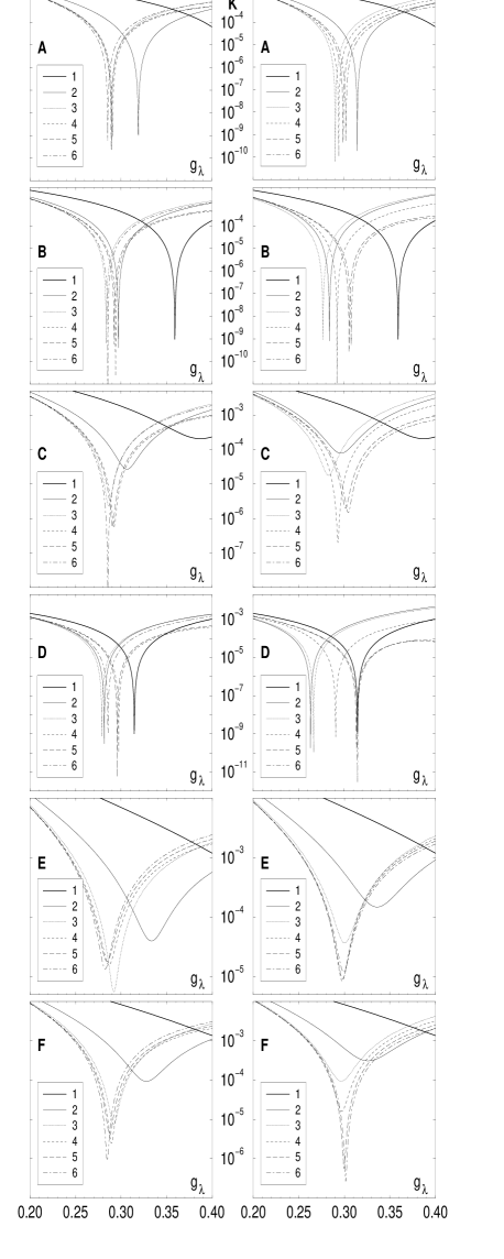
Figure 6: The functions $K(g_{\lambda})$ from Eqs. (16) to (21) plotted for Wegner and RGEP cases, $\lambda=2$ GeV. In all cases a preferred value of $g_{\lambda}$ is clearly identified. These are given in Table I.

	Wegner		RGEP
$k$	$g_{\lambda}$	$|E_{k}|$	$g_{\lambda}$	$|E_{k}|$
A
1	0.43340	0.830955	0.43340	0.830955
2	0.31900	0.984874	0.31460	0.826301
3	0.28985	1.006771	0.29040	0.864725
4	0.29095	1.045453	0.29370	0.911430
5	0.28930	1.032121	0.29865	0.958206
6	0.28545	1.005530	0.30195	0.987875
B
1	0.35915	0.539380	0.35915	0.539380
2	0.29700	0.807142	0.28380	0.619971
3	0.28380	0.943143	0.27665	0.746829
4	0.29425	1.082537	0.29205	0.896377
5	0.29260	1.069262	0.30525	1.020620
6	0.28545	1.005530	0.29205	0.896377
C
1	0.38720	0.644935	0.38720	0.644935
2	0.30690	0.885308	0.29645	0.701781
3	0.28655	0.971815	0.28270	0.797715
4	0.29260	1.063916	0.29315	0.906400
5	0.29095	1.050609	0.30140	0.984000
6	0.28545	1.005530	0.30415	1.008693
D
1	0.31460	0.385414	0.31460	0.385414
2	0.28160	0.691679	0.26290	0.494306
3	0.27885	0.892589	0.26620	0.662643
4	0.29755	1.120255	0.29040	0.881438
5	0.29590	1.107059	0.31350	1.101064
6	0.28545	1.005530	0.31460	1.110135
E
1	0.48345	1.046788	0.48345	1.046788
2	0.33330	1.108054	0.33605	0.983708
3	0.29205	1.030408	0.30030	0.954532
4	0.28655	0.996998	0.29755	0.946995
5	0.28435	0.977641	0.29810	0.953083
6	0.28270	0.974623	0.29920	0.962119
F
1	0.45760	0.933635	0.45760	0.933635
2	0.32780	1.059985	0.32615	0.909722
3	0.29205	1.030408	0.29645	0.919122
4	0.28930	1.027150	0.29700	0.941877
5	0.28765	1.013796	0.29975	0.968487
6	0.28490	0.999307	0.30140	0.982700

Table 1: The values of the couplings $g_{\lambda}$, which correspond to the minima of curves in Fig. 6 (the last digit is given with error margin of 5), and the corresponding results (obtained with the coupling constants given in this table) for the bound state energy $|E_{k}|$ (the exact value is 1), obtained by diagonalization of $W_{\lambda}$ with $\lambda=2$ GeV, that was calculated in six successive orders of the weak-coupling expansion, $k$.

Appendix B Numerical details

Numerical integration of Eqs. (3) and (9) was performed using fourth-order Runge-Kutta procedure and an automated algorithm for generating expressions of order $n$ from expressions of orders $k<n$. The numerically calculated matrix elements $H_{\lambda\,mn}$ were checked using analytic formula from Appendix A.

The fits of the coupling constants $g_{\lambda}$ that were used in the perturbative evaluation of the windows $W_{\lambda}$, were obtained using the functions $K(g_{\lambda})$ from Eqs. (14) and (15) that are plotted in Fig. 6. The corresponding numbers for the coupling constants are given in Table I.

References

- (1) D. J. Gross, F. Wilczek, Phys. Rev. Lett. 30, 1343 (1973).
- (2) H. D. Politzer, Phys. Rev. Lett. 30, 1346 (1973).
- (3) K. G. Wilson, in New pathways in high-energy physics, Orbis Scientiae, 1976.
- (4) A. Hasenfratz, P. Hasenfratz, Phys. Lett. B93, 165 (1980).
- (5) R. F. Dashen, D. J. Gross, Phys. Rev. D23, 2340 (1981).
- (6) G. P. Lepage, P. B. Mackenzie, Phys. Rev. D48, 2250 (1993).
- (7) T. Appelquist and H. D. Politzer, Phys. Rev. Lett. 34, 43 (1975).
- (8) A. De Rújula and S. L. Glashow, Phys. Rev. Lett. 34, 46 (1975).
- (9) T. Appelquist, A. De Rújula, H. D. Politzer, S. L. Glashow, Phys. Rev. Lett. 34, 365 (1975).
- (10) E. Eichten, K. Gottfried, T. Kinoshita, J. Kogut, K. D. Lane, T.-M. Yan, Phys. Rev. Lett. 34, 369 (1975).
- (11) W. E. Caswell and G. P. Lepage, Phys. Lett. B167, 437 (1986).
- (12) K. R. Pachucki, Phys. Rev. A56, 297 (1997).
- (13) B. A. Thacker, G. P. Lepage, Phys. Rev. D43, 196-208 (1991).
- (14) G. T. Bodwin, E. Braaten, and G. P. Lepage, Phys. Rev. D51, 1125 (1995); 55, 5853(E) (1997).
- (15) S. D. Głazek, K. G. Wilson, Phys. Rev. D48, 5863 (1993); ibid. D49, 4214 (1994).
- (16) K. G. Wilson et al., Phys. Rev. D49, 6720 (1994).
- (17) S. D. Głazek, Acta Phys. Pol. B29, 1979 (1998).
- (18) S. D. Głazek, Phys. Rev. D 63, 116006 (2001).
- (19) S. D. Głazek, T. Masłowski, Phys. Rev. D65, 065011 (2002).
- (20) S. D. Głazek, hep-th/0307064.
- (21) K. Hagiwara et al., Phys. Rev. D66, 010001 (2002).
- (22) R. P. Feynman, Photon-Hadron Interactions (Benjamin, New York, 1972).
- (23) S. D. Głazek, M. Wiȩckowski, Phys. Rev. D66, 016001 (2002).
- (24) St. D. Głazek and K. G. Wilson, Phys. Rev. D57, 3558 (1998).
- (25) F. Wegner, Ann. Phys. (Leipzig) 3, 77 (1994).
- (26) F. Wegner, Phys. Rep. 348, 77 (2001).
- (27) S. D. Głazek, J. Młynik, Phys. Rev. D67, 045001 (2003).
- (28) A. Mielke, Eur. Phys. J. B5, 605 (1998).
- (29) D. Cremers, A. Mielke, Physica D126, 123 (1999).
- (30) T. Stauber and A. Mielke, cond-mat/0209643.
- (31) S. Weinberg, The Quantum Theory of Fields, Cambridge University Press, New York, 1995.
- (32) W. Celmaster, R. J. Gonsalves, Phys. Rev. D20, 1420 (1979).
- (33) S. J. Brodsky, G. P. Lepage, P. B. Mackenzie, Phys. Rev. D28, 228 (1983).
- (34) M. Luscher, R. Sommer, P. Weisz, U. Wolff, Nucl. Phys. B413, 481 (1994).