1 Introduction

In the brane-world scenario [1, 2, 3], our four-dimensional world is to be realized on topological defects such as walls. To obtain realistic unified theories beyond the standard model, supersymmetry (SUSY) has been most useful [4]. Moreover, SUSY helps to construct topological defects like walls as BPS states [5] that preserve part of SUSY. For a realistic model, understanding SUSY breaking has been an important problem, which is addressed in the SUSY brane-world scenario extensively [6]–[14]. Models have been constructed that realize one such idea : coexistence of BPS and anti-BPS walls produces SUSY breaking automatically [14]. In particular, the SUSY breaking effects are suppressed exponentially as a function of distance between walls. On the other hand, non-BPS multi-wall configurations are not protected by SUSY and need not be stable. Such non-BPS wall configurations was successfully stabilized by introducing topological quantum numbers, such as a winding number [15, 16]. The physical reason behind the stability is simple : a BPS wall and an anti-BPS wall with winding numbers generally exert repulsion, which then pushes each other at anti-podal points of the compactified dimension.

One of the most attractive models in the brane-world scenario is the model with the warped metric [2, 3]. A possible solution of the gauge hierarchy problem was proposed in the two brane-model [2], and a localization of graviton on a single brane was found even in a noncompact space [3] at the cost of fine-tuning between bulk cosmological constant and boundary cosmological constant at orbifold fixed points. Supersymmetrization of the thin-wall model has also been constructed in five dimensions [17]–[19]. It is natural to ask if the infinitely thin branes in these models can be replaced by physical smooth wall configurations made out of scalar fields [20]–[23]. We have succeeded in constructing BPS as well as non-BPS solutions in the ${\cal N}=1$ supergravity coupled with a chiral scalar multiplet in four dimensions [24]. A similar BPS solution has also been constructed in five-dimensional supergravity [25, 26]. In the limit of vanishing gravitational coupling $\kappa\rightarrow 0$, our model reduces to the model having the exact solution of non-BPS multi-walls [15]. Therefore the model is likely to be stable thanks to the winding number near the weak gravity limit. However, we need to address the issue of stability in the presence of gravity, since the radius of the extra dimension is now a dynamical variable which might introduce instability into the model. There have been a number of works to analyze the stability of the infinitely thin wall [28]–[32], especially in the presence of a stabilizing mechanism due to Goldberger and Wise [33].

The purpose of our paper is to study the stability of the model with winding number in the presence of gravity and to analyze the mass spectrum of fluctuations on the BPS and non-BPS solutions. We find that there are zero modes of transverse traceless fluctuations localized on the wall which play the role of the graviton in our world on the wall. The BPS solution has also gravitino zero mode which is localized on the wall and forms a supermultiplet with the graviton under the surviving supergravity transformation with the Killing spinor of the BPS solution. We obtain that the BPS solution has no other zero modes, and no tachyonic fluctuations. For instance, we find that possible additional massless tensor and scalar modes are either gauge degrees of freedom or unphysical (the mode function is not normalizable). As for the non-BPS solution, we find that another possible zero modes of the transverse traceless fluctuations of metric can be gauged away and that there exists no zero mode other than the graviton localized on the wall. To obtain a concrete estimate of the mass spectrum, we need to use approximations. We use small width approximation where the width $\Lambda^{-1}$ of the wall is small compared to the radius $R$ of compactified extra dimension. We find that the non-BPS solution has no tachyonic fluctuations in spite of the dynamical role played by the radius of the compactified dimension. Tensor as well as scalar fluctuations have massive modes, without any tachyons. This result shows that our non-BPS solution is stable without introducing an additional stabilizing mechanism such as the Goldberger-Wise mechanism [33].

The lightest massive scalar mode is usually called radion. We can evaluate the mass of the radion on our non-BPS background at least for $R\gg\Lambda^{-1}$, where $R$ is the radius of the compactified dimension and $\Lambda^{-1}$ is the width of the wall. We find that the mass squared of the radion is given by

$$m^{2}_{0}\propto\Lambda^{2}e^{-\pi R\Lambda}$$ (1.1)

It is interesting to note that the mass scale is given by the inverse wall width $\Lambda$, and that it becomes exponentially light as a function of the distance $\pi R$ between the two walls. This behavior is precisely the same as the previous model in the global SUSY case [15].

Modes of fermions including gravitino are also analyzed. We find that the Nambu-Goldstone modes can be reproduced in the limit of vanishing gravitational coupling both for bosonic and fermionic modes.

Our BPS solution has a smooth limit of thin walls where it reproduces the Randall-Sundrum model [24]. In the original Randall-Sundrum model, the fine-tuning was necessary between the boundary and the bulk cosmological constants. However, the necessary relation between bulk and boundary cosmological constants is now an automatic consequence of the equation of motion of scalar fields and Einstein equation in our model. We no longer need to impose a fine-tuning on input parameters of the model.

Sec.2 summarizes our model and solutions briefly. Sec.3 separates various bosonic modes with respect to the surviving Lorentz symmetry (tensor and scalar modes) and addresses the question of stability of the BPS solution. Sec.4 discusses the stability of non-BPS solution and evaluates the mass of the radion. Sec.5 deals with the fermionic modes. The gauge fixing to the Newton gauge is justified in Appendix A, and some illustrative cases of potential in the conformal coordinate are worked out in Appendix B.

2 Brief review of BPS domain wall in SUGRA

2.1 Lagrangian and BPS equations

We consider a chiral multiplet containing scalar $\phi$ and fermion $\chi$ with the minimal kinetic term and the superpotential $P$, and the gravity multiplet containing vielbein $e_{m}{{}^{\underline{a}}}$ and gravitino $\psi_{m}{{}^{\alpha}}$. The local Lorentz vector indices are denoted by letters with the underline as $\underline{a}$, and the vector indices transforming under general coordinate transformations are denoted by Latin letters as $m,n=0,\dots,3$. The left(right)-handed spinor indices are denoted by undotted (dotted) indices as ${\alpha}({\dot{\alpha}})$. Then the $\mathcal{N}=1$ supergravity Lagrangian is given in four-dimensional spacetime as [34]

$$e^{-1}\mathcal{L} = -\frac{1}{2\kappa^{2}}R+\varepsilon^{klmn}\bar{\psi}_{k}\bar{\sigma}_{l}\tilde{\mathcal{D}}_{m}\psi_{n}$$ (2.1)

$$-g^{mn}\partial_{m}\phi^{*}\partial_{n}\phi-{\rm e}^{\kappa^{2}\phi^{*}\phi}\left(|D_{\phi}P|^{2}-3\kappa^{2}|P|^{2}\right)-i\bar{\chi}\bar{\sigma}^{m}\mathcal{D}_{m}\chi$$

$$-\frac{\sqrt{2}}{2}\kappa\left(\partial_{n}\phi^{*}\chi\sigma^{m}\bar{\sigma}^{n}\psi_{m}+\partial_{n}\phi\bar{\chi}\bar{\sigma}^{m}\sigma^{n}\bar{\psi}_{m}\right)$$

$$+\frac{\kappa^{2}}{4}\left(i\varepsilon^{klmn}\psi_{k}\sigma_{l}\bar{\psi}_{m}+\psi_{m}\sigma^{n}\bar{\psi}^{m}\right)\chi\sigma_{n}\bar{\chi}-\frac{\kappa^{2}}{8}\chi\chi\bar{\chi}\bar{\chi}$$

$$-{\rm e}^{\frac{\kappa^{2}}{2}\phi^{*}\phi}\bigg{[}\kappa^{2}\left(P^{*}\psi_{m}\sigma^{mn}\psi_{n}+P\bar{\psi}_{m}\bar{\sigma}^{mn}\bar{\psi}_{n}\right)$$

$$+\frac{i\kappa}{\sqrt{2}}\left(D_{\phi}P\chi\sigma^{m}\bar{\psi}_{m}+D_{\phi^{*}}P^{*}\bar{\chi}\bar{\sigma}^{m}\psi_{m}\right)$$

$$+\frac{1}{2}\left(\mathcal{D}_{\phi}D_{\phi}P\chi\chi+\mathcal{D}_{\phi^{*}}D_{\phi^{*}}P^{*}\bar{\chi}\bar{\chi}\right)\bigg{]},$$

where the gravitational coupling $\kappa$ is the inverse of the four-dimensional Planck mass $M_{\rm Pl}$, $g_{mn}$ is the metric of the spacetime and $e$ is the determinant of the vierbein $e_{m}{{}^{\underline{a}}}$. The generalized supergravity covariant derivatives are defined as follows :

$$\begin{array}[]{rll}\mathcal{D}_{m}\chi&=&\partial_{m}\chi+\chi\omega_{m}-\dfrac{i\kappa^{2}}{2}{\rm Im}\!\left[\phi^{*}\partial_{m}\phi\right]\chi,\\ \tilde{\mathcal{D}}_{m}\psi_{n}&=&\partial_{m}\psi_{n}+\psi_{n}\omega_{m}+\dfrac{i\kappa^{2}}{2}{\rm Im}\!\left[\phi^{*}\partial_{m}\phi\right]\psi_{n},\\ D_{\phi}P&=&\partial_{\phi}P+\kappa^{2}\phi^{*}P,\\ \mathcal{D}_{\phi}D_{\phi}P&=&\partial_{\phi}^{2}P+2\kappa^{2}\phi^{*}D_{\phi}P-\kappa^{4}\phi^{*2}P,\end{array}$$ (2.6)

where $\omega_{m}$ is the spin connection and we use the notation ${\rm Im}\!\left[X\right]\equiv\dfrac{X-X^{*}}{2i}$ in what follows. The scalar potential in the supergravity Lagrangian (2.1) is given by

$$V(\phi,\phi^{*})={\rm e}^{\kappa^{2}\phi^{*}\phi}\left(|D_{\phi}P|^{2}-3\kappa^{2}|P|^{2}\right).$$ (2.7)

The above Lagrangian (2.1) is invariant under the supergravity transformation :

$$\begin{array}[]{rll}\delta_{\zeta}e_{m}{{}^{\underline{a}}}&=&i\kappa\left(\zeta\sigma^{\underline{a}}\bar{\psi}_{m}+\bar{\zeta}\bar{\sigma}^{\underline{a}}\psi_{m}\right),\\ \delta_{\zeta}\psi_{m}&=&2\kappa^{-1}\mathcal{D}_{m}\zeta+i\kappa{\rm e}^{\frac{\kappa^{2}}{2}\phi^{*}\phi}P\sigma_{m}\bar{\zeta}-\dfrac{i\kappa}{2}\sigma_{mn}\zeta\chi\sigma^{n}\bar{\chi}-\dfrac{i\kappa^{2}}{2}{\rm Im}\!\left[\phi^{*}\delta_{\zeta}\phi\right]\psi_{m},\\ \delta_{\zeta}\phi&=&\sqrt{2}\ \zeta\chi,\\ \delta_{\zeta}\chi&=&i\sqrt{2}\ \sigma^{m}\bar{\zeta}\hat{\mathcal{D}}_{m}\phi-\sqrt{2}\ {\rm e}^{\frac{\kappa^{2}}{2}\phi^{*}\phi}D_{\phi^{*}}P^{*}\zeta+\dfrac{i\kappa^{2}}{2}{\rm Im}\!\left[\phi^{*}\delta_{\zeta}\phi\right]\chi,\end{array}$$ (2.12)

where $\zeta$ is a local SUSY transformation parameter and the covariant derivatives are given by

$$\begin{array}[]{rll}\hat{\mathcal{D}}_{m}\phi&=&\partial_{m}\phi-\dfrac{\sqrt{2}}{2}\kappa\bar{\psi}_{m}\bar{\chi},\\ \mathcal{D}_{m}\zeta&=&\partial_{m}\zeta+\zeta\omega_{m}+\dfrac{i\kappa^{2}}{2}{\rm Im}\!\left[\phi^{*}\partial_{m}\phi\right]\zeta.\end{array}$$ (2.15)

Next we turn to derive the equations of motion for solutions which depend on only one “extra” coordinate $x^{2}=y$ under the warped metric Ansatz

$$ds^{2}=g_{mn}dx^{m}dx^{n}={\rm e}^{2A(y)}\eta_{\mu\nu}dx^{\mu}dx^{\nu}+dy^{2}\quad(\mu,\nu=0,1,3),$$ (2.16)

where Greek indices $\mu=0,1,3$ denote three-dimensional vector transforming under general coordinate transformations, and $\eta_{\mu\nu}={\rm diag}(-,+,+)$ denotes three dimensional flat spacetime metric. All the geometrical quantities can be written in terms of the function $A(y)$ in the warp factor and its derivatives with respect to the extra coordinate $y$. For later convenience, we write formulas in general $D$ space-time dimensions in the following :

1. vierbein

   $$e_{m}{{}^{\underline{a}}}={\rm diag}\left({\rm e}^{A},\ {\rm e}^{A},\ 1,\ {\rm e}^{A}\right),\quad e_{\underline{a}}{{}^{m}}={\rm diag}\left({\rm e}^{-A},\ {\rm e}^{-A},\ 1,\ {\rm e}^{-A}\right),$$ (2.17)

2. spin connection

   $$(\chi\omega_{m})_{\alpha}={1\over 2}\omega_{m\underline{ab}}\left(\sigma^{\underline{ab}}\right)_{\alpha}{}^{\beta}\chi_{\beta},\qquad\omega_{m\underline{ab}}=\dot{A}\left(\delta_{\underline{a}}{{}^{2}}e_{\underline{b}m}-\delta_{\underline{b}}{{}^{2}}e_{\underline{a}m}\right),$$ (2.18)

3. Ricci tensor

   $$R_{mn}={\rm e}^{2A}\left(\ddot{A}+(D-1)\dot{A}^{2}\right)\eta_{\mu\nu}\delta_{m}{{}^{\mu}}\delta_{n}{{}^{\nu}}+(D-1)\left(\ddot{A}+\dot{A}^{2}\right)\delta_{m}{{}^{2}}\delta_{n}{{}^{2}},$$ (2.19)

where a dot denotes a derivative with respect to $y$, $\dot{A}\equiv dA/dy$, and we turn off all the fermionic fields as a tree level solution. The energy momentum tensor is given in terms of the scalar potential $V(\phi,\phi^{*})$ in (2.7)

$$T_{mn}=\partial_{m}\phi^{*}\partial_{n}\phi+\partial_{m}\phi\partial_{n}\phi^{*}-g_{mn}\left(g^{kl}\partial_{k}\phi^{*}\partial_{l}\phi+V(\phi,\phi^{*})\right).$$ (2.20)

Plugging these into the Einstein equation $R_{mn}=-\kappa^{2}\tilde{T}_{mn}$, we obtain

$$\ddot{A}=-{2\over D-2}\kappa^{2}\dot{\phi}^{*}\dot{\phi},\quad\dot{A}^{2}=\frac{2\kappa^{2}}{(D-1)(D-2)}\left(\dot{\phi}^{*}\dot{\phi}-V(\phi,\phi^{*})\right).$$ (2.21)

The field equation for the scalar $\phi$ in the chiral multiplet takes the form :

$$\ddot{\phi}+(D-1)\dot{A}\dot{\phi}=\frac{\partial V}{\partial\phi^{*}}.$$ (2.22)

Notice that only two out of the three equations in Eqs.(2.21) and (2.22) are independent (assuming only one real component, say the real part of the scalar field $\phi$ is nontrivial in the solution). Any one of three equations are automatically satisfied if others are satisfied.

It is well known that special type of solutions for these nonlinear second order differential equations are obtained as solutions of a set of the first order differential equations, the so-called BPS equations which guarantees the partial conservation of SUSY. Similarly to the global SUSY case, the BPS equations can be derived from the half SUSY condition where we parametrize the conserved SUSY parameter as

$$\zeta(y)={\rm e}^{i\theta(y)}\sigma^{\underline{2}}\bar{\zeta}(y).$$ (2.23)

That is, we demand that the bosonic configuration should satisfy $\delta_{\zeta}\chi=\delta_{\zeta}\psi_{m}=0$ for the parameter $\zeta(y)$ in Eq.(2.23). The BPS equations for the metric are derived from the condition for the gravitino. From $m=\mu=0,1,3$ components the first order equation for the warp factor $A$ is derived :

$$0=\delta_{\zeta}\psi_{\mu}=\kappa^{-1}{\rm e}^{A}\left[{\rm e}^{i\theta}\dot{A}+i\kappa^{2}{\rm e}^{\frac{\kappa^{2}}{2}\phi^{*}\phi}P\right]\sigma_{\underline{\mu}}\bar{\zeta},$$ (2.24)

$$\dot{A}=-i\kappa^{2}{\rm e}^{-i\theta}{\rm e}^{\frac{\kappa^{2}}{2}\phi^{*}\phi}P.$$ (2.25)

From $m=2$ component we find the first order equation for the Killing spinor $\zeta$ :

$$0=\delta_{\zeta}\psi_{2}=2\kappa^{-1}\left[\dot{\zeta}+\frac{i\kappa^{2}}{2}{\rm Im}\!\left[\phi^{*}\dot{\phi}\right]\zeta+\frac{i\kappa^{2}}{2}{\rm e}^{-i\theta}{\rm e}^{\frac{\kappa^{2}}{2}\phi^{*}\phi}P\zeta\right].$$ (2.26)

Rewriting the half SUSY condition as $\zeta_{\underline{\alpha}}={\rm e}^{\frac{i}{2}\left(\theta+\frac{\pi}{2}\right)}|\zeta_{\underline{\alpha}}|$ and substituting it into the above equation, we find [20]

$$\dot{|\zeta_{\underline{\alpha}}|}=\frac{\dot{A}}{2}|\zeta_{\underline{\alpha}}|,\quad\dot{\theta}=-\kappa^{2}{\rm Im}\!\left[\phi^{*}\dot{\phi}\right].$$ (2.27)

On the other hand, the first order equation for the matter field $\phi$ is derived from the half SUSY condition for the matter fermion $\chi$ :

$$\dot{\phi}=-i{\rm e}^{i\theta}{\rm e}^{\frac{\kappa^{2}}{2}\phi^{*}\phi}D_{\phi^{*}}P^{*}.$$ (2.28)

Eq.(2.25), (2.27) and (2.28) are collectively called BPS equations. One can easily show that solutions of the BPS equations satisfy the equations of motion (2.21) and (2.22). Notice that the Eq.(2.28) and the second equation of Eq.(2.27) do not contain the metric, so we can solve this as if the scalar field decouples from gravity. Once the configuration of the scalar field $\phi$ and the phase $\theta$ are determined, the warp factor $A$ is obtained from Eq.(2.25). Finally, the Killing spinor $\zeta$ is also determined from the first equation of Eq.(2.27).

2.2 Exact BPS solution

Recently, we found the exact BPS solutions for the periodic model in SUGRA [24], by allowing the gravitational correction for the superpotential as follows

$$P(\phi)={\rm e}^{-\frac{\kappa^{2}}{2}\phi^{2}}\times\frac{\Lambda^{3}}{g^{2}}\sin\frac{g}{\Lambda}\phi,$$ (2.29)

where $\Lambda$ is a coupling with unit mass dimension and $g$ is a dimensionless coupling. We introduced this modification for the superpotential in SUGRA to maintain the periodicity of the model with the aid of the Kähler transformation. This modification for the superpotential gives SUSY vacua which do not depend on the gravitational coupling $\kappa$. This was crucial for us to obtain the exact BPS solutions in SUGRA. The superpotential (2.29) yields the following scalar potential :

$$V=\frac{\Lambda^{4}}{g^{2}}{\rm e}^{2\kappa^{2}({\rm Im}\left[\phi\right])^{2}}\left[\left|\cos\frac{g}{\Lambda}\phi-\frac{2i\kappa^{2}\Lambda}{g}{\rm Im}\!\left[\phi\right]\ \sin\frac{g}{\Lambda}\phi\right|^{2}-\frac{3\kappa^{2}\Lambda^{2}}{g^{2}}\left|\sin\frac{g}{\Lambda}\phi\right|^{2}\right].$$ (2.30)

The SUSY vacua are determined from the condition $D_{\phi}P=0$. For the above modified superpotential we find that the SUSY vacua are periodically distributed at $\phi=\dfrac{\Lambda}{g}\left(\dfrac{\pi}{2}+n\pi\right),\ (n\in\mathbb{Z})$ on the real axis in the complex $\phi$ plane.

In order to determine the scalar field configuration, we need to solve the second equation of Eq.(2.27) for $\theta$ together with the equation for scalar field :

$$\dot{\phi}=-i{\rm e}^{i\theta}{\rm e}^{i\kappa^{2}\phi^{*}{\rm Im}[\phi]}\frac{\Lambda^{2}}{g}\left[\cos\frac{g}{\Lambda}\phi^{*}+\frac{2i\Lambda\kappa^{2}}{g}{\rm Im}[\phi]\sin\frac{g}{\Lambda}\phi^{*}\right].$$ (2.31)

To solve Eqs.(2.27) and (2.31), we choose $\phi_{\rm I}\equiv{\rm Im}[\phi]=0$ and $\theta=\pm\dfrac{\pi}{2}$ at a point, say $y=y_{i}$ as an initial condition for the imaginary part $\phi_{\rm I}(y)$ of the scalar field and the phase $\theta(y)$. Then these equations tell that $\dot{\phi}_{\rm I}=\dot{\theta}=0$ at $y=y_{i}$. Therefore we find $\phi_{\rm I}=0$ and $\theta=\pm\dfrac{\pi}{2}$ at any $y$. At this stage, only the real part of $\phi$ has a nontrivial configuration in the extra dimension $y$. We shall call those scalar fields that have nontrivial configurations as a function of the coordinate of extra dimension, as “active” scalar fields. The scalar potential along $\phi_{\rm I}=0$ surface is given by the following potential $V_{\rm R}$ for the real part $\phi_{\rm R}\equiv\dfrac{\phi+\phi^{*}}{2}$ of the scalar field :

$$V_{\rm R}(\phi_{\rm R})=\frac{\Lambda^{4}}{g^{2}}\left[\cos^{2}\frac{g}{\Lambda}\phi_{\rm R}-\frac{3\kappa^{2}\Lambda^{2}}{g^{2}}\sin^{2}\frac{g}{\Lambda}\phi_{\rm R}\right].$$ (2.32)

It has been shown that the following form of scalar potential with a real “superpotential” $\hat{P}(\phi_{\rm R})$ of a real scalar field $\phi_{\rm R}$ ensures the existence of a stable AdS vacuum in gravity theories in $D$ dimensions [35, 36] :

$$V_{\rm R}={D-2\over 2}\left[{D-2\over 2}\left(\frac{d\hat{P}}{d\phi_{\rm R}}\right)^{2}-(D-1)\kappa^{2}\hat{P}^{2}\right],$$ (2.33)

if there is a critical point in $\hat{P}(\phi_{R})$, even though supersymmetry is not required in this form. Let us note that our scalar potential is compatible with the above form of the scalar potential. In our case, the “superpotential” is given by

$$\hat{P}(\phi_{\rm R})=\frac{\Lambda^{3}}{g^{2}}\sin\frac{g}{\Lambda}\phi_{\rm R}.$$ (2.34)

Since this $\hat{P}$ has critical points at $\phi_{R}=\dfrac{\Lambda}{g}\left(\dfrac{\pi}{2}+n\pi\right)$, our scalar potential $V_{\rm R}(\phi_{\rm R})$ in Eq.(2.32) has these critical points as stable AdS vacua.

The remaining BPS equations for the active scalar field and the warp factor are of the form :

$$\dot{\phi}_{\rm R}=\pm\frac{d\hat{P}}{d\phi_{\rm R}}=\pm\frac{\Lambda^{2}}{g}\cos\frac{g}{\Lambda}\phi_{\rm R},\quad\dot{A}=\mp\kappa^{2}\hat{P}=\mp\frac{\kappa^{2}\Lambda^{3}}{g^{2}}\sin\frac{g}{\Lambda}\phi_{\rm R}.$$ (2.35)

Let us solve these BPS equations by choosing a SUSY vacuum $\phi_{\rm R}=\dfrac{\Lambda}{g}\left(\mp(-1)^{n}\dfrac{\pi}{2}+n\pi\right)$ as an initial condition at $y=-\infty$. We shall consider the solution for the BPS equations (2.35) with the sign correlated to the sign of the initial condition at $y=-\infty$. The exact BPS solutions are found to be of the form :

$$\phi_{\rm R}=\frac{\Lambda}{g}\left[(-1)^{n}\left\{2\tan^{-1}{\rm e}^{\pm\Lambda(y-y_{0})}-\frac{\pi}{2}\right\}+n\pi\right],\quad{\rm e}^{A}=\left[\cosh\Lambda(y-y_{0})\right]^{-\frac{k}{\Lambda}},$$ (2.36)

where $k\equiv\dfrac{\kappa^{2}\Lambda^{3}}{g^{2}}$ is the inverse of the curvature radius of the AdS spacetime at infinity. These solutions interpolate between the two SUSY vacua, from $\phi_{\rm R}=\dfrac{\Lambda}{g}\left(\mp(-1)^{n}\dfrac{\pi}{2}+n\pi\right)$ at $y=-\infty$ to $\phi_{\rm R}=\dfrac{\Lambda}{g}\left(\pm(-1)^{n}\dfrac{\pi}{2}+n\pi\right)$ at $y=+\infty$. We denote $y_{0}$ the modulus parameter of these solutions and we suppress an integration constant for $A$ which amounts to an irrelevant normalization constant of metric. Eq.(2.27) determines the Killing spinors which has two real Grassmann parameters $\epsilon_{1},\epsilon_{2}$ corresponding to the two conserved SUSY directions on the BPS solution :

$$\zeta={\rm e}^{\frac{i}{2}\left(\theta+\frac{\pi}{2}\right)}{\rm e}^{\frac{A}{2}}\times\left(\begin{array}[]{c}\epsilon_{1}\\ \epsilon_{2}\end{array}\right),$$ (2.39)

$${\rm e}^{\frac{i}{2}\left(\theta+\frac{\pi}{2}\right)}{\rm e}^{\frac{A}{2}}=\left\{\begin{array}[]{ll}i\left[\cosh\Lambda(y-y_{0})\right]^{-\frac{k}{2\Lambda}},&{\rm for}\ \theta=\dfrac{\pi}{2},\\ \left[\cosh\Lambda(y-y_{0})\right]^{-\frac{k}{2\Lambda}},&{\rm for}\ \theta=-\dfrac{\pi}{2}.\end{array}\right.$$ (2.42)

Our model has a smooth limit of thin walls where it reproduces the Randall-Sundrum model [24]. Notice that we do not need any fine-tuning of input parameters of the model, in contrast to the original Randall-Sundrum model. The necessary fine-tuning between bulk and boundary cosmological constants is now an automatic consequence of the equation of motion of scalar fields and Einstein equation in our model.

2.3 non-BPS solution

Assuming that only single real scalar field $\phi_{\rm R}$ has nontrivial classical configuration, the equations (2.21) and (2.22) reduce to

$$\ddot{A}=-{2\kappa^{2}\over D-2}\dot{\phi}_{\rm R}^{2},\qquad\dot{A}^{2}=\frac{2\kappa^{2}}{(D-1)(D-2)}\left(\dot{\phi}_{\rm R}^{2}-V_{\rm R}\right),\qquad\ddot{\phi}_{\rm R}+(D-1)\dot{A}\dot{\phi}_{\rm R}=\frac{1}{2}\frac{dV_{\rm R}}{d\phi_{\rm R}}.$$ (2.43)

It has been shown that the above set of coupled second order differential equations is equivalent to the following set of nonlinear differential equations [22, 23]. Given the scalar potential $V_{\rm R}(\phi_{\rm R})$, we should find a real function $W(\phi_{\rm R})$ by solving the following first order nonlinear differential equation

$${dW(\phi_{\rm R})\over d\phi_{\rm R}}=\pm{2\over D-2}\sqrt{V_{\rm R}(\phi_{\rm R})+{(D-1)(D-2)\over 2}\kappa^{2}W^{2}(\phi_{\rm R})}.$$ (2.44)

Then $\phi_{\rm R}(y)$ and $A(y)$ are obtained by solving the following two first order differential equations

$$\dot{\phi}_{\rm R}(y)={D-2\over 2}\dfrac{dW(\phi_{\rm R})}{d\phi_{\rm R}},\qquad\dot{A}(y)=-\kappa^{2}W(\phi_{\rm R}).$$ (2.45)

If we choose the “superpotential” $\hat{P}$ as a real function $W$, (2.44) and (2.45) are satisfied by the scalar potential (2.33) and the BPS equations (2.35). Therefore these set of first order nonlinear differential equations includes all the BPS solutions as part of the solutions. However, it is important to realize that (2.44) and (2.45) are equivalent to the set of Einstein equation and the scalar filed equation, and hence give all the non-BPS solutions as well.

We have been able to construct non-BPS multi-wall solutions to the Einstein equation (2.21) and the field equation (2.22) using the above method of nonlinear equations [24]. We have also found that BPS solutions are the only solution that do not encounter singularities at any finite $y$. To obtain any other regular solution, especially non-BPS solutions, negative cosmological constant has to be introduced at some boundary. Since we are interested in periodic array of walls where extra dimension can be identified as a torus $S^{1}$ with possible division by discrete groups (orbifolds), we introduced the cosmological constant and obtained a number of interesting non-BPS solutions [24].

The above nonlinear differential equation (2.44) gives a set of solution curves which fill once and only once the entire $(\phi_{\rm R},W)$ plane except forbidden regions defined by $V_{\rm R}+(D-1)(D-2)\kappa^{2}W^{2}/2\leq 0$. Let us denote the solution curve starting from an initial condition $W_{0}$ at $\phi_{\rm R}=\phi_{{\rm R},0}$ as $W(\phi_{\rm R};(\phi_{{\rm R},0},W_{0}))$. A boundary cosmological constant $\lambda_{i}$ at $y_{i}$ gives a jump of derivative of the function $A(y)$ in the warp factor. Let us denote the value of the scalar field at the boundary $y_{i}$ as $\phi_{{\rm R},i}$. Eq.(2.45) shows that this jump of $A(y)$ is satisfied by cutting the solution curve and jump to another solution curve at $\phi_{{\rm R},i}$ with the constraint

$$\lambda_{i}=2\left(W(\phi_{{\rm R},i}+\epsilon)-W(\phi_{{\rm R},i}-\epsilon)\right).$$ (2.46)

Since we are interested in minimum amount of inputs at boundaries, we wish to implement only the boundary cosmological constant without any boundary potential for scalar fields $\phi_{\rm R}$, contrary to many other approaches characteristic of the Goldberger-Wise type of the stabilization mechanism [33], [22], [23]. Therefore we need to maintain the derivative $dW/d\phi_{\rm R}$ to be smoothly connected at the boundary.

Since Eq.(2.44) gives the same value of derivative $dW/d\phi_{\rm R}$ for $\pm W$, we can connect the solution curve at any value of $\phi_{{\rm R},i}$ if we switch from a solution curve going through $W,\phi_{{\rm R},i}$ to another one going through $-W,\phi_{{\rm R},i}$. Eq.(2.46) gives the necessary cosmological constant at this boundary as $\lambda=4W(\phi_{{\rm R},i})$. There may be other possibilities to connect the solution curves, but this is the simplest possibility that covers many interesting situations.

To be definite, we shall consider walls that have simple symmetry property under the parity $Z_{2}$ : $\phi_{\rm R}\rightarrow-\phi_{\rm R}$. Let us start a solution curve going through $\phi_{\rm R}=0,W_{0}>0$. Then the solution curve goes above the forbidden region. To obtain a non-BPS solution which is odd under the $Z_{2}$ transformation, we place a boundary at $\phi_{\rm R}=0$ with a positive cosmological constant by an amount $\lambda_{0}=4W_{0}>0$. On the other hand, we can place a boundary at any $\phi_{\rm R}>0$ with a negative cosmological constant $\lambda_{1}=-4W(\phi_{{\rm R},1},(\phi_{\rm R}=0,W_{0}))$. However, we can obtain a multi-wall solution that have simple transformation property under the $Z_{2}$ by placing another boundary at integer multiple of $\phi_{\rm R}=\Lambda\pi/(2g)$.

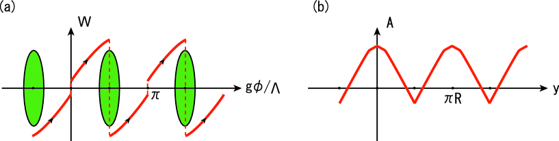
Figure 1: Non-BPS solution with unit winding number with the $S^{1}/(Z_{2}\times Z_{2})$ symmetry. Discontinuities in $W(\phi)$ at $g\phi/\Lambda=0,\pi$ ($\pi/2,3\pi/2$) correspond to positive (negative) boundary cosmological constants. (a) $\phi W$ plane, and (b)The function $A(y)$ in the warp factor.

If we place the first boundary at the vacuum point $\phi_{\rm R}=\Lambda\pi/(2g)$, we obtain a simplest model in the sense that the energy density at the second boundary at $\phi_{\rm R}=\Lambda\pi/(2g)$ is purely made of negative cosmological constant

$$\lambda=-4W(\phi_{\rm R}=\Lambda\pi/(2g)).$$ (2.47)

The magnitude of this negative cosmological constant becomes the same as the total energy of the wall centered at $\phi_{\rm R}=0$ in the limit of large separation of two boundaries. Since the solution admits $S^{1}/(Z_{2}\times Z_{2})$ symmetry, we call the coordinate at the second boundary $y=\pi R/2$. The behavior of this non-BPS solutions in the $W,\phi$ plane is illustrated in Fig.1(a). The corresponding function $A(y)$ in the warp factor is illustrated in Fig.1(b), where one should note that $A(y)$ is linear near the second boundary at $y=\pi R/2$, showing that only the boundary cosmological constant exists apart from the bulk cosmological constant there.

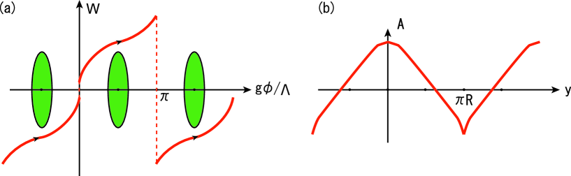
Figure 2: Non-BPS solution with unit winding number with the $S^{1}/Z_{2}$ symmetry. Discontinuities in $W(\phi)$ at $g\phi/\Lambda=0$ ($\pi$) correspond to positive (negative) boundary cosmological constants. (a) $\phi W$ plane, and (b)The function $A(y)$ in the warp factor.

As another solution, we can place the second boundary at $\phi_{\rm R}=\Lambda\pi/g$, where the active scalar field $\phi_{\rm R}$ develops another wall configuration. In this case, the negative cosmological constant $-4W(\phi_{\rm R}=\Lambda\pi/g)$ placed at the second boundary has magnitude which becomes twice the total energy of the wall centered at $\phi_{\rm R}=0$ in the limit of large separation of two boundaries. The behavior of this non-BPS solutions in the $W,\phi$ plane is illustrated in Fig.2(a). The corresponding function $A(y)$ in the warp factor is illustrated in Fig.2(b), where one should note that the function $A(y)$ has additional kink behavior deviating from the linear exponent near the second boundary at $y=\pi R$, showing that there is an additional smooth positive energy density centered around the boundary besides the negative boundary cosmological constant in contrast to the previous $S^{1}/(Z_{2}\times Z_{2})$ example in Fig.1.

3 Bosonic Fluctuation and the BPS Solution

A Bogomolo’nyi bound has been derived for the energy density of the BPS domain walls in $\mathcal{N}=1$ SUGRA in four-dimensional spacetime [20]. They used the generalized Israel-Nester-Witten tensor, which was originally applied to a simple proof of the positive ADM mass conjecture in general relativity. However, the ADM mass may not be well-defined for domain walls, since they are extended to infinity. Therefore it is presumably still useful to check that there is really stability of the fluctuation on our wall configuration even in the case of BPS solutions. We shall present a general formalism to analyze the modes and their stability, and then apply it to the fluctuations around the BPS background configurations in this section. The equations and procedures obtained in this section can also be used to the non-BPS background solutions with appropriate additional inputs, which is dealt with in Sec.4.

3.1 Mode equations for the bosonic sector

We start with the metric perturbation in the Newton gauge [30], [32] :

$$ds^{2}={\rm e}^{2A}\left(\eta_{\mu\nu}+h^{\rm TT}_{\mu\nu}+2B\eta_{\mu\nu}\right)dx^{\mu}dx^{\nu}+(1-2(D-3)B)dy^{2},$$ (3.1)

where $h^{\rm TT}_{\mu\nu}$ is transverse traceless $\eta^{\mu\nu}h^{\rm TT}_{\mu\nu}=0,\;\partial^{\mu}h^{\rm TT}_{\mu\nu}=0$. Some details for the procedure of this gauge fixing are given in Appendix A. This gauge is useful since the linearized equations become very simple. The linearized Einstein equations in $D$ space-time dimensions ($D=4$ in our specific model) read :

$$\left({\rm e}^{-2A}\square_{D-1}+\partial_{y}^{2}+(D-1)\dot{A}\partial_{y}\right)h^{\rm TT}_{\mu\nu}=0,$$ (3.2)

$$\left({\rm e}^{-2A}\square_{D-1}+\partial_{y}^{2}+(3D-5)\dot{A}\partial_{y}+2(D-3)\left((D-1)\dot{A}^{2}+\ddot{A}\right)\right)B=-{2\kappa^{2}\over D-2}\frac{dV_{\rm R}}{d\phi_{\rm R}}\varphi_{\rm R},$$ (3.3)

$$\left(\partial_{y}+(D-3)\dot{A}\right)B=-{2\kappa^{2}\over D-2}\kappa^{2}\dot{\phi}_{\rm R}\varphi_{\rm R},$$ (3.4)

where the first line comes from the traceless part of $(\mu,\nu)$ component of the linearized Einstein equations, the second line from the trace part of $(\mu,\nu)$ and the last from $(\mu,2)$ component. The $(2,2)$ component of the linearized equation is not shown, since it can be derived from Eqs.(3.2)-(3.4). The linearized field equations give :

$$\left({\rm e}^{-2A}\square_{D-1}+\partial_{y}^{2}+(D-1)\dot{A}\partial_{y}-\frac{1}{2}\frac{d^{2}V_{\rm R}}{d\phi_{\rm R}^{2}}\right)\varphi_{\rm R}=-2(D-2)\dot{\phi}_{\rm R}\partial_{y}B-(D-3)\frac{dV_{\rm R}}{d\phi_{\rm R}}B,$$ (3.5)

$$\left({\rm e}^{-2A}\square_{D-1}+\partial_{y}^{2}+(D-1)\dot{A}\partial_{y}-\frac{1}{2}\frac{\partial^{2}V}{\partial\phi_{\rm I}^{2}}\bigg{|}_{\rm background}\right)\varphi_{\rm I}=0,$$ (3.6)

where $\varphi_{\rm R(I)}$ denotes the real (imaginary) part of the fluctuation of the scalar field $\phi=\phi_{\rm R}+\varphi_{\rm R}+i\varphi_{\rm I}$ around the background field configuration $\phi_{\rm R}$. Notice that the solutions of the linearized Einstein equation automatically satisfy the linearized field equations for the active scalar field $\varphi_{\rm R}$. Therefore, the Eqs.(3.2)– (3.6) constitute the full set of independent linearized equations for the fields $h^{\rm TT}_{\mu\nu},\ B,\ \varphi_{\rm R}$ and $\varphi_{\rm I}$.

3.2 Tensor perturbation : localized massless graviton

First we show that the linearized equation for the transverse traceless mode (graviton) given in Eq.(3.2) can be brought into a Schrödinger form. It can again be rewritten into a form of the supersymmetric quantum mechanics (SQM) which ensures the stability of the system. For that purpose we change the coordinate $y$ into the conformally flat coordinate $z$ defined as

$$dz\equiv{\rm e}^{-A(y)}dy,\qquad ds^{2}={\rm e}^{2A(y)}\left(\eta_{\mu\nu}dx^{\mu}dx^{\nu}+dz^{2}\right).$$ (3.7)

We also redefine the field as $\tilde{h}^{\rm TT}_{\mu\nu}\equiv{\rm e}^{{D-2\over 2}A}h^{\rm TT}_{\mu\nu}$. In the following we use prime to denote a derivative in terms of $z$. Then the linearized equation (3.2) becomes

$$\square_{D-1}\tilde{h}^{\rm TT}_{\mu\nu}(x,z)=\left[-\partial_{z}^{2}+\mathcal{V}_{t}(z)\right]\tilde{h}^{\rm TT}_{\mu\nu}(x,z),\qquad\mathcal{V}_{t}(z)=\left({D-2\over 2}\right)^{2}A^{\prime}{{}^{2}}+{D-2\over 2}A^{\prime\prime},$$ (3.8)

where $\mathcal{V}_{t}(z)$ is the potential in this “Schrödinger” type equation. For our BPS background solution (2.36) the Schrödinger potential takes the form :

$$\mathcal{V}_{t}(y)=\big{[}\cosh\Lambda(y-y_{0})\big{]}^{-\frac{2k}{\Lambda}}\left[-\frac{k\Lambda}{\cosh^{2}\Lambda(y-y_{0})}+2k^{2}\tanh^{2}\Lambda(y-y_{0})\right],$$ (3.9)

where $4T^{3}\equiv 4g^{-2}\Lambda^{3}$ is the tension of the wall and $k=\kappa^{2}T^{3}$. Although our model contains three parameters $\Lambda,\ g$ and $\kappa$, this potential depends on only two parameters $k$ and $\Lambda$. If we take the thin wall limit where $\Lambda\rightarrow\infty$ fixing $4T^{3}$, we obtain (putting $y_{0}=0$)

$$\frac{\Lambda}{\cosh^{2}\Lambda y(z)}\rightarrow 2\delta(z),\quad\tanh^{2}\Lambda y(z)\rightarrow 1,\quad\left[\cosh\Lambda y(z)\right]^{-\frac{k}{\Lambda}}\rightarrow\frac{1}{\left(k|z|+1\right)^{2}},$$ (3.10)

with $kz={\rm sgn}(y){\rm e}^{k|y|}-1$. Thus the Schrödinger potential (3.9) becomes precisely the potential of the Randall-Sundrum model :

$$\mathcal{V}_{t}(z)\rightarrow\frac{2k^{2}}{\left(k|z|+1\right)^{2}}-2k\delta(z).$$ (3.11)

We find that the part of action quadratic in $\tilde{h}^{\rm TT}_{\mu\nu}$ has no $z$ dependent weight

$$S\sim\int dzd^{D-1}x\ \eta^{\mu\rho}\eta^{\nu\lambda}\tilde{h}^{\rm TT}_{\mu\nu}\left(\square_{D-1}+\partial_{z}^{2}-\frac{1}{2}\mathcal{V}_{t}\right)\tilde{h}^{\rm TT}_{\rho\lambda},$$ (3.12)

in conformity with the absence of the linear term [29] in $\partial_{z}$ in the Shrödinger type equation (3.8). We stress that this is written in terms of the conformal coordinate $z$ and the redefined field $\tilde{h}^{\rm TT}_{\mu\nu}$.

Defining mode equations by eigenvalue equations $\mathcal{H}_{t}\psi_{n}(z)=\left[-\partial_{z}^{2}+\mathcal{V}_{t}(z)\right]\psi_{n}(z)=m_{n}^{2}\psi_{n}(z)$ with mass squared eigenvalues $m_{n}^{2}$, and assuming mode functions $\psi_{n}(z)$ to form a complete set, the transverse traceless fields can be expanded into a set of effective fields $\hat{h}^{{\rm TT}(n)}_{\mu\nu}(x)$

$$\tilde{h}^{\rm TT}_{\mu\nu}(x,z)=\sum_{n}\hat{h}^{{\rm TT}(n)}_{\mu\nu}(x)\psi_{n}(z).$$ (3.13)

Then the above quadratic action (3.12) becomes

$$S\sim\sum_{n,k}\int dz\ \psi_{n}(z)\psi_{k}(z)\ \cdot\int d^{D-1}x\ \eta^{\mu\rho}\eta^{\nu\lambda}\hat{h}^{\rm TT(n)}_{\mu\nu}\left[\square_{D-1}-m_{k}^{2}\right]\hat{h}^{\rm TT(k)}_{\rho\lambda}.$$ (3.14)

Therefore the inner product for the mode function $\psi(z)$ should be defined as as

$$\langle\psi_{1}|\psi_{2}\rangle=\int dz\ \psi_{1}(z)\psi_{2}(z),$$ (3.15)

for which the usual intuition of quantum mechanics works.

The Hamiltonian $\mathcal{H}_{t}$ can now be expressed in a SQM form as follows

$$\mathcal{H}_{t}=Q_{t}^{\dagger}Q_{t},\qquad Q_{t}\equiv-\partial_{z}+{D-2\over 2}A^{\prime},\qquad Q_{t}^{\dagger}\equiv\partial_{z}+{D-2\over 2}A^{\prime},$$ (3.16)

where the “supercharge” $Q_{t}$ and $Q_{t}^{\dagger}$ are adjoint of each other at least for BPS background where no boundary condition has to be imposed. Therefore the Hamiltonian $\mathcal{H}_{t}$ is a nonnegative definite Hermitian operator, and its eigenvalues are nonnegative definite. Therefore we can conclude that the tensor perturbation has no tachyonic modes which destabilize the background field configurations at least for BPS solutions.

There are two possible zero modes in the tensor perturbation. One is the state which is annihilated by $Q_{t}|\tilde{h}^{\rm TT(+)}_{\mu\nu}\rangle=0$, and another is the state defined as $Q_{t}^{\dagger}\left(Q_{t}|\tilde{h}^{\rm TT(-)}_{\mu\nu}\rangle\right)=0$ where $Q_{t}|\tilde{h}^{\rm TT(-)}_{\mu\nu}\rangle\neq 0$. Then zero modes are of the form :

$$\tilde{h}^{\rm TT(0)}_{\mu\nu}(x,z)=\hat{h}^{\rm TT(+)}_{\mu\nu}(x)\ {\rm e}^{{D-2\over 2}A(z)}+\hat{h}^{\rm TT(-)}_{\mu\nu}(x)\ {\rm e}^{{D-2\over 2}A(z)}\int dz\ {\rm e}^{-(D-2)A(z)},$$ (3.17)

where $A(z)=A(y(z))$. Notice that we must verify the normalizability of the wave-function to obtain a physical massless effective field in the case of noncompact space such as our BPS background. In the case of non-BPS background, the boundary condition has to be verified, which we shall consider in Sec.4. The first mode $\hat{h}^{\rm TT(+)}_{\mu\nu}$ in Eq.(3.17) is normalizable if $\int dz\ {\rm e}^{(D-2)A(z)}<\infty$, corresponds to the graviton which is localized at the wall with a positive energy density. namely, if ${\rm e}^{(D-2)A}$ falls off faster than $|z|^{-1}$ [29]. For our BPS solution (2.36) the asymptotic behavior of the warp factor ${\rm e}^{A}$ is of order $|z|^{-1}$. Therefore we obtain a normalizable massless transverse traceless mode $\hat{h}^{\rm TT(+)}_{\mu\nu}$ which gives the physical graviton localized on the wall.

On the other hand, the second term $\hat{h}^{\rm TT(-)}_{\mu\nu}$ in Eq.(3.17) is not normalizable and is unphysical since $\left({\rm e}^{D-2\over 2}A\int dz\ {\rm e}^{-(D-2)A}\right)^{2}\sim|z|^{4}$ at $|z|\rightarrow\infty$ for our BPS solution. If there exists a regulator brane with a negative tension at some $y$, this mode can become normalizable and localizes at the negative tension brane in contrast to the graviton. If there are no bulk scalar fields (contrary to our model) as in the original Randall-Sundrum model of single wall, this zero mode corresponds to the physical massless field which was called radion in Ref.[27].

Our specific four-dimensional model of non-BPS wall gives a three-dimensional effective theory on the wall. Transverse traceless mode of graviton in three dimensions has no dynamical degree of freedom except possible topological modes. However, our formalism and analysis can be applied at each step to general $D$-dimensional theories, once we obtain the relevant non-BPS solutions in such theories. In that respect, we believe that our findings should still be useful.

Figure 3: The Schrödinger potential for the tensor perturbation in terms of the coordinate system $y$. We choose $y_{0}=0$ and $k=0.25$. The solid line has $\Lambda=3$ and the broken line has $\Lambda=1$.

The Schödinger potential can always be expressed in terms of $y$, but is difficult in terms of $z$ explicitly, since it is generally difficult to solve $dz={\rm e}^{-A}dy$ explicitly. If we express the potential in terms of $y$, we obtain a volcano type potential as shown in Fig.3. The width of the well is $\sim 2\Lambda^{-1}$ and the depth is $\sim k\Lambda$.

Next we turn to analysis of the massive Kaluza-Klein (KK) mode. There are no modes with negative mass squared in the tensor perturbation, as we have already shown. Since the Schrödinger potential (3.9) vanishes asymptotically ($z=\pm\infty$), all the massive KK modes are continuum scattering states with eigenvalues $m^{2}>0$. In order to examine the mode functions of the massive KK modes, we look into the region far from the wall, namely $\Lambda|y|\gg 1$. Since ${\rm e}^{A}\simeq{\rm e}^{-k|y|}$, $kz\simeq{\rm sgn}(y){\rm e}^{k|y|}-1$, we find that the Schrödinger potential becomes

$$\mathcal{V}_{t}(z)\simeq\frac{2k^{2}}{\left(k|z|+1\right)^{2}}\qquad\left(\Lambda|y|\gg 1\right).$$ (3.18)

This happens to be the same potential as that in the Randall-Sundrum single wall model [3], in spite of different spacetime dimensions. The wave functions of the continuum massive modes for this potential are known to be expressed as linear combinations of Bessel functions at the region far from the wall [3].

3.3 The active scalar perturbation

Next we study the perturbation of the active scalar field $\varphi_{\rm R}$. Notice that the fluctuation $\varphi_{\rm R}$ around the active scalar field background $\phi_{\rm R}$ can be reduced to the trace part $B$ of the metric perturbation through Eq.(3.4). Therefore we mainly concentrate on the trace (scalar) part of the metric perturbation $B$ in what follows. The linearized equation which contains only $B$ can be derived by combining Eq.(3.3) and (3.4) and using the background field equation :

$$\left[{\rm e}^{-2A}\square_{D-1}+\partial_{y}^{2}+\left((D-3)\dot{A}-2\frac{\ddot{\phi}_{\rm R}}{\dot{\phi}_{\rm R}}\right)\partial_{y}+2(D-3)\left(\ddot{A}-\dot{A}\frac{\ddot{\phi}_{\rm R}}{\dot{\phi}_{\rm R}}\right)\right]B=0.$$ (3.19)

In order to transform this into the Schrödinger form, we change the coordinate from $y$ to $z$ and redefine the field as $\tilde{B}\equiv{\rm e}^{{D-2\over 2}A}\phi_{\rm R}^{\prime}{{}^{-1}}B$. Substituting this into Eq.(3.19), we find the Schödinger type equation for the scalar perturbation;

$$\mathcal{H}_{e}\tilde{B}\equiv\left[-\partial_{z}^{2}+\mathcal{V}_{e}(z)\right]\tilde{B}=\square_{D-1}\tilde{B},$$ (3.20)

where the Schrödinger potential $\mathcal{V}_{e}(z)$ is defined by

$$\mathcal{V}_{e}(z)\equiv-\frac{\phi_{\rm R}^{\prime\prime\prime}}{\phi_{\rm R}^{\prime}}+2\left(\frac{\phi_{\rm R}^{\prime\prime}}{\phi_{\rm R}^{\prime}}\right)^{2}+(D-4){A^{\prime\prime}\phi_{R}^{\prime\prime}\over\phi_{R}^{\prime}}-{3D-10\over 2}A^{\prime\prime}+\left({D-2\over 2}\right)^{2}A^{\prime}{{}^{2}}.$$ (3.21)

Similarly to the tensor perturbation, the inner-product for the scalar perturbation $B$ should be defined in terms of the conformal coordinate $z$ and the redefined field $\tilde{B}$.

Plugging our solution (2.36) into this, we find

$$\mathcal{V}_{e}=\left[\cosh\Lambda(y-y_{0})\right]^{-\frac{2k}{\Lambda}}\left[\Lambda^{2}+k\Lambda\left(1+\frac{1}{\cosh^{2}\Lambda(y-y_{0})}\right)\right].$$ (3.22)

Figure 4: The Schrödinger potential for the scalar perturbation in terms of the coordinate system $y$. We choose $y_{0}=0$, and $k=0.25$. The solid line has $\Lambda=3$ and the broken line has $\Lambda=1$.

We stress that $\mathcal{V}_{e}$ can be expressed in terms of $y$, but not in terms of $z$, since it is generally difficult to solve $dz={\rm e}^{-A}dy$. This potential $\mathcal{V}_{e}$ has the following properties : i) it is positive definite, ii) it vanishes asymptotically at infinity, and iii) the height of $\mathcal{V}_{e}$ is of order $\Lambda^{2}$ as shown in Fig.4. From i) , it follows that there are no tachyonic modes since the wave function of such modes will necessarily diverge either at $y=\infty$ or $y=-\infty$. Therefore we can conclude that the background configuration (2.36) is stable under the active scalar perturbation. From ii), it follows that the spectrum of the massive modes is continuous starting from zero. From iii), the potential diverges at any finite point $y$ in the thin wall limit $(\Lambda\rightarrow\infty)$.

Though we can not find the exact solutions for the massive KK modes, zero modes can be found by rewriting the Hamiltonian (3.20) into SQM form as follows :

$$\mathcal{H}_{e}=Q_{e}^{\dagger}Q_{e},\quad\quad Q_{e}\equiv-\partial_{z}+\left[\log\left({\rm e}^{-{D-2\over 2}A}\dfrac{A^{\prime}}{\phi_{\rm R}^{\prime}}\right)\right]^{\prime},\quad Q_{e}^{\dagger}\equiv\partial_{z}+\left[\log\left({\rm e}^{-{D-2\over 2}A}\dfrac{A^{\prime}}{\phi_{\rm R}^{\prime}}\right)\right]^{\prime}.$$ (3.23)

To show this, we use the identity $\phi_{\rm R}^{\prime}\left(A^{\prime\prime\prime}-2A^{\prime}A^{\prime\prime}\right)=2\phi_{\rm R}^{\prime\prime}\left(A^{\prime\prime}-A^{\prime}{{}^{2}}\right)$. Similarly to the tensor perturbation there are two zero modes of $\mathcal{H}_{e}$ :

$$\tilde{B}^{(0)}(x,z)=\hat{B}^{(+)}(x)\ \frac{A^{\prime}}{\phi_{\rm R}^{\prime}}{\rm e}^{-{D-2\over 2}A}+\hat{B}^{(-)}(x)\ \frac{A^{\prime}}{\phi_{\rm R}^{\prime}}{\rm e}^{-{D-2\over 2}A}\int dz\ \frac{\phi_{\rm R}^{\prime}{{}^{2}}}{A^{\prime}{{}^{2}}}{\rm e}^{(D-2)A}.$$ (3.24)

Both zero modes are unphysical by the following reasons. The first term is unphysical, in the sense that this is eliminated by a gauge transformation preserving the Newton gauge (3.1) :

$$\xi_{2}=\hat{B}^{(+)}(x){{\rm e}^{-(D-3)A}\over D-3},\quad\xi_{\mu}=-\hat{B}^{(+)}_{,\mu}(x){{\rm e}^{2A}\over D-3}\int dy\ {\rm e}^{-(D-1)A},$$ (3.25)

where $\xi_{m}$ is an infinitesimal coordinate transformation parameters. The transformation law is given in Appendix A. The second term is unphysical since it diverges at infinity and is not normalizable as illustrated in Fig.7.

Next we turn to analysis for the massive KK modes. As we have mentioned above, massive modes are continuous from zero. Similarly to the tensor perturbation, properties of mode functions can be examined by analyzing the behavior of the potential in the region far from the wall. In the region where $|y|\Lambda\gg 1$, the Schrödinger potential (3.22) becomes :

$$\mathcal{V}_{e}(z)\simeq\frac{\Lambda^{2}+k\Lambda}{\left(k|z|+1\right)^{2}}.$$ (3.26)

This potential is very similar to the Schrödinger potential (3.18) for the tensor perturbation. Therefore all the massive modes are given by a linear combination of Bessel functions asymptotically at $|z|\rightarrow\infty$. Although these two Schrödinger potentials (3.18) and (3.26) have the same $z$ dependence asymptotically $|y|\Lambda\gg 1$, their behaviors in the thin wall limit are very different. The potential (3.18) depends only on $k$ (fixed in the thin-wall limit), but not on $\Lambda$. On the other hand, the potential (3.26) is proportional to polynomials in $\Lambda$. Therefore, the latter diverges in thin wall limit whereas the former is finite. This can be understood as follows. The perturbation of the trace part of the metric $B$ is related to the active scalar field perturbation $\varphi_{\rm R}$ through Eq.(3.4). Since all the massive KK modes associated with the active scalar field become infinitely heavy in the thin wall limit, the massive KK modes for the perturbation of the trace part of the metric freeze simultaneously. In this limit only the tensor perturbations remain which correspond to the known modes of the RS model .

The zero modes $\hat{B}^{(+)}(x)\dfrac{A^{\prime}}{\phi_{\rm R}^{\prime}}{\rm e}^{-{D-2\over 2}A}$ of the fluctuation of the trace part of the metric $B$ in Eq.(3.24) can be translated into the perturbation of the active scalar field $\varphi_{\rm R}$ by means of Eq.(3.4) :

$$\varphi_{\rm R}^{(0)}(x,y)=\hat{\varphi}_{\rm R}^{(+)}(x)\ \dot{\phi}_{\rm R}{\rm e}^{-(D-3)A}\rightarrow\hat{\varphi}_{\rm R}^{(+)}(x)\ \dot{\phi}_{\rm R},\quad\left(\kappa\rightarrow 0\right).$$ (3.27)

where $\hat{\varphi}_{\rm R}^{(+)}(x)\equiv(D-2)\hat{B}_{\rm R}^{(+)}(x)/2$. In weak gravity limit $(\kappa\rightarrow 0)$, ${\rm e}^{A}$ reduces to a constant. Then we find that this zero mode is localized on the wall and that it corresponds to the Nambu-Goldstone boson corresponding to the spontaneously broken translational invariance.

3.4 Analysis for the perturbation about $\phi_{\rm I}$

In our tree level solution the imaginary part of the scalar field $\phi$ vanishes identically and does not contribute to the energy momentum tensor. Therefore it does not affect the spacetime geometry. We shall call scalar fields with no nontrivial field configuration as inert field. In the linear order of perturbations we found that the fluctuation $\varphi_{\rm I}$ of this inert field decouples from any other fluctuations, as shown in Eq.(3.6).

In order to find the spectrum of $\varphi_{\rm I}$, we first bring Eq.(3.6) into a Schrödinger form by changing the coordinate from $y$ to $z$ and redefining the field $\tilde{\varphi}_{\rm I}\equiv{\rm e}^{{D-2\over 2}A}\varphi_{\rm I}$. Then we obtain

$$\mathcal{H}_{\rm I}\tilde{\varphi}_{I}\equiv\left[-\partial_{z}^{2}+\mathcal{V}_{\rm I}(z)\right]\tilde{\varphi}_{\rm I}=\square_{D-1}\tilde{\varphi}_{\rm I},\quad\mathcal{V_{\rm I}}(z)\equiv\mathcal{V}_{t}(z)+{\rm e}^{2A}\dfrac{1}{2}\dfrac{\partial^{2}V}{\partial\phi_{\rm I}^{2}}\bigg{|}.$$ (3.28)

where ${\cal V}_{t}(z)$ is the potential for transverse traceless part of the metric defined in Eq.(3.8). To obtain more concrete informations on the spectrum, we need to examine properties of each model. For our model we find

$$\frac{1}{2}\frac{\partial^{2}V}{\partial\phi_{\rm I}^{2}}\bigg{|} = \Lambda^{2}+\frac{\kappa^{2}\Lambda^{4}}{g^{2}}\left(1+2\cos^{2}\frac{g}{\Lambda}\phi_{\rm R}\right)-\frac{2\kappa^{4}\Lambda^{6}}{g^{4}}\sin^{2}\frac{g}{\Lambda}\phi_{\rm R}$$ (3.29)

We shall discuss generic property of this inert scalar for the non-BPS background in Sec.4.

If we choose the BPS solution as our background, we can rewrite the potential by using the BPS equations (2.35)

$$\frac{1}{2}\frac{\partial^{2}V}{\partial\phi_{\rm I}^{2}}\bigg{|} = \Lambda^{2}+2k\Lambda-2\ddot{A}-2\dot{A}^{2},$$ (3.30)

Then the Schrödinger potential $\mathcal{V}_{\rm I}$ takes the form :

$$\mathcal{V}_{\rm I}=A^{\prime}{{}^{2}}-A^{\prime\prime}+{\rm e}^{2A}\left(\Lambda^{2}+2k\Lambda\right).$$ (3.31)

We illustrate $\mathcal{V}_{I}$ in terms of $y$ in Fig.5. For vanishing gravitational coupling $\kappa\rightarrow 0$, $\mathcal{V}_{\rm I}$ reduces to a constant $\Lambda^{2}$, which agrees with the model of global SUSY in Ref.[24]. On the other hand, the potential $\mathcal{V}_{\rm I}$ acquires regions of negative values when $\kappa$ becomes large.

Figure 5: The Schrödinger potential for the perturbation of the imaginary part of the scalar field in terms of the coordinate system $y$. We choose $y_{0}=0$ and $\Lambda=1$. The bold line has $k=1$, the solid line has $k=0.25$ and the broken line has $k=0.05$.

In the case of the BPS background, we can show that there are no tachyonic modes in this inert scalar sector with the aid of the SQM. Let us introduce a supercharge as $Q_{\rm I}=-\partial_{z}-A^{\prime}$ and $Q_{\rm I}^{\dagger}=\partial_{z}-A^{\prime}$. Then the Hamiltonian $\mathcal{H}_{\rm I}$ can be rewritten as

$$\mathcal{H}_{\rm I}=Q_{\rm I}^{\dagger}Q_{\rm I}+{\rm e}^{2A}\left(\Lambda^{2}+2k\Lambda\right).$$ (3.32)

The first term is a nonnegative definite Hermitian operator and the second term is never negative. Therefore, we can conclude that eigenvalues of $\mathcal{H}_{\rm I}$ are always nonnegative and there are no tachyonic mode.

4 Stability of Non-BPS multi-Walls

For non-BPS solutions, the positivity of the energy of the fluctuation and the associated stability is entirely nontrivial. In the limit of vanishing gravitational coupling, however, our supergravity model reduces to a global SUSY model that has been shown to be stable [24]. Since the mass gap in the global SUSY model should not disappear even if we switch on the gravitational coupling infinitesimally, the massive scalar fluctuations in the global SUSY model should remain massive at least for small gravitational coupling. On the other hand, we need to watch out a possible new tachyonic instability associated with the metric fluctuations.

As for the transverse traceless part of the metric, we have already shown that there are two possible zero mode candidates $\hat{h}^{\rm TT(+)}_{\mu\nu}(x)\ {\rm e}^{A(z)}$ and $\hat{h}^{\rm TT(-)}_{\mu\nu}(x)\ {\rm e}^{A(z)}\int dz\ {\rm e}^{-2A(z)}$ in Eq.(3.17). In the non-BPS solution, we no longer need to worry about the normalizability of the wave function. Instead, we need to satisfy the boundary condition imposed by the presence of the boundary cosmological constants. To impose the boundary condition, we have to use coordinate system which is more more appropriate to specify the position of the boundary. This is achieved by going to the Gaussian normal coordinates [30]. We have been using the Newton gauge to study the mass spectrum in the Shrödinger type equation. We can follow the argument in Ref.[30] to obtain general coordinate transformations $\xi_{m}$ from the Newton gauge to the Gaussian normal gauge :

$$\xi_{2}(x,y)={1\over 2}\int_{0}^{y}dy^{\prime}h_{22}+\bar{\xi}_{2}^{(\pm)}(x),$$ (4.1)

$$\xi_{\mu}(x,y)=-{1\over 2}\int_{y^{(\pm)}}^{y}dy^{\prime}e^{-2A}\int_{y^{(\pm)}}^{y^{\prime}}dy^{\prime\prime}h_{22,\mu}-\bar{\xi}_{2,\mu}^{(\pm)}\int_{y^{(\pm)}}^{y}dy^{\prime}e^{-2A}+\bar{\xi}_{\mu}^{(\pm)}(x),$$ (4.2)

where $\bar{\xi}_{2}^{(\pm)},\bar{\xi}_{\mu}^{(\pm)}$ depend on $x$ only. Boundary conditions in the Newton gauge are found to be [30]

$$\left[\partial_{y}h_{\mu\nu}^{TT}+2e^{-2A}\bar{\xi}_{2,\mu,\nu}^{(\pm)}\right]_{y^{(\pm)}-0}^{y^{(\pm)}+0}=0,$$ (4.3)

$$\left[\left(\partial_{y}+\dot{A}\right)h_{22}+2\ddot{A}\bar{\xi}_{2}^{(\pm)}\right]_{y^{(\pm)}-0}^{y^{(\pm)}+0}=0.$$ (4.4)

We find that the former mode $\hat{h}^{\rm TT(+)}_{\mu\nu}(x)\ {\rm e}^{A(z)}$ receives no constraint from the boundary condition, and is still a physical massless mode localized on the wall which should be regarded as the graviton in the effective theory. The latter mode $\hat{h}^{\rm TT(-)}_{\mu\nu}(x)\ {\rm e}^{A(z)}\int dz\ {\rm e}^{-2A(z)}$ is constrained by the boundary condition (4.3). Since the constraint (4.3) and (4.4) relate $\bar{\xi}_{2}^{(\pm)}$ to $\hat{h}^{(-)}_{\mu\nu}$ and $\hat{h}_{22}(x)$, this mode should be classified as a scalar type perturbation. On the other hand, $\hat{h}^{(-)}_{\mu\nu}$ can be gauged away through the gauge transformation (3.25), which preserves the Newton gauge. Therefore this mode becomes unphysical in the presence of the bulk scalar field like in our model. Since $\bar{\xi}_{2}$ corresponds to the physical distance between the two branes [27], our system automatically incorporates the stabilization mechanism without an additional bulk scalar fields. In the thin wall limit, the wall scalar field freezes out and the fluctuation of the scalar field ceases to be related to the scalar perturbation of the metric, so that $\hat{h}_{\mu\nu}^{(-)}$ can no longer be gauged away. As a result of restoration of $\hat{h}_{\mu\nu}^{(-)}$, any distance between two walls is admitted as classical solutions and the model becomes meta-stable.

To evaluate the mass spectrum of massive modes, we use the small width approximation. Then the asymptotic behavior of the potential gives the wave functions expressed by means of the Bessel functions as in the Randall-Sundrum model. These eigenvalue spectrum is approximately equally spaced just like the plane wave solutions. These (almost) continuum modes should give the corrections to the effects of localized graviton, similarly to the Randall-Sundrum model. Therefore we obtain a massless graviton localized on the wall and a tower of massive KK modes for transverse traceless part of the metric.

Since the active scalar field $\varphi_{\rm R}$ exhibits a mass gap without any tachyon, we expect that there should be no tachyonic instability at least for small enough gravitational coupling. We have found in Eq.(3.4) that the active scalar field $\varphi_{\rm R}$ can be reduced to the trace part of the metric $B$. This implies that there should be no tachyon in the transverse traceless mode as well at least for small gravitational coupling, since both degrees of freedom represent one and the same dynamical degree of freedom. In fact, we have observed that the potential ${\cal V}_{e}$ defined in Eq.(3.21) is everywhere positive and has no tachyon.

There are two possible zero mode candidates as given in Eq.(3.24). However, both of them are unphysical by the following reason. The first one can be eliminated by a gauge transformation. The second one has now no problem of normalization, since the extra dimension is now a finite interval, but it cannot satisfy the boundary conditions [30].

To evaluate the mass of the lightest scalar particle, which is usually called radion, we use the thin-wall approximation where the wall width is assumed to be small compared to the radius of compactification $R$. To make this approximation, we separate the potential (3.21) for the trace part of the metric fluctuation into unperturbed and perturbation as

$$\mathcal{V}_{e}(z)\equiv\mathcal{V}_{e}^{(0)}(z)+\mathcal{V}_{e}^{(1)}(z),$$ (4.5)

$$\mathcal{V}_{e}^{(0)}(z)=\phi_{\rm R}^{\prime}e^{{D-4\over 2}A}\left({e^{-{D-4\over 2}A}\over\phi_{\rm R}^{\prime}}\right)^{\prime\prime},\qquad\mathcal{V}_{e}^{(1)}(z)={D-3\over D-2}2\kappa^{2}\left(\phi_{\rm R}^{\prime}\right)^{2},$$ (4.6)

where we considered in $D$-dimensions instead of $4$ dimensions. The zero-th order eigenfunction for the lowest eigenvalue is found to be

$$\tilde{B}^{(0)}(z)={{\cal N}\over{\rm e}^{{D-2\over 2}A}\phi_{\rm R}^{\prime}},$$ (4.7)

with the vanishing eigenvalue $(m_{0}^{(0)})^{2}=0$ and a normalization factor ${\cal N}$. The first order eigenfunction is given by

$$\tilde{B}^{(1)}(z)={{\cal N}\over{\rm e}^{{D-4\over 2}A}\phi_{\rm R}^{{}^{\prime}}}\int^{z}dz^{\prime}{\rm e}^{(D-4)A}\phi_{\rm R}^{{}^{\prime}2}\int^{z^{\prime}}dz^{\prime\prime}{\rm e}^{-(D-4)A}\phi_{\rm R}^{{}^{\prime}-2}\left(\mathcal{V}_{e}^{(1)}(z)-(m_{0}^{(1)})^{2}\right),$$ (4.8)

where the first correction to the mass squared eigenvalue is denoted as $(m_{0}^{(1)})^{2}$. By using Eq.(3.4), the trace part of the metric can be transformed into the active scalar fluctuation $\varphi_{\rm R}$ as

$$\varphi_{0}^{(1)}(y)=-{D-2\over\kappa^{2}}{\cal N}\dot{\phi}_{0}\int_{0}^{y_{(+)}}dy^{\prime}\left({D-3\over D-2}\kappa^{2}{\rm e}^{-(D-3)A}-{(m_{0}^{(1)})^{2}{\rm e}^{-(D-1)A}\over 2\dot{\phi}_{\rm R}^{2}}\right),$$ (4.9)

where the position of the wall is at $y=0$ and the boundary with the negative cosmological constant is $y_{(+)}$. To satisfy the correct boundary conditions, we have to require that this first order eigenfunction $\varphi_{0}^{(1)}$ should vanish at the boundary [30]. This determines the first order mass squared as

$$(m_{0}^{(1)})^{2}=2\kappa^{2}\frac{D-3}{D-2}\frac{\displaystyle\int_{0}^{y_{(+)}}dy\ {\rm e}^{-A}}{\displaystyle\int_{0}^{y_{(+)}}dy\ \dfrac{{\rm e}^{-3A}}{\dot{\phi}_{0}^{2}}},$$ (4.10)

Taking $D=4$ as in our model, and applying to the case of the first example of non-BPS background in Eq.(2.47) with the symmetry $Z_{2}\times Z_{2}$, we should identify $y_{(+)}=\pi R/2$ and obtain

$$m^{2}_{0}\approx 8\Lambda^{2}e^{-(1+\alpha^{2})\pi\Lambda R}\left(1+{3\over 2}\alpha^{2}\right)2^{\alpha^{2}},\qquad\alpha^{2}\equiv{\kappa^{2}T^{3}\over\Lambda},$$ (4.11)

where $4T^{3}$ is the tension (energy density) of the wall. For the other background solution with the $Z_{2}\times Z_{2}$ symmetry, we should identify the boundary with the negative cosmological constant as $y_{(+)}=\pi R$, and obtain the same result. It is interesting to note that the mass scale is given by the inverse wall width $\Lambda$, and that it becomes exponentially light as a function of the distance between the walls, even though the radion mass receives a complicated gravitational corrections. It is appropriate to fix the wall tension and the gravitational coupling in taking the small width limit $\Lambda R\rightarrow\infty$. Then we obtain a simple mass formula in the limit

$$m^{2}_{0}\approx 8\Lambda^{2}e^{-\pi\Lambda R}\rightarrow 0.$$ (4.12)

This characteristic feature of lightest massive scalar fluctuation is precisely the same as the global SUSY case [15]. The lightest massive mode in that case results from the fact that two walls have no communication when they are far apart, and the translation zero modes of each wall becomes massless as the separation between walls goes to infinity.

The mass spectrum of the inert scalar fluctuations $\varphi_{\rm I}$ is determined by the Schrördinger form of the eigenvalue problem (3.28) with the potential $\mathcal{V_{\rm I}}(z)$. The potential has the same term as the transverse traceless mode $\mathcal{V_{\rm t}}(z)$ with an additional term $\frac{1}{2}\frac{\partial^{2}V}{\partial\phi_{\rm I}^{2}}\bigg{|}$ in Eq.(3.29) which is nonnegative definite provided the gravitational coupling is not too strong $\kappa\leq{g\over\Lambda}$

$$\frac{1}{2}\frac{\partial^{2}V}{\partial\phi_{\rm I}^{2}}\bigg{|} = \Lambda^{2}\left(1+3\frac{\kappa^{2}\Lambda^{2}}{g^{2}}\right)-2\frac{\kappa^{4}\Lambda^{4}}{g^{2}}\left(1+\frac{\kappa^{2}\Lambda^{2}}{g^{2}}\right)\sin^{2}\frac{g}{\Lambda}\phi_{\rm R}$$ (4.13)

$$\geq \Lambda^{2}\left(1-\frac{\kappa^{2}\Lambda^{2}}{g^{2}}\right)\left(1+2\frac{\kappa^{2}\Lambda^{2}}{g^{2}}\right)\geq 0.$$

Therefore inert scalar does not produce any additional tachyonic instability.

5 Fermions

In the previous two sections, we focused on the stability of BPS and Non-BPS wall configurations and studied its fluctuations. In this section, we turn to the fermionic part of the model and study its fluctuation. We shall consider only the BPS solutions for simplicity, since it allows massless gravitino, whereas the non-BPS solutions do not. The part of the Lagrangian (2.1) quadratic in fermion fields (with arbitrary powers of bosons) can be rewritten as

$$e^{-1}{\cal L}_{{\rm fermion}}^{{\rm quadratic}} = -i{\rm e}^{-A}\bar{\chi}\bar{\sigma}^{\underline{\mu}}{\cal D}_{\mu}\chi-i\bar{\chi}\bar{\sigma}^{\underline{2}}{\cal D}_{2}\chi+\varepsilon^{\underline{\kappa 2\mu\nu}}{\rm e}^{-3A}\bar{\psi}_{\kappa}\bar{\sigma}_{\underline{2}}\tilde{{\cal D}}_{\mu}\psi_{\nu}+\varepsilon^{\underline{\kappa\lambda 2\nu}}{\rm e}^{-2A}\bar{\psi}_{\kappa}\bar{\sigma}_{\underline{\lambda}}\tilde{{\cal D}}_{2}\psi_{\nu}$$ (5.1)

$$+\varepsilon^{\underline{2\lambda\mu\nu}}{\rm e}^{-2A}\bar{\psi}_{2}\bar{\sigma}_{\underline{\lambda}}\tilde{{\cal D}}_{\mu}\psi_{\nu}+\varepsilon^{\underline{\kappa\lambda\mu 2}}{\rm e}^{-2A}\bar{\psi}_{\kappa}\bar{\sigma}_{\underline{\lambda}}\tilde{{\cal D}}_{\mu}\psi_{2}$$

$$-\frac{\kappa}{\sqrt{2}}{\rm e}^{-A}\dot{\phi}^{*}\chi\sigma^{\underline{\mu}}\bar{\sigma}^{\underline{2}}\psi_{\mu}-\frac{\kappa}{\sqrt{2}}{\rm e}^{-A}\dot{\phi}\bar{\chi}\bar{\sigma}^{\underline{\mu}}\sigma^{\underline{2}}\bar{\psi}_{\mu}+\frac{\kappa}{\sqrt{2}}\dot{\phi}^{*}\chi\psi_{2}+\frac{\kappa}{\sqrt{2}}\dot{\phi}\bar{\chi}\bar{\psi}_{2}$$

$$-\kappa^{2}{\rm e}^{{\kappa^{2}\over 2}\phi^{*}\phi}\biggl{[}P^{*}{\rm e}^{-2A}\psi_{\mu}\sigma^{\underline{\mu\nu}}\psi_{\nu}+P{\rm e}^{-2A}\bar{\psi}_{\mu}\bar{\sigma}^{\underline{\mu\nu}}\bar{\psi}_{\nu}+2{\rm e}^{-A}(P^{*}\psi_{\mu}\sigma^{\underline{\mu 2}}\psi_{2}+P\bar{\psi}_{\mu}\sigma^{\underline{\mu 2}}\bar{\psi}_{2})$$

$$+{\rm e}^{-A}\frac{i\kappa}{\sqrt{2}}(D_{\phi}P\chi\sigma^{\underline{\mu}}\bar{\psi}_{\mu}+D_{\phi^{*}}P^{*}\bar{\chi}\bar{\sigma}^{\underline{\mu}}\psi_{\mu})+\frac{i\kappa}{\sqrt{2}}(D_{\phi}P\chi\sigma^{\underline{2}}\bar{\psi}_{2}+D_{\phi^{*}}P^{*}\bar{\chi}\bar{\sigma}^{\underline{2}}\psi_{2})$$

$$+\frac{1}{2}({\cal D}_{\phi}D_{\phi}P\chi^{2}+{\cal D}_{\phi^{*}}D_{\phi^{*}}P^{*}\bar{\chi}^{2})\biggr{]}.$$

The terms in the fourth line is quadratic in gravitino without any derivatives, which can be regarded as mass terms for gravitino. We find that they are $Z_{2}$ odd under $\phi\rightarrow-\phi$. In this respect, our model provides an explicit realization of the condition to have a smooth limit of vanishing width of the wall [21] and in agreement with one version of the five-dimensional supergravity on the orbifold [19]. For our modified superpotential $P$ given in Eq.(2.29), $D_{\phi}P$ and ${\cal D}_{\phi}D_{\phi}P$ are of the form:

$$D_{\phi}P = {\rm e}^{-\frac{\kappa^{2}}{2}\phi^{2}}\left[\kappa^{2}(\phi^{*}-\phi)\frac{\Lambda^{3}}{g^{2}}{\rm sin}\frac{g}{\Lambda}\phi+\frac{\Lambda^{2}}{g}{\rm cos}\frac{g}{\Lambda}\phi\right],$$ (5.2)

$${\cal D}_{\phi}D_{\phi}P = 2\kappa^{2}(\phi^{*}-\phi)\partial_{\phi}P-\left(\kappa^{2}+\kappa^{4}(\phi^{2}-\phi^{*2})+\frac{g^{2}}{\Lambda^{2}}\right)P,$$ (5.3)

$$= {\rm e}^{-\frac{\kappa^{2}}{2}\phi^{2}}\left[-\left(\kappa^{2}+\frac{g^{2}}{\Lambda^{2}}-\kappa^{4}(\phi-\phi^{*})^{2}\right)\frac{\Lambda^{3}}{g^{2}}{\rm sin}\frac{g}{\Lambda}\phi+2\kappa^{2}(\phi^{*}-\phi)\frac{\Lambda^{2}}{g}{\rm cos}\frac{g}{\Lambda}\phi\right].$$ (5.4)

5.1 Gravitino

In this subsection, we will explore a massless gravitino which is a superpartner of the massless localized graviton under the SUGRA transformation with the conserved Killing spinor (2.39). Before studying equations of motion for gravitino, we will supertransform the wave function of the localized massless graviton to find conditions that the physical gravitino should satisfy. Let us focus on SUGRA transformation law for vierbein in Eq.(2.12),

$$\delta_{\zeta}e_{m}{{}^{\underline{a}}}=i\kappa\left(\zeta\sigma^{\underline{a}}\bar{\psi}_{m}+\bar{\zeta}\bar{\sigma}^{\underline{a}}\psi_{m}\right).$$ (5.5)

The preserved SUSY along the Killing spinor $\zeta{(K)}$ in Eq.(2.39) with $\theta=\pi/2$ is given by

$$\zeta^{\alpha}{(K)} = -i\bar{\zeta}_{\dot{\alpha}}(K)\bar{\sigma}^{2\dot{\alpha}\alpha}=i{\rm e}^{A/2}[\epsilon_{2},-\epsilon_{1}],$$ (5.6)

$$\bar{\zeta}_{\dot{\alpha}}(K) = -i\zeta^{\alpha}{(K)}\sigma^{2}_{\alpha\dot{\alpha}}=i{\rm e}^{A/2}[-\epsilon_{1},-\epsilon_{2}].$$ (5.7)

Denoting the fluctuations $h_{mn}$ of the metric around the background spacetime metric $g_{mn}^{\rm background}\equiv diag({\rm e}^{2A}\eta_{\mu\nu},1)$ as $g_{mn}=g_{mn}^{\rm background}+h_{mn}$, the following linearized 3D SUGRA transformations with the Killing spinor $\zeta(K)$ are obtained for the metric fluctuations $\delta h_{mn}=\delta(e_{m}{}^{\underline{a}}e_{n\underline{a}})=\delta e_{m}{}^{\underline{a}}e_{n\underline{a}}+e_{m\underline{a}}\delta e_{n}{}^{\underline{a}}$

$$\delta_{\zeta(K)}h_{\mu\nu} = i\kappa{\rm e}^{A}\zeta(K)(\sigma_{\underline{\mu}}\bar{\psi}_{\nu}-i\sigma^{\underline{2}}\bar{\sigma}_{\underline{\mu}}\psi_{\nu}+\sigma_{\underline{\nu}}\bar{\psi}_{\mu}-i\sigma^{\underline{2}}\bar{\sigma}_{\underline{\nu}}\psi_{\mu}),$$ (5.8)

$$\delta_{\zeta(K)}h_{2\mu} = i\kappa\zeta(K)\left\{\sigma_{\underline{2}}\bar{\psi}_{\mu}+i\psi_{\mu}+(\sigma_{\underline{\mu}}\bar{\psi}_{2}-i\sigma^{\underline{2}}\bar{\sigma}_{\underline{\mu}}\psi_{2}){\rm e}^{A}\right\},$$ (5.9)

$$\delta_{\zeta(K)}h_{22} = 2i\kappa\zeta(K)(\sigma_{2}\bar{\psi}_{2}+i\psi_{2}).$$ (5.10)

In sect.3.2, we have imposed the gauge fixing condition (Newton Gauge) for graviton

$$h_{22}=-\frac{1}{3}{\rm e}^{-2A}\eta^{\mu\nu}h_{\mu\nu}\equiv-\frac{1}{3}h,$$ (5.11)

$$h_{2\mu}=0.$$ (5.12)

We can algebraically decompose $h_{\mu\nu}$ into traceless part ${\rm e}^{2A}h_{\mu\nu}^{TT}$ and trace part $h$. We have found that the localized graviton zero mode is contained in the traceless part

$$\eta^{\mu\nu}h_{\mu\nu}=0.$$ (5.13)

Equation of motion shows that the localized graviton zero mode also satisfies the transverse condition:

$$\eta^{\lambda\mu}\partial_{\lambda}h_{\mu\nu}=0.$$ (5.14)

The matter fermion of course do not have the graviton zero mode : $\varphi=0$.

It is useful to decompose Weyl spinors in four dimensions into two 2-component Majorana spinors in three dimensions. For instance gravitinos $\psi_{m}$ are decomposed into two 2-component Majorana spinor-vectors $\psi_{m}^{(1)}$ and $\psi_{m}^{(2)}$ (real and imaginary part of the Weyl spinor-vector)

$$\psi_{m\alpha}^{(1)}\equiv\psi_{m\alpha}-i\sigma^{2}_{\alpha\dot{\alpha}}\bar{\psi}_{m}^{\dot{\alpha}}=-i\sigma^{2}_{\alpha\dot{\alpha}}\bar{\psi}_{m}^{(1)\dot{\alpha}},$$ (5.15)

$$\psi^{(2)}_{m\alpha}\equiv\psi_{m\alpha}+i\sigma^{2}_{\alpha\dot{\alpha}}\bar{\psi}_{m}^{\dot{\alpha}}=i\sigma^{2}_{\alpha\dot{\alpha}}\bar{\psi}_{m}^{(2)\dot{\alpha}}.$$ (5.16)

Similarly to the traceless and trace part decomposition of graviton (symmetric tensor), gravitino (vector-spinor) can also be algebraically decomposed into its traceless part $\psi_{\mu}^{T}$ and trace part $\bar{\psi}$ as

$$\psi_{\mu}=\psi_{\mu}^{T}-{1\over 3}\sigma_{\underline{\mu}}\bar{\psi},\qquad\bar{\sigma}^{\underline{\mu}}\psi_{\mu}^{T}=0,\qquad\bar{\sigma}^{\underline{\mu}}\psi_{\mu}=\bar{\psi}.$$ (5.17)

Let us make a SUGRA transformations of the physical state conditions (5.11)–(5.14) for gravitons with the conserved Killing spinor $\zeta(K)$ in Eq.(5.7). The SUGRA transformations with $\zeta(K)$ of Eqs.(5.11), (5.12) (5.13) give

$$0=\delta_{\zeta(K)}\left(h_{22}+\frac{1}{3}h\right)=2i\kappa\zeta(K)\left(\sigma_{\underline{2}}\bar{\psi}_{2}^{(1)}+\frac{1}{3}{\rm e}^{-A}\sigma^{\underline{\mu}}\bar{\psi}_{\mu}^{(2)}\right),$$ (5.18)

$$0 = \delta_{\zeta(K)}h_{2\mu}=i\kappa\zeta\left(\sigma_{\underline{2}}\bar{\psi}_{\mu}^{(1)}+{\rm e}^{A}\sigma_{\underline{\mu}}\bar{\psi}_{2}^{(2)}\right).$$ (5.19)

$$0 = \delta_{\zeta(K)}\eta^{\mu\nu}h_{\mu\nu}=2i\kappa{\rm e}^{-A}\zeta\sigma^{\underline{\mu}}\bar{\psi}_{\mu}^{(2)}.$$ (5.20)

These result suggest the most natural gauge fixing condition for local gauge SUGRA transformations

$$\psi_{2}=0,$$ (5.21)

which can always be chosen. Then, the above gauge fixing conditions (5.18)–(5.20) are translated as $\bar{\psi}_{\mu}^{(1)}=0$ and the traceless condition for $\psi^{(2)}$

$$\sigma^{\underline{\mu}}\bar{\psi}_{\mu}=0.$$ (5.22)

Therefore we expect that the localized massless gravitino should be contained in the traceless part of $\psi_{\mu}^{(2)}$. The SUGRA transformation of the remaining condition (5.14) gives the transverse condition for the $\psi_{\mu}^{(2)}$. Similarly to the graviton case, the localized gravitino should not have matter component

$$\chi=0.$$ (5.23)

Let us now examine the equations of motion for gravitino $\psi_{\mu}$ coupled with the matter fermion $\chi$, which are obtained by varying the action (5.1). If we impose the conditions (5.21), (5.22), and (5.23) on the gravitino equations of motion, we obtain

$$0 = {\rm e}^{-3A}\varepsilon^{\underline{\mu 2\rho\nu}}\bar{\sigma}_{\underline{2}}\partial_{\rho}\psi_{\nu}+{\rm e}^{-2A}\left(-\frac{1}{2}\dot{A}\varepsilon^{\underline{\mu 2\rho\nu}}\bar{\sigma}_{\underline{\rho}}\psi_{\nu}+\varepsilon^{\underline{\mu\rho 2\nu}}\bar{\sigma}_{\underline{\rho}}\partial_{2}\psi_{\nu}-\kappa^{2}{\rm e}^{{\kappa^{2}\over 2}\phi^{*}\phi}P\bar{\sigma}^{\mu\nu}\bar{\psi}_{\nu}\right)$$ (5.24)

$$= {\rm e}^{-3A}\varepsilon^{\underline{\mu 2\rho\nu}}\bar{\sigma}_{\underline{2}}\partial_{\rho}\psi_{\nu}+{\rm e}^{-2A}\left[-\varepsilon^{\underline{\mu 2\rho\nu}}\bar{\sigma}_{\underline{\rho}}\left(\partial_{2}+\frac{1}{2}\dot{A}\right)\psi_{\nu}+\dot{A}\eta^{\mu\nu}\bar{\psi}_{\nu}\right],$$

where we have used the BPS equation (2.25) for background fields. Possible zero mode should give a vanishing eigenvalue for the operator in the parenthesis :

$$0 = -\varepsilon^{\underline{\mu 2\rho\nu}}\bar{\sigma}_{\underline{\rho}}\left(\partial_{2}+\frac{1}{2}\dot{A}\right)\psi_{\nu}+\dot{A}\eta^{\mu\nu}\bar{\psi}_{\nu}=-i\eta^{\mu\nu}\bar{\sigma}^{\underline{2}}\left(\partial_{2}+{\dot{A}\over 2}\right)\psi_{\nu}+\dot{A}\eta^{\mu\nu}\bar{\psi}_{\nu}$$ (5.25)

where $\varepsilon^{\underline{\mu\rho 2\nu}}\bar{\sigma}_{\underline{\rho}}=i(\bar{\sigma}^{\underline{\mu}}\sigma^{\underline{2}}\bar{\sigma}^{\underline{\nu}}-\eta^{\underline{\mu\nu}}\bar{\sigma}^{\underline{2}})$ is used in the second equality. In terms of the 2-component Majorana spinors (5.15) and (5.16), we obtain

$$\left(\partial_{2}+\frac{3}{2}\dot{A}\right)\bar{\psi}^{(1)TT}_{\mu}+\left(-\partial_{2}+\frac{1}{2}\dot{A}\right)\bar{\psi}^{(2)TT}_{\mu}=0.$$ (5.26)

Since $\psi^{(1)}_{\mu}=0$, we obtain

$$\left(-\partial_{2}+\frac{1}{2}\dot{A}\right)\bar{\psi}^{(2)TT}_{\mu}=0.$$ (5.27)

Therefore, we find the gravitino zero mode in the transverse traceless part of the 2-component Majorana vector-spinor $\bar{\psi}^{(2)TT}_{\mu}$ with the wave function

$$\bar{\psi}^{(2)TT}_{\mu}(y)={\rm e}^{\frac{A(y)}{2}}.$$ (5.28)

Now we see that the localized massless gravitino wave function is in precise agreement with that expected from the preserved SUGRA transformation with the Killing spinor $\zeta(K)$ :

$$e_{\mu}{{}^{\underline{a}}}\sim\zeta(K)\sigma^{\underline{a}}\psi_{\mu}.$$ (5.29)

Since the wave function of the graviton and the Killing spinor are $e_{\mu}{{}^{\underline{a}}}\sim{\rm e}^{A}$ and $\zeta(K)={\rm e}^{\frac{A}{2}}$, we find $\psi_{\mu}\sim{\rm e}^{\frac{A}{2}}$.

5.2 Matter Fermion

In this subsection, we study the fluctuation of matter fermion. By varying the Lagrangian (5.1) with respect to $\chi$, we obtain the equation of motion for matter fermion $\chi$. Using the gauge choice $\psi_{2}=\bar{\psi}_{2}=0$ to the equation of motion, we find

$$0 = -i{\rm e}^{A}\bar{\sigma}^{\underline{\mu}}\partial_{\mu}{\chi}-\frac{3}{2}i\dot{A}\bar{\sigma}_{2}{\chi}-i\bar{\sigma}^{\underline{2}}\partial_{2}{\chi}-{\rm e}^{\frac{\kappa^{2}}{2}\phi^{*}\phi}{\cal D}_{\phi^{*}}D_{\phi^{*}}P^{*}\bar{{\chi}}$$ (5.30)

$$-\frac{\kappa}{\sqrt{2}}\dot{\phi}\bar{\sigma}^{\underline{\mu}}\sigma^{\underline{2}}\bar{\psi}_{\mu}-{\rm e}^{\frac{\kappa^{2}}{2}\phi^{*}\phi}\frac{i\kappa}{\sqrt{2}}D_{\phi^{*}}P^{*}\bar{\sigma}^{\underline{\mu}}\psi_{\mu}.$$

The second line gives the mixing term between the trace part of gravitino $\bar{\psi}=\bar{\sigma}^{\mu}\psi_{\mu}$ and the matter fermion $\chi$. Using the BPS equation (2.28), the mixing term can be rewritten as

$$-\frac{\kappa}{\sqrt{2}}\dot{\phi}\bar{\sigma}^{\underline{\mu}}\sigma^{\underline{2}}\bar{\psi}_{\mu}-\frac{i\kappa}{\sqrt{2}}\dot{\phi}\bar{\sigma}^{\underline{\mu}}\psi_{\mu}=-\frac{i\kappa}{\sqrt{2}}\dot{\phi}\bar{\sigma}^{\underline{\mu}}\left(\psi_{\mu}-i\sigma^{\underline{2}}\bar{\psi}_{\mu}\right)=-\frac{i\kappa}{\sqrt{2}}\dot{\phi}\bar{\sigma}^{\underline{\mu}}\psi_{\mu}^{(1)},$$ (5.31)

where we used the 2-component Majorana spinor notation defined in Eqs.(5.15), (5.16). Since the mixing occurs only with $\psi_{\mu}^{(1)}$, it is also useful to decompose matter fermions into 2-component Majorana spinors, similarly to Eqs.(5.15), (5.16). Then the matter equation of motion is decomposed into two parts with opposite transformation property under the charge conjugation $\sigma^{2}$

$$-i{\rm e}^{A}\bar{\sigma}^{\underline{\mu}}\partial_{\mu}{\chi}^{(2)}=i\bar{\sigma}^{\underline{2}}\left[\partial_{2}+\frac{3}{2}\dot{A}-{\rm e}^{\frac{\kappa^{2}}{2}\phi^{*}\phi}{\cal D}_{\phi^{*}}D_{\phi^{*}}P^{*}\right]{\chi}^{(1)},$$ (5.32)

$$-i{\rm e}^{A}\bar{\sigma}^{\underline{\mu}}\partial_{\mu}{\chi}^{(1)}=i\bar{\sigma}^{\underline{2}}\left[\partial_{2}+\frac{3}{2}\dot{A}+{\rm e}^{\frac{\kappa^{2}}{2}\phi^{*}\phi}{\cal D}_{\phi^{*}}D_{\phi^{*}}P^{*}\right]{\chi}^{(2)}-i\sqrt{2}\kappa\dot{\phi}\bar{\sigma}^{\underline{\mu}}\psi_{\mu}^{(1)}.$$ (5.33)

It is now clear that we have a zero mode consisting of purely $\chi^{(1)}$ :

$$-i{\rm e}^{A}\bar{\sigma}^{\underline{\mu}}\partial_{\mu}{\chi}^{(1)}=0,\qquad\chi^{(2)}=0,\qquad\psi_{\mu}=0$$ (5.34)

The zero mode wave function for matter fermion is given by

$$\left[\partial_{2}+\frac{3}{2}\dot{A}-{\rm e}^{\frac{\kappa^{2}}{2}\phi^{*}\phi}{\cal D}_{\phi^{*}}D_{\phi^{*}}P^{*}\right]{\chi}^{(1)}=0,$$ (5.35)

whose solution is given by

$${\chi}^{(1)}_{0}\sim{\rm e}^{-3A/2}{\rm exp}\left[\int dy\ {\rm e}^{\frac{\kappa^{2}}{2}\phi^{*}\phi}{\cal D}_{\phi}D_{\phi}P\right],$$ (5.36)

Using (5.4), the integral in (5.36) in BPS case reads

$$\int dy\ {\rm e}^{\frac{\kappa^{2}}{2}\phi^{*}\phi}{\cal D}_{\phi}D_{\phi}P = -(\kappa^{2}+\frac{g^{2}}{\Lambda^{2}})\frac{\Lambda^{3}}{g^{2}}\int dy\ {\rm sin}\frac{g}{\Lambda}\phi=-(1+\kappa^{2}\frac{\Lambda^{2}}{g^{2}})\Lambda\int dy\ {\rm tanh}(\Lambda y)$$ (5.37)

$$= -(1+\kappa^{2}\frac{\Lambda^{2}}{g^{2}}){\rm log}({\rm cosh}(\Lambda y)).$$

In the second equality, $P={\rm e}^{-\kappa^{2}\phi^{2}/2}\frac{\Lambda^{3}}{g^{2}}{\rm sin}(g\phi/\Lambda)$ in Eq.(2.29) is substituted and $\phi=\phi^{*}$ is taken into account. In the last equality, the BPS solution $\phi=\frac{\Lambda}{g}\left(2{\rm tan}^{-1}e^{\Lambda(y-y_{0})}-\frac{\pi}{2}\right)$ in Eq.(2.36) with $n=0$ is considered. Then the zero mode wave function of matter fermion $\chi^{(1)}$ is given by

$$\chi^{(1)}_{0} \sim {\rm e}^{-3A/2}\left[{\rm cosh}(\Lambda y)\right]^{-\left[1+\kappa^{2}\frac{\Lambda^{2}}{g^{2}}\right]}.$$ (5.38)

In the weak gravity limit, the zero mode of matter fermion reduces to the Nambu-Goldstone fermion associated with the spontaneously broken SUSY [15]

$$\chi^{(1)}_{0}\to\frac{1}{{\rm cosh}(\Lambda y)},\qquad\kappa\to 0.$$ (5.39)

As expected in the global SUSY limit, the wave function is localized at the wall where two out of four SUSY are broken. Let us note, however, that this zero mode of matter fermion should be unphysical except at $\kappa=0$ limit. For any finite values of $\kappa$, it should be possible to gauge away this zero mode, precisely analogously to the zero modes $\hat{B}^{(+)}$ in Eq.(3.24) in the matter scalar sector in sect.3.3. In fact we can see that the $A$ dependence (warp factor) of the zero modes of active scalar $\hat{B}^{(+)}(x)$ and the matter fermion $\chi^{(1)}_{0}(x)$ agrees with the surviving SUSY transformation generated by the Killing spinor $\zeta(K)$, and will form a supermultiplet under the surviving SUGRA, since $\phi_{{\rm R}}^{(0)}(y)\sim e^{-A},\chi^{(1)}_{0}(y)\sim{\rm e}^{-3A/2}$ and $\zeta(y)\sim{\rm e}^{A/2}$

$$\delta_{\zeta}\phi(x,y)_{{\rm R}}=\sqrt{2}\zeta(x,y)\chi^{(1)}(x,y).$$ (5.40)

On the other hand, ${\chi}^{(2)}$ should contain another Nambu-Goldstone fermion corresponding to the SUSY charges broken by the negative tension brane, if we consider non-BPS multi-wall configurations. Noting that the mixing term is suppressed by the Planck scale $M_{P}$, the zero mode equation of motion for ${\chi}^{(2)}$ in weak gravity limit $\kappa\to 0$ is given by

$$0 = \partial_{2}{\chi}^{(2)}+{\rm e}^{\frac{\kappa^{2}}{2}\phi^{*}\phi}{\cal D}_{\phi}D_{\phi}P{\chi}^{(2)},$$ (5.41)

$$\to \partial_{2}{\chi}^{(2)}-\Lambda{\rm sin}\frac{g}{\Lambda}\phi~{}{\chi}^{(2)}=\partial_{2}{\chi}^{(2)}-\Lambda{\rm tanh}(\Lambda y){\chi}^{(2)},\quad(\kappa\to 0)$$ (5.42)

where BPS solution $\phi=\frac{\Lambda}{g}\left(2{\rm tan}^{-1}e^{\Lambda(y-y_{0})}-\frac{\pi}{2}\right)$ is substituted in the last equality, thus the zero mode wave function becomes

$${\chi}^{(2)}_{0}\to{\rm cosh}(\Lambda y)~{}(\kappa\to 0),$$ (5.43)

which is not normalizable and hence unphysical even in the limit of $\kappa\rightarrow 0$. We know from the exact solution of the non-BPS two-wall solution[15], that this wave function results when taking the limit of large radius to obtain the BPS solution. In that limit, SUSY broken on the second wall at $y=\pi R$ is restored and the corresponding Nambu-Goldstone fermion, which was localized on the second brane, becomes non-normalizable and unphysical. This is precisely our zero mode wave function $\chi^{(2)}_{0}$.

Appendix A Appendix A

In this appendix we show the gauge fixing to the Newton gauge. The most general fluctuation around the background metric (2.16) takes the form :

$$ds^{2} = {\rm e}^{2A}\left(\eta_{\mu\nu}+h^{\rm T}_{\mu\nu}+2\eta_{\mu\nu}B\right)dx^{\mu}dx^{\nu}+2f_{\mu}\ dx^{\mu}dy+\left(1-2C\right)dy^{2},$$ (A.1)

where the trace part of the $(\mu,\nu)$ component of fluctuations is denoted as $2\eta_{\mu\nu}B$ and the traceless part is denoted as $h^{\rm T}_{\mu\nu}$. $f_{\mu}$ denotes the fluctuation of $(\mu,2)$ component and $-2C$ denotes the fluctuation of $(2,2)$ component.

After a tedious calculation we find the linearized Ricci tensors :

$$R^{(1)}_{\mu\nu} \!\!\!= \!\!\!\frac{1}{2}{\rm e}^{2A}\left({\rm e}^{-2A}\square_{D-1}+\partial_{y}^{2}+(D-1)\dot{A}\partial_{y}+2(D-1)\dot{A}^{2}+2\ddot{A}\right)h^{\rm T}_{\mu\nu}-h^{\rm T}_{(\mu\rho,\nu)}{{}^{,\rho}}$$ (A.2)

$$\!\!\!+\eta_{\mu\nu}{\rm e}^{2A}\left({\rm e}^{-2A}\square_{D-1}+\partial_{y}^{2}+2(D-1)\left(\dot{A}\partial_{y}+\dot{A}^{2}\right)+2\ddot{A}\right)B+(D-3)B_{,\mu,\nu}$$

$$\!\!\!-\eta_{\mu\nu}\dot{A}f_{\rho}{{}^{,\rho}}-\left(\partial_{y}+(D-3)\dot{A}\right)f_{(\mu,\nu)}+\eta_{\mu\nu}{\rm e}^{2A}\left(\dot{A}\partial_{y}+2\ddot{A}+2(D-1)\dot{A}^{2}\right)C-C_{,\mu,\nu},$$

$$R^{(1)}_{\mu 2} \!\!\!= \!\!\!-\frac{1}{2}\left(-{\rm e}^{-2A}\square_{D-1}-2(D-1)\dot{A}^{2}-2\ddot{A}\right)f_{\mu}-\frac{1}{2}{\rm e}^{-2A}f_{\rho,\mu}{{}^{,\rho}}$$ (A.3)

$$\!\!\!+(D-2)\dot{A}C_{,\mu}+(D-2)\partial_{y}B_{,\mu}-\frac{1}{2}\partial_{y}h^{\rm T}_{\mu\rho}{{}^{,\rho}},$$

$$R^{(1)}_{22} \!\!\!= \!\!\!(D-1)\left(\partial_{y}^{2}+2\dot{A}\partial_{y}\right)B-{\rm e}^{-2A}\partial_{y}f_{\rho}{{}^{,\rho}}-\left({\rm e}^{-2A}\square_{D-1}-(D-1)\dot{A}\partial_{y}\right)C,$$ (A.4)

where we define $B_{,\mu}=\partial_{\mu}B$, $h^{\rm T}_{(\mu\rho,\nu)}=\dfrac{1}{2}\left(h^{\rm T}_{\mu\rho,\nu}+h^{\rm T}_{\nu\rho,\mu}\right)$, $f_{\rho}{{}^{,\rho}}=\eta^{\rho\lambda}\partial_{\lambda}f_{\rho}$ and $\square_{D-1}=\eta^{\rho\lambda}\partial_{\rho}\partial_{\lambda}$. We also find the linearized energy momentum tensor as follows :

$$\tilde{T}^{(1)}_{\mu\nu} \!\!\!= \!\!\!{2\over D-2}{\rm e}^{2A}\left[V_{\rm R}h^{\rm T}_{\mu\nu}+\eta_{\mu\nu}\left(2V_{\rm R}B+\frac{dV_{\rm R}}{d\phi_{\rm R}}\varphi_{\rm R}\right)\right],$$ (A.5)

$$\tilde{T}^{(1)}_{\mu 2} \!\!\!= \!\!\!2\dot{\phi}_{\rm R}\varphi_{{\rm R},\mu}+{2\over D-2}V_{\rm R}f_{\mu},$$ (A.6)

$$\tilde{T}^{(1)}_{22} \!\!\!= \!\!\!4\dot{\phi}_{\rm R}\partial_{y}\varphi_{\rm R}+{2\over D-2}\frac{dV_{\rm R}}{d\phi_{\rm R}}\varphi_{\rm R}-{4\over D-2}V_{\rm R}C,$$ (A.7)

where $\varphi_{\rm R}$ is the fluctuation around the background active scalar field $\phi_{\rm R}$. Notice that the fluctuation $\varphi_{\rm I}$ about the background configuration for the imaginary part $\phi_{\rm I}$ decouples from any other fields in linear order of the fluctuations. We can obtain the linearized Einstein equations by plugging these into $R^{(1)}_{mn}=-\kappa^{2}\tilde{T}^{(1)}_{mn}$.

The above results are the most general in the sense that we do not fix any gauge for the fluctuations. As a next step, we wish to fix the gauge that simplifies the linearized equations. The “Newton” gauge is known as a candidate of such a gauge [30, 32]. The gauge transformation laws for the fluctuations are of the form :

$$\delta h^{\rm T}_{\mu\nu}=-\hat{\xi}_{(\mu,\nu)}+\dfrac{2}{D-1}\eta_{\mu\nu}\hat{\xi}_{\rho}{{}^{,\rho}},\quad\delta B=-\dot{A}\xi_{2}-\dfrac{1}{D-1}\hat{\xi}_{\rho}{{}^{,\rho}},$$

$$\delta f_{\mu}=-{\rm e}^{2A}\partial_{y}\hat{\xi}_{\mu}-\xi_{2,\mu},\quad\delta C=\partial_{y}\xi_{2},\quad\delta\varphi_{\rm R}=-\dot{\phi}_{\rm R}\xi_{2},$$ (A.8)

where $\xi_{m}$ is an infinitesimal coordinate transformation parameter $\delta x_{m}\equiv\xi_{m}$ and $\hat{\xi}_{\mu}\equiv{\rm e}^{-2A}\xi_{\mu}$. Using these four gauge freedom, we fix $f_{\mu}=0$ and $(D-3)B=C$. The residual gauge transformation should satisfy

$$\partial_{y}\hat{\xi}_{\mu}+{\rm e}^{-2A}\xi_{2,\mu}=0,\quad\left(\partial_{y}+(D-3)\dot{A}\right)\xi_{2}=-\dfrac{D-3}{D-1}\hat{\xi}_{\rho}{{}^{,\rho}}.$$ (A.9)

In this gauge the linearized Einstein equations take the form :

$$\frac{1}{2}{\rm e}^{2A}\left({\rm e}^{-2A}\square_{D-1}+\partial_{y}^{2}+(D-1)\dot{A}\partial_{y}+2(D-1)\dot{A}^{2}+2\ddot{A}\right)h^{\rm T}_{\mu\nu}-h^{\rm T}_{(\mu\rho,\nu)}{{}^{,\rho}}+\frac{1}{D-1}\eta_{\mu\nu}h^{\rm T}_{\rho\lambda}{{}^{,\rho,\lambda}}$$

$$=-{2\over D-2}\kappa^{2}{\rm e}^{2A}V_{\rm R}h^{\rm T}_{\mu\nu},$$ (A.10)

$${\rm e}^{2A}\left({\rm e}^{-2A}\square_{D-1}+\partial_{y}^{2}+(3D-5)\dot{A}\partial_{y}+2(D-2)\left((D-1)\dot{A}^{2}+\ddot{A}\right)\right)B-\frac{1}{D-1}h^{\rm T}_{\rho\lambda}{{}^{,\rho,\lambda}}$$

$$=-{2\over D-2}\kappa^{2}{\rm e}^{2A}\left(2V_{\rm R}B+\frac{dV_{\rm R}}{d\phi_{\rm R}}\varphi_{\rm R}\right),$$ (A.11)

$$(D-2)\left(\partial_{y}+(D-3)\dot{A}\right)B_{,\mu}-\frac{1}{2}\partial_{y}h^{\rm T}_{\mu\rho}{{}^{,\rho}}=-2\kappa^{2}\dot{\phi}_{\rm R}\varphi_{{\rm R},\mu},$$ (A.12)

$$\left(-(D-3){\rm e}^{-2A}\square_{D-1}+(D-1)\partial_{y}^{2}+(D-1)^{2}\dot{A}\partial_{y}\right)B$$

$$=-2\kappa^{2}\left(2\dot{\phi}_{\rm R}\partial_{y}\varphi_{\rm R}+\frac{1}{D-2}\frac{dV_{\rm R}}{d\phi_{\rm R}}\varphi_{\rm R}-{2(D-3)\over D-2}V_{\rm R}B\right),$$ (A.13)

where the Eq.(A.10) is the traceless part of the $(\mu,\nu)$ component whereas the Eq.(A.11) is the trace part of it. Denoting $D(x,y)=(D-2)\left(\partial_{y}+(D-3)\dot{A}\right)B+2\kappa^{2}\dot{\phi}_{\rm R}\varphi_{\rm R}$, the Eq.(A.12) is rewritten as

$$D_{,\mu}(x,y)=\dfrac{1}{2}\partial_{y}h^{\rm T}_{\mu\rho}{{}^{,\rho}}.$$ (A.14)

Summing the background Einstein equation Eq.(A.11) multiplied by $(D-3){\rm e}^{-2A}$ and Eq.(A.13) gives $\left(\partial_{y}+(D-1)\dot{A}\right)D(x,y)=\dfrac{D-3}{2(D-1)}{\rm e}^{-2A}h^{\rm T}_{\rho\lambda}{{}^{,\rho,\lambda}}$. Then we find

$$\displaystyle D(x,y)=E(x)\ {\rm e}^{-(D-1)A(y)}+\dfrac{D-3}{2(D-1)}{\rm e}^{-(D-1)A}\int dy\ {\rm e}^{(D-3)A}h^{\rm T}_{\rho\lambda}{{}^{,\rho,\lambda}}$$ (A.15)

where $E(x)$ is an arbitrary function of $x$. At this stage, the linearized Einstein equations are Eq.(A.10), (A.11), (A.14) and (A.15).

Next we attempt to eliminate the longitudinal mode of $h^{\rm T}_{\mu\nu}$ by using the residual gauge freedom. That is, we wish to set $v_{\mu}\equiv h^{\rm T}_{\mu\rho}{{}^{,\rho}}=0$. For that purpose we first derive the equations of motion for $v_{\mu}$. Taking a divergence of Eq.(A.10), we find

$$\left(\partial_{y}+(D-1)\dot{A}\right)\partial_{y}v_{\mu}=\frac{D-3}{D-1}{\rm e}^{-2A}v_{\rho}{{}^{,\rho}}{{}_{,\mu}}.$$ (A.16)

This equation can be solved as follows : i) taking divergence, we can determine $v_{\rho}{{}^{,\rho}}$, ii) regarding the solution $v_{\rho}{{}^{,\rho}}$ as a source, we can determine $v_{\mu}$. The gauge transformation law of $v_{\mu}$ takes the form

$$\delta v_{\mu}=-\square_{D-1}\hat{\xi}_{\mu}-\frac{D-3}{D-1}\hat{\xi}_{\rho,\mu}{{}^{,\rho}}.$$ (A.17)

We want to set $0=v_{\mu}+\delta v_{\mu}$ by using the gauge transformation (A.17) whose $\hat{\xi}_{\mu}$ satisfies the condition (A.9) for the residual gauge transformation. Notice that the equations for $v_{\mu}$ and $\delta v_{\mu}$ are identical second order differential equations since the gauge transformation law consistent with the gauge condition (A.9) does not change the form of the equation (A.16). We can also verify this from the condition (A.9) straightforwardly as follows. From Eq.(A.9) we find the identity ${\rm e}^{-2A}\square_{D-1}\xi_{2}={D-1\over D-3}\partial_{y}\left(\partial_{y}+(D-3)\dot{A}\right)\xi_{2}$. Combining this and Eq.(A.17), we find $\delta v_{\rho}{{}^{,\rho}}={2(D-2)(D-1)\over(D-3)^{2}}{\rm e}^{2A}\left(\partial_{y}+(D-1)\dot{A}\right)\partial_{y}\left(\partial_{y}+(D-3)\dot{A}\right)\xi_{2}$ and $\partial_{y}\delta v_{\mu}={2(D-2)\over D-3}\partial_{y}\left(\partial_{y}+(D-3)\dot{A}\right)\xi_{2,\mu}$. Hence, $\delta v_{\mu}$ satisfies just the same equation as Eq.(A.16) :

$$\left(\partial_{y}+(D-1)\dot{A}\right)\partial_{y}\delta v_{\mu}=\frac{D-3}{D-1}{\rm e}^{-2A}\delta v_{\rho}{{}^{,\rho}}{{}_{,\mu}}.$$ (A.18)

Therefore, $v_{\mu}$ can be eliminated in the gauge, if we can set at a given $y=y_{0}$ surface

$$v_{\mu}=-\delta v_{\mu},\quad\partial_{y}v_{\mu}=-\partial_{y}\delta v_{\mu}.$$ (A.19)

To clear matters, we introduce new functions $\Lambda_{\mu}(x)\equiv\hat{\xi}_{\mu}(x,y_{0})$, $\Xi_{\mu}(x)\equiv\left(\partial_{y}\hat{\xi}_{\mu}\right)(x,y_{0})$, $\Gamma(x)\equiv\xi_{2}(x,y_{0})$, $\Delta(x)\equiv\left(\partial_{y}\xi_{2}\right)(x,y_{0})$ which are defined at $y=y_{0}$ surface. In terms of these functions Eq.(A.19) can be rewritten as

$$\square_{D-1}\Lambda_{\mu}+\frac{D-3}{D-2}\Lambda_{\rho,\mu}{{}^{,\rho}}=\mathcal{A}_{\mu},\quad\square_{D-1}\Xi_{\mu}+\frac{D-3}{D-2}\Xi_{\rho,\mu}{{}^{,\rho}}=\mathcal{B}_{\mu},$$ (A.20)

where $\mathcal{A}_{\mu}(x)\equiv v_{\mu}(x,y_{0})$ and $\mathcal{B}_{\mu}(x)\equiv\left(\partial_{y}v_{\mu}\right)(x,y_{0})$. Similarly, the gauge condition (A.9) at $y=y_{0}$ surface can be rewritten as

$$\Xi_{\mu}+{\rm e}^{-2A}\Gamma_{,\mu}=0,\quad\Delta+(D-3)\dot{A}\Gamma=-\frac{D-3}{D-1}\Lambda_{\rho}{{}^{,\rho}}.$$ (A.21)

$\Lambda_{\mu}$ and $\Xi_{\mu}$ can be determined similarly to the Eq.(A.16). Next, we determine $\Gamma$ from the first equation of Eq.(A.21). However, this equation does not necessarily have a solution for a general function $\Xi_{\mu}$. To see this in detail, plug this into the second equation of Eq.(A.20) and we obtain $\square_{D-1}\Gamma_{,\mu}=-\dfrac{D-2}{2D-5}{\rm e}^{2A}\mathcal{B}_{\mu}$. This equation can be solved if and only if $\mathcal{B}_{\mu}$ is expressed as a gradient of some function. In our case we obtain $\mathcal{B}_{\mu}=2\partial_{\mu}D$ from Eq.(A.14). Hence, a solution $\Gamma$ of the first equation of Eq.(A.21) exists. At the end, $\Delta$ is determined from the second equation of Eq.(A.21). In this gauge, we obtain $D(x,y)=E{\rm e}^{-(D-1)A}$ where $E$ is a constant from Eq.(A.14) and (A.15). We set $E=0$ since we require that the fluctuations $B$ and $\varphi_{\rm R}$ should vanish at infinity $|x|\rightarrow\infty$ on the wall. Thus we established our gauge choice (Newton gauge) and the constraints for the residual gauge transformations are (A.9) and

$$\square_{D-1}\hat{\xi}_{\mu}+\frac{D-3}{D-1}\hat{\xi}_{\rho}{{}^{,\rho}}{{}_{,\mu}}=0.$$ (A.22)

Appendix B Appendix B

For a special case where $k\Lambda^{-1}$ is an integer, we can express the Schrödinger potential in terms of $z$ explicitly. As an illustrative example, let us take $k=\Lambda$, where we find (putting $y_{0}=0$) ${\rm e}^{A}=(\cosh ky)^{-1}$, $z=k^{-1}\sinh ky$, $A(z)=-\dfrac{1}{2}\log\left(1+k^{2}z^{2}\right)$. The Schrödinger potential for the tensor perturbation takes the form :

$$\mathcal{V}_{t}(z)=-\frac{k^{2}(1-2k^{2}z^{2})}{(1+k^{2}z^{2})^{2}}.$$ (B.1)

There remains only one parameter controlling both the width of the wall and the magnitude of the gravitational coupling, similarly to Ref.[31]. Zero mode wave functions can also be expressed in terms of the $z$ coordinate explicitly and are shown in Fig.6 :

$$\tilde{h}^{\rm TT(0)}_{\mu\nu}(x,z)=\hat{h}^{\rm TT(+)}_{\mu\nu}(x)\ \frac{1}{\sqrt{1+k^{2}z^{2}}}+\hat{h}^{\rm TT(-)}_{\mu\nu}(x)\ \frac{z+k^{2}z^{3}/3}{\sqrt{1+k^{2}z^{2}}}.$$ (B.2)

Figure 6: The Schrödinger potential for the tensor perturbation in terms of the coordinate system $z$. We choose $k=\Lambda=1$. The bold line denotes the potential, the solid line denotes the graviton $\hat{h}^{\rm TT(+)}_{\mu\nu}$ and the broken line denotes $\hat{h}^{\rm TT(-)}_{\mu\nu}$.

The Schrödinger potential $\mathcal{V}_{e}$ for the active scalar perturbation can be also expressed in terms of $z$ :

$$\mathcal{V}_{e}=\frac{k^{2}\left(3+2k^{2}z^{2}\right)}{\left(1+k^{2}z^{2}\right)^{2}},$$ (B.3)

and zero modes are of the form :

$$\hat{B}^{(0)}(x,z)=\hat{B}^{(+)}(x)\ z\sqrt{1+k^{2}z^{2}}+\hat{B}^{(-)}(x)\ \left(1+z\tan^{-1}kz\right)\sqrt{1+k^{2}z^{2}}.$$ (B.4)

These are shown in Fig.7.

Figure 7: The Schrödinger potential for the scalar perturbation in terms of the coordinate system $z$. We choose $k=\Lambda=1$. The bold line denotes the potential, the solid line denotes $\hat{B}^{\rm(+)}$ and the broken line denotes $\hat{B}^{\rm(-)}$.

References

- [1] N. Arkani-Hamed, S. Dimopoulos and G. Dvali, Phys. Lett. B429 (1998) 263 [hep-ph/9803315]; I. Antoniadis, N. Arkani-Hamed, S. Dimopoulos and G. Dvali, Phys. Lett. B436 (1998) 257 [hep-ph/9804398].
- [2] L. Randall and R. Sundrum, Phys. Rev. Lett. 83 (1999) 3370 [hep-ph/9905221].
- [3] L. Randall and R. Sundrum, Phys. Rev. Lett. 83 (1999) 4690 [hep-th/9906064].
- [4] S. Dimopoulos and H. Georgi, Nucl. Phys. B193 (1981) 150; N. Sakai, Z. f. Phys. C11 (1981) 153; E. Witten, Nucl. Phys. B188 (1981) 513; S. Dimopoulos, S. Raby, and F. Wilczek, Phys. Rev. D24 (1981) 1681.
- [5] E. Witten and D. Olive, Phys. Lett. B78 (1978) 97.
- [6] E.A. Mirabelli and M.E. Peskin, Phys. Rev. D58 (1998) 065002 [hep-th/9712214].
- [7] T. Gherghetta and A. Riotto, Nucl. Phys. B623 (2002) 97 [hep-th/0110022].
- [8] I.L. Buchbinder, S. James Gates, Jr., Hock-Seng Goh, W.D. Linch III, M.A. Luty, Siew-Phang Ng, and J. Phillips, “Supergravity loop contributions to brane world supersymmetry breaking” [hep-th/0305169]; R. Rattazzi, C.A. Scrucca and A. Strumia, “Brane to brane gravity mediation of supersymmetry breaking” [hep-th/0305184].
- [9] L. Randall and R. Sundrum, Nucl. Phys. B557, 79 (1999) [hep-th/9810155]; G. F. Giudice, M. A. Luty, H. Murayama and R. Rattazzi, JHEP 9812, 027 (1998) [hep-ph/9810442].
- [10] D.E. Kaplan, G.D. Kribs and M. Schmaltz, Phys. Rev. D62 (2000) 035010 [hep-ph/9911293]; Z. Chacko, M.A. Luty, A.E. Nelson and E. Ponton, JHEP 0001 (2000) 003 [hep-ph/9911323].
- [11] T. Kobayashi and K. Yoshioka, Phys. Rev. Lett. 85 (2000) 5527 [hep-ph/0008069];
- [12] Z. Chacko and M.A. Luty, JHEP 0105 (2001) 067 [hep-ph/0008103].
- [13] N. Arkani-Hamed, L.J. Hall, D. Smith and N. Weiner, Phys. Rev. D63 (2000) 056003 [hep-ph/9911421].
- [14] N. Maru, N. Sakai, Y. Sakamura, and R. Sugisaka, Phys. Lett. B496 (2000) 98, [hep-th/0009023].
- [15] N. Maru, N. Sakai, Y. Sakamura, and R. Sugisaka, Nucl. Phys. B616 (2001) 47 [hep-th/0107204]; N. Maru, N. Sakai, Y. Sakamura, and R. Sugisaka, the Proceedings of the 10th Tohwa international symposium on string theory, American Institute of Physics, 607, pages 209-215, (2002) [hep-th/0109087]; “SUSY Breaking by stable non-BPS configurations”, to appear in the Proceedings of the Corfu Summer Institute on Elementary particle Physics, Corfu, September 2001 [hep-th/0112244].
- [16] N. Sakai and R. Sugisaka, Int. J. Mod. Phys. A17 (2002) 4697 [hep-th/0204214].
- [17] R. Altendorfer, J. Bagger and D. Nemeschansky, Phys. Rev. D63 (2001) 125025, [hep-th/0003117].
- [18] T. Gherghetta and A. Pomarol, Nucl. Phys. B586 (2000) 141, [hep-ph/0003129];
- [19] A. Falkowski, Z. Lalak and S. Pokorski, Phys. Lett. B491 (2000) 172, [hep-th/0004093]; E. Bergshoeff, R. Kallosh and A. Van Proeyen, JHEP 0010 (2000) 033, [hep-th/0007044].
- [20] M. Cvetic, F. Quevedo, and S. Rey, Phys. Rev. Lett. 67 (1991) 1836; M. Cvetic, S. Griffies, and S. Rey, Nucl. Phys. B381 (1992) 301 [hep-th/9201007]; M. Cvetic, and H.H. Soleng, Phys. Rep. B282 (1997) 159 [hep-ph/9804398].
- [21] F.A. Brito, M. Cvetic̆, and S.C. Yoon, Phys. Rev. D64 (2001) 064021, [hep-ph/0105010].
- [22] O. DeWolfe, D.Z. Freedman, S.S. Gubser, and A. Karch, Phys. Rev. D62 (2000) 046008, [hep-th/9909134].
- [23] K. Skenderis, and P.K. Townsend, Phys. Lett. B468 (1999) 46, [hep-th/9909070]; G.W.Gibbons and N.D. Lambert, Phys. Lett. B488 (2000) 90, [hep-th/0003197].
- [24] M. Eto, N. Maru, N. Sakai, and T. Sakata, Phys. Lett. B553 (2003) 87 [hep-th/0208127].
- [25] M. Arai, S. Fujita, M. Naganuma, and N. Sakai, Phys. Lett. B556 (2003) 192, [hep-th/0212175].
- [26] M. Eto, S. Fujita, M. Naganuma and N. Sakai, “BPS multi-walls in five-dimensional supergravity,” [hep-th/0306198].
- [27] C. Charmousis, R. Gregory and V. A. Rubakov, Phys. Rev. D 62, 067505 (2000) [arXiv:hep-th/9912160].
- [28] J. Garriga, and T. Tanaka, Phys. Rev. Lett. 84 (2000) 2778, [hep-th/9911055].
- [29] C. Csaki, J. Erlich, T.J. Hollowood, and Y. Shirman, Nucl.Phys. B581 (2000) 309, [hep-th/0001033].
- [30] T. Tanaka and X. Montes, Nucl.Phys. B582 (2000) 259, [hep-th/0001092].
- [31] M. Gremm, Phys. Lett. B 478, 434 (2000) [arXiv:hep-th/9912060].
- [32] C. Csaki, M.L. Graesser, and G.D. Kribs, Phys.Rev. D63 (2001) 065002, [hep-th/0008151].
- [33] W.D. Goldberger and M.B. Wise, Phys. Rev. Lett. 83 (1999) 4922 [hep-th/9907447].
- [34] J. Wess and J. Bagger, “Supersymmetry and Supergravity”, 1991, Princeton University Press.
- [35] W. Boucher, Nucl. Phys. B242 (1984) 282.
- [36] P.K. Townsend, Phys. Lett. 148B (1984) 55.