UFIFT-HEP-03-17

hep-th/0307203

The Fishnet as Anti-ferromagnetic Phase
of Worldsheet Ising Spins

Charles B. Thorn and Tuan A. Tran Institute for Fundamental Theory
Department of Physics, University of Florida, Gainesville FL 32611

We identify the strong coupling fishnet diagram with a certain Ising spin configuration in the lightcone worldsheet description of planar ${\rm Tr}\Phi^{3}$ field theory. Then, using a mean field formalism, we take the remaining planar diagrams into account in an average way. Since the fishnet spin configuration is regular but non-uniform, we introduce two mean fields $\phi,\phi^{\prime}$ where the fishnet diagram is the case $\phi=1,\phi^{\prime}=0$. For general values of these fields, the system is then approximated as a light-cone quantized string with a field dependent effective string tension $T_{\rm eff}(\phi,\phi^{\prime})$. We also calculate the worldsheet energy density ${\cal E}(\phi,\phi^{\prime})$, and find the field values that minimize it in the presence of a transverse space infra-red cutoff $\epsilon>0$. The criterion for string formation is that the tension in this minimum energy state remains non-zero as $\epsilon\to 0$. In the most simple-minded implementation of the mean field method, which neglects all short range correlations of the Ising spins, we find, in this limit, that the tension vanishes for weak and moderate coupling, but for very large coupling does indeed stay non-zero. However, a more elaborate treatment, taking temporal correlations into account (but still neglecting spatial correlations), removes this “phase transition” and the string tension of the minimum energy state vanishes for all values of the coupling when $\epsilon\to 0$. Our mean field analysis thus suggests that the “fishnet phase” of ${\rm Tr}\Phi^{3}$ theory is unstable, and there is no string formation for any value of the coupling. This is probably a reasonable outcome given the instability of the underlying theory. It is encouraging for our method, that an approach designed for a string description can predict, where appropriate, the absence of string formation within an intuitive and simple approximation.

1 Introduction

Ever since Maldacena proposed that IIB superstring theory on an AdS${}_{5}\times$S₅ background is equivalent to supersymmetric Yang-Mills field theory with extended ${\cal N}=4$ supersymmetry [1], the status of string theory in physics has dramatically changed, from a speculative “theory of everything” with no experimental support, to a potentially powerful tool for analyzing the nonperturbative physics of experimentally established quantum field theories. The most exciting application of this new string theory technique is, without doubt, the confinement problem of QCD.

While the vast bulk of the literature on this exciting new program of research is dedicated to a “top-down” approach, seeking to recover field theoretic physics from the string formulation [2, 3], the only work toward a “bottom-up” approach, seeking a direct construction of a string worldsheet formalism that sums the planar diagrams of quantum field theory, has been the series of articles [4, 5, 6]. These three articles are foundational for this more practical approach: the first sets up a worldsheet formalism for scalar $\Phi^{3}$ theory, the second for Yang-Mills theory, and the third for the whole range of interesting supersymmetric Yang-Mills theories, including ${\cal N}=1,2,4$ extended supersymmetry.

The next task is to develop an effective and tractable framework for extracting nonperturbative physics from this new worldsheet formalism. The first steps toward this goal were taken in [7, 8]. These two articles develop alternative mean field methods on the worldsheet for approximating the sum over planar diagrams. The first of these replaces the Ising spins in the formalism by a homogeneous mean field, whereas the second makes a mean field replacement of scalar bilinears of the target space worldsheet fields. We continue the development of both approaches in the present article by considering a non-homogeneous mean field which can be used to describe the fishnet diagram. In this way we can assess the role of this special diagram in the context of an average treatment of the sum of all planar diagrams.

In Section 2 we briefly review the worldsheet formalism for the ${\rm Tr}\Phi^{3}$ theory. We include a new improved way of incorporating the mass of the scalar field. The review closes with Eq. (2) which explicitly displays the worldsheet system that sums the planar graphs of this theory. The rest of the article uses mean field techniques to approximately solve this system. Here we want to draw attention to the essential features of this system, including an explanation of the cutoffs employed to completely specify the dynamics.

The worldsheet we discuss is based on light-cone parameters, an imaginary time $\tau=ix^{+}=i(t+z)/\sqrt{2}$ in the range $0\leq\tau\leq T$ and a worldsheet spatial coordinate $0\leq\sigma\leq P^{+}$ chosen so that the $P^{+}$ density is uniform. Both of these parameters are discretized: $\tau=ka$ and $\sigma=lm$ with $T=Na$ and $P^{+}=Mm$. The limit of a continuous worldsheet is equivalent to the double limit $M,N\to\infty$ with $N/M=(T/P^{+})(m/a)$ fixed. In this limiting process the quantity $m/a$ which has the dimensions of force or tension can have any value. Thus we actually have a family of cutoff theories labeled by this ratio. The so-called DLCQ cutoff corresponds to $a\to 0$ at fixed $m$. The continuum physics must be independent of this ratio.

Qualitatively the worldsheet formalism maps every planar diagram to a worldsheet with several internal boundaries each at fixed values of $\sigma$. The worldsheet target space field ${\boldsymbol{q}}(\sigma,\tau)$ satisfies Dirichlet conditions ${\boldsymbol{q}}={\boldsymbol{k}}_{i}$ on the $i$th boundary, and each ${\boldsymbol{k}}_{i}$ is integrated (these are the loop momenta of the multi-loop diagram). On the discretized worldsheet the boundaries are also discretized, occupying a certain number of temporal links. When a boundary occupies a temporal link $[(i,j-1),(i,j)]$, Dirichlet conditions require the insertion of a factor $\delta({\boldsymbol{q}}_{i}^{j}-{\boldsymbol{q}}_{i}^{j-1})$ in the path integral. To keep track of the occurrence of boundaries, a two valued Ising-like variable $P_{i}^{j}=0,1$ is assigned to each site. The value 1 means the site is crossed by a boundary and 0 means it is not. Thus each consecutive pair of sites crossed by a boundary comes with the factor

$$\left[\left({2\pi m\over a}\right)^{d/2}\delta({\boldsymbol{q}}_{i}^{j}-{\boldsymbol{q}}_{i}^{j-1})\right]^{P_{i}^{j}P_{i}^{j-1}}$$ (1)

in the path integral. If either of the $P$’s here is zero the factor reduces to unity. Certainly for numerical work and also for conceptual clarity, we choose to use a Gaussian approximation to the delta function:

$$\left({2\pi m\over a}\right)^{d/2}\delta({\boldsymbol{q}}_{i}^{j}-{\boldsymbol{q}}_{i}^{j-1}) = \lim_{\epsilon\to 0}{1\over\epsilon^{d/2}}\exp\left\{-{a\over 2m\epsilon}({\boldsymbol{q}}_{i}^{j}-{\boldsymbol{q}}_{i}^{j-1})^{2}\right\},$$ (2)

If we keep $\epsilon$ finite, we see by comparing the two right sides at ${\boldsymbol{q}}_{i}^{j}-{\boldsymbol{q}}_{i}^{j-1}=0$, that $(2\pi a/m\epsilon)^{d/2}=L^{d}$ where $L$ is the size of the transverse space. That is we have an infra-red cutoff $L$ in transverse space $L^{2}=2\pi a/m\epsilon$. Exploring the connection between field and string theory in the presence of an infra-red cutoff is not unprecedented. Indeed, the work by Berenstein, Maldacena and Nastase [9] which explores the field/string connection in the original SUSY Yang-Mills/AdS context defines the gauge theory on $S_{3}$ rather than $R_{3}$. Similarly, in the present work we study the sum of planar diagrams with $\epsilon$ finite. We must remember though that the “field theory” we are thereby solving is some compactified version of the original $\Phi^{3}$ theory. The worldsheet formalism for a more conventional compactification (on a transverse torus) of ${\rm Tr}\Phi^{3}$ theory is sketched in Appendix D.

Using (2) leads to the factor

$$\left[{1\over\epsilon}\right]^{dP_{i}^{j}P_{i}^{j-1}/2}\exp\left\{-{aP_{i}^{j}P_{i}^{j-1}\over 2m\epsilon}({\boldsymbol{q}}_{i}^{j}-{\boldsymbol{q}}_{i}^{j-1})^{2}\right\}$$ (3)

for each pair of sites crossed by a boundary. One can immediately anticipate that the $\epsilon\to 0$ limit will be very delicate in approximate calculations. For example the mean field approximation we shall employ replaces $P_{i}^{j}$ by a slowly varying field $\phi$ taking values between 0 and 1. The $q$ integral then behaves as $\epsilon^{d/2}$ whereas the prefactor is softened and the net factor becomes $\epsilon^{(1-\phi^{2})d/2}$, which strongly suppresses the contribution as $\epsilon\to 0$ except when $\phi=1$. We can mitigate this delicacy somewhat by arranging the $\epsilon$ factors as in (2). This makes no difference in the exact formula but makes a big difference in the $\epsilon\to 0$ limit of a mean field approximation. Even if the $P$’s are less than 1 the singular $\epsilon$ dependence cancels between the $q$ and $b,c$ integrals. This helps define a less singular mean field approximation, but the need for such a finely tuned set up of the approximation nonetheless casts doubt on its reliability at small $\epsilon$. We can be more confident about our conclusions for $\epsilon$ relatively large, say of $O(1)$. It is nonetheless important to confirm (or refute) our conclusions with more exact calculations such as Monte Carlo and block spin renormalization group studies. In any case we think our mean field studies give an important qualitative description of the worldsheet dynamics that will be crucial in interpreting these more accurate numerical methods.

In Section 3 we give a brief description of the fishnet diagram and its representation in terms of a specific Ising spin pattern on the BT worldsheet. This pattern motivates the choice of mean fields we use to illuminate the role of the fishnet in the complete sum of planar graphs. Sections 4 and 5 explain the results of our two approaches to the mean field approximation based on mean fields $\phi_{k}^{j}=\langle P_{k}^{j}\rangle$ and $\varphi_{k}^{j}=\langle P_{k}^{j}P_{k}^{j-1}\rangle$ respectively. Section 6 gives our concluding remarks. Appendices A, B and C contain the technical details of our calculations.

2 Worldsheet for Summing $\Phi^{3}$ Planar Diagrams

We start our review of [4] by recalling the worldsheet representation of the free gluon propagator (we shall refer to the $\Phi$ field quanta as “gluons” even though their spin is 0). Consider a gluon carrying $M$ units of $p^{+}=Mm$ and and propagating $N$ time steps. The transverse momentum ${\boldsymbol{p}}\equiv{\boldsymbol{q}}_{M}-{\boldsymbol{q}}_{0}$, where the worldsheet target space fields ${\boldsymbol{q}}_{k}^{j}$, $k=0,\ldots,M$ and $j$ labeling the time slice, live on the sites of the worldsheet lattice. ${\boldsymbol{q}}_{k}^{j}$ satisfies Dirichlet boundary conditions ${\boldsymbol{q}}_{0}^{j}={\boldsymbol{q}}_{0}$, ${\boldsymbol{q}}_{M}^{j}={\boldsymbol{q}}_{M}$. We also must introduce Grassmann ghost variables $b_{k}^{j},c_{k}^{j}$ on each lattice site to provide crucial factors of $M$ when we represent a single gluon as $M$ bits. $D=d+2$ will denote the space-time dimension, which we keep general for our formal presentation. But in our numerical work we take the case $d=2$, four dimensional space-time. There are $d$ components of each $q$ and $d/2$ pairs $b,c$ of ghost fields. With this notation the action is

$$S = S_{g}+S_{q}$$ (4)

$$S_{q} = {a\over 2m}\sum_{j}\sum_{i=0}^{M-1}({\boldsymbol{q}}^{j}_{i+1}-{\boldsymbol{q}}^{j}_{i})^{2}$$ (5)

$$S_{g} = -{a\over m}\sum_{j}\left[{\boldsymbol{b}}^{j}_{1}{\boldsymbol{c}}^{j}_{1}+{\boldsymbol{b}}^{j}_{M-1}{\boldsymbol{c}}^{j}_{M-1}+\sum_{i=1}^{M-2}({\boldsymbol{b}}^{j}_{i+1}-{\boldsymbol{b}}^{j}_{i})({\boldsymbol{c}}^{j}_{i+1}-{\boldsymbol{c}}^{j}_{i})\right]$$ (6)

Then the master formula for the worldsheet formalism is [4]

$$\exp\left\{-{T{\boldsymbol{p}}^{2}\over 2p^{+}}\right\} = \exp\left\{-N{a\over m}{({\boldsymbol{q}}_{M}-{\boldsymbol{q}}_{0})^{2}\over 2M}\right\}=\int\prod_{j=1}^{N}\prod_{i=1}^{M-1}{d{\boldsymbol{c}}^{j}_{i}d{\boldsymbol{b}}^{j}_{i}\over 2\pi}d{\boldsymbol{q}}^{j}_{i}\ e^{-S_{g}-S_{q}}\equiv\int DcDbD{\boldsymbol{q}}\ e^{-S}.$$ (7)

In (7) we have imposed Dirichlet boundary conditions. However,to dynamically implement momentum conservation in the path integral we integrate over $q^{j}_{M}$ independently, retain the Dirichlet boundary condition at $i=0$, where we impose ${\boldsymbol{q}}_{0}^{j}={\boldsymbol{q}}_{0}$, but insert momentum conserving delta functions at the other end $i=M$. It is convenient but not necessary to set ${\boldsymbol{q}}_{0}=0$.

We define the dimensionless coupling

$${\hat{g}}^{2}\equiv{g^{2}\over 64\pi^{3}}\left({m\over 2\pi a}\right)^{(d-4)/2}.$$ (8)

Note that in $D$ space-time dimensions we have all together $d/2$ sets of $b,c$ ghosts, denoted by bold-faced letters when referring to all such sets. But one of these sets, identified with non-bold type, is singled out to handle the special factors occurring at interaction points. When needed, we denote the remaining $(D-4)/2$ sets by checking their symbols ${\check{b}},{\check{c}}$.

We associate factors

$${\cal V}_{0i}^{j} \equiv {\hat{g}}\exp\left\{-{a\over m}(b_{i-1}^{j}c_{i-1}^{j}+b_{i+1}^{j}c_{i+1}^{j})\right\}$$ (9)

$${\bar{\cal V}}_{0i}^{j} \equiv {\hat{g}}\exp\left\{-{a\over m}(b_{i+1}^{j+1}-b_{i}^{j+1})(c_{i+1}^{j+1}-c_{i}^{j+1})\right\}$$ (10)

with the fission and fusion vertices respectively, the different forms due to the asymmetric way the ghost insertions assign the required $1/p^{+}$ factors to the vertices.

Next we recall the formula that systematically sums over all the planar diagrams on the lattice. The worldsheet for the general planar diagram has an arbitrary number of vertical solid lines marking the location of the internal boundaries corresponding to loops. Each interior link $j,j-1$ of a solid line at spatial location $k$ requires a factor of $\delta({\boldsymbol{q}}_{k}^{j}-{\boldsymbol{q}}_{k}^{j-1})$. To supply such factors, assign an Ising spin $s_{k}^{j}=\pm 1$ to each site of the lattice. We assign $+1$ if the site $(k,j)$ is crossed by a vertical solid line, $-1$ otherwise. We also use the spin up projector $P_{k}^{j}=(1+s_{k}^{j})/2$.

At the endpoints of each solid line we have to supply the vertex insertions ${\cal V}_{0}$, ${\bar{\cal V}}_{0}$. These factors occur when there is a spin flip, $s_{k}^{j}=-s_{k}^{j-1}$. In the foundational papers we exploited the properties of Grassmann integrals to take these factors into the exponent where they were multiplied by bilinears in the ghosts. This was particularly convenient for the vertices of gauge theories, which had momentum and spin dependent prefactors. However, for the scalar theory treated in this article, this is not necessary, because the prefactor is simply ${\hat{g}}$ and the ghost insertions are already in exponential form. In the general formula we need only multiply the $bc$ term in the exponent of the vertex insertion by $P_{i}^{j}P_{i}^{j+1}(1-P_{i}^{j-1})$ or $P_{i}^{j}P_{i}^{j-1}(1-P_{i}^{j+1})$ respectively. Note that each internal loop occupies at least two time steps.

In this article we implement the Dirichlet conditions on boundaries using the Gaussian representation of the delta function (see the last line of (2)). We keep $\epsilon$ finite until the end of the calculation. Using this device, our formula for the sum of planar diagrams becomes:

$$T_{fi} = \lim_{\epsilon\to 0}\sum_{s_{i}^{j}=\pm 1}\int DcDbD{\boldsymbol{q}}\exp\left\{\ln{\hat{g}}\sum_{i,j}\left({P}_{i}^{j}{P}_{i}^{j+1}(1-{P}_{i}^{j-1})+{P}_{i}^{j}{P}_{i}^{j-1}(1-{P}_{i}^{j+1})\right)\phantom{\sum}\hskip-14.22636pt\right\}$$ (11)

$$\exp\left\{-{a\over 2m}\sum_{i,j}{({\boldsymbol{q}}_{i+1}^{j}-{\boldsymbol{q}}_{i}^{j})^{2}}-{a\over 2m\epsilon}\sum_{i,j}{({\boldsymbol{q}}_{i}^{j}-{\boldsymbol{q}}_{i}^{j-1})^{2}}P_{i}^{j}P_{i}^{j-1}\right\}$$

$$\exp\left\{{a\over m}\sum_{i,j}{\boldsymbol{b}}_{i}^{j}{\boldsymbol{c}}_{i}^{j}\left({P}_{i}^{j}{P}_{i}^{j+1}(1-{P}_{i}^{j-1})+{1\over\epsilon}{P}_{i}^{j}{P}_{i}^{j-1}\right)\phantom{\sum}\hskip-14.22636pt\right\}$$

$$\exp\left\{{a\over m}\sum_{i,j}({b}_{i+1}^{j}-{b}_{i}^{j})({c}_{i+1}^{j}-{c}_{i}^{j})(1-P_{i}^{j})(1-P_{i+1}^{j})(1-P_{i}^{j-1}P_{i}^{j-2})\right.$$

$$\left.+{a\over m}\sum_{i,j}(1-P_{i}^{j})(P_{i+1}^{j}[1-P_{i+1}^{j+1}(1-P_{i+1}^{j-1})]+P_{i-1}^{j}[1-P_{i-1}^{j+1}(1-P_{i-1}^{j-1})]){b}_{i}^{j}{c}_{i}^{j}\right\}$$

$$\exp\left\{{a\over m}\sum_{i,j}({\check{b}}_{i+1}^{j}-{\check{b}}_{i}^{j})({\check{c}}_{i+1}^{j}-{\check{c}}_{i}^{j})(1-P_{i}^{j})(1-P_{i+1}^{j})+{a\over m}\sum_{i,j}(1-P_{i}^{j})(P_{i+1}^{j}+P_{i-1}^{j}){\check{b}}_{i}^{j}{\check{c}}_{i}^{j}\right\}$$

The first exponent in this formula supplies a factor of ${\hat{g}}$ whenever a boundary is created or destroyed. The second exponent includes the action $S_{q}$ for the free propagator together with the exponent in the Gaussian representation of the delta function that enforces Dirichlet boundary conditions on the solid lines. The contents of this exponent go to the discretized action for the light-cone quantized string, if the quantity $a^{2}P_{i}^{j}P_{i}^{j-1}/m^{2}\epsilon$ is replaced by $1/T_{0}^{2}$, with $T_{0}$ the string rest tension. The third exponent incorporates the $\epsilon$ dependent prefactor for that representation of the delta function as a term in the ghost Lagrangian. The remaining exponents contain $S_{g}$ together with strategically placed spin projectors that arrange the proper boundary conditions on the Grassmann variables and supply appropriate $1/p^{+}$ factors needed at the beginning or end of solid lines.

We remark that, when Dirichlet conditions are imposed at $i=0,M$, the expression (11) sums all the planar multi-loop corrections to the gluon propagator. The evolving system is therefore in the adjoint representation of the color group. That is, we have tacitly assumed that the only solid lines initially and finally are those at the boundaries of the strip. More general initial and final states are described by allowing more solid lines initially and finally. When the system is in a color singlet state (a “glueball”), we must include diagrams in which the outer boundaries are identified, i.e.  the diagrams should really be drawn on a cylinder, not a strip. In this case, ${\boldsymbol{q}}(p^{+})={\boldsymbol{q}}(0)+{\boldsymbol{p}}$, the variable ${\boldsymbol{q}}(\sigma)$ is strictly periodic only in the state of zero total transverse momentum.

When we regard the worldsheet as a cylinder, we realize that the Ising spins can be in configurations that have no correspondence to the original Feynman diagrams. These involve time slices in which all spins are down, signifying the complete absence of solid lines through the slice. Several consecutive such slices represent the evolution of a no gluon or “nothing” state. This is the closest thing the formalism gets to a closed string state in the non-interacting theory. The worldsheet formalism associates this state with the ambiguous $0/0$: both the $bc$ and $q$ systems have a zero mode on a nothing time slice, the ghost zero mode is responsible for the 0 in the numerator and the $q$ zero mode for the zero in the denominator. In the exact formula this nothing state decouples from an initial state with gluons because the ghost insertion associated with a terminating boundary supplies a second zero factor making the contribution of the transition time slice $0^{2}/0=0$. So the nothing state will be removed from all amplitudes that have at least one gluon in the initial state. However if one is considering the generic state that evolves without regard to initial conditions, the nothing state will be included. In particular, the mean field approximation employed in this article replaces the Ising spins by average spins, the approximate amplitudes will not involve definite spin configurations, and for non-zero mean fields the zero modes are removed. The nothing state will be mixed in with multi-gluon states. For moderate to strong coupling where the typical time slice has many up spins this admixture should be innocuous. However, for weak coupling when up spins are very rare, the precise connection with straight perturbation theory will be obscured because the mean field method will treat the precise decoupling of the nothing state in a rough average way. So applying the mean field approximation at nonzero coupling and then taking the coupling to zero will most likely lead to the description of the nothing state rather than a state with a small number of gluons.

After that digression on “nothing” we continue with our discussion of the world sheet path integral. We can simplify the first exponent with the replacement

$$\exp\left\{\ln{\hat{g}}{\sum({P}_{i}^{j}{P}_{i}^{j+1}+{P}_{i}^{j}{P}_{i}^{j-1}-2{P}_{i}^{j}{P}_{i}^{j-1}{P}_{i}^{j+1})}\right\}\to\prod_{i,j}\left({\hat{g}}\right)^{(1-s_{i}^{j}s_{i}^{j-1})/2}.$$ (12)

This is valid because the left side agrees with the right side except for spin patterns that include one or more isolated up spin (one preceded and followed by a down spin). But inspection shows that the integrand is independent of the $b,c$ on the site of each such up spin, so the ghost integral gives zero. Thus only spin patterns in which each up spin is preceded and/or followed by an up spin contribute to the worldsheet integral. This also explains why the original formula vanishes at zero coupling if there is one or more spin flip in the spin pattern.

The formula (11) assumes the $\Phi$ field is massless. We now present a new worldsheet local procedure for incorporating a mass $\mu$ for $\Phi$ that is superior to the one offered in [4]. Consider the identity

$$\int\prod_{i=1}^{M-1}{dc_{i}db_{i}\over 2\pi}\exp\left\{{a\over m}\left[{b_{1}c_{1}\over\alpha}+{b_{M-1}c_{M-1}\over\beta}+\sum_{i=1}^{M-2}(b_{i+1}-b_{i})(c_{i+1}-c_{i})\right]\right\} =$$ (13)

$$\hskip-86.72377pt{M\over\alpha\beta}\left(1+{\alpha+\beta-2\over M}\right)\left({a\over 2\pi m}\right)^{M-1}.$$

We have already exploited two special cases of this formula: $\alpha=\beta=1$ gives one time slice of the worldsheet ghost path integral for the massless propagator, and the case $\alpha=\infty$, $\beta=1$ provides the mechanism for supplying $1/p^{+}$ factors in the worldsheet path integral for interacting Feynman diagrams.

A finite mass $\mu$ in the free propagator corresponds to a factor

$$\exp\left\{-{\mu^{2}T\over 2p^{+}}\right\}\to\left(1-{\mu^{2}a\over dMm}\right)^{dN/2},$$ (14)

where the right side is a valid discretization $T=Na,p^{+}=Mm$ of the left side, going to the latter in the limit $M,N\to\infty$. Thus we must provide a factor $(1-\mu^{2}a/dmM)^{d/2}$ on each time slice. This will be achieved with $d/2$ copies of (13) if we choose $\alpha+\beta-2=-\mu^{2}a/dm$ and multiply the left side of (13) by $(\alpha\beta)^{d/2}=\exp\{(d/2)\ln\alpha\beta\}$. For example, with $\beta=1$, the choice $\alpha=1-\mu^{2}a/dm$ does the job. Define the parameter $\rho\equiv(1/\alpha)-1=\mu^{2}a/(dm-\mu^{2}a)$. Then the worldsheet action for the massive propagator is obtained by adding the term $-\rho b_{1}^{j}c_{1}^{j}$ to the free ghost action (6) and also multiplying the path integral by $\alpha^{Nd/2}=(1+\rho)^{-Nd/2}$. This latter factor can be associated with the boundary of the world sheet, since its exponent is proportional to the length of the boundary. It contributes like a “boundary cosmological constant”. We should include one such factor for every internal boundary and the square root of the factor for each external boundary. (When we draw our graphs on cylinders every boundary will be internal.) Since boundaries occur whenever $P_{k}^{j}=1$, for a general diagram we can supply this factor by including the term $(d/2)\ln\alpha\sum_{kj}P_{k}^{j}$ in the exponent of the general worldsheet integrand.

In the worldsheet path integral for a general diagram, the added term $\rho b_{k}^{j}c_{k}^{j}$ should appear on a site with $P_{k}^{j}=0$ when it is immediately to the right of a solid line, that is when $P_{k-1}^{j}=1$ as well. Furthermore, it cannot occur on such a site if it immediately follows the beginning of solid line, since the coefficient of $bc$ on such a site must be zero (to properly include $1/p^{+}$ factors). Thus we must have $P_{k-1}^{j-1}=1$. The upshot is that the term should be multiplied by the factor $(1-P_{k}^{j})P_{k-1}^{j-1}P_{k-1}^{j}$. Because of these restrictions, we might wonder whether the contribution of the boundary factor should share them. However, we think not. First of all, two adjacent solid lines bound a gluon carrying a single $p^{+}$ unit, i.e. $M=1$. According to (14) an $M=1$ gluon should have a factor $\alpha^{d/2}$ for each time slice. This is precisely supplied by the boundary factor. (Since an $M=1$ gluon contains no spin down sites, there is no $\rho bc$ term.) So we should include the boundary factor for every solid line, including those adjacent to each other. Next, what about the absence of the $\rho bc$ term at the beginning of each solid line; should we also omit the factor $\alpha^{d/2}$ for that one time slice? In other words, should a boundary of $N$ time steps yield the factor $\alpha^{d(N-1)/2}$ or $\alpha^{dN/2}$? Actually this is a matter of taste because the discrepancy between the two choices can be absorbed in a redefinition of the coupling constant. In order to preserve the interpretation of these factors as boundary cosmological constant effects we choose the second alternative $\alpha^{dN/2}$.

After all of these considerations we propose that the worldsheet path integral for the sum of planar diagrams in the massive theory be given by

$$T_{fi} = \lim_{\epsilon\to 0}\sum_{s_{i}^{j}=\pm 1}\int DcDbD{\boldsymbol{q}}\exp\left\{\ln{\hat{g}}\sum_{ij}{1-s_{i}^{j}s_{i}^{j-1}\over 2}-{d\over 2}\ln\left(1+\rho\right)\sum_{i,j}P_{i}^{j}\right\}$$

$$\exp\left\{-{a\over 2m}\sum_{i,j}{({\boldsymbol{q}}_{i+1}^{j}-{\boldsymbol{q}}_{i}^{j})^{2}}-{a\over 2m\epsilon}\sum_{i,j}P_{i}^{j}P_{i}^{j-1}{({\boldsymbol{q}}_{i}^{j}-{\boldsymbol{q}}_{i}^{j-1})^{2}}\right\}$$

$$\exp\left\{{a\over m}\sum_{i,j}\left[A_{ij}{\boldsymbol{b}}^{j}_{i}{\boldsymbol{c}}^{j}_{i}-B_{ij}{b}_{i}^{j}{c}_{i}^{j}+C_{ij}({\boldsymbol{b}}_{i+1}^{j}-{\boldsymbol{b}}_{i}^{j})({\boldsymbol{c}}_{i+1}^{j}-{\boldsymbol{c}}_{i}^{j})-D_{ij}({b}_{i+1}^{j}-{b}_{i}^{j})({c}_{i+1}^{j}-{c}_{i}^{j})\right]\right\}$$

$$A_{ij} = {1\over\epsilon}{P}_{i}^{j}{P}_{i}^{j-1}+{P}_{i}^{j+1}{P}_{i}^{j}-{P}_{i}^{j-1}{P}_{i}^{j}{P}_{i}^{j+1}+(1-P_{i}^{j})(P_{i+1}^{j}+P_{i-1}^{j})+\rho(1-P_{i}^{j})P_{i-1}^{j-1}P_{i-1}^{j}$$ (16)

$$B_{ij} = (1-P_{i}^{j})\left(P_{i+1}^{j}P_{i+1}^{j+1}(1-P_{i+1}^{j-1})+P_{i-1}^{j}{P_{i-1}^{j+1}(1-P_{i-1}^{j-1})}+P_{i}^{j-1}P_{i}^{j-2}P_{i+1}^{j}\right)$$ (17)

$$C_{ij} = (1-P_{i}^{j})(1-P_{i+1}^{j})$$ (18)

$$D_{ij} = (1-P_{i}^{j})(1-P_{i+1}^{j})P_{i}^{j-1}P_{i}^{j-2}$$ (19)

In the rest of the article we apply mean field methods to this version of the worldsheet system. It is helpful to note that once $\mu^{2}\neq 0$, one can scale $\rho$ to $\rho=1$ by fixing an appropriate value of $m/a$. Then the massless limit would be regained by taking ${\hat{g}}\to\infty$.

3 The Fishnet Spin Pattern

We would like to extend the mean field formalism of [7, 8] to allow for regular spin patterns that are not necessarily completely uniform. In spin models, such a generalization is important for describing the anti-ferromagnetic phase. Similarly in the sum of planar diagrams, the fishnet diagrams first identified by Nielsen and Olesen and of Sakita and Virasoro [10] are an important subclass of diagrams that naturally contain a stringy interpretation. Based on these ideas the program of using a “strong coupling fishnet” diagram as the scaffolding for the construction of a worldsheet representation of the sum of the planar diagrams of quantum field theory was proposed in 1977 [11]. This work made use of the mixed $(x^{+},p^{+},\boldsymbol{p})$ representation [13, 12] of each propagator, and further employed a discretization of both $p^{+}=lm$ and $ix^{+}=ka$ with $k,l$ positive integers [14]. In the context of this discretization, the formal strong coupling limit singles out those diagrams in which every propagator spans a single time unit $a$ and carries one or two units $m$ of $p^{+}$. Among such diagrams, the fishnet diagram is further restricted by the requirements (1) that it be planar, and (2) that no pair of propagators connect the same pair of vertices. These properties together single out a more or less unique diagram, the strong coupling fishnet. For ${\rm Tr}\Phi^{3}$ field theory, this diagram, calculated in [15] is shown on the left in Fig. 1. It was shown in [11, 15] that the diagram describes the propagator of the lightcone quantized string [13], discretized as in [14].

\psfrag{'M'}{}\psfrag{'N'}{}\includegraphics[width=426.79134pt]{fnoverlay3.eps}

Figure 1: The spin pattern on the right corresponds to the ${\rm Tr}\Phi^{3}$ fishnet diagram on the left. Both diagrams are drawn on a cylinder, with opposite sides identified.

Of course there are many other diagrams that are important at strong coupling: the fishnet diagram was to be regarded as a worldsheet template for the inclusion, in principle, of all the rest of the planar diagrams. The proposal amounted to a nontrivial reorganization of the summation of planar diagrams in a fashion in which a string worldsheet description occupied center stage. However, in the references cited above, no approach to the inclusion of “the rest of the planar diagrams”, beyond a brute force calculation, was offered.

The worldsheet formalism [4], reviewed in the previous section, offers powerful techniques for an approximate evaluation of the contribution of all planar diagrams. We begin by identifying which pattern of Ising spins corresponds to the fishnet diagram just described. We have drawn the corresponding Bardakci-Thorn (BT) worldsheet on the right in Fig. 1. The Ising spin at a given site is $+1$ or $-1$ depending on whether the site is crossed by a solid or dotted line respectively. Following the sites for a fixed spatial value, we find the repeated pattern $-+++-+++-+++\cdots$. The corresponding pattern at the neighboring spatial sites is $++-+++-+++-+\cdots$. This has an anti-ferromagnetic character, though not quite the strictly alternating pattern of the classic Ising anti-ferromagnet.

Our calculations are based on the mean field method, developed for this system in [7, 8]. The first of these articles assigned the mean field $\phi_{k}^{j}=\langle P_{k}^{j}\rangle$, and studied the energy for a completely homogeneous pattern $\phi_{k}^{j}=\phi$. In Section 4 we generalize this work to the fishnet spin pattern by introducing two mean fields $\phi,\phi^{\prime}$, with $\phi$ the average spin at the sites marked by $+$ in the previous paragraph and with $\phi^{\prime}$ the average spin at the sites marked by $-$. Note that with $\phi\neq\phi^{\prime}$ the translational symmetry of the lattice is broken by the assignment. But the homogeneous spin pattern can still be accessed as the special case $\phi^{\prime}=\phi$. We shall calculate the bulk energy per site ${\cal E}(\phi,\phi^{\prime})$ of the system, as a function of $\phi$ and $\phi^{\prime}$. The fishnet diagram corresponds precisely to the case $\phi=1$ and $\phi^{\prime}=0$. Configurations away from these values take into account all other diagrams in an average way. Our work therefore provides a first look at how the complete sum of planar diagrams alters the string interpretation given by the fishnet.

The second mean field article [8] applied the mean field method to the matter fields rather than to the Ising spins. However, this approach also leads to a mean field description of the spins in which the mean field $\varphi_{k}^{j}=\langle P_{k}^{j-1}P_{k}^{j}\rangle$, and is associated with temporal links rather than sites. For a link joining two $+$ spins, the field has the value $1$, whereas it is zero for all other possibilities. For the fishnet pattern we then find the link field values $01100110011\cdots$ alternating with $10011001100\cdots$ on spatial slices. Although this second approach is in some ways superior to the first, its application to the full-fledged theory is considerably more complicated than the first and won’t be attempted here. Instead, we explore the role of the spin order parameter $\varphi_{k}^{j}=\langle P_{k}^{j}P_{k}^{j-1}\rangle$ singled out by this second approach. In section 5 we simply repeat the calculations of Section 4 using this alternate choice for mean field.

4 Mean Field Treatment of the Ising Spins

In this section we work directly with the Ising spin system and approximate the $P_{i}^{j}$’s in certain terms of the action by a mean field as was done in [7]. We do this by first setting up the standard effective action formalism, by adding a source term $\sum_{kj}\kappa_{k}^{j}P_{k}^{j}$ for the $P$ variables to the action. Then we write the path integral in the presence of $\kappa$ as $e^{W(\kappa)}$ and define the effective field $\phi_{k}^{j}\equiv\langle P_{k}^{j}\rangle_{\kappa}=\partial W/\partial\kappa_{k}^{j}$. The effective action is then obtained by Legendre transformation

$$A(\phi) \equiv W(\kappa)-\sum_{kj}\kappa_{k}^{j}\phi_{k}^{j}$$ (20)

$${\partial A\over\partial\phi_{k}^{j}} = -\kappa_{k}^{j}.$$ (21)

Then it follows that, when the source is removed by setting it to zero, the spin expectation $\phi$ is a stationary point of the effective action.

So far everything is exact. The mean field approximation comes into play in attempting an approximate calculation of $W(\kappa)$. A straight perturbation theory would treat the terms coupling the matter fields and the spin fields as a perturbation. The way we implement the mean field approximation is to improve on perturbation theory by replacing the spin dependent coefficients of the matter terms in the action by their expectation values, regarded as fixed for the purposes of the spin sum. This decouples the spin sum from the matter integrals and makes it tractable. This decoupled spin sum then yields an approximation to the $\kappa$ dependence of $W$, which in turn determines the expectations $\langle P\rangle,\langle PP^{\prime}\rangle,\langle PP^{\prime}P^{\prime\prime}\rangle$, which are used as the zeroth approximations to the coefficients of the matter terms. One then looks for stationary points of the approximate total effective action. This zeroth order mean field approximation can then be improved by treating the differences between the actual spin dependent coefficients and their assumed expectation values as a perturbation.

The extent of the approximation depends on how much of the $P$ dependence is replaced by its expectation value. The simplest option is to make this replacement for all terms in the action (excluding the source term itself of course). But we shall also (as in [7]) consider replacing only the spatially coupled $P$’s and those multiplying matter fields by their expectations, since the remaining terms can be explicitly included in the spin sums . The first option neglects all short range correlations between spins, whereas the second takes at least some of the temporal correlations into account.

In all cases the matter ($q$ and $bc$) integrals are evaluated in the presence of the mean fields $\phi$. These integrals are done in Appendix C for the fishnet pattern involving the two mean fields $\phi,\phi^{\prime}$. In our version of the mean field approximation the monomials of $P$’s in the matter action are replaced by their expectations. The fishnet spin pattern requires only five such quantities: $\mbox{$\langle{\scriptstyle++}\rangle$},\mbox{$\langle{\scriptstyle-+}\rangle$},\mbox{$\langle{\scriptstyle+++}\rangle$},\mbox{$\langle{\scriptstyle-++}\rangle$},\mbox{$\langle{\scriptstyle+-+}\rangle$}$, all defined in Appendix A. The result of the $q$ integration (Eq. 179) is repeated here for convenience.

$$\left({2\pi m/a}\right)^{-dMN/2}e^{W_{q}}=\prod_{l<M/2}\left[(\alpha^{2}-\beta^{2})^{N-2}{\sinh N\xi^{l}_{+}\over\sinh 2\xi^{l}_{+}}{\sinh N\xi^{l}_{-}\over\sinh 2\xi^{l}_{-}}\right]^{-d/2}.$$

In view of the $N=T/a$ dependence in this formula it is clear that the $\xi^{l}_{\pm}$ represent excitation energies of the system:

$$\Delta E^{l}_{\pm}={1\over a}\xi^{l}_{\pm}.$$ (22)

Finite energy excitations correspond to $\xi^{l}=O(1/M)$, which entails $\sqrt{R_{l}}\sinh\kappa_{l}=O(1/M)$ or $\sqrt{R_{l}}\cosh\kappa_{l}=1+O(1/M^{2})$. Since $\omega_{l}\sim(l\pi/M)$ for $l\ll M$ we read off in this limit

$$\sqrt{R_{l}}\sinh\kappa_{l}\sim{l\pi\over M}\sqrt{2+\alpha\over 2\alpha+\alpha^{2}-\beta^{2}}.$$ (23)

Since $\Delta{\rm mass}_{l}^{2}=2Mm\Delta E\equiv 2\pi T_{\rm eff}l$ we read off the effective string tension in terms of the background fields:

$$T_{\rm eff}={m\over a}\sqrt{2+\alpha\over 2\alpha+\alpha^{2}-\beta^{2}}={m\over a}\sqrt{\mbox{$\langle{\scriptstyle++}\rangle$}+\mbox{$\langle{\scriptstyle-+}\rangle$}+4\epsilon\over 2(\mbox{$\langle{\scriptstyle++}\rangle$}+\mbox{$\langle{\scriptstyle-+}\rangle$}+\mbox{$\langle{\scriptstyle++}\rangle$}\mbox{$\langle{\scriptstyle-+}\rangle$}/\epsilon)}\;,$$ (24)

where $\alpha=(\mbox{$\langle{\scriptstyle++}\rangle$}+\mbox{$\langle{\scriptstyle-+}\rangle$})/2\epsilon$ and $\beta=(\mbox{$\langle{\scriptstyle++}\rangle$}-\mbox{$\langle{\scriptstyle-+}\rangle$})/2\epsilon$.

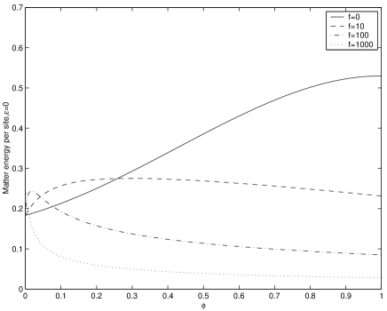
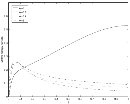
Figure 2: The contribution of $q$ plus ghost fields to the bulk energy. In the left graph we have taken $\epsilon\to 0$ holding $\phi^{\prime}=\epsilon f$ fixed. The right graph is plotted for fixed $\epsilon=0.001$. Note that the effect of finite $\epsilon$ is concentrated near $\phi=0$.

For fixed $\phi,\phi^{\prime}$, both $\alpha$ and $\beta$ are of $O(1/\epsilon)$ as $\epsilon\to 0$. With no relation between them, it is easily seen that the tension is of $O(\sqrt{\epsilon})$ and hence vanishes. If, however the limit can be taken in a way that $(\alpha^{2}-\beta^{2})/\alpha$ is finite, the tension will also be finite. This can be achieved either with both $\mbox{$\langle{\scriptstyle++}\rangle$},\mbox{$\langle{\scriptstyle-+}\rangle$}=O({\epsilon})$ or $\mbox{$\langle{\scriptstyle++}\rangle$}=O(1)$ while $\mbox{$\langle{\scriptstyle-+}\rangle$}=O(\epsilon)$. In the second case, writing $\phi^{\prime}=\epsilon f$ and $\mbox{$\langle{\scriptstyle-+}\rangle$}=\epsilon fG(\phi)$, we find

$$T_{\rm eff}^{\epsilon=0}(\phi,f)={m\over a\sqrt{2(1+fG(\phi))}}\;.$$ (25)

For generic fields the mean field approximation amounts to a string description of the system, with a field dependent tension. But only if $fG(\phi)$ is finite for the field values that minimize the energy, will the system behave like an actual physical string.

The matter contribution to the ground state bulk energy is (see Eq. 186):

$${\cal E}_{m}(\phi,\phi^{\prime})=-{d\over 4}(\xi_{1}+\xi_{2})+{d\over 2M}\sum_{l<M/2}[\xi^{l}_{+}+\xi^{l}_{-}+\ln(\alpha^{2}-\beta^{2})]+{d\over 2}{3\phi+\phi^{\prime}\over 4}\ln(1+\rho)$$

Since the explicit expression is quite complicated, we display this function graphically. In Fig. 2 we show the matter energy as a function of $\phi$ for a sample of $\phi^{\prime}$ values. In these graphs we are assuming the factorization $\mbox{$\langle{\scriptstyle++}\rangle$}=\phi^{2},\mbox{$\langle{\scriptstyle-+}\rangle$}=\phi\phi^{\prime},\mbox{$\langle{\scriptstyle+++}\rangle$}=\phi^{3},\mbox{$\langle{\scriptstyle-++}\rangle$}=\mbox{$\langle{\scriptstyle+-+}\rangle$}=\phi^{2}\phi^{\prime}$. The effect of the infra-red cutoff $\epsilon$ is seen by comparing the case with $\epsilon=0$, $f=\phi^{\prime}/\epsilon$ fixed, to the case with $\epsilon=0.001$, $\phi^{\prime}$ fixed. It clearly has the most dramatic effect in the region of small $\phi$.

\psfrag{Spin energy per site, g}[l][l][.46]{{Spin energy per site, ${\hat{g}}$}}\includegraphics[width=227.62204pt]{articlespinpolygm2.eps}

\psfrag{Spin energy per site, g}[l][l][.46]{{Spin energy per site, ${\hat{g}}$}}\includegraphics[width=227.62204pt]{articlespinpolyg0.eps}

\psfrag{Spin energy per site, g}[l][l][.46]{{Spin energy per site, ${\hat{g}}$}}\includegraphics[width=227.62204pt]{articlespinpolyg2.eps}

\psfrag{Spin energy per site, g}[l][l][.46]{{Spin energy per site, ${\hat{g}}$}}\includegraphics[width=227.62204pt]{articlespinpolyg4.eps}

Figure 3: The contribution of the spin sum to the bulk energy per site using (30), which neglects all short range correlations.

As already mentioned, we present two treatments of the Ising spin contribution to the energy. In the first (simplest but most drastic) option all spin dependence in the action is replaced by its corresponding expectation value, and the spin sum reduces to a trivial independent sum on each site:

$$\prod_{kj}\sum_{P_{k}^{j}=0,1}e^{\kappa_{k}^{j}P_{i}^{j}}=\exp\left\{\sum_{kj}\ln(1+e^{\kappa_{k}^{j}})\right\}.$$ (26)

This version completely neglects short range correlations. Since this represents the entire $\kappa$ dependence of the approximate $W$ the relation of $\phi$ to $\kappa$ is independent on each site:

$$\phi_{k}^{j}={e^{\kappa_{k}^{j}}\over 1+e^{\kappa_{k}^{j}}},\qquad{\rm or}\qquad e^{-\kappa_{k}^{j}}={1\over\phi_{k}^{j}}-1.$$ (27)

Because the spin sum is independent on each site all expectations of the monomials of $P$’s appearing in the action factorize into the corresponding monomials of $\phi$.

We denote by ${\cal A}_{s}$ the spin part of the effective action, including the $-\kappa\phi$ term of the Legendre transform and also the terms involving the coupling constant:

$${\cal A}_{s} = \sum_{kj}\left[-\kappa_{k}^{j}\phi_{k}^{j}+\ln(1+e^{\kappa_{k}^{j}})\right]+2\ln{\hat{g}}\sum_{kj}\langle(P_{k}^{j}(1-P_{k}^{j+1})\rangle$$ (28)

$$\to \sum_{kj}\left[-\phi_{k}^{j}\ln\phi_{k}^{j}-(1-\phi_{k}^{j})\ln(1-\phi_{k}^{j})\right]+\ln{\hat{g}}^{2}\sum_{kj}\phi_{k}^{j}(1-\phi_{k}^{j+1})$$ (30)

$$\to -MN\bigg{\{}{3\over 4}[\phi\ln{\phi}+(1-\phi)\ln(1-\phi)]+{1\over 4}[\phi^{\prime}\ln{\phi^{\prime}}+(1-\phi^{\prime})\ln(1-\phi^{\prime})]$$

$$-{1\over 4}\left({3}\phi+\phi^{\prime}-2\phi\phi^{\prime}-2\phi^{2}\right)\ln{\hat{g}}^{2}\bigg{\}}\equiv-MN{\cal E}_{s}(\phi,\phi^{\prime}),$$

where the last line specializes to the fishnet spin pattern. Since the pattern is regular in the temporal direction the coefficient of $-N$ is just the energy in units of $1/a$ and the coefficient of $-MN$ is the energy per site ${\cal E}_{s}$.

We display the spin energy per site for various couplings in Fig. 3. These graphs display three distinct phases for the spin system. At weak coupling the $\phi^{\prime}=\phi$ curve indicates a degenerate ground state with $\phi\approx 0,1$. These values correspond to the Ising spins aligned with values $-1,+1$ respectively, a ferromagnetic phase. The curves with $\phi^{\prime}$ constrained to $0,0.1,0.2$ approximate the $\phi^{\prime}=\phi$ curve more closely as $\phi^{\prime}\to 0$. At intermediate coupling the minimum of the $\phi^{\prime}=\phi$ curve is fixed at $\phi=1/2$, corresponding to $\langle s_{k}^{j}\rangle=0$ for the Ising spins. This is a disordered phase. The constrained $\phi^{\prime}$ curves give more information about this phase. At ${\hat{g}}^{2}=1$ they all show a minimum for $\phi=1/2$. For ${\hat{g}}^{2}>1$ the minima of these curves are above $1/2$, approaching $1/2$ as $\phi^{\prime}$ increases. In other words the $\phi$ sites are anti-correlated with the $\phi^{\prime}$ sites. This anti-correlation will tend to reduce the paramagnetic susceptibility. For ${\hat{g}}^{2}<1$ (not shown) the curves would have minima less than $1/2$ that all lie on the $\phi^{\prime}=\phi$ curves. In other words the $\phi$ sites are positively correlated with the $\phi^{\prime}$ sites, and this will tend to increase the paramagnetic susceptibility. In summary, although the phase is not ordered, it shows a paramagnetic susceptibility that increases as ${\hat{g}}^{2}$ decreases. Finally for strong coupling the $\phi^{\prime}=\phi$ curve no longer contains the minimum energy. The minimum energy is on the curve with $\phi^{\prime}=0$ at $\phi\approx 0.7$, an anti-ferromagnetic phase. This phase structure is not surprising because the spin energy is essentially the mean field free energy of an Ising model, and the phases we have described are well understood properties of the Ising model provided its dimensionality $d>1$. The mean field description fails to predict the critical exponents for $d=2$.

\psfrag{Spin energy per site, g}[l][l][.46]{{Spin energy per site, ${\hat{g}}$}}\includegraphics[width=227.62204pt]{articlespinnonpolyrevgm2.eps}

\psfrag{Spin energy per site, g}[l][l][.46]{{Spin energy per site, ${\hat{g}}$}}\includegraphics[width=227.62204pt]{articlespinnonpolyrevg0.eps}

\psfrag{Spin energy per site, g}[l][l][.46]{{Spin energy per site, ${\hat{g}}$}}\includegraphics[width=227.62204pt]{articlespinnonpolyrevg2.eps}

\psfrag{Spin energy per site, g}[l][l][.46]{{Spin energy per site, ${\hat{g}}$}}\includegraphics[width=227.62204pt]{articlespinnonpolyrevg4.eps}

Figure 4: The contribution of the spin sum to the bulk energy, using (31) which includes coupling dependence, and hence some temporal correlations, in the spin sum. Note the disappearance of the phase transitions.

However, the spin sums we have actually done correspond to Ising couplings in one dimension only (the temporal direction), and it is well-known that the 1$d$ Ising model displays no phase transitions: there is only a single disordered phase, albeit with paramagnetic properties. In our worldsheet system there are some direct spatial couplings of the spins, and there are also indirect spatial couplings induced through the spin-matter coupling terms. When these spatial couplings are brought into play, a phase transition is no longer ruled out, but it still behooves us to do a better job on the one-dimensional spin sums that removes this artificial phase transition. For that reason we now turn to the more sophisticated treatment of the spin sums sketched in Appendix A. In this better approach the spins multiplying $\ln{\hat{g}}$ are not replaced by mean fields but rather incorporated exactly in the spin sum. However this sum is tractable only after one specializes to a regular spin pattern, here the fishnet spin pattern. Then the problem is solved by finding the eigenvalues of the $2\times 2$ transfer matrix and choosing the largest eigenvalue. In the notation of Appendix A the spin energy per site now becomes

$${\cal E}_{s}=-{1\over 4}\ln t_{+}^{4}(\kappa,\kappa^{\prime})+{1\over 2}\phi\kappa+{1\over 4}K\phi+{1\over 4}\phi^{\prime}\kappa^{\prime}.$$ (31)

Again we display the spin energy in this case graphically in Fig. 4. We see that the indications of a phase transition seen in Fig. 3 have now disappeared, since we now have an essentially exact treatment of the 1$d$ Ising model reflected in the spin sum. Now the minimum energy is always on the $\phi^{\prime}=\phi$ curve and located at $\phi=1/2$, the disordered phase. But the $\phi^{\prime}\neq\phi$ curves still show that this phase is paramagnetic: for ${\hat{g}}^{2}<1$ the susceptibility is greater than in the disordered phase and it is less for ${\hat{g}}^{2}>1$. We shall see that these qualitative features are maintained when we add in the energy of the matter sector. The $\phi^{\prime}=0$ curve follows the fate of the fishnet diagram, corresponding to the endpoint $\phi=1$, when the rest of the planar diagrams are included. In the following analysis we shall always display plots for the total energy per site in this second more accurate treatment of the spin sum.

\psfrag{Total energy per site, g}[l][l][.45]{{Total energy per site, ${\hat{g}}$}}\includegraphics[width=227.62204pt]{article1gm2corr.eps}

\psfrag{Total energy per site, g}[l][l][.45]{{Total energy per site, ${\hat{g}}$}}\includegraphics[width=227.62204pt]{article1g0corr.eps}

\psfrag{Total energy per site, g}[l][l][.45]{{Total energy per site, ${\hat{g}}$}}\includegraphics[width=227.62204pt]{article1g2corr.eps}

\psfrag{Total energy per site, g}[l][l][.45]{{Total energy per site, ${\hat{g}}$}}\includegraphics[width=227.62204pt]{article1g4corr.eps}

Figure 5: The total energy for $\epsilon=1$. The location of the minimum depends dramatically on the coupling.

\psfrag{Total energy per site, g}[l][l][.45]{{Total energy per site, ${\hat{g}}$}}\includegraphics[width=227.62204pt]{article000001gm2corr.eps}

\psfrag{Total energy per site, g}[l][l][.45]{{Total energy per site, ${\hat{g}}$}}\includegraphics[width=227.62204pt]{article000001g0corr.eps}

\psfrag{Total energy per site, g}[l][l][.45]{{Total energy per site, ${\hat{g}}$}}\includegraphics[width=227.62204pt]{article000001g2corr.eps}

\psfrag{Total energy per site, g}[l][l][.45]{{Total energy per site, ${\hat{g}}$}}\includegraphics[width=227.62204pt]{article000001g4corr.eps}

Figure 6: The total energy for $\epsilon=0.00001$, corresponding to a very small infra-red cutoff (very large transverse space). The location of the absolute minimum is at $\phi=0.5$ for all coupling, but the paramagnetic properties of the spins show a clear dependence on the coupling.

\psfrag{Total energy per site, g}[l][l][.45]{{Total energy per site, ${\hat{g}}$}}\includegraphics[width=227.62204pt]{article000001gm2rho1lin.eps}

\psfrag{Total energy per site, g}[l][l][.45]{{Total energy per site, ${\hat{g}}$}}\includegraphics[width=227.62204pt]{article000001gm1rho1lin.eps}

\psfrag{Total energy per site, g}[l][l][.45]{{Total energy per site, ${\hat{g}}$}}\includegraphics[width=227.62204pt]{article000001g0rho1lin.eps}

\psfrag{Total energy per site, g}[l][l][.45]{{Total energy per site, ${\hat{g}}$}}\includegraphics[width=227.62204pt]{article000001g2rho1lin.eps}

Figure 7: The total energy for the massive case, $\rho=1$, $\epsilon=0.00001$. There is evidence for ferromagnetic behavior at weak coupling but none for anti-ferromagnetic behavior at strong coupling. Note the qualitative similarity of these curves to those of Fig. 5.

\psfrag{Total energy per site, g}[l][l][.45]{{Total energy per site, ${\hat{g}}$}}\includegraphics[width=227.62204pt]{article0gm2corr.eps}

\psfrag{Total energy per site, g}[l][l][.45]{{Total energy per site, ${\hat{g}}$}}\includegraphics[width=227.62204pt]{article0g0corr.eps}

\psfrag{Total energy per site, g}[l][l][.45]{{Total energy per site, ${\hat{g}}$}}\includegraphics[width=227.62204pt]{article0g2corr.eps}

\psfrag{Total energy per site, g}[l][l][.45]{{Total energy per site, ${\hat{g}}$}}\includegraphics[width=227.62204pt]{article0g4corr.eps}

Figure 8: The total energy for $\epsilon=0$ for fixed $f=\phi^{\prime}/\epsilon$.

\psfrag{g}[l][l][.5]{${\hat{g}}$}\includegraphics[width=227.62204pt]{article0tensioncorr.eps}

\psfrag{g}[l][l][.5]{${\hat{g}}$}\includegraphics[width=227.62204pt]{article0emincorr.eps}

Figure 9: String tension on the left and minimum energy on the right as functions of $f=\phi^{\prime}/\epsilon$ with $\epsilon\to 0$. The monotonic decrease in both curves indicates the vanishing of string tension in the ground state.

We now come to the total energy. The details of the matter contribution to the energy are contained in Appendix C. For ease of comparison we shall display graphs for the same parameters we chose in the spin energy. We start by displaying the total energy curves for $\epsilon=1$ so that the infra-red cutoff in transverse space is $L\sim O(\sqrt{a/m})$. These results are shown in Fig. 5. We first note that as with the spin energy, it is still true that the lowest energy solution always falls on the $\phi=\phi^{\prime}$ curve, and there is no indication of a phase transition. However, the location of the minimum now depends dramatically on the value of ${\hat{g}}^{2}$. It evidently approaches $\phi=0$ for weak coupling and $\phi=1/2$ for strong coupling. Looking at the $\phi^{\prime}=0$ curves we see first that the fishnet diagram $\phi=1$ on this curve predicts positive energy for weak and intermediate coupling. By ${\hat{g}}^{2}=100$ this diagram predicts negative energy. But in all cases the minimum of the $\phi^{\prime}=0$ curve is negative but higher in energy than the uniform $\phi^{\prime}=\phi$ case.

Next we display graphs with $\epsilon=0.00001$ and the same range of couplings. We see from Fig 6 that qualitatively the energy curves resemble more closely those of the spin energy alone. The minimum energy again lies on the $\phi^{\prime}=\phi$ curve and is located at $\phi=1/2$ for all couplings. And again we see the same paramagnetic tendencies in the fixed $\phi^{\prime}$ curves for strong and weak coupling. The string tension for this lowest energy state can be found explicitly. Since $\phi=\phi^{\prime}=1/2$ at this point, it follows that $\kappa=0$ so $\mbox{$\langle{\scriptstyle++}\rangle$}=\mbox{$\langle{\scriptstyle-+}\rangle$}=\phi/t_{+}(0)=1/(2+2{\hat{g}})$. Thus

$$T_{\rm eff}={m\over a}\sqrt{2\epsilon(1+{\hat{g}})},$$ (32)

which vanishes for $\epsilon\to 0$ at fixed ${\hat{g}}$. Vanishing tension implies among other things a gapless energy spectrum.

In Fig. 7 we display the energy curves for a massive scalar field. It is interesting that, for weak coupling, there are indications of a ferromagnetic behavior. (We were able to do calculations at zero mass because of our cutoffs.) Notice though that for ${\hat{g}}^{2}>1$ the massive case is very similar to the massless case. In particular, at strong coupling we see a continuous approach to the disordered phase $\phi=1/2$ and no anti-ferromagnetic behavior. Notice that although there are quantitative differences, the energy curves for the massive case at $\epsilon=.00001$ are qualitatively similar to those of the massless case at $\epsilon=1$. This is perhaps reasonable because both $\rho=1$ and $\epsilon=1$ set an infra-red cutoff of the same order of magnitude $L^{2}=O(a/m)$.

${\hat{g}}^{2}$	$\rho$	$\epsilon$	${\cal E}_{min}$	$\phi_{min}$	$\kappa_{min}$	$\langle{\scriptstyle++}\rangle$	$\langle{\scriptstyle+++}\rangle$	${a\over m}T_{\rm eff}$
.01	0	1	-.0651	0.0208	-.6598	.0106	.0054	9.713
.01	0	$10^{-5}$	-.0893	.5	0	.4545	.4132	.00492
.01	1	$10^{-5}$	.0176	0.0531	-.3959	.0351	.0232	.0169
.1	1	$10^{-5}$	-0.0663	0.1527	-.6015	.0761	.0379	.0115
1	0	1	-.4860	.1680	-1.6000	.0282	.0047	5.955
1	0	$10^{-5}$	-.6850	.5	0	.250	.125	.00632
1	1	$10^{-5}$	-.3931	0.3543	-.6000	.1256	.0445	.00892
100	0	1	-2.208	.4380	-2.049	.0132	3.95$\cdot 10^{-4}$	8.704
100	0	$10^{-5}$	-2.3792	.5	0	.0455	.0041	.01482
100	1	$10^{-5}$	-2.0353	0.4895	-.4189	.0360	.0026	.0167
$10^{4}$	0	1	-4.501	.4892	-3.031	.001	2.25$\cdot 10^{-6}$	31.62
$10^{4}$	0	$10^{-5}$	-4.574	.505	1.8189	.0124	3.03$\cdot 10^{-4}$	.0284

Table 1: The worldsheet parameters for ${\rm Tr}\Phi^{3}$ theory, fixed by minimizing the energy in the mean field approximation.

Let us now consider what these calculations tell us about the role of the fishnet diagram. We can follow the fate of the fishnet diagram in two stages. Starting at $\phi^{\prime}=0,\phi=1$ we first let $\phi$ relax at fixed $\phi^{\prime}=0$ to the minimum energy at $\phi^{\prime}=0$. Since $\mbox{$\langle{\scriptstyle-+}\rangle$}=0$, the string tension along this curve is $(m/a)\sqrt{(1+4\epsilon/\mbox{$\langle{\scriptstyle++}\rangle$})/2}$, which is simply $m/(a\sqrt{2})$ as $\epsilon\to 0$. Then one can begin to relax $\phi^{\prime}$ putting $\phi^{\prime}=\epsilon f$. Then one can smoothly send $\epsilon$ to zero at fixed $f$, and study how the physics evolves as $f$ increases. The field dependence of the energy is shown in Fig. 8. One should keep in mind that because of our limiting procedure all these curves are infinitesimally near the $\phi^{\prime}=0$ curves of the previous graphs. In Fig. 9 we show the string tension corresponding to the minimal point on each fixed $f$ curve as a function of $f$. Next to it we display the corresponding minimal energy as a function of $f$. We see that both string tension and energy generally decrease as $f$ increases. Note, however that a small energy barrier between $f=0$ and $f>10$ is visible on the ${\hat{g}}^{2}=.01$ curve. Although not visible there are similar tinier barriers at higher coupling. It is clear from the previous graphs that the general decreasing trend continues till infinite $f$ where the tension goes to zero and the energy reaches its minimum. Our conclusion is that, for ${\rm Tr}\Phi^{3}$ theory, the fishnet phase is not stable and though there is a stringy description for generic values of the fields, the system relaxes to a ground state with no mass gap and zero string tension. In the table we have compiled a list of the relevant parameters characterizing the physics of this global minimum for various $\hat{g},\rho,\epsilon$.

What would we expect to happen in a theory like QCD which ought to confine quarks by forming stringy flux tubes? The failure of the ${\rm Tr}\Phi^{3}$ theory to form string isn’t just signified by the monotonic decrease of effective tension with $f$, but rather with the correlation of this behavior with the monotonic decrease of the associated system energy. If the system energy had a minimum at finite $f$, its ground state would support a non-vanishing string tension at the corresponding $f$. This is what we should expect to happen for QCD and other confining theories. Moreover, for QCD this should occur for couplings of $O(1)$.

5 Mean Field Treatment of the Matter Fields (Large $d=D-2$)

In the previous section we built the mean field approximation on the mean field $\phi=\langle P\rangle$ representing the average value of the Ising spin, following [7]. But another, perhaps superior, approach is to instead focus on a mean field defined as the average value of an $SO(d)$ scalar bilinear of the matter fields, as suggested in [8]. (Such a description should be accurate in the parametric limit $d\to\infty$. The existence of this parametric limit in which the approximation is good is a significant virtue of this approach, although the underlying field theories we are describing are only meaningful in sufficiently low dimensions.) In this approach we want our mean field to be an order parameter which measures the presence of an effective string tension, so it is natural to define

$$\chi_{k}^{j}\equiv-{a\over m\epsilon}\left\langle{1\over 2}({\boldsymbol{q}}_{k}^{j}-{\boldsymbol{q}}_{k}^{j-1})^{2}-{\boldsymbol{b}}_{k}^{j}{\boldsymbol{c}}_{k}^{j}\right\rangle.$$ (33)

Accordingly, we add a source term to the worldsheet action

$$-{a\over m\epsilon}\sum_{kj}J_{k}^{j}\left[{1\over 2}({\boldsymbol{q}}_{k}^{j}-{\boldsymbol{q}}_{k}^{j-1})^{2}-{\boldsymbol{b}}_{k}^{j}{\boldsymbol{c}}_{k}^{j}\right].$$ (34)

The path integral in the presence of $J$ is defined to be $e^{W(J)}$, the field is then $\chi_{k}^{j}=\partial W/\partial J_{k}^{j}$, and the effective action is given by

$${\cal A}\equiv W-\sum_{kj}\chi_{k}^{j}J_{k}^{j}.$$ (35)

The mean field approximation is then implemented by establishing the relation between $\chi$ and $J$ as that arising from the path integral over matter fields neglecting the terms in the action that couple the matter to the Ising spins. In other words we take the $J$ dependence of $W$ to be that of $W_{m}$ defined by

$$e^{W_{m}(J)} \equiv \int DcDbD{\boldsymbol{q}}\exp\left\{-{a\over 2m}\sum_{k,j}{({\boldsymbol{q}}_{k+1}^{j}-{\boldsymbol{q}}_{k}^{j})^{2}}-{a\over 2m\epsilon}\sum_{k,j}{J}_{k}^{j}{({\boldsymbol{q}}_{k}^{j}-{\boldsymbol{q}}_{k}^{j-1})^{2}}+{a\over m\epsilon}\sum_{k,j}{J}_{k}^{j}{\boldsymbol{b}}^{j}_{k}{\boldsymbol{c}}^{j}_{k}\right\}$$ (36)

$$\exp\left\{{a\over m}\sum_{k,j}({\boldsymbol{b}}_{k+1}^{j}-{\boldsymbol{b}}_{k}^{j})({\boldsymbol{c}}_{k+1}^{j}-{\boldsymbol{c}}_{k}^{j})\right\}$$

We then use this approximate path integral to approximate the matter dependence of the terms in the action coupling to the Ising spins by their average values. In practice we assume that $J$ (and hence also $\chi$) is uniform in $k,j$. Then by consulting Appendix C, we find that

$$W_{m}(J) = -MN\left[{2d\over\pi}{\rm Re}\left\{i{\rm Li}_{2}\left({1\over i}\sqrt{\epsilon\over J}\right)\right\}-d\ln\left({1\over 2}+\sqrt{{1\over 4}+{\epsilon\over J}}\right)\right]$$ (37)

$$-{a\over m\epsilon}\left\langle{1\over 2}({\boldsymbol{q}}_{k}^{j}-{\boldsymbol{q}}_{k}^{j-1})^{2}-{\boldsymbol{b}}_{k}^{j}{\boldsymbol{c}}_{k}^{j}\right\rangle = {1\over MN}{\partial W_{m}\over\partial J}=\chi(J)$$ (38)

$${a\over m}\left\langle{\boldsymbol{b}}_{k}^{j}{\boldsymbol{c}}_{k}^{j}\right\rangle = {d\over 2}{a\over m}\left\langle{b}_{k}^{j}{c}_{k}^{j}\right\rangle={d\epsilon\over 2\sqrt{J^{2}+4\epsilon J}}$$ (39)

$${a\over m}\left\langle({\boldsymbol{b}}_{k+1}^{j}-{\boldsymbol{b}}_{k}^{j})({\boldsymbol{c}}_{k+1}^{j}-{\boldsymbol{c}}_{k}^{j})\right\rangle = {d\over 2}{a\over m}\left\langle({b}_{k+1}^{j}-{b}_{k}^{j})({c}_{k+1}^{j}-{c}_{k}^{j})\right\rangle={d\over 2}\left[1-{J\over\sqrt{J^{2}+4\epsilon J}}\right].$$ (40)

Inserting these results into the summand for the spin sum, we find that the spin sum is just a two dimensional generalized Ising model with Boltzmann factor $e^{A(P)}$ with

$$A(P) = \ln{\hat{g}}\sum_{kj}{1-s_{k}^{j}s_{k}^{j-1}\over 2}-{d\over 2}\ln\left(1+\rho\right)\sum_{k,j}P_{k}^{j}+{\chi(J)}\sum_{kj}P_{k}^{j}P_{k}^{j-1}$$ (41)

$$+\sum_{kj}\left\{{\epsilon\over\sqrt{J^{2}+4\epsilon J}}\left[{d\over 2}A^{\prime}_{kj}-B_{k}^{j}\right]+\left[1-{J\over\sqrt{J^{2}+4\epsilon J}}\right]\left[{d\over 2}C^{\prime}_{kj}-D_{k}^{j}\right]\right\}$$

$$A^{\prime}_{kj} = {P}_{k}^{j+1}{P}_{k}^{j}-{P}_{k}^{j-1}{P}_{k}^{j}{P}_{k}^{j+1}+(1-P_{k}^{j})(P_{k+1}^{j}+P_{k-1}^{j})+\rho(1-P_{k}^{j})P_{k-1}^{j-1}P_{k-1}^{j}$$ (42)

$$C^{\prime}_{kj} = (1-P_{k}^{j})(1-P_{k+1}^{j})-1=P_{k}^{j}P_{k+1}^{j}-P_{k}^{j}-P_{k+1}^{j}$$ (43)

and $B$ and $D$ are unchanged. Defining $e^{W_{s}(J)}=\sum_{P=0,1}e^{A}$, the total effective action is

$${\cal A}\approx W_{m}(J)+W_{s}(J)-MNJ\chi(J).$$ (44)

and the value of $J$ (or of $\chi(J)$) is determined as a stationary point of ${\cal A}$ that minimizes the energy per site ${\cal E}=-{\cal A}/MN$. To calculate $W_{s}$ with no further approximation we would need the exact solution of the two dimensional spin system defined by (41). This system differs from the soluble two dimensional Ising model by linear terms in the spins (a constant magnetic field) and also higher than quadratic terms in the spin. For generic $J$ and coupling parameters this model certainly has no analytic solution. A numerical solution can be attempted, but we leave this problem for future research.

Instead we note that, in this setup, the mean field $\chi$ acts as a source for the spin bilinear $\langle P_{k}^{j}P_{k}^{j-1}\rangle$, and so its conjugate $J$ is in this sense a mean field for this bilinear. Thus a natural mean field approach to the two dimensional Ising system encountered here is to use $\varphi_{k}^{j}\equiv\langle P_{k}^{j}P_{k}^{j-1}\rangle$ as the mean field. But once we treat the Ising spins in this way, nothing is really gained by introducing a source for the matter bilinears, and so we will only source the spin bilinear, repeating the mean field treatment of the previous section using this new order parameter. In the rest of this section we describe the results of doing this, and we compare them to those of the more traditional mean field treatment of the previous section. Although this second study will not be different in spirit from that of the previous section, it will give us some idea of the robustness of the mean field method.

We introduce the source by inserting $e^{\sum\chi_{k}^{j}P_{k}^{j}P_{k}^{j-1}}$ into the original path integral (2), and we define $W(\chi)$ by calling the resulting path integral $e^{W}$. Then our effective field is $\varphi_{k}^{j}=\partial W/\partial\chi_{k}^{j}$ and the effective action is

$${\cal A}(\varphi)=W(\chi)-\sum_{kj}\varphi_{k}^{j}\chi_{k}^{j}.$$ (45)

As in Section 4 we define the mean field approximation by doing the spin sum with the spin dependent terms in the matter action fixed to their expectation values which are then self-consistently determined. In contrast to section 4, the mean fields here are the bilinears $\langle P_{k}^{j-1}P_{k}^{j}\rangle$ and the derived expectations are now the linear and cubic ones $\langle P_{k}^{j}\rangle$ and $\langle P_{k}^{j-1}P_{k}^{j}P_{k}^{j+1}\rangle$.

For the fishnet spin pattern $\varphi_{k}^{j}=\varphi,\varphi,\varphi^{\prime},\varphi^{\prime},\varphi,\varphi,\ldots$, there are three distinct values each for the linear and cubic cases. As explained in Appendix A.2, where these expectations are evaluated, we denote the linear ones by $\phi,\phi^{\prime}$, and ${\tilde{\phi}}$ and the cubic ones by $\langle{\scriptstyle+++}\rangle$, $\langle{\scriptstyle-++}\rangle$, and $\langle{\scriptstyle+-+}\rangle$. The matter integrals are evaluated in Appendix C.2, basically by substituting a new set of coefficients for the $\alpha,\beta,\gamma,\delta$ coefficients of C.1. Now the effective string tension depends directly on the background fields

$$T_{\rm eff}=\frac{m}{a}\sqrt{\frac{(4\epsilon+\varphi+\varphi^{\prime})}{2(\varphi+\varphi^{\prime})+\varphi\varphi^{\prime}/\epsilon)}}.$$ (46)

As before the tension goes to zero as $\epsilon\to 0$ unless $\varphi^{\prime}={\cal O}(\epsilon)$.

\psfrag{varphi}[l][l][.55]{$\varphi$}\psfrag{phi^prime = phi}[l][l][.55]{$\varphi^{\prime}=\varphi$}\psfrag{phi^prime = 0.1}[l][l][.55]{$\varphi^{\prime}=0.1$}\psfrag{phi^prime = 0.2}[l][l][.55]{$\varphi^{\prime}=0.2$}\psfrag{phi^prime = 0.3}[l][l][.55]{$\varphi^{\prime}=0.3$}\psfrag{phi^prime = 0}[l][l][.55]{$\hskip-6.7pt\varphi^{\prime}=0$}\psfrag{Spin energy per site}[l][l][.55]{Spin energy per site}\psfrag{g^2=100, \epsilon=10^(-5), \rho=0}[l][l][.55]{$\hat{g}^{2}=0.01,\epsilon=10^{-5},\rho=0$}\psfrag{g}[l][l][.46]{${\hat{g}}$}\includegraphics[width=227.62204pt,height=156.49014pt]{articlespinvspp000001g0.eps}

\psfrag{varphi}[l][l][.55]{$\varphi$}\psfrag{phi^prime = phi}[l][l][.55]{$\varphi^{\prime}=\varphi$}\psfrag{phi^prime = 0.1}[l][l][.55]{$\varphi^{\prime}=0.1$}\psfrag{phi^prime = 0.2}[l][l][.55]{$\varphi^{\prime}=0.2$}\psfrag{phi^prime = 0.3}[l][l][.55]{$\varphi^{\prime}=0.3$}\psfrag{phi^prime = 0}[l][l][.55]{$\hskip-6.7pt\varphi^{\prime}=0$}\psfrag{Spin energy per site}[l][l][.55]{Spin energy per site}\psfrag{g^2=100, \epsilon=10^(-5), \rho=0}[l][l][.55]{$\hat{g}^{2}=0.01,\epsilon=10^{-5},\rho=0$}\psfrag{g}[l][l][.46]{${\hat{g}}$}\psfrag{g^2=1,epsilon=10^(-5),rho=0}[l][l][.55]{$\hat{g}^{2}=1,\epsilon=10^{-5},\rho=0$}\includegraphics[width=227.62204pt]{spineng1e10m5nomassPPgen.eps}

Figure 10: The spin energy per site for the massless case, $\rho=0$, $\epsilon=10^{-5}$. On the left are the $\hat{g}^{2}=1$ spin energy curves from Fig. 4 plotted versus $\langle{\scriptstyle++}\rangle$. On the right are the analogous curves from the mean field treatment of Section 5.

The energy function ${\cal E}(\varphi,\varphi^{\prime})$ is certainly a different function of its two variables than the energy function of Section 4, both because the variables are differently defined and because the different structure of the source terms leads to an effectively different treatment of fluctuation effects in the corresponding mean field approximations. To display these differences graphically we choose a typical coupling ${\hat{g}}^{2}=1$ for which they are evident. In Fig. 10 we show on the left the spin energy curves for this case from Fig. 4 in Section 4, replotted as a function of $\langle{\scriptstyle++}\rangle$, the physical quantity measured by $\varphi$. On the right we show the corresponding curves from the treatment of this section as functions of $\varphi$. The most dramatic difference compared to Fig. 4 is the move of the location of the minimum energy toward the origin. This effect is clearly accounted for by the change of independent variables from $\phi$ to $\langle{\scriptstyle++}\rangle$. Next the shape of the curves on the left is slightly different in detail than those on the right, but the ordering of the curves is the same in both figures in the region near the minimum. Note that the $\phi=\phi^{\prime}$ ($\varphi=\varphi^{\prime}$) curves in the left and right are essentially identical. However there is a significant lowering in energy of the constrained curves on the right compared to those on the left. This quantitative difference in the mean field treatments is reasonable considering that the constraints imposed on bilinears $\varphi,\varphi^{\prime}$ in the present section are less severe than the constraints imposed on $\phi^{\prime}$ in Section 4. Hence the constrained system in the former case should be closer to the unconstrained ground state and the corresponding energies should be lower. Also the slicing of the two dimensional surfaces is slightly different in the two cases. This interpretation is supported by the fact that the ground state curve is not significantly altered. These two differences, the move toward the origin, and the lowering in energy of the constrained curves but not of the ground state curves are present in the spin energy for other couplings, but there are no other significant differences, so we don’t display all those cases.

Finally we turn our attention to the total energy per site. In Fig. 11 we display the total energy curves for the massless case and the same set of couplings used in Section 4. These graphs should be compared to Fig. 6. The most dramatic apparent difference is the movement of the minimum toward the origin as the coupling increases. As discussed in the previous paragraph, this is explained by the change of independent variables from $\phi$ to $\langle{\scriptstyle++}\rangle$. For the strongest coupling displayed the minimum is for $\varphi\approx.01$. We also see the trend that the constrained curves generally lie lower in energy in Fig. 11 than in Fig. 6. But note that these constrained curves are not really comparable at strong coupling because in Fig. 11 most of the $\varphi^{\prime}$ choices are larger than the location of the minimum, in contrast to Fig. 6 where all of the $\phi^{\prime}$ choices are smaller than the location of the minimum. From Fig. 11, we see that the minimum energy is on the $\varphi=\varphi^{\prime}$ curve and the location of this minimum point depends upon the value of $\hat{g}^{2}$. For weak coupling, the minimum point tends to $\varphi=0.5$ and it approaches $\varphi=0$ for strong coupling.

\psfrag{varphi}[l][l][.55]{$\varphi$}\psfrag{phi^prime = phi}[l][l][.55]{$\varphi^{\prime}=\varphi$}\psfrag{phi^prime = 0.1}[l][l][.55]{$\varphi^{\prime}=0.1$}\psfrag{phi^prime = 0.2}[l][l][.55]{$\varphi^{\prime}=0.2$}\psfrag{phi^prime = 0.3}[l][l][.55]{$\varphi^{\prime}=0.3$}\psfrag{phi^prime = 0}[l][l][.55]{$\hskip-6.7pt\varphi^{\prime}=0$}\psfrag{Total energy per site}[l][l][.55]{Total energy per site}\psfrag{g^2=0.01,epsilon=10^(-5),rho = 0}[l][l][.55]{$\hat{g}^{2}=0.01,\epsilon=10^{-5},\rho=0$}\includegraphics[width=227.62204pt]{toteng001e10m5nomassPP.eps}

\psfrag{varphi}[l][l][.55]{$\varphi$}\psfrag{phi^prime = phi}[l][l][.55]{$\varphi^{\prime}=\varphi$}\psfrag{phi^prime = 0.1}[l][l][.55]{$\varphi^{\prime}=0.1$}\psfrag{phi^prime = 0.2}[l][l][.55]{$\varphi^{\prime}=0.2$}\psfrag{phi^prime = 0.3}[l][l][.55]{$\varphi^{\prime}=0.3$}\psfrag{phi^prime = 0}[l][l][.55]{$\hskip-6.7pt\varphi^{\prime}=0$}\psfrag{Total energy per site}[l][l][.55]{Total energy per site}\psfrag{g^2=0.01,epsilon=10^(-5),rho = 0}[l][l][.55]{$\hat{g}^{2}=0.01,\epsilon=10^{-5},\rho=0$}\psfrag{varphi}[l][l][.55]{$\varphi$}\psfrag{Total energy per site}[l][l][.55]{Total energy per site}\psfrag{g^2=1,epsilon=10^(-5),rho = 0}[l][l][.55]{$\hat{g}^{2}=1,\epsilon=10^{-5},\rho=0$}\includegraphics[width=227.62204pt]{toteng1e10m5nomassPP.eps}

\psfrag{varphi}[l][l][.55]{$\varphi$}\psfrag{phi^prime = phi}[l][l][.55]{$\varphi^{\prime}=\varphi$}\psfrag{phi^prime = 0.1}[l][l][.55]{$\varphi^{\prime}=0.1$}\psfrag{phi^prime = 0.2}[l][l][.55]{$\varphi^{\prime}=0.2$}\psfrag{phi^prime = 0.3}[l][l][.55]{$\varphi^{\prime}=0.3$}\psfrag{phi^prime = 0}[l][l][.55]{$\hskip-6.7pt\varphi^{\prime}=0$}\psfrag{Total energy per site}[l][l][.55]{Total energy per site}\psfrag{g^2=0.01,epsilon=10^(-5),rho = 0}[l][l][.55]{$\hat{g}^{2}=0.01,\epsilon=10^{-5},\rho=0$}\psfrag{varphi}[l][l][.55]{$\varphi$}\psfrag{Total energy per site}[l][l][.55]{Total energy per site}\psfrag{g^2=1,epsilon=10^(-5),rho = 0}[l][l][.55]{$\hat{g}^{2}=1,\epsilon=10^{-5},\rho=0$}\psfrag{Total energy per site}[l][l][.55]{Total energy per site}\psfrag{g^2=100,epsilon=10^(-5),rho = 0}[l][l][.55]{$\hat{g}^{2}=100,\epsilon=10^{-5},\rho=0$}\includegraphics[width=227.62204pt]{toteng100e10m5nomassPP.eps}

\psfrag{varphi}[l][l][.55]{$\varphi$}\psfrag{phi^prime = phi}[l][l][.55]{$\varphi^{\prime}=\varphi$}\psfrag{phi^prime = 0.1}[l][l][.55]{$\varphi^{\prime}=0.1$}\psfrag{phi^prime = 0.2}[l][l][.55]{$\varphi^{\prime}=0.2$}\psfrag{phi^prime = 0.3}[l][l][.55]{$\varphi^{\prime}=0.3$}\psfrag{phi^prime = 0}[l][l][.55]{$\hskip-6.7pt\varphi^{\prime}=0$}\psfrag{Total energy per site}[l][l][.55]{Total energy per site}\psfrag{g^2=0.01,epsilon=10^(-5),rho = 0}[l][l][.55]{$\hat{g}^{2}=0.01,\epsilon=10^{-5},\rho=0$}\psfrag{varphi}[l][l][.55]{$\varphi$}\psfrag{Total energy per site}[l][l][.55]{Total energy per site}\psfrag{g^2=1,epsilon=10^(-5),rho = 0}[l][l][.55]{$\hat{g}^{2}=1,\epsilon=10^{-5},\rho=0$}\psfrag{Total energy per site}[l][l][.55]{Total energy per site}\psfrag{g^2=100,epsilon=10^(-5),rho = 0}[l][l][.55]{$\hat{g}^{2}=100,\epsilon=10^{-5},\rho=0$}\psfrag{varphi}[l][l][.55]{$\varphi$}\psfrag{Total energy per site}[l][l][.55]{Total energy per site}\psfrag{g^2=10^4,epsilon=10^(-5),rho = 0}[l][l][.55]{$\hat{g}^{2}=10^{4},\epsilon=10^{-5},\rho=0$}\includegraphics[width=227.62204pt]{toteng104e10m5nomassPP.eps}

Figure 11: The total energy per site for the massless case, $\rho=0$, $\epsilon=10^{-5}$.

The massive case $\rho=1$ is presented in Fig. 12 and should be compared to Fig. 7. In the latter the location of the minimum is near $\phi=0$ at weak coupling and approaches $\phi=0.5$ at strong coupling. In contrast in Fig. 12, again because of the different variables chosen, the minimum approaches $\varphi=0$ in the strong coupling limit in addition to the weak coupling limit. But the behavior of the constrained curves reflects the qualitatively different physics of the two limits. There is ferromagnetic behavior at weak coupling, with $\varphi$ strongly correlated with $\varphi^{\prime}$. At strong coupling there is very little if any such correlation.

\psfrag{varphi}[l][l][.55]{$\varphi$}\psfrag{phi^prime = phi}[l][l][.55]{$\varphi^{\prime}=\varphi$}\psfrag{phi^prime = 0.1}[l][l][.55]{$\varphi^{\prime}=0.1$}\psfrag{phi^prime = 0.2}[l][l][.55]{$\varphi^{\prime}=0.2$}\psfrag{phi^prime = 0.3}[l][l][.55]{$\varphi^{\prime}=0.3$}\psfrag{phi^prime = 0}[l][l][.55]{$\hskip-6.7pt\phi^{\prime}=0$}\psfrag{Total energy per site}[l][l][.55]{Total energy per site}\psfrag{g^2=0.01,epsilon=10^(-5),rho = 1}[l][l][.55]{$\hat{g}^{2}=0.01,\epsilon=10^{-5},\rho=1$}\includegraphics[width=227.62204pt]{toteng001e10m5massPP.eps}

\psfrag{varphi}[l][l][.55]{$\varphi$}\psfrag{phi^prime = phi}[l][l][.55]{$\varphi^{\prime}=\varphi$}\psfrag{phi^prime = 0.1}[l][l][.55]{$\varphi^{\prime}=0.1$}\psfrag{phi^prime = 0.2}[l][l][.55]{$\varphi^{\prime}=0.2$}\psfrag{phi^prime = 0.3}[l][l][.55]{$\varphi^{\prime}=0.3$}\psfrag{phi^prime = 0}[l][l][.55]{$\hskip-6.7pt\phi^{\prime}=0$}\psfrag{Total energy per site}[l][l][.55]{Total energy per site}\psfrag{g^2=0.01,epsilon=10^(-5),rho = 1}[l][l][.55]{$\hat{g}^{2}=0.01,\epsilon=10^{-5},\rho=1$}\psfrag{Total energy per site}[l][l][.55]{Total energy per site}\psfrag{g^2=1,epsilon=10^(-5),rho = 1}[l][l][.55]{$\hat{g}^{2}=1,\epsilon=10^{-5},\rho=1$}\includegraphics[width=227.62204pt]{toteng1e10m5massPP.eps}

\psfrag{varphi}[l][l][.55]{$\varphi$}\psfrag{phi^prime = phi}[l][l][.55]{$\varphi^{\prime}=\varphi$}\psfrag{phi^prime = 0.1}[l][l][.55]{$\varphi^{\prime}=0.1$}\psfrag{phi^prime = 0.2}[l][l][.55]{$\varphi^{\prime}=0.2$}\psfrag{phi^prime = 0.3}[l][l][.55]{$\varphi^{\prime}=0.3$}\psfrag{phi^prime = 0}[l][l][.55]{$\hskip-6.7pt\phi^{\prime}=0$}\psfrag{Total energy per site}[l][l][.55]{Total energy per site}\psfrag{g^2=0.01,epsilon=10^(-5),rho = 1}[l][l][.55]{$\hat{g}^{2}=0.01,\epsilon=10^{-5},\rho=1$}\psfrag{Total energy per site}[l][l][.55]{Total energy per site}\psfrag{g^2=1,epsilon=10^(-5),rho = 1}[l][l][.55]{$\hat{g}^{2}=1,\epsilon=10^{-5},\rho=1$}\psfrag{Total energy per site}[l][l][.55]{Total energy per site}\psfrag{g^2=100,epsilon=10^(-5),rho = 1}[l][l][.55]{$\hat{g}^{2}=100,\epsilon=10^{-5},\rho=1$}\includegraphics[width=227.62204pt]{toteng100e10m5massPP.eps}

\psfrag{varphi}[l][l][.55]{$\varphi$}\psfrag{phi^prime = phi}[l][l][.55]{$\varphi^{\prime}=\varphi$}\psfrag{phi^prime = 0.1}[l][l][.55]{$\varphi^{\prime}=0.1$}\psfrag{phi^prime = 0.2}[l][l][.55]{$\varphi^{\prime}=0.2$}\psfrag{phi^prime = 0.3}[l][l][.55]{$\varphi^{\prime}=0.3$}\psfrag{phi^prime = 0}[l][l][.55]{$\hskip-6.7pt\phi^{\prime}=0$}\psfrag{Total energy per site}[l][l][.55]{Total energy per site}\psfrag{g^2=0.01,epsilon=10^(-5),rho = 1}[l][l][.55]{$\hat{g}^{2}=0.01,\epsilon=10^{-5},\rho=1$}\psfrag{Total energy per site}[l][l][.55]{Total energy per site}\psfrag{g^2=1,epsilon=10^(-5),rho = 1}[l][l][.55]{$\hat{g}^{2}=1,\epsilon=10^{-5},\rho=1$}\psfrag{Total energy per site}[l][l][.55]{Total energy per site}\psfrag{g^2=100,epsilon=10^(-5),rho = 1}[l][l][.55]{$\hat{g}^{2}=100,\epsilon=10^{-5},\rho=1$}\psfrag{Total energy per site}[l][l][.55]{Total energy per site}\psfrag{g^2=10^4,epsilon=10^(-5),rho = 1}[l][l][.55]{$\hat{g}^{2}=10^{4},\epsilon=10^{-5},\rho=1$}\includegraphics[width=227.62204pt]{toteng104e10m5massPP.eps}

Figure 12: The total energy per site for the massive case, $\rho=1$, $\epsilon=10^{-5}$.

In summary, although the different variable choice has caused some dramatic differences in the energy curves between the two versions of the mean field approximation, the actual physics contained in the two approximation schemes is actually quite similar. And the basic conclusions we have drawn are robust at least against different styles of mean field approximation.

6 Conclusion

The mean field study undertaken in this article goes some way toward illuminating the role played by the fishnet diagrams in the sum of planar diagrams. For the $\Phi^{3}$ theory studied, we identified a mean field description involving two mean fields $\phi,\phi^{\prime}$ such that the fishnet diagram is singled out by the field values $1,0$ respectively. But, within our mean field approximation, over the whole range of couplings the lowest energy is reached when $\phi=\phi^{\prime}$ and the effective string tension for these field values is 0. This indicates that the role of the fishnet diagram is negligible in the sum of planar diagrams of this theory. Since the underlying theory is unstable, this negative conclusion is probably reasonable.

On a more positive note, our mean field method gives a concrete derivation of the kind of string description of field theory envisioned in the AdS/CFT duality of Maldacena. For generic values of the fields, we identify an effective string tension $T_{\rm eff}(\phi,\phi^{\prime})$ that characterizes the excitations close in energy to the energy associated with those fields. For $\Phi^{3}$ theory it happens that $T_{\rm eff}=0$ for the lowest energy configuration of fields. But in a theory like QCD which is supposed to confine quarks, we can easily imagine that the tension won’t vanish. Application of our methods to this case will clearly be an interesting next step.

But the well-known deficiencies of mean field theory still cast doubt on the reliability of such studies. We should regard them only as rough intuitive indicators of the physics potentially contained in these theories. It is therefore very important to develop calculational methods without such defects. One promising approach is Monte Carlo simulation. The worldsheet path integral for the $q$ variables and the Ising spins clearly involves a positive definite integrand. The Grassmann $bc$ variables, introduced to give a local description, clearly introduce minus signs and ensuing complications for Monte Carlo methods. On the other hand, if one integrates out the ghosts, positivity is again restored at the expense of some non-locality. Because the ghost dynamics is independent on each time slice, the relevant determinants are only one dimensional, and there is hope that their evaluation won’t be prohibitively time consuming. Another numerical approach that is in principle exact is the block spin renormalization group. The feasibility of such numerical methods is under active investigation. We hope that the mean field results of the present article will be useful in interpreting any results that come from them.

Even within the narrow application of mean field theory to the worldsheet for $\Phi^{3}$ theory, we have left some issues to be resolved. First, we left the alternative method [8] of approximating the matter variables with mean fields unexplored. In particular this method leads to a two-dimensional Ising spin system (41) which we despaired of solving analytically. However Monte Carlo methods are ideal for such systems and their application to this spin system is worth studying. The resulting hybrid of mean field methods and Monte Carlo methods provides a viewpoint midway between the intuitive mean field approach of the current article, and a more exact numerical approach. We have also proposed a worldsheet model for conventionally compactified $\Phi^{3}$ theory in appendix D. The methods of the current article have yet to be applied to this model. The dimensional reduction of this compactified model gives a worldsheet model of two dimensional scalar field theory, which has already been investigated using discrete light-cone Hamiltonian dynamics (DLCQ) [16]. It will certainly be interesting to compare the results of this work with those of the path history worldsheet approach described here.

Acknowledgments: We are grateful to K. Bardakci, J. Greensite, M. Peskin, C. Rebbi, S. Shabanov, and M. Weinstein for valuable discussions. This research was supported in part by the Department of Energy under Grant No. DE-FG02-97ER-41029.

Appendix A Spin Sums in Mean Fields

A.1 Mean field is linear in $P$

We turn first to the case where the mean field is taken linear in $P$. Then after replacing various monomials of $P$’s in the action by their corresponding expectation values, we are left with the spin sums

$$\sum_{s=\pm 1}\exp\left\{\sum_{kj}\left[\kappa_{k}^{j}P_{k}^{j}+{1-s_{k}^{j}s_{k}^{j-1}\over 2}\ln{\hat{g}}\right]\right\}.$$ (47)

One option is to also replace the $s_{k}^{j}=2P_{k}^{j}-1$ by $2\phi_{k}^{j}-1$ as discussed in the text. But when a simple pattern is assumed for the $\kappa_{k}^{j}$, the sum is just that for the partition function of a one dimensional Ising model with uniform magnetic field and can be done exactly.

When $\kappa_{k}^{j}\equiv\kappa$ is uniform, the spin sum is just the $N$th power of the $2\times 2$ matrix

$${\cal T}=\pmatrix{e^{\kappa}&{\hat{g}}e^{\kappa}\cr{\hat{g}}&1\cr}$$ (48)

whose eigenvalues can be immediately written down

$$t_{\pm}={1+e^{\kappa}\pm\sqrt{(1-e^{\kappa})^{2}+4{\hat{g}}^{2}e^{\kappa}}\over 2}=e^{\kappa/2}\left(\cosh{\kappa\over 2}\pm\sqrt{\sinh^{2}{\kappa\over 2}+{\hat{g}}^{2}}\right)$$ (49)

Thus there are two branches for the spin contribution to the energy per site $-\ln t_{\pm}(\kappa)$, the branch with $t_{+}$ clearly being the lowest energy. Altogether the $\kappa$ dependent terms in the exponent of the Boltzmann factor are $MN[\ln t_{+}-\phi\kappa]$ so the saddle point in $\kappa$ determines its relation to $\phi$

$$\phi = {\partial\over\partial\kappa}\ln t_{+}={1\over 2}\left[1+{\sinh(\kappa/2)\over\sqrt{{\hat{g}}^{2}+\sinh^{2}(\kappa/2)}}\right]$$ (50)

$$\kappa = -2\sinh^{-1}{{\hat{g}}(1-2\phi)\over 2\sqrt{\phi(1-\phi)}}=2\ln\left\{{{\hat{g}}(2\phi-1)\over 2\sqrt{\phi(1-\phi)}}+\sqrt{1+{{\hat{g}}^{2}(1-2\phi)^{2}\over 4{\phi(1-\phi)}}}\right\}.$$ (51)

The second equation enables expressing the spin energy per site as a function of $\phi$,

$${\cal E}_{s} = \kappa\phi-\ln t_{+}$$ (52)

$$= \left(2\phi-1\right)\ln\left\{{{\hat{g}}(2\phi-1)\over 2\sqrt{\phi(1-\phi)}}+\sqrt{1+{{\hat{g}}^{2}(1-2\phi)^{2}\over 4{\phi(1-\phi)}}}\right\}-\ln\left\{{{\hat{g}}\over 2\sqrt{\phi(1-\phi)}}+\sqrt{1+{{\hat{g}}^{2}(1-2\phi)^{2}\over 4{\phi(1-\phi)}}}\right\}$$ (53)

For the fishnet spin pattern, which repeats only after four time steps, we have a more complicated matrix to diagonalize. To force the $\phi^{\prime},\phi,\phi,\phi$ pattern for the $\phi_{k}^{j}$’s, we need the $\kappa_{k}^{j}$ in the pattern $\kappa^{\prime},\kappa,K,\kappa$ so the transfer matrix is a power of the 4 step matrix

$${\cal T}_{4}=\pmatrix{e^{\kappa}&{\hat{g}}e^{\kappa}\cr{\hat{g}}&1\cr}\pmatrix{e^{K}&{\hat{g}}e^{K}\cr{\hat{g}}&1\cr}\pmatrix{e^{\kappa}&{\hat{g}}e^{\kappa}\cr{\hat{g}}&1\cr}\pmatrix{e^{\kappa^{\prime}}&{\hat{g}}e^{\kappa^{\prime}}\cr{\hat{g}}&1\cr}.$$ (54)

The eigenvalues of a general $2\times 2$ matrix can be written

$$t^{4}_{\pm}={{\rm Tr}{\cal T}\pm\sqrt{({\rm Tr}{\cal T})^{2}-4\det{\cal T}}\over 2}.$$ (55)

It is straightforward to work out the trace and determinant:

$$\det{\cal T} = e^{2\kappa+K+\kappa^{\prime}}({\hat{g}}^{2}-1)^{4}$$ (56)

$${\rm Tr}{\cal T} = e^{2\kappa+K+\kappa^{\prime}}+{\hat{g}}^{2}e^{2\kappa+\kappa^{\prime}}+2{\hat{g}}^{2}e^{\kappa+K+\kappa^{\prime}}+{\hat{g}}^{2}e^{2\kappa+K}+{\hat{g}}^{4}(e^{2\kappa}+e^{K+\kappa^{\prime}})$$ (57)

$$+2{\hat{g}}^{2}(e^{K+\kappa}+e^{\kappa+\kappa^{\prime}})+2{\hat{g}}^{2}e^{\kappa}+{\hat{g}}^{2}e^{K}+{\hat{g}}^{2}e^{\kappa^{\prime}}+1.$$

After a bit of algebraic manipulation the eigenvalues can be written

$$t^{4}_{\pm} = {1\over 4}\left[\sqrt{(1+e^{(2\kappa+K+\kappa^{\prime})/2})^{2}+2{\hat{g}}^{2}e^{\kappa}(1-e^{(K+\kappa^{\prime})/2})^{2}+{\hat{g}}^{4}(e^{\kappa}+e^{(K+\kappa^{\prime})/2})^{2}+{\hat{g}}^{2}(e^{K}+e^{\kappa^{\prime}})(1+e^{\kappa})^{2}}\right.$$ (58)

$$\hskip-14.22636pt\left.\pm\sqrt{(1-e^{(2\kappa+K+\kappa^{\prime})/2})^{2}+2{\hat{g}}^{2}e^{\kappa}(1+e^{(K+\kappa^{\prime})/2})^{2}+{\hat{g}}^{4}(e^{\kappa}-e^{(K+\kappa^{\prime})/2})^{2}+{\hat{g}}^{2}(e^{K}+e^{\kappa^{\prime}})(1+e^{\kappa})^{2}}\right]^{2}$$

Again it is clear that $t_{+}^{4}$ is the branch with lower energy. The exponent of the Boltzmann factor is now $MN(\ln t_{+}^{4}-\phi(K+2\kappa)-\phi^{\prime}\kappa^{\prime})/4$, so we have

$$\phi^{\prime} = \langle P^{\prime}\rangle=\partial_{\kappa^{\prime}}\ln t_{+}^{4}={\partial_{\kappa^{\prime}}{\rm Tr}{\cal T}-t_{-}^{4}\over\sqrt{({\rm Tr}{\cal T})^{2}-4\det{\cal T}}}={1\over 2}+{\partial_{\kappa^{\prime}}{\rm Tr}{\cal T}-{\rm Tr}{\cal T}/2\over\sqrt{({\rm Tr}{\cal T})^{2}-4\det{\cal T}}}$$ (59)

$$= {e^{\kappa^{\prime}}\left(e^{2\kappa+K}+{\hat{g}}^{2}e^{2\kappa}+2{\hat{g}}^{2}e^{\kappa+K}+{\hat{g}}^{4}e^{K}+2{\hat{g}}^{2}e^{\kappa}+{\hat{g}}^{2}\right)-t_{-}^{4}\over\sqrt{({\rm Tr}{\cal T})^{2}-4\det{\cal T}}}$$

$$\phi = \langle P\rangle={1\over 2}\partial_{\kappa}\ln t_{+}^{4}=\partial_{K}\ln t_{+}^{4}$$ (60)

$$= {e^{K}\left(e^{2\kappa+\kappa^{\prime}}+{\hat{g}}^{2}e^{2\kappa}+2{\hat{g}}^{2}e^{\kappa+\kappa^{\prime}}+{\hat{g}}^{4}e^{\kappa^{\prime}}+2{\hat{g}}^{2}e^{\kappa}+{\hat{g}}^{2}\right)-t_{-}^{4}\over\sqrt{({\rm Tr}{\cal T})^{2}-4\det{\cal T}}}$$ (61)

The equality of the two expressions for $\phi$ determines $K$:

$$e^{K}=e^{\kappa}{e^{\kappa+\kappa^{\prime}}+{\hat{g}}^{2}e^{\kappa}+1+e^{\kappa^{\prime}}\over e^{\kappa+\kappa^{\prime}}+{\hat{g}}^{2}e^{\kappa^{\prime}}+1+e^{\kappa}}$$ (62)

We also list the expectations of the higher monomials in $P$ that occur in the action. Let $(\kappa_{1},\kappa_{2},\kappa_{3},\kappa_{4})$ denote $(\kappa,K,\kappa,\kappa^{\prime})$ in a general cyclic order. Then, in this notation

$${\rm Tr}{\cal T} = e^{\kappa_{1}+\kappa_{2}+\kappa_{3}+\kappa_{4}}+1+{\hat{g}}^{2}\left[e^{\kappa_{1}+\kappa_{2}+\kappa_{3}}+e^{\kappa_{1}+\kappa_{3}+\kappa_{4}}+e^{\kappa_{1}+\kappa_{2}+\kappa_{4}}+e^{\kappa_{1}+\kappa_{2}}+e^{\kappa_{1}+\kappa_{4}}+e^{\kappa_{1}}\right.$$ (63)

$$\left.+e^{\kappa_{2}+\kappa_{3}+\kappa_{4}}+e^{\kappa_{2}+\kappa_{3}}+e^{\kappa_{3}+\kappa_{4}}+e^{\kappa_{2}}+e^{\kappa_{3}}+e^{\kappa_{4}}\right]+{\hat{g}}^{4}(e^{\kappa_{1}+\kappa_{3}}+e^{\kappa_{2}+\kappa_{4}})$$

$$\partial_{\kappa_{1}}{\rm Tr}{\cal T} = e^{\kappa_{1}+\kappa_{2}+\kappa_{3}+\kappa_{4}}+{\hat{g}}^{2}\left[e^{\kappa_{1}+\kappa_{2}+\kappa_{3}}+e^{\kappa_{1}+\kappa_{3}+\kappa_{4}}+e^{\kappa_{1}+\kappa_{2}+\kappa_{4}}+e^{\kappa_{1}+\kappa_{2}}+e^{\kappa_{1}+\kappa_{4}}+e^{\kappa_{1}}\right]$$ (64)

$$\hskip 56.9055pt+{\hat{g}}^{4}e^{\kappa_{1}+\kappa_{3}}$$

$${\hat{g}}Y \equiv {\rm Tr}\pmatrix{0&1\cr 0&0\cr}{\cal T}$$ (65)

$$= {\hat{g}}\left[e^{\kappa_{2}+\kappa_{3}+\kappa_{4}}+e^{\kappa_{3}+\kappa_{4}}+e^{\kappa_{4}}+1+{\hat{g}}^{2}(e^{\kappa_{2}+\kappa_{4}}+e^{\kappa_{2}+\kappa_{3}}+e^{\kappa_{2}}+e^{\kappa_{3}})\right].$$

Then we obtain for $P$’s on consecutive temporal sites:

$$\langle P^{1}\rangle = {1\over 2}+{\partial_{\kappa_{1}}{\rm Tr}{\cal T}-{\rm Tr}{\cal T}/2\over\sqrt{({\rm Tr}{\cal T})^{2}-4\det{\cal T}}}$$ (66)

$$\langle P^{1}P^{2}\rangle = {e^{\kappa_{1}+\kappa_{2}}\over t_{+}^{4}}\left[\left(e^{\kappa_{3}+\kappa_{4}}+{\hat{g}}^{2}(e^{\kappa_{3}}+e^{\kappa_{4}}+1)\right)\langle P^{1}\rangle+{{{\hat{g}}\left(e^{\kappa_{3}+\kappa_{4}}+{\hat{g}}^{2}e^{\kappa_{4}}+e^{\kappa_{3}}+1\right)Y}\over\sqrt{({\rm Tr}{\cal T})^{2}-4\det{\cal T}}}\right]$$ (67)

$$= {e^{\kappa_{1}+\kappa_{2}}\over t_{+}^{4}}\left[{1\over 2}\left(e^{\kappa_{3}+\kappa_{4}}+{\hat{g}}^{2}(e^{\kappa_{3}}+e^{\kappa_{4}}+1)\right)+{N_{1}\over\sqrt{({\rm Tr}{\cal T})^{2}-4\det{\cal T}}}\right]$$

$$N_{1} = -{1\over 2}\left(e^{\kappa_{3}+\kappa_{4}}+{\hat{g}}^{2}(e^{\kappa_{3}}+e^{\kappa_{4}}+1)\right){\rm Tr}{\cal T}+e^{\kappa_{1}+\kappa_{2}+\kappa_{3}+\kappa_{4}}(1+e^{\kappa_{3}+\kappa_{4}})$$ (68)

$$+{\hat{g}}^{2}\left[e^{\kappa_{1}+\kappa_{2}}(1+e^{\kappa_{3}+\kappa_{4}})(1+e^{\kappa_{3}}+e^{\kappa_{4}})+e^{\kappa_{1}+\kappa_{2}+\kappa_{3}+\kappa_{4}}(e^{\kappa_{3}}+e^{\kappa_{4}})\right.$$

$$\left.+(1+e^{\kappa_{3}+\kappa_{4}}+e^{\kappa_{3}})(1+e^{\kappa_{4}}+e^{\kappa_{3}+\kappa_{4}})\right.$$

$$\left.+e^{\kappa_{3}+\kappa_{4}}(e^{\kappa_{1}+\kappa_{4}}+e^{\kappa_{2}+\kappa_{3}})+e^{\kappa_{3}+\kappa_{4}}(1+e^{\kappa_{3}+\kappa_{4}})(e^{\kappa_{1}}+e^{\kappa_{2}})\right]$$

$$+{\hat{g}}^{4}\left[e^{\kappa_{1}+\kappa_{2}}(e^{\kappa_{3}}+e^{\kappa_{4}})(1+e^{\kappa_{3}}+e^{\kappa_{4}})+e^{\kappa_{1}+2\kappa_{3}+\kappa_{4}}\right.$$

$$\left.+(1+e^{\kappa_{3}}+e^{\kappa_{4}})(e^{\kappa_{1}+\kappa_{3}+\kappa_{4}}+e^{\kappa_{1}+\kappa_{4}}+e^{\kappa_{1}})+e^{\kappa_{4}}(1+e^{\kappa_{2}+\kappa_{3}+\kappa_{4}}+e^{\kappa_{4}}+e^{\kappa_{3}+\kappa_{4}})\right.$$

$$\left.+(1+e^{\kappa_{3}+\kappa_{4}}+e^{\kappa_{3}})(e^{\kappa_{2}+\kappa_{4}}+e^{\kappa_{2}+\kappa_{3}}+e^{\kappa_{2}}+e^{\kappa_{3}})\right]$$

$$+{\hat{g}}^{6}\left[(e^{\kappa_{1}+\kappa_{3}}+e^{\kappa_{2}+\kappa_{4}})(1+e^{\kappa_{3}}+e^{\kappa_{4}})+e^{\kappa_{3}+\kappa_{4}}\right]$$

$$\langle P^{1}P^{2}P^{3}\rangle = {e^{\kappa_{1}+\kappa_{2}+\kappa_{3}}\over t_{+}^{4}}\left[\left({\hat{g}}^{2}+e^{\kappa_{4}}\right)\langle P^{1}\rangle+{{\hat{g}}\left(e^{\kappa_{4}}+1\right)Y\over\sqrt{({\rm Tr}{\cal T})^{2}-4\det{\cal T}}}\right]$$ (69)

$$= {e^{\kappa_{1}+\kappa_{2}+\kappa_{3}}\over t_{+}^{4}}\left[{1\over 2}\left({\hat{g}}^{2}+e^{\kappa_{4}}\right)+{N_{2}\over\sqrt{({\rm Tr}{\cal T})^{2}-4\det{\cal T}}}\right]$$

$$N_{2} = -{1\over 2}\left({\hat{g}}^{2}+e^{\kappa_{4}}\right){\rm Tr}{\cal T}+e^{\kappa_{1}+\kappa_{2}+\kappa_{3}+\kappa_{4}}+{\hat{g}}^{6}e^{\kappa_{1}+\kappa_{3}+\kappa_{4}}$$ (70)

$$+{\hat{g}}^{2}\left[2e^{\kappa_{1}+\kappa_{2}+\kappa_{3}+\kappa_{4}}+e^{\kappa_{1}+\kappa_{3}+\kappa_{4}}+(e^{\kappa_{1}}+e^{\kappa_{3}})(e^{\kappa_{2}+\kappa_{4}}+e^{\kappa_{2}+2\kappa_{4}}+e^{2\kappa_{4}}+e^{\kappa_{4}})\right]$$

$$+{\hat{g}}^{4}\left[e^{\kappa_{2}}(1+e^{\kappa_{4}})^{2}+(1+e^{\kappa_{4}})(1+e^{\kappa_{2}})(e^{\kappa_{1}}+e^{\kappa_{3}})+e^{\kappa_{1}+\kappa_{3}}(e^{\kappa_{2}}+2e^{\kappa_{4}})\right]$$

By inspecting $N_{1}$ and $N_{2}$, we see that the double $P$ expectations $\langle P^{1}P^{2}\rangle$ are symmetric under $(\kappa_{1},\kappa_{3})\leftrightarrow(\kappa_{2},\kappa_{4})$. This means that the fishnet patterns $+++-$ and $++-+$ give identical values, $\langle{\scriptstyle++}\rangle$, of $\langle P^{1}P^{2}\rangle$, and similarly the patterns $+-++$ and $-+++$ give identical values $\langle{\scriptstyle-+}\rangle$. The triple $P$ expectations have the symmetry $\kappa_{1}\leftrightarrow\kappa_{3}$ which implies identical values, $\langle{\scriptstyle-++}\rangle$, for $-+++$ and $++-+$. But the triple expectations for $+-++$ and $+++-$ are unrelated in general, and we denote them by $\langle{\scriptstyle+-+}\rangle$and $\langle{\scriptstyle+++}\rangle$respectively. Thus for the fishnet spin pattern $\langle P^{1}P^{2}\rangle$ assumes two distinct values and $\langle P^{1}P^{2}P^{3}\rangle$ assumes three distinct values.

For $\kappa^{\prime}=\kappa$, it immediately follows that $K=\kappa$ and $\phi^{\prime}=\phi$. Therefore this case should reduce to the uniform mean field results. Indeed, one finds $t_{+}^{4}=(t_{+})^{4}$ as expected. Then it is straightforward to show that the expression for $\phi$ reduces to (50), and the expressions for the higher correlators become

$$\langle P^{1}P^{2}\rangle \to {e^{\kappa}\over t_{+}}{t_{+}-1\over t_{+}-t_{-}}=\phi{e^{\kappa}\over t_{+}}$$ (71)

$$\langle P^{1}P^{2}P^{3}\rangle \to {e^{2\kappa}\over t_{+}^{2}}{t_{+}-1\over t_{+}-t_{-}}=\phi\left({e^{\kappa}\over t_{+}}\right)^{2}.$$ (72)

As discussed in the text, the $\epsilon\to 0$ limit is smooth if one of the mean fields also goes to zero. For the fishnet pattern we achieve this by putting $\phi^{\prime}=\epsilon f$ and taking the limit at fixed $f,\phi$. We therefore need to specialize the spin contribution to the energy per site to this case. We note that $\phi^{\prime}\to 0$ requires $\kappa^{\prime}\to-\infty$. Holding $\phi$ away from its endpoints $0,1$, we find in this limit

$$e^{K} \to e^{\kappa}{1+{\hat{g}}^{2}e^{\kappa}\over 1+e^{\kappa}}$$ (73)

$$\phi \to {{\hat{g}}^{2}e^{\kappa}(1+e^{\kappa})\over 1+2{\hat{g}}^{2}e^{\kappa}+{\hat{g}}^{2}e^{2\kappa}}$$ (74)

$$t_{+}^{4} \to {\rm Tr}{\cal T}=(1+{\hat{g}}^{2}e^{\kappa})[1+2{\hat{g}}^{2}e^{\kappa}+{\hat{g}}^{2}e^{2\kappa}]$$ (75)

$$\langle{\scriptstyle++}\rangle \to {\phi e^{\kappa}\over 1+e^{\kappa}}$$ (76)

$$\langle{\scriptstyle+++}\rangle \to {\phi e^{2\kappa}\over(1+e^{\kappa})^{2}}$$ (77)

$$\phi^{\prime} \to {\hat{g}}^{2}e^{\kappa^{\prime}}{1+2(1+{\hat{g}}^{2})e^{\kappa}+(2+(1+{\hat{g}}^{2})^{2})e^{2\kappa}+2(1+{\hat{g}}^{2})e^{3\kappa}+e^{4\kappa}\over(1+2{\hat{g}}^{2}e^{\kappa}+{\hat{g}}^{2}e^{2\kappa})^{2}}$$ (78)

$$\langle{\scriptstyle-+}\rangle \to e^{\kappa^{\prime}}\phi{1+e^{\kappa}+{\hat{g}}^{2}e^{\kappa}+e^{2\kappa}\over 1+2{\hat{g}}^{2}e^{\kappa}+{\hat{g}}^{2}e^{2\kappa}}$$ (79)

$$\langle{\scriptstyle-++}\rangle \to e^{\kappa^{\prime}}{\phi e^{\kappa}\over 1+e^{\kappa}}{1+e^{\kappa}+{\hat{g}}^{2}e^{\kappa}+e^{2\kappa}\over 1+2{\hat{g}}^{2}e^{\kappa}+{\hat{g}}^{2}e^{2\kappa}}$$ (80)

$$\langle{\scriptstyle+-+}\rangle \to e^{\kappa^{\prime}}{\phi e^{\kappa}(1+e^{\kappa})\over 1+2{\hat{g}}^{2}e^{\kappa}+{\hat{g}}^{2}e^{2\kappa}}$$ (81)

Notice that the quantity $\langle{\scriptstyle-+}\rangle$, which figures in the effective string tension is proportional to $\phi^{\prime}$ in this limit:

$$\mbox{$\langle{\scriptstyle-+}\rangle$}\to\phi^{\prime}{e^{\kappa}(1+e^{\kappa})(1+e^{\kappa}+{\hat{g}}^{2}e^{\kappa}+e^{2\kappa})\over 1+2(1+{\hat{g}}^{2})e^{\kappa}+(2+(1+{\hat{g}}^{2})^{2})e^{2\kappa}+2(1+{\hat{g}}^{2})e^{3\kappa}+e^{4\kappa}}\equiv\phi^{\prime}G.$$ (82)

For visualization purposes we display graphs of the quantities $\langle{\scriptstyle++}\rangle$, $\langle{\scriptstyle+++}\rangle$, and $G$ in Fig. 13.

\psfrag{g}[l][l][.5]{${\hat{g}}$}\includegraphics[width=227.62204pt]{plusplus0.eps}

\psfrag{g}[l][l][.5]{${\hat{g}}$}\includegraphics[width=227.62204pt]{plusplusplus0.eps}

\psfrag{g}[l][l][.5]{${\hat{g}}$}\includegraphics[width=227.62204pt]{GEE0.eps}

Figure 13: The quantities $\langle{\scriptstyle++}\rangle$, $\langle{\scriptstyle+++}\rangle$, and $G$ for $\epsilon=0$ and various ${\hat{g}}^{2}$. Note that these quantities are $\phi^{2},\phi^{3},\phi$ respectively for ${\hat{g}}^{2}=1$.

Moreover, we see that in this case $e^{\kappa}$ can be eliminated in favor of $\phi$ by solving a quadratic equation:

$$e^{\kappa(\phi)}={\sqrt{(1-2\phi)^{2}+4\phi(1-\phi)/{\hat{g}}^{2}}-1+2\phi\over 2(1-\phi)}.$$ (83)

Then the spin energy per site,

$${\cal E}_{s} = {1\over 4}\left[\phi^{\prime}\kappa^{\prime}+2\kappa\phi+K\phi-\ln t_{+}^{4}\right]$$ (85)

$$\to {1\over 4}\left[(2\kappa+K)\phi-\ln(1+{\hat{g}}^{2}e^{\kappa})-\ln[1+{\hat{g}}^{2}e^{\kappa}+{\hat{g}}^{2}e^{\kappa}(1+e^{\kappa})]\right]$$

$$= {1\over 4}\left[(1-\phi)\ln(1-\phi)+\phi\ln\phi-\phi\ln{\hat{g}}^{2}\right]$$

$$+\phi\ln\left\{\sqrt{1+{\hat{g}}^{2}{(1-2\phi)^{2}\over 4\phi(1-\phi)}}-{\hat{g}}{1-2\phi\over 2\sqrt{\phi(1-\phi)}}\right\}-{1\over 2}\ln(1+{\hat{g}}^{2}e^{\kappa(\phi)})$$

can be expressed as an explicit function of $\phi$. Note that the term $\phi^{\prime}\kappa^{\prime}=O(\epsilon\ln\epsilon)$ and therefore drops out for $\epsilon\to 0$.

A.2 Mean field is quadratic in $P$

We now turn our attention to the case where the mean field is taken quadratic in $P$. Like the previous subsection, we replace the $P$, $PP$’s in the action by corresponding $\phi$ and $\varphi$, then we are left with the spin sums

$$\sum_{s_{i}^{j}=\pm}\exp\left\{\sum_{k,j}\left[\chi_{k}^{j}P_{k}^{j}P^{j-1}_{k}+\frac{1-s_{k}^{j}s_{k}^{j-1}}{2}\ln\hat{g}\right]\right\}$$ (86)

For the uniform case in which $\chi_{k}^{j}=\chi$, the spin sum as before is just matrix multiplication of the $N$ $2\times 2$ matrix

$$\pmatrix{e^{\chi}&\hat{g}\cr\hat{g}&1\cr}$$ (87)

which has eigenvalues

$$t_{\pm}={1+e^{\chi}\pm\sqrt{(1-e^{\chi})^{2}+4\hat{g}^{2}}\over 2}$$ (88)

For large $N$, $t_{+}$ is the largest eigenvalue of the transfer matrix. For our purpose, we need to calculate expectation values of single, double and triple $P$. After some algebraic manipulation, one gets

$$\phi = \langle P\rangle=\frac{{\rm e}^{\chi}-1+\sqrt{(1-{\rm e}^{\chi})^{2}+4\hat{g}^{2}}}{2\sqrt{(1-{\rm e}^{\chi})^{2}+4\hat{g}^{2}}}$$ (89)

$$\varphi = \langle PP^{\prime}\rangle=\frac{{\rm e}^{\chi}({\rm e}^{\chi}-1+\sqrt{(1-{\rm e}^{\chi})^{2}+4\hat{g}^{2}})}{(1+e^{\chi}+\sqrt{(1-e^{\chi})^{2}+4\hat{g}^{2}})\sqrt{(1-{\rm e}^{\chi})^{2}+4\hat{g}^{2}}}$$ (90)

$$\langle PP^{\prime}P^{\prime\prime}\rangle = \frac{2{\rm e}^{2\chi}({\rm e}^{\chi}-1+\sqrt{(1-{\rm e}^{\chi})^{2}+4\hat{g}^{2}})}{(1+e^{\chi}+\sqrt{(1-e^{\chi})^{2}+4\hat{g}^{2}})^{2}\sqrt{(1-{\rm e}^{\chi})^{2}+4\hat{g}^{2}}}$$ (91)

For the fishnet pattern we have to evaluate the spin sums by diagonalizing the 4 time-step transfer matrix

$$T_{4}=\pmatrix{e^{\chi^{\prime}}&\hat{g}\cr\hat{g}&1\cr}\pmatrix{e^{\chi}&\hat{g}\cr\hat{g}&1\cr}\pmatrix{e^{\chi}&\hat{g}\cr\hat{g}&1\cr}\pmatrix{e^{\chi^{\prime}}&\hat{g}\cr\hat{g}&1\cr}.$$ (92)

To present the results of this analysis in a reasonably compact way it is useful to rewrite $T_{4}$ using Pauli matrices, i.e.

$$\pmatrix{e^{\chi}&\hat{g}\cr\hat{g}&1\cr}\equiv{1+e^{\chi}\over 2}(I+\boldsymbol{u}\cdot\sigma)$$ (93)

and a similar definition for $\chi_{i}^{\prime}$. Then

$$T_{4}=\left({1+e^{\chi}\over 2}\right)^{2}\left({1+e^{\chi^{\prime}}\over 2}\right)^{2}(I+\boldsymbol{u}^{\prime}\cdot\boldsymbol{\sigma})(I+\boldsymbol{u}\cdot\boldsymbol{\sigma})(I+\boldsymbol{u}\cdot\boldsymbol{\sigma})(I+\boldsymbol{u}^{\prime}\cdot\boldsymbol{\sigma})$$ (94)

One can explicitly calculate $\boldsymbol{u}$ and $\boldsymbol{u}^{\prime}$

$$\boldsymbol{u}=\left(\frac{2\hat{g}}{1+{\rm e}^{\chi}},\ 0,\ \frac{{\rm e}^{\chi}-1}{{\rm e}^{\chi}+1}\right)\;,\;\;\;\boldsymbol{u}^{\prime}=\left(\frac{2\hat{g}}{1+{\rm e}^{\chi^{\prime}}},\ 0,\ \frac{{\rm e}^{\chi^{\prime}}-1}{{\rm e}^{\chi^{\prime}}+1}\right)$$

$$\boldsymbol{u}^{2}=\frac{(1-{\rm e}^{\chi})^{2}+4\hat{g}^{2}}{(1+{\rm e}^{\chi})^{2}}\;,\;\;\boldsymbol{u}^{\prime\;2}=\frac{(1-{\rm e}^{\chi^{\prime}})^{2}+4\hat{g}^{2}}{(1+{\rm e}^{\chi^{\prime}})^{2}}$$ (95)

It is straightforward to show that the eigenvalues of $T_{4}$ are

$$t^{4}_{\pm} = \left({1+e^{\chi}\over 2}\right)^{2}\left({1+e^{\chi^{\prime}}\over 2}\right)^{2}\left(|\boldsymbol{u}^{\prime}+\boldsymbol{u}|\pm\sqrt{1+\boldsymbol{u}^{2}\boldsymbol{u}^{\prime 2}+2\boldsymbol{u}\cdot\boldsymbol{u}^{\prime}}\right)^{2}$$ (97)

$$= {1\over 4}\left(\sqrt{\hat{g}^{2}(2+e^{\chi}+e^{\chi^{\prime}})^{2}+(1-e^{\chi^{\prime}+\chi})^{2}}\right.$$

$$\qquad\qquad\left.\pm\sqrt{\hat{g}^{2}(e^{\chi}+e^{\chi^{\prime}})^{2}+4\hat{g}^{2}(1+\hat{g}^{2})+(1+e^{\chi+\chi^{\prime}})^{2}}\right)^{2}$$

To simplify our formulas we introduce some notations:

$$\boldsymbol{{\cal A}}=\boldsymbol{u}+\boldsymbol{u}^{\prime},\;\;{\cal B}=1+\boldsymbol{u}^{2}\boldsymbol{u}^{\prime\;2}+2\boldsymbol{u}\cdot\boldsymbol{u}^{\prime},\;\;\boldsymbol{{\cal G}}=(1-\boldsymbol{u}^{\prime\;2})\boldsymbol{{\cal A}}+\boldsymbol{{\cal A}}^{2}\boldsymbol{u}^{\prime},\;\;\boldsymbol{\widetilde{{\cal G}}}=(1-\boldsymbol{u}^{2})\boldsymbol{{\cal A}}+\boldsymbol{{\cal A}}^{2}\boldsymbol{u}$$ (98)

With these notations, we can rewrite the transfer matrix as follows

$$T_{4}=\left({1+e^{\chi}\over 2}\right)^{2}\left({1+e^{\chi^{\prime}}\over 2}\right)^{2}\left(\begin{array}[]{cc}\boldsymbol{{\cal A}}^{2}+{\cal B}+2{\cal G}_{3}&2{\cal G}_{1}\\ 2{\cal G}_{1}&\boldsymbol{{\cal A}}^{2}+{\cal B}-2{\cal G}_{3}\end{array}\right)$$ (101)

and the eigenvalues can be written as

$$t_{\pm}=\left({1+e^{\chi}\over 2}\right)^{2}\left({1+e^{\chi^{\prime}}\over 2}\right)^{2}\left(\boldsymbol{{\cal A}}^{2}+{\cal B}\pm 2\sqrt{\boldsymbol{{\cal G}}.\boldsymbol{{\cal G}}}\right)$$ (102)

Notice that $\boldsymbol{{\cal A}}$, ${\cal B}$ and $t_{\pm}$ are symmetric under $\chi\to\chi^{\prime}$ while $\boldsymbol{{\cal G}}\to\boldsymbol{\widetilde{{\cal G}}}$. However, one can easily show that $\boldsymbol{{\cal G}}\cdot\boldsymbol{{\cal G}}=\boldsymbol{\widetilde{{\cal G}}}\cdot\boldsymbol{\widetilde{{\cal G}}}=\boldsymbol{{\cal A}}^{2}{\cal B}$ is symmetric under $\chi\to\chi^{\prime}$. For our problem, we need to calculate correlation function for $\langle P\rangle$, $\langle PP^{\prime}\rangle$ and $\langle PP^{\prime}P^{\prime\prime}\rangle$. The results are

$$\phi^{\prime} = \frac{{\cal G}_{3}+\sqrt{\boldsymbol{{\cal G}}\cdot\boldsymbol{{\cal G}}}}{2\sqrt{\boldsymbol{{\cal G}}\cdot\boldsymbol{{\cal G}}}},\;\;\;\phi=\frac{\widetilde{{\cal G}}_{3}+\sqrt{\boldsymbol{{\cal G}}\cdot\boldsymbol{{\cal G}}}}{2\sqrt{\boldsymbol{{\cal G}}\cdot\boldsymbol{{\cal G}}}},\;\;\;\widetilde{\phi}=\frac{{\cal G}_{3}+\sqrt{\boldsymbol{{\cal G}}\cdot\boldsymbol{{\cal G}}}}{2\sqrt{\boldsymbol{{\cal G}}\cdot\boldsymbol{{\cal G}}}}+\frac{\hat{g}\,{\cal G}_{1}({\rm e}^{\chi^{\prime}}-1)-2\hat{g}^{2}\,{\cal G}_{3}}{(\hat{g}^{2}-{\rm e}^{\chi^{\prime}})\sqrt{\boldsymbol{{\cal G}}\cdot\boldsymbol{{\cal G}}}}$$ (103)

$$\langle++\rangle=\varphi = \frac{{\rm e}^{\chi}(\hat{g}\,\widetilde{{\cal G}}_{1}-\widetilde{{\cal G}}_{3}-\sqrt{\boldsymbol{{\cal G}}\cdot\boldsymbol{{\cal G}}})}{2(\hat{g}^{2}-{\rm e}^{\chi})\sqrt{\boldsymbol{{\cal G}}\cdot\boldsymbol{{\cal G}}}},\;\;\;\langle-+\rangle=\varphi^{\prime}=\frac{{\rm e}^{\chi^{\prime}}(\hat{g}\,{\cal G}_{1}-{\cal G}_{3}-\sqrt{\boldsymbol{{\cal G}}\cdot\boldsymbol{{\cal G}}})}{2(\hat{g}^{2}-{\rm e}^{\chi^{\prime}})\sqrt{\boldsymbol{{\cal G}}\cdot\boldsymbol{{\cal G}}}}$$ (104)

$$\langle{\scriptstyle-++}\rangle = \frac{8{\rm e}^{\chi+\chi^{\prime}}[(\hat{g}^{2}+{\rm e}^{\chi+\chi^{\prime}})({\cal G}_{3}+\sqrt{\boldsymbol{{\cal G}}\cdot\boldsymbol{{\cal G}}})+\hat{g}{\cal G}_{1}(1+{\rm e}^{\chi^{\prime}})]}{(\boldsymbol{{\cal A}}^{2}+{\cal B}+2\sqrt{\boldsymbol{{\cal G}}\cdot\boldsymbol{{\cal G}}})\sqrt{\boldsymbol{{\cal G}}\cdot\boldsymbol{{\cal G}}}(1+{\rm e}^{\chi})^{2}(1+{\rm e}^{\chi^{\prime}})^{2}}$$ (105)

$$\langle{\scriptstyle+++}\rangle = \frac{8{\rm e}^{2\chi}[(\hat{g}^{2}+{\rm e}^{2\chi^{\prime}})\sqrt{\boldsymbol{{\cal G}}\cdot\boldsymbol{{\cal G}}}-(\hat{g}^{2}-{\rm e}^{2\chi}){\cal G}_{3}+2\hat{g}{\cal G}_{1}{\rm e}^{\chi^{\prime}}]}{(1+{\rm e}^{\chi})^{2}(1+{\rm e}^{\chi^{\prime}})^{2}(\boldsymbol{{\cal A}}^{2}+{\cal B}+2\sqrt{\boldsymbol{{\cal G}}\cdot\boldsymbol{{\cal G}}})\sqrt{\boldsymbol{{\cal G}}\cdot\boldsymbol{{\cal G}}}}$$ (106)

$$\langle{\scriptstyle+-+}\rangle = \frac{8{\rm e}^{2\chi^{\prime}}[(\hat{g}^{2}+{\rm e}^{2\chi})\sqrt{\boldsymbol{{\cal G}}\cdot\boldsymbol{{\cal G}}}-(\hat{g}^{2}-{\rm e}^{2\chi^{\prime}})\widetilde{{\cal G}}_{3}+2\hat{g}\widetilde{{\cal G}}_{1}{\rm e}^{\chi}]}{(1+{\rm e}^{\chi})^{2}(1+{\rm e}^{\chi^{\prime}})^{2}(\boldsymbol{{\cal A}}^{2}+{\cal B}+2\sqrt{\boldsymbol{{\cal G}}\cdot\boldsymbol{{\cal G}}})\sqrt{\boldsymbol{{\cal G}}\cdot\boldsymbol{{\cal G}}}}$$ (107)

For large $M,N$ the spin energy per site is

$${\cal E}_{s}(\chi,\chi^{\prime})=-{1\over 4}(\ln t^{4}_{+}(\chi,\chi^{\prime})-2\varphi\chi-2\varphi^{\prime}\chi^{\prime})+\frac{d}{8}\ln(1+\rho)(\phi+\phi^{\prime}+2\widetilde{\phi})$$ (108)

One can easily show that when $\chi=\chi^{\prime}$ (uniform case)

$$\phi = \phi^{\prime}=\widetilde{\phi}\to\frac{e^{\chi}-1+\sqrt{(e^{\chi}-1)^{2}+4\hat{g}^{2}}}{2\sqrt{(e^{\chi}-1)^{2}+4\hat{g}^{2}}}$$ (109)

$$\varphi = \varphi^{\prime}\to e^{\chi}\frac{\left[e^{\chi}-1-2\hat{g}^{2}+\sqrt{(e^{\chi}-1)^{2}+4\hat{g}^{2}}\right]}{2(e^{\chi}-\hat{g}^{2})\sqrt{(e^{\chi}-1)^{2}+4\hat{g}^{2}}}$$ (110)

$$\langle{\scriptstyle-++}\rangle \to \frac{2{\rm e}^{2\chi}({\rm e}^{\chi}-1+\sqrt{(1-{\rm e}^{\chi})^{2}+4\hat{g}^{2}})}{(1+e^{\chi}+\sqrt{(1-e^{\chi})^{2}+4\hat{g}^{2}})^{2}\sqrt{(1-{\rm e}^{\chi})^{2}+4\hat{g}^{2}}}$$ (111)

$$\langle{\scriptstyle+-+}\rangle = \mbox{$\langle{\scriptstyle+++}\rangle$}=\mbox{$\langle{\scriptstyle-++}\rangle$}$$ (112)

as expected in Eqs. (89), (90) and (91). In this special case, the spin energy can be written as

$${\cal E}_{s}=\varphi\chi-\ln\frac{1+e^{\chi}+\sqrt{(1-e^{\chi})^{2}+4\hat{g}^{2}}}{2}+\frac{d}{2}\phi\ln(1+\rho).$$ (113)

Another special case is $\varphi^{\prime}=0$ or $\chi^{\prime}\rightarrow-\infty$. In this case

$$t_{\pm} \to \frac{1}{4}\left(\sqrt{\hat{g}^{2}(2+e^{\chi})^{2}+1}\pm\sqrt{(1+2\hat{g}^{2})^{2}+\hat{g}^{2}e^{2\chi}}\right)^{2},$$ (114)

$$t_{+}-t_{-} = \sqrt{\left[1+\left(2+e^{\chi}\right)^{2}\,\hat{g}^{2}\right]\left[(1+2\hat{g}^{2})^{2}+\hat{g}^{2}\,e^{2\chi}\right]},$$

$$\phi \to \frac{-1+\left(-3+(1+e^{\chi})^{2}\right)\,\hat{g}^{2}+t_{+}-t_{-}}{2(t_{+}-t_{-})},$$ (115)

$$\phi^{\prime} \to \frac{-1-\left(2+e^{\chi}\,\left(2+e^{\chi}\right)\right)\,\hat{g}^{2}+t_{+}-t_{-}}{2(t_{+}-t_{-})},$$ (116)

$$\widetilde{\phi} \to \frac{-1+\left(-2+e^{2\,\chi}\right)\,\hat{g}^{2}+t_{+}-t_{-}}{2(t_{+}-t_{-})},$$ (117)

$$\varphi \to \frac{e^{\chi}\,\hat{g}^{2}\left[t_{+}\left(e^{\chi}+1\right)+\hat{g}^{2}-e^{\chi}\right]}{t_{+}(t_{+}-t_{-})}$$ (118)

In this limit, $\mbox{$\langle{\scriptstyle-++}\rangle$}=\mbox{$\langle{\scriptstyle+-+}\rangle$}=0$ and $\langle{\scriptstyle+++}\rangle$ is

$$\mbox{$\langle{\scriptstyle+++}\rangle$}=\frac{e^{2\chi}\hat{g}^{2}\left[\hat{g}^{2}+(1+e^{\chi})^{2}\hat{g}^{2}+t_{+}-t_{-}\right]}{(t_{+}-t_{-})\left[1+2\hat{g}^{4}(t_{+}-t_{-})+\hat{g}^{2}(e^{\chi}+2)^{2}(t_{+}-t_{-})\right]}$$ (119)

In this case, the spin energy is

$${\cal E}_{s}=-\frac{1}{2}\ln\left[\frac{\sqrt{\hat{g}^{2}(2+e^{\chi})^{2}+1}+\sqrt{(1+2\hat{g}^{2})^{2}+\hat{g}^{2}e^{2\chi}}}{2}\right]+\frac{1}{2}\varphi\chi+\frac{d}{8}(\phi+\phi^{\prime}+2\widetilde{\phi})\ln(1+\rho)$$ (120)

Appendix B The coefficients

B.1 $\phi_{i}^{j}=\langle P_{i}^{j}\rangle$

The Gaussian integrals over ghost and $q$ fields for the fishnet spin pattern requires the extraction of the coefficients of the various bilinear forms. Let us write the ghost action for a single $b,c$ pair on time slice $j$ as

$$S^{j}_{g} = \alpha^{j}\sum_{k}b_{k}c_{k}+\beta^{j}\sum_{k}(-)^{k}b_{k}c_{k}+\gamma^{j}\sum_{k}(b_{k+1}-b_{k})(c_{k+1}-c_{k})$$ (121)

$$+\delta^{j}\sum_{k}(-)^{k}(b_{k+1}-b_{k})(c_{k+1}-c_{k}).$$

Then for four consecutive time slices (and periodic boundary conditions) we read off:

$$\alpha^{1} = \alpha^{3}={1\over 2}\bigg{[}\left({1\over\epsilon}+1+\rho(1-\phi^{\prime})-2\eta(1-\phi^{\prime})-\eta\phi\right){\mbox{$\langle{\scriptstyle++}\rangle$}}-\mbox{$\langle{\scriptstyle+++}\rangle$}-\mbox{$\langle{\scriptstyle+-+}\rangle$}+2(\phi+\phi^{\prime})-4\phi\phi^{\prime}$$ (122)

$$\hskip 56.9055pt+\left({1\over\epsilon}+1+\rho(1-\phi)-2\eta(1-\phi)-\eta\phi^{\prime}\right){\mbox{$\langle{\scriptstyle-+}\rangle$}}+2\eta(1-\phi)\mbox{$\langle{\scriptstyle+-+}\rangle$}$$

$$\hskip 56.9055pt+2\eta(1-\phi^{\prime})\mbox{$\langle{\scriptstyle+++}\rangle$}+\eta(\phi+\phi^{\prime})\mbox{$\langle{\scriptstyle-++}\rangle$}\bigg{]}$$

$$\beta^{1} = -\beta^{3}={1\over 2}\bigg{[}\left(-{1\over\epsilon}-1+\rho(1-\phi^{\prime})-2\eta(1-\phi^{\prime})-\eta\phi\right){\mbox{$\langle{\scriptstyle++}\rangle$}}+\mbox{$\langle{\scriptstyle+++}\rangle$}-\mbox{$\langle{\scriptstyle+-+}\rangle$}+2(\phi-\phi^{\prime})$$ (123)

$$\hskip 56.9055pt+\left({1\over\epsilon}+1-\rho(1-\phi)+2\eta(1-\phi)+\eta\phi^{\prime}\right){\mbox{$\langle{\scriptstyle-+}\rangle$}}-2\eta(1-\phi)\mbox{$\langle{\scriptstyle+-+}\rangle$}$$

$$\hskip 56.9055pt+2\eta(1-\phi^{\prime})\mbox{$\langle{\scriptstyle+++}\rangle$}+\eta(\phi-\phi^{\prime})\mbox{$\langle{\scriptstyle-++}\rangle$}\bigg{]}$$

$$\gamma^{1} = \gamma^{3}=(1-\phi)(1-\phi^{\prime})-{1\over 2}\eta(1-\phi^{\prime})(\mbox{$\langle{\scriptstyle-+}\rangle$}-\mbox{$\langle{\scriptstyle-++}\rangle$})-{1\over 2}\eta(1-\phi)(\mbox{$\langle{\scriptstyle++}\rangle$}-\mbox{$\langle{\scriptstyle-++}\rangle$})$$ (124)

$$\delta^{1} = -\delta^{3}=\eta(1-\phi^{\prime})\mbox{$\langle{\scriptstyle-+}\rangle$}-\eta(1-\phi)\mbox{$\langle{\scriptstyle++}\rangle$}-(\phi-\phi^{\prime})\mbox{$\langle{\scriptstyle-++}\rangle$}$$ (125)

$$\alpha^{2} = \alpha^{4}={1\over 2}\bigg{[}({\mbox{$\langle{\scriptstyle++}\rangle$}+\mbox{$\langle{\scriptstyle-+}\rangle$}})\left({1\over\epsilon}+1+\rho(1-\phi)-\eta(2-\phi)\right)+4\phi(1-\phi)$$ (126)

$$\hskip 56.9055pt-2\mbox{$\langle{\scriptstyle-++}\rangle$}+4\eta(1-\phi)\mbox{$\langle{\scriptstyle-++}\rangle$}+\eta\phi(\mbox{$\langle{\scriptstyle+++}\rangle$}+\mbox{$\langle{\scriptstyle+-+}\rangle$})\bigg{]}$$

$$\beta^{2} = -\beta^{4}={1\over 2}\bigg{[}({\mbox{$\langle{\scriptstyle++}\rangle$}-\mbox{$\langle{\scriptstyle-+}\rangle$}})\left(-{1\over\epsilon}+1+\rho(1-\phi)+\eta(2-\phi)\right)-\eta\phi(\mbox{$\langle{\scriptstyle+++}\rangle$}-\mbox{$\langle{\scriptstyle+-+}\rangle$})\bigg{]}$$ (127)

$$\gamma^{2} = \gamma^{4}=(1-\phi)^{2}-{1\over 2}\eta(1-\phi)[\mbox{$\langle{\scriptstyle++}\rangle$}+\mbox{$\langle{\scriptstyle-+}\rangle$}-\mbox{$\langle{\scriptstyle+++}\rangle$}-\mbox{$\langle{\scriptstyle+-+}\rangle$}]$$ (128)

$$\delta^{2} = -\delta^{4}=\eta(\mbox{$\langle{\scriptstyle++}\rangle$}-\mbox{$\langle{\scriptstyle-+}\rangle$}-\mbox{$\langle{\scriptstyle+++}\rangle$}+\mbox{$\langle{\scriptstyle+-+}\rangle$})$$ (129)

Similarly we write the bilinear form for the $q$’s as

$$S^{j}_{q}=\alpha\sum_{k}q_{k}^{j2}\pm\beta\sum_{k}(-)^{k}q_{k}^{j2},$$ (131)

with the $\pm$ sign alternating with time slice according to the pattern $++--++--\cdots$. Then

$$\alpha={\mbox{$\langle{\scriptstyle++}\rangle$}+\mbox{$\langle{\scriptstyle-+}\rangle$}\over 2\epsilon},\qquad\beta={\mbox{$\langle{\scriptstyle++}\rangle$}-\mbox{$\langle{\scriptstyle-+}\rangle$}\over 2\epsilon}.$$ (132)

B.2 $\varphi_{i}^{j}=\langle P_{i}^{j}P_{i}^{j-1}\rangle$

Just as the previous subsection we need to extract coefficients of the various bilinear forms. The ghost action and $q$ action have the same form as the previous subsection. After reading off, coefficients are

$$\widetilde{\alpha}^{1} = \widetilde{\alpha}^{3}=\frac{1}{2}\left\{\left[\frac{1}{\epsilon}+1+\rho(1-\phi^{\prime})\right]\varphi+\left[\frac{1}{\epsilon}+1+\rho(1-\phi)\right]\varphi^{\prime}+2(\phi+\phi^{\prime})\right.$$

$$\hskip 28.45274pt\left.-4\phi\phi^{\prime}-\mbox{$\langle{\scriptstyle+++}\rangle$}-\mbox{$\langle{\scriptstyle+-+}\rangle$}\right\}$$

$$\widetilde{\beta}^{1} = -\widetilde{\beta}^{3}=\frac{1}{2}\left\{\left[\frac{1}{\epsilon}+1-\rho(1-\phi^{\prime})\right]\varphi-\left[\frac{1}{\epsilon}+1-\rho(1-\phi)\right]\varphi^{\prime}-2(\phi-\phi^{\prime})\right.$$

$$\hskip 28.45274pt\left.-\mbox{$\langle{\scriptstyle+++}\rangle$}+\mbox{$\langle{\scriptstyle+-+}\rangle$}\right\}$$

$$\widetilde{\gamma}^{1} = \widetilde{\gamma}^{3}=(1-\phi)(1-\phi^{\prime}),\;\;\;\;\widetilde{\delta}^{1}=-\widetilde{\delta}^{3}=0$$

$$\widetilde{\alpha}^{2} = \widetilde{\alpha}^{4}=\frac{1}{2}\left\{\left[\frac{1}{\epsilon}+1+\rho(1-\tilde{\phi})\right]\varphi+\left[\frac{1}{\epsilon}+1+\rho(1-\tilde{\phi})\right]\varphi^{\prime}+4\tilde{\phi}(1-\tilde{\phi})-2\mbox{$\langle{\scriptstyle-++}\rangle$}\right\}$$

$$\widetilde{\beta}^{2} = -\widetilde{\beta}^{4}=\frac{1}{2}\left\{\left[\frac{1}{\epsilon}-1-\rho(1-\tilde{\phi})\right]\varphi-\left[\frac{1}{\epsilon}-1-\rho(1-\tilde{\phi})\right]\varphi^{\prime}\right\}$$

$$\widetilde{\gamma}^{2} = \widetilde{\gamma}^{4}=(1-\tilde{\phi})^{2},\;\;\;\;\widetilde{\delta}^{2}=-\widetilde{\delta}^{4}=0,$$

for the ghosts and for the $q$’s they are

$$\widetilde{\alpha}=\frac{\varphi+\varphi^{\prime}}{2\epsilon},\;\;\;\widetilde{\beta}=\frac{\varphi-\varphi^{\prime}}{2\epsilon}.$$ (134)

Note that we denote coefficients correspond to $\langle PP^{\prime}\rangle$ case with tilde.

Appendix C Fishnet Determinants

C.1 Single $P$ case

The easiest way to do the $q$ integrals is to diagonalize the bilinear form in the exponent by going to normal modes. We describe this procedure by first going to normal modes in $i$, and then in $j$. We let the $i$ labels range from $i=0,1,\ldots,M$ and choose Dirichlet conditions at the boundaries: $q_{0}^{j}=q_{M}^{j}=0$. Thus our system carries zero transverse momentum (we are working in the center of mass system). Then the mode expansion reads:

$$q_{k}^{j}=\sqrt{2\over M}\sum_{l=1}^{M-1}Q_{l}^{j}\sin{{\pi lk\over M}}.$$ (135)

For completeness, we also mention the mode expansion for periodic boundary conditions (which will be useful in our discussion of the ghost determinant.)

$$q_{k}^{j}=\sqrt{1\over M}\sum_{l=0}^{M-1}A_{l}^{j}\exp\left\{{2i\pi lk\over M}\right\}.\qquad{\rm Periodic~{}b.c.}$$ (136)

Defining the frequencies $\omega_{l}^{2}\equiv 4\sin^{2}{l\pi/2M}$, we find

$$\sum_{k}(q_{k+1}^{j}-q_{k}^{j})^{2}=\sum_{l}Q_{l}^{j2}\omega_{l}^{2}\qquad\left(\sum_{l}A_{l}A_{M-l}\omega_{2l}^{2},\quad{\rm Periodic~{}b.c.}\right)$$ (137)

For the remaining terms in the exponent the $q_{odd}^{j2}$’s have a different coefficient that the $q_{even}^{j2}$’s. Thus in addition to the usual orthonormality condition

$${2\over M}\sum_{k=1}^{M-1}\sin{\pi l^{\prime}k\over M}\sin{\pi lk\over M}=\delta_{l^{\prime},l},\qquad{1\over M}\sum_{k=0}^{M-1}\exp\left\{{2\pi i(l^{\prime}+l)k\over M}\right\}=\delta_{l^{\prime},M-l}$$ (138)

we also need the corresponding formulas when the $k$ sum is restricted to even and odd values. A short calculation shows that

$${2\over M}\sum_{k=1}^{M-1}(-)^{k}\sin{\pi l^{\prime}k\over M}\sin{\pi lk\over M}=-\delta_{l^{\prime},M-l},\qquad{1\over M}\sum_{k=0}^{M-1}(-)^{k}\exp\left\{{2\pi i(l^{\prime}+l)k\over M}\right\}=\delta_{l^{\prime},M/2-l}\quad{\rm mod}~{}M,$$ (139)

where the periodic case assumes that $M$ is even. From these we derive the identities

$${2\over M}\sum_{k=odd}\sin{\pi l^{\prime}k\over M}\sin{\pi lk\over M} = {1\over 2}(\delta_{l^{\prime},l}+\delta_{l^{\prime},M-l})$$ (140)

$${1\over M}\sum_{k=odd}\exp\left\{{2\pi i(l^{\prime}+l)k\over M}\right\} = {\delta_{l^{\prime},M-l}-\delta_{l^{\prime},M/2-l}\over 2}$$ (141)

$${2\over M}\sum_{k=even}\sin{\pi l^{\prime}k\over M}\sin{\pi lk\over M} = {1\over 2}(\delta_{l^{\prime},l}-\delta_{l^{\prime},M-l})$$ (142)

$${1\over M}\sum_{k=even}\exp\left\{{2\pi i(l^{\prime}+l)k\over M}\right\} = {\delta_{l^{\prime},M-l}+\delta_{l^{\prime},M/2-l}\over 2}$$ (143)

The respective sums are then

$$\sum_{k=odd}q_{k}^{j2}={1\over 2}\sum_{l}Q_{m}^{j2}+{1\over 2}\sum_{l}Q_{l}^{j}Q_{M-l}^{j};\qquad\sum_{k=even}q_{k}^{j2}={1\over 2}\sum_{l}Q_{l}^{j2}-{1\over 2}\sum_{l}Q_{l}^{j}Q_{M-l}^{j}$$ (144)

for Dirichlet boundary conditions and

$$\sum_{k=odd}q_{k}^{j2}={1\over 2}\sum_{l}A_{l}^{j}A_{M-l}^{j}-{1\over 2}\sum_{l}A_{l}^{j}A_{M/2-l}^{j};\qquad\sum_{k=even}q_{k}^{j2}={1\over 2}\sum_{l}A_{l}^{j}A_{M-l}^{j}+{1\over 2}\sum_{l}A_{l}^{j}A_{M/2-l}^{j}$$ (145)

for periodic boundary conditions. Depending on the value of $j$, either $\langle{\scriptstyle++}\rangle$ multiplies the even sum and $\langle{\scriptstyle-+}\rangle$ multiplies the odd sum, or vice versa. Recalling that $\alpha=(\mbox{$\langle{\scriptstyle++}\rangle$}+\mbox{$\langle{\scriptstyle-+}\rangle$})/2\epsilon$ and $\beta=(\mbox{$\langle{\scriptstyle++}\rangle$}-\mbox{$\langle{\scriptstyle-+}\rangle$})/2\epsilon$,we find that the entire exponent for fixed $j$ for the $q$ integral can be written as $-a/2m$ times

$$\sum_{l}\omega_{l}^{2}Q_{l}^{j2}+\alpha\sum_{l}(Q_{l}^{j}-Q_{l}^{j-1})^{2}\pm\beta\sum_{l}(Q_{l}^{j}-Q_{l}^{j-1})(Q_{M-l}^{j}-Q_{M-l}^{j-1}).$$ (146)

for Dirichlet conditions and

$$\sum_{l}\omega_{2l}^{2}A_{l}^{j}A_{M-l}^{j}+\alpha\sum_{l}(A_{l}^{j}-A_{l}^{j-1})(A_{M-l}^{j}-A_{M-l}^{j-1})\pm\beta\sum_{l}(A_{l}^{j}-A_{l}^{j-1})(A_{M/2-l}^{j}-A_{M/2-l}^{j-1}).$$ (147)

for periodic conditions. The $\pm$ stays fixed for two time steps and then switches. For example the simple function $\sqrt{2}\cos[\pi(2j-1)/4]$ produces the signs $+--++--+\cdots$ as $j=1,2,3,4,\cdots$, so we can write the complete exponent as $-a/2m$ times:

$$\sum_{l,j}\omega_{l}^{2}Q_{l}^{j2}+\alpha\sum_{l,j}(Q_{l}^{j}-Q_{l}^{j-1})^{2}+\beta\sum_{l,j}\sqrt{2}\cos{\pi\over 4}(2j-1)(Q_{l}^{j}-Q_{l}^{j-1})(Q_{M-l}^{j}-Q_{M-l}^{j-1}).$$ (148)

with a similar expression for the periodic case.

Now we are in a position to choose normal modes in $j$. Let us let the $j$ values range from $0$ to $N$, and impose Dirichlet conditions at $j=0,N$: $Q_{l}^{0}=Q_{l}^{N}=0$, so that we have for the Dirichlet case

$$Q_{l}^{j}=\sqrt{2\over N}\sum_{n=1}^{N-1}A_{l}^{n}\sin{{\pi nj\over N}}.$$ (149)

Defining the frequencies $\omega_{n}^{\prime 2}\equiv 4\sin^{2}{n\pi/2N}$, we easily find

$$\sum_{j}Q_{l}^{j2}=\sum_{n}A_{l}^{n2};\qquad\sum_{j}(Q_{l}^{j}-Q_{l}^{j-1})^{2}=\sum_{n}A_{l}^{n2}\omega_{n}^{\prime 2}.$$ (150)

But we also need the more complicated sums in the last term of the exponent. To do that we need

$${2\over N}\sum_{j=1}^{N}\cos{\pi\over 2}\left(j-{1\over 2}\right)\left[\sin{n\pi j\over N}-\sin{n\pi(j-1)\over N}\right]\left[\sin{n^{\prime}\pi j\over N}-\sin{n\pi(j-1)\over N}\right] =$$ (152)

$$\hskip-289.07999pt4\sin{n\pi\over 2N}\sin{n^{\prime}\pi\over 2N}{2\over N}\sum_{j=1}^{N}\cos{\pi\over 2}\left(j-{1\over 2}\right)\cos{n\pi\over N}\left(j-{1\over 2}\right)\cos{n^{\prime}\pi\over N}\left(j-{1\over 2}\right).$$

We shall restrict $N$ to even values, in which case we find that this expression is essentially block diagonal with the blocks being at most $4\times 4$:

$$\hskip-72.26999pt4\sin{n\pi\over 2N}\sin{n^{\prime}\pi\over 2N}{2\over N}\sum_{j=1}^{N}\cos{\pi\over 2}\left(j-{1\over 2}\right)\cos{n\pi\over N}\left(j-{1\over 2}\right)\cos{n^{\prime}\pi\over N}\left(j-{1\over 2}\right)$$

$$=2\sin{n\pi\over 2N}\sin{n^{\prime}\pi\over 2N}\left[\delta_{n^{\prime},{N\over 2}-n}+\delta_{n^{\prime},{N\over 2}+n}+\delta_{n^{\prime},n-{N\over 2}}-\delta_{n^{\prime},{3N\over 2}-n}\right].$$ (153)

The exponent now becomes $-a/2m$ times

$$\hskip-72.26999pt\sum_{l,n}(\omega_{l}^{2}+\alpha\omega_{n}^{\prime 2})A_{l}^{n2}+\beta{\sqrt{2}\over 2}\sum_{l,n}A_{l}^{n}A_{M-l}^{n^{\prime}}\omega^{\prime}_{n}\omega^{\prime}_{n^{\prime}}\left[\delta_{n^{\prime},{N\over 2}-n}+\delta_{n^{\prime},{N\over 2}+n}+\delta_{n^{\prime},n-{N\over 2}}-\delta_{n^{\prime},{3N\over 2}-n}\right]$$

$$\hskip-72.26999pt=\sum_{l,n}(\omega_{l}^{2}+\alpha\omega_{n}^{\prime 2})A_{l}^{n2}+\beta{\sqrt{2}}\sum_{l<M/2,n}A_{l}^{n}A_{M-l}^{n^{\prime}}\omega^{\prime}_{n}\omega^{\prime}_{n^{\prime}}\left[\delta_{n^{\prime},{N\over 2}-n}+\delta_{n^{\prime},{N\over 2}+n}+\delta_{n^{\prime},n-{N\over 2}}-\delta_{n^{\prime},{3N\over 2}-n}\right].$$ (154)

For $l<M/2$ the mode $A_{l}^{n}$ couples to itself as well as $A_{M-l}^{N/2-n},A_{M-l}^{N/2+n}$ for $n<N/2$ and to $A_{M-l}^{N-n},A_{M-l}^{3N/2-n}$ for $n>N/2$. For clarity, give a different letter name to each of the four possibilities:

$$A_{l}^{n}=\cases{A_{l}^{n}&for $l<M/2$, $n<N/2$\cr B_{l}^{N-n}&for $l<M/2$, $n>N/2$\cr C_{M-l}^{N/2-n}&for $l>M/2$, $n<N/2$\cr D_{M-l}^{n-N/2}&for $l>M/2$, $n>N/2$\cr}$$ (155)

Then the bilinear form can be written

$$\sum_{l<M/2,n<N/2}\left[(\omega_{l}^{2}+\alpha\omega_{n}^{\prime 2})A_{l}^{n2}+(\omega_{l}^{2}+\alpha\omega_{N-n}^{\prime 2})B_{l}^{n2}+(\omega_{M-l}^{2}+\alpha\omega_{N/2-n}^{\prime 2})C_{l}^{n2}+(\omega_{M-l}^{2}+\alpha\omega_{N/2+n}^{\prime 2})D_{l}^{n2}\right]$$

$$+\beta{\sqrt{2}}\hskip-18.06749pt\sum_{l<M/2,n<N/2}\left[A_{l}^{n}\omega^{\prime}_{n}(C_{l}^{n}\omega^{\prime}_{N/2-n}+D_{l}^{n}\omega^{\prime}_{N/2+n})+B_{l}^{n}\omega^{\prime}_{N-n}(C_{l}^{n}\omega^{\prime}_{N/2-n}-D_{l}^{n}\omega^{\prime}_{N/2+n})\right].$$ (156)

The Gaussian integral then involves the determinant of a block diagonal matrix, the size of each block at most $4\times 4$. The computation of each determinant is not hard: Each $4\times 4$ block has the structure and determinant

$$M = \pmatrix{a&0&ef&eh\cr 0&b&gf&-gh\cr ef&gf&c&0\cr eh&-gh&0&d}$$ (157)

$$\det M = abcd+4(efgh)^{2}-ac(gh)^{2}-ad(gf)^{2}-bd(ef)^{2}-bc(eh)^{2}.$$ (158)

For the $4\times 4$ matrix for mode $(l,n)$ with $l<M/2$ and $n<N/2$, we have the following values for $a,b,\ldots,h$:

$$a=\omega_{l}^{2}+\alpha\omega_{n}^{\prime 2};\quad b=\omega_{l}^{2}+\alpha\omega_{N-n}^{\prime 2};\quad c=\omega_{M-l}^{2}+\alpha\omega_{N/2-n}^{\prime 2};\quad d=\omega_{M-l}^{2}+\alpha\omega_{N/2+n}^{\prime 2}$$ (159)

$$ef={\beta\omega^{\prime}_{n}\omega^{\prime}_{N/2-n}\over\sqrt{2}};\quad eh={\beta\omega^{\prime}_{n}\omega^{\prime}_{N/2+n}\over\sqrt{2}};\quad gf={\beta\omega^{\prime}_{N-n}\omega^{\prime}_{N/2-n}\over\sqrt{2}};\quad gh={\beta\omega^{\prime}_{N-n}\omega^{\prime}_{N/2+n}\over\sqrt{2}}$$ (160)

Plugging these values into $\det M$ we get

$$\det M_{l,n} = 16(\alpha^{2}-\beta^{2})^{2}\sin^{2}{n\pi\over N}\cos^{2}{n\pi\over N}+16\alpha(\alpha^{2}-\beta^{2})[\omega_{l}^{2}\cos^{2}{n\pi\over N}+\omega_{M-l}^{2}\sin^{2}{n\pi\over N}]$$ (161)

$$+4\alpha^{2}\left(\omega_{l}^{4}\cos^{2}{n\pi\over N}+\omega_{M-l}^{4}\sin^{2}{n\pi\over N}\right)+64\left(\alpha^{2}-{\beta^{2}\over 2}+\alpha\right)\sin^{2}{l\pi\over M}+16\sin^{4}{l\pi\over M}$$

In obtaining this result we took advantage of the explicit forms for the $\omega$’s:

$$\omega_{l}^{2} = 4\sin^{2}{l\pi\over 2M},\quad\omega_{M-l}^{2}=4\cos^{2}{l\pi\over 2M},\quad\omega_{n}^{\prime 2}=4\sin^{2}{n\pi\over 2N},\quad\omega_{N-n}^{\prime 2}=4\cos^{2}{n\pi\over 2N}$$ (162)

$$\omega_{N/2-n}^{\prime 2} = 4\sin^{2}\left({\pi\over 4}-{n\pi\over 2N}\right),\qquad\qquad\omega_{N/2+n}^{\prime 2}=4\cos^{2}\left({\pi\over 4}-{n\pi\over 2N}\right)$$ (163)

In particular note that

$$\omega_{l}^{2}+\omega_{M-l}^{2} = \omega_{n}^{\prime 2}+\omega_{N-n}^{\prime 2}=\omega_{N/2-n}^{\prime 2}+\omega_{N/2+n}^{\prime 2}=4$$ (164)

$$\omega_{l}^{2}\omega_{M-l}^{2} = 4\sin^{2}{l\pi\over M},\quad\omega_{n}^{\prime 2}\omega_{N-n}^{\prime 2}=4\sin^{2}{n\pi\over N},\quad\omega_{N/2-n}^{\prime 2}\omega_{N/2+n}^{\prime 2}=4\cos^{2}{n\pi\over N}.$$ (165)

Note that $\det M_{l,n}$ is a quadratic polynomial in $\sin^{2}(n\pi/N)$ which we can factorize by finding the roots $r_{\pm}$:

$$\det M_{l,n} = 16(\alpha^{2}-\beta^{2})^{2}\left(r_{+}-\sin^{2}{n\pi\over N}\right)\left(\sin^{2}{n\pi\over N}-r_{-}\right).$$ (166)

We can conveniently parametrize the roots as

$$r_{+} = R_{l}\cosh^{2}\kappa_{l},\qquad\qquad r_{-}=-R_{l}\sinh^{2}\kappa_{l}$$ (167)

$$R_{l} = 1+4{\alpha^{3}-\alpha\beta^{2}+\alpha^{2}\over(\alpha^{2}-\beta^{2})^{2}}\cos{l\pi\over M}$$ (168)

$$R_{l}\sinh^{2}\kappa_{l} = {1\over 2}\left[\sqrt{R_{l}^{2}+{\omega_{l}^{2}(\omega_{M-l}^{2}+2\alpha)[(\omega_{l}^{2}+4\alpha)(\omega_{M-l}^{2}+2\alpha)-8\beta^{2}]\over 4(\alpha^{2}-\beta^{2})^{2}}}-R_{l}\right].$$ (169)

The result of doing the integral over all the $q$’s is then simply

$$e^{W_{q}}=\left({2\pi m\over a}\right)^{dMN/2}\prod_{l<M/2,n<N/2}\det{}^{-d/2}M_{l,n}.$$ (170)

Note that for $M$ odd, which we can take for convenience, there is no special unpaired $l=M/2$ mode. However, since we must restrict $N$ to be even there is a special $n=N/2$ mode which must be handled separately. However, as far as the energy is concerned, it’s presence or absence doesn’t matter because the energy is extracted from the coefficient of $N$ in $W$ as $N\to\infty$.

Using the above factorization, we can perform the product over $n$ by using one of the identities:

$$\prod_{n=1}^{N-1}\left(4\sin^{2}{n\pi\over N}+4\sinh^{2}\xi\right) = 4\cosh^{2}\xi\prod_{n<N/2}\left(4\sin^{2}{n\pi\over N}+4\sinh^{2}\xi\right)^{2}={\sinh^{2}N\xi\over\sinh^{2}\xi}$$ (171)

$$\prod_{n=1}^{N-1}\left(4\cosh^{2}\xi-4\sin^{2}{n\pi\over N}\right) = 4\sinh^{2}\xi\prod_{n<N/2}\left(4\cosh^{2}\xi-4\sin^{2}{n\pi\over N}\right)^{2}={\sinh^{2}N\xi\over\cosh^{2}\xi},~{}~{}{\rm for}~{}N~{}{\rm even}$$ (172)

$$\prod_{n=1}^{N-1}\left(4\cosh^{2}\xi-4\sin^{2}{n\pi\over N}\right) = \prod_{n<N/2}\left(4\cosh^{2}\xi-4\sin^{2}{n\pi\over N}\right)^{2}={\cosh^{2}N\xi\over\cosh^{2}\xi},\qquad{\rm for}~{}N~{}{\rm odd}$$ (173)

Since we want to product over only the modes with $n<N/2$, we will require the square roots of these identities:

$$\prod_{n<N/2}\left(4\sin^{2}{n\pi\over N}+4\sinh^{2}\xi\right) = {\sinh N\xi\over\sinh 2\xi}$$ (174)

$$\prod_{n<N/2}\left(4\cosh^{2}\xi-4\sin^{2}{n\pi\over N}\right) = {\sinh N\xi\over\sinh 2\xi},$$ (175)

which are now specialized to even $N$. the appropriate $\xi$’s to use are given by

$$\sinh\xi^{l}_{-}=\sqrt{-r_{-}}=\sqrt{R_{l}}\sinh\kappa_{l},\qquad\cosh\xi^{l}_{+}=\sqrt{r_{+}}=\sqrt{R_{l}}\cosh\kappa_{l},$$ (176)

which can be solved:

$$\xi^{l}_{-} = \ln\left(\sqrt{R_{l}}\sinh\kappa_{l}+\sqrt{1+R_{l}\sinh^{2}\kappa_{l}}\right)$$ (177)

$$\xi^{l}_{+} = \ln\left(\sqrt{R_{l}}\cosh\kappa_{l}+\sqrt{R_{l}\cosh^{2}\kappa_{l}-1}\right).$$ (178)

Thus we have

$$\left({2\pi m/a}\right)^{-dMN/2}e^{W_{q}}=\prod_{l<M/2}\prod_{n<N/2}\det M_{l,n}=\prod_{l<M/2}\left[(\alpha^{2}-\beta^{2})^{N-2}{\sinh N\xi^{l}_{+}\over\sinh 2\xi^{l}_{+}}{\sinh N\xi^{l}_{-}\over\sinh 2\xi^{l}_{-}}\right]^{-d/2}.$$ (179)

From this we extract the $q$ contribution to the energy per site (${\cal E}_{q}=-W_{q}/MN$):

$${\cal E}_{q}={d\over 2M}\sum_{l<M/2}[\xi^{l}_{+}+\xi^{l}_{-}+\ln(\alpha^{2}-\beta^{2})].$$ (180)

We will eventually need the contribution of the general ghost action which will have the coefficients of the terms $(b_{k+1}-b_{k})(c_{k+1}-c_{k})$ different for $k$ even and odd. Unfortunately, for Dirichlet boundary conditions this translates to non-local expressions in mode space. However, the bulk energy, which we have been extracting is the same for Dirichlet and periodic boundary conditions, and for even $M$ this more general anti-ferromagnetic pattern of couplings is local in mode space:

$$\hskip-36.135pt\alpha\sum_{k}b_{k}c_{k}+\beta\sum_{k}(-)^{k}b_{k}c_{k}+\gamma\sum_{k}(b_{k+1}-b_{k})(c_{k+1}-c_{k})+\delta\sum_{k}(-)^{k}(b_{k+1}-b_{k})(c_{k+1}-c_{k})=$$

$$\alpha B_{0}C_{0}+(\alpha+4\gamma)B_{M/2}C_{M/2}+\sum_{l\neq 0,M/2}B_{l}C_{M-l}\left[\alpha+4\gamma\sin^{2}{l\pi\over M}\right]+\beta(B_{0}C_{M/2}+B_{M/2}C_{0})$$ (181)

$$+\sum_{l=1}^{M/2-1}B_{l}C_{M/2-l}\left(\beta-4i\delta\sin{l\pi\over M}\cos{l\pi\over M}\right)+\sum_{l=1}^{M/2-1}B_{M/2+l}C_{M-l}\left(\beta+4i\delta\sin{l\pi\over M}\cos{l\pi\over M}\right).$$

The corresponding ghost determinant for a single time slice is easily read off in this periodic case:

$${\rm Det}_{j}^{P} = (\alpha^{2}+4\alpha\gamma-\beta^{2})\prod_{l=1}^{M/2-1}\left[\alpha^{2}-\beta^{2}+4\alpha\gamma+16(\gamma^{2}-\delta^{2})\sin^{2}{l\pi\over M}\cos^{2}{l\pi\over M}\right]$$ (182)

$$= (\alpha^{2}+4\alpha\gamma-\beta^{2})(\gamma^{2}-\delta^{2})^{M/2-1}\left({\sinh M\zeta_{P}/2\over\sinh\zeta_{P}}\right)^{2}$$ (183)

$$\zeta_{P} = \ln\left(\sqrt{{\alpha^{2}-\beta^{2}+4\alpha\gamma\over 4(\gamma^{2}-\delta^{2})}}+\sqrt{1+{\alpha^{2}-\beta^{2}+4\alpha\gamma\over 4(\gamma^{2}-\delta^{2})}}\right).$$ (184)

The prefactor $(\alpha^{2}+4\alpha\gamma-\beta^{2})$ shows that the determinant is zero for $\beta^{2}=\alpha^{2}+4\alpha\gamma$ which is due to a zero mode that occurs in that case. But this is insignificant for the bulk energy per site:

$${\cal E}_{g}^{P} = -{d\over 2N}\sum_{j}\ln\left(\sqrt{{\alpha_{j}^{2}-\beta_{j}^{2}\over 4}+\alpha_{j}\gamma_{j}}+\sqrt{\gamma_{j}^{2}-\delta_{j}^{2}+{\alpha_{j}^{2}-\beta_{j}^{2}\over 4}+\alpha_{j}\gamma_{j}}\right)\equiv-{d\over 2N}\sum_{j}\xi^{j}_{g}.$$ (185)

Here $j$ labels the time slice. For the fishnet spin pattern, there are two distinct types of time slice and two different values for $\xi^{j}_{g}$, which we simply call $\xi_{1}$ and $\xi_{2}$. Then we write the total matter contribution ($q$ plus ghosts) to the energy per site, including the boundary term for the massive case, as

$${\cal E}_{m}(\phi,\phi^{\prime})={d\over 2}{3\phi+\phi^{\prime}\over 4}\ln(1+\rho)-{d\over 4}(\xi_{1}+\xi_{2})+{d\over 2M}\sum_{l<M/2}[\xi^{l}_{+}+\xi^{l}_{-}+\ln(\alpha^{2}-\beta^{2})].$$ (186)

In view of the complexity of this formula, it is useful to explicitly display simplifying special cases. First take the uniform case $\phi^{\prime}=\phi$. Then $\beta=\beta^{j}_{g}=\delta^{j}_{g}=0$, and

$$\alpha_{g}^{j} = {\mbox{$\langle{\scriptstyle++}\rangle$}}\left({1\over\epsilon}+1+\rho(1-\phi)-\eta(2-\phi)\right)+2\phi(1-\phi)-\mbox{$\langle{\scriptstyle+++}\rangle$}(1-\eta(2-\phi))$$ (187)

$$\equiv {\mbox{$\langle{\scriptstyle++}\rangle$}\over\epsilon}{\hat{\alpha}}$$

$$\gamma_{g}^{j} = \gamma=(1-\phi)^{2}-\eta(1-\phi)(\mbox{$\langle{\scriptstyle++}\rangle$}-\mbox{$\langle{\scriptstyle+++}\rangle$}),\hskip 72.26999pt\alpha={\mbox{$\langle{\scriptstyle++}\rangle$}\over\epsilon}.$$ (188)

Then the matter energy per site simplifies to

$${\cal E}_{m} = {d\over 2}{\phi}\ln(1+\rho)+{d\over M}\sum_{l=1}^{M-1}\ln\left[{\sqrt{\epsilon\over\mbox{$\langle{\scriptstyle++}\rangle$}}\sin{l\pi\over 2M}}+\sqrt{1+{\epsilon\over\mbox{$\langle{\scriptstyle++}\rangle$}}\sin^{2}{l\pi\over 2M}}\right]$$ (189)

$$\quad-{d\over 2}\ln\left(\sqrt{{{\hat{\alpha}}\gamma\epsilon\over\mbox{$\langle{\scriptstyle++}\rangle$}}+{{\hat{\alpha}}^{2}\over 4}}+\sqrt{\gamma^{2}{\epsilon^{2}\over\mbox{$\langle{\scriptstyle++}\rangle$}^{2}}+{\epsilon{\hat{\alpha}}\gamma\over\mbox{$\langle{\scriptstyle++}\rangle$}}+{{\hat{\alpha}}^{2}\over 4}}\right)$$

$$\to {d\over 2}{\phi}\ln(1+\rho)+{2d\over\pi}{\rm Re}\left\{i{\rm Li}_{2}\left({\sqrt{\epsilon\over\mbox{$\langle{\scriptstyle++}\rangle$}}}\right)\right\}$$

$$\quad-{d\over 2}\ln\left(\sqrt{{{\hat{\alpha}}\gamma\epsilon\over\mbox{$\langle{\scriptstyle++}\rangle$}}+{{\hat{\alpha}}^{2}\over 4}}+\sqrt{\gamma^{2}{\epsilon^{2}\over\mbox{$\langle{\scriptstyle++}\rangle$}^{2}}+{\epsilon{\hat{\alpha}}\gamma\over\mbox{$\langle{\scriptstyle++}\rangle$}}+{{\hat{\alpha}}^{2}\over 4}}\right)$$

The second special case is one in which we take $\epsilon\to 0$ holding $f=\phi^{\prime}/\epsilon$ fixed. In this limit $\alpha^{2}-\beta^{2}=\mbox{$\langle{\scriptstyle++}\rangle$}\mbox{$\langle{\scriptstyle-+}\rangle$}/\epsilon^{2}=fG\mbox{$\langle{\scriptstyle++}\rangle$}/\epsilon$ is of $O(1/\epsilon)$ and so are the $\alpha_{g}^{2}-\beta_{g}^{2}$. Thus the $\xi_{g}$ simplify to

$$\xi_{g}\to\ln 2\sqrt{\alpha_{g}\gamma_{g}+{\alpha_{g}^{2}-\beta_{g}^{2}\over 4}}.$$ (190)

Keeping only the leading terms as $\epsilon\to 0$ we find

$$\xi_{1}+\xi_{2} \to \ln{\mbox{$\langle{\scriptstyle++}\rangle$}\over\epsilon}+\ln\sqrt{2+fG+\mbox{$\langle{\scriptstyle++}\rangle$}(\rho-\eta)-2\eta(\mbox{$\langle{\scriptstyle++}\rangle$}-\mbox{$\langle{\scriptstyle+++}\rangle$})}$$ (191)

$$+\ln\sqrt{\mbox{$\langle{\scriptstyle++}\rangle$}+fG+(1-\phi)(2+\mbox{$\langle{\scriptstyle++}\rangle$}(\rho-\eta)+\eta\mbox{$\langle{\scriptstyle+++}\rangle$})}$$

The simplification of the $q$ determinant is less dramatic. We list the limiting forms of the various ingredients:

$$R_{l} \to 1+{1+2fG\over f^{2}G^{2}}\cos{l\pi\over M}$$ (192)

$$R_{l}\sinh^{2}\kappa_{l} \to {1\over 2}\left[\sqrt{R_{l}^{2}+\sin^{2}{l\pi\over 2M}{8(1+fG)-4\sin^{2}{l\pi/2M}\over f^{2}G^{2}}}-R_{l}\right]$$ (193)

$$\ln(\alpha^{2}-\beta^{2}) = \ln{fG\mbox{$\langle{\scriptstyle++}\rangle$}\over\epsilon}$$ (194)

Combining these ingredients we end up with total energy per site for $\phi^{\prime}=\epsilon f$:

$${\cal E} \to {\cal E}_{f}(\phi)={3d\phi\over 8}\ln(1+\rho)+{d\over 2M}\sum_{l<M/2}[\ln(fG)+\xi_{+}^{l}+\xi_{-}^{l}]$$ (195)

$$\qquad-{d\over 4}\ln\sqrt{2+fG+\mbox{$\langle{\scriptstyle++}\rangle$}(\rho-\eta)-2\eta(\mbox{$\langle{\scriptstyle++}\rangle$}-\mbox{$\langle{\scriptstyle+++}\rangle$})}$$

$$\qquad-{d\over 4}\ln\sqrt{\mbox{$\langle{\scriptstyle++}\rangle$}+fG+(1-\phi)(2+\mbox{$\langle{\scriptstyle++}\rangle$}(\rho-\eta)+\eta\mbox{$\langle{\scriptstyle+++}\rangle$})}$$

We note that the $f\to 0$ limit of the right side is finite because $\ln(fG)+\xi_{+}^{l}\to\ln(2\sqrt{\cos(\pi l/M)})$ in that limit.

$${\cal E}_{f=0}(\phi) = {3d\phi\over 8}\ln(1+\rho)+{d\over 2M}\sum_{l<M/2}\ln\left[\sin{l\pi\over 2M}\sqrt{1+\cos^{2}{l\pi\over 2M}}+\sqrt{\cos{l\pi\over M}+\sin^{2}{l\pi\over 2M}\left(1+\cos^{2}{l\pi\over 2M}\right)}\right]$$ (196)

$$+{d\over 4}\ln{2}-{d\over 4}\ln\sqrt{2+\mbox{$\langle{\scriptstyle++}\rangle$}(\rho-\eta)-2\eta(\mbox{$\langle{\scriptstyle++}\rangle$}-\mbox{$\langle{\scriptstyle+++}\rangle$})}$$

$$-{d\over 4}\ln\sqrt{\mbox{$\langle{\scriptstyle++}\rangle$}+(1-\phi)(2+\mbox{$\langle{\scriptstyle++}\rangle$}(\rho-\eta)+\eta\mbox{$\langle{\scriptstyle+++}\rangle$})}$$

C.2 Double $P$ case

The above computations are general so one can obtain the results for the double $P$ correlator by replacing $\alpha\rightarrow\widetilde{\alpha}$, etc. Instead of repeating the same lengthy procedure as before we just quote some important results. The $q$ contribution to the energy per site is

$${\cal E}_{q}=\frac{d}{2M}\sum_{l<M/2}[\widetilde{\xi}_{+}^{l}+\widetilde{\xi}_{-}^{l}+\ln(\widetilde{\alpha}^{2}-\widetilde{\beta}^{2})],$$ (197)

where

$$\widetilde{\xi}^{l}_{-} = \ln\left(\sqrt{R_{l}}\sinh\kappa_{l}+\sqrt{1+R_{l}\sinh^{2}\kappa_{l}}\right)$$ (198)

$$\widetilde{\xi}^{l}_{+} = \ln\left(\sqrt{R_{l}}\cosh\kappa_{l}+\sqrt{R_{l}\cosh^{2}\kappa_{l}-1}\right)$$ (199)

$$\widetilde{R}_{l} = 1+4{\widetilde{\alpha}^{3}-\widetilde{\alpha}\widetilde{\beta}^{2}+\widetilde{\alpha}^{2}\over(\widetilde{\alpha}^{2}-\widetilde{\beta}^{2})^{2}}\cos{l\pi\over M}$$ (200)

$$\widetilde{R}_{l}\sinh^{2}\kappa_{l} = {1\over 2}\left[\sqrt{\widetilde{R}_{l}^{2}+{\omega_{l}^{2}(\omega_{M-l}^{2}+2\widetilde{\alpha})[(\omega_{l}^{2}+4\widetilde{\alpha})(\omega_{M-l}^{2}+2\widetilde{\alpha})-8\widetilde{\beta}^{2}]\over 4(\widetilde{\alpha}^{2}-\widetilde{\beta}^{2})^{2}}}-\widetilde{R}_{l}\right],$$ (201)

$$\widetilde{R}_{l}\cosh^{2}\kappa_{l} = {1\over 2}\left[\sqrt{\widetilde{R}_{l}^{2}+{\omega_{l}^{2}(\omega_{M-l}^{2}+2\widetilde{\alpha})[(\omega_{l}^{2}+4\widetilde{\alpha})(\omega_{M-l}^{2}+2\widetilde{\alpha})-8\widetilde{\beta}^{2}]\over 4(\widetilde{\alpha}^{2}-\widetilde{\beta}^{2})^{2}}}+\widetilde{R}_{l}\right].$$ (202)

The ghost energy per site is

$${\cal E}_{g}=-\frac{d}{2N}\sum_{j}\ln\left(\sqrt{\frac{\widetilde{\alpha}_{j}^{2}-\widetilde{\beta}_{j}^{2}}{4}+\widetilde{\alpha}_{j}\widetilde{\gamma}_{j}}+\sqrt{\widetilde{\gamma}_{j}^{2}+\frac{\widetilde{\alpha}_{j}^{2}-\widetilde{\beta}_{j}^{2}}{4}+\widetilde{\alpha}_{j}\widetilde{\gamma}_{j}}\right)\equiv-\frac{d}{4}(\widetilde{\xi}_{1}+\widetilde{\xi}_{2})$$ (203)

here we have use the fishnet spin pattern where there two only two distinct types of time slice and two different values for $\widetilde{\xi}_{g}^{j}$ and we will call them $\widetilde{\xi}_{1}$ and $\widetilde{\xi}_{2}$. The total matter contribution to the energy per site as

$${\cal E}_{m}(\varphi,\varphi^{\prime})=-\frac{d}{4}(\widetilde{\xi}_{1}+\widetilde{\xi}_{2})+\frac{d}{2M}\sum_{l<M/2}[\widetilde{\xi}_{+}^{l}+\widetilde{\xi}_{-}^{l}+\ln(\widetilde{\alpha}^{2}-\widetilde{\beta}^{2})]$$ (204)

There are two special cases. First we take the uniform case in which $\varphi=\varphi^{\prime}$. In this case, $\widetilde{\beta}^{j}_{g}=0$, $\widetilde{\beta}=0$, $\widetilde{\alpha}=\varphi/\epsilon$ and

$$\widetilde{\alpha}^{j}_{g} = \left[\frac{1}{\epsilon}+1+\rho(1-\phi)\right]\varphi-\langle+++\rangle+2(1-\phi)\phi,$$ (205)

$$\widetilde{\gamma}^{j}_{g} = (1-\phi)^{2}$$ (206)

where $\phi,\varphi$ and $\langle{\scriptstyle+++}\rangle$ are those in Eqs. (109), (110) and (111). The matter energy is

$${\cal E}_{m}^{uniform}=\frac{2d}{\pi}{\rm Re}\left\{i{\rm Li}_{2}\left(\frac{1}{i}\sqrt{\frac{\epsilon}{\varphi}}\right)\right\}+\frac{d}{2}\ln\left(\frac{\varphi}{\epsilon}\right)-\frac{d}{2}\ln\left[\frac{\widetilde{\alpha}_{g}}{2}+\widetilde{\gamma}_{g}+\sqrt{\frac{\widetilde{\alpha}_{g}^{2}}{4}+\widetilde{\alpha}_{g}\widetilde{\gamma}_{g}}\right]$$ (207)

Another special case is $\varphi^{\prime}=0$ corresponding $\chi^{\prime}\to-\infty$. In this limit, $\widetilde{\alpha}=\widetilde{\beta}$ and the $q$ determinant Eq. (161) can be written in a simpler form

$${\rm det}M_{l,n}=16\widetilde{\alpha}^{2}\cos\left(\frac{l\pi}{M}\right)\left[4\sin^{2}\left(\frac{n\pi}{N}\right)+\frac{4\sin^{2}\left(\frac{l\pi}{M}\right)+\widetilde{\alpha}^{2}\omega_{l}^{4}+8(\widetilde{\alpha}^{2}+2\widetilde{\alpha})\sin^{2}\left(\frac{l\pi}{M}\right)}{4\widetilde{\alpha}^{2}\cos\left(\frac{l\pi}{M}\right)}\right]$$ (208)

and the $q$ integral can be perform and the result of $q$ energy contribution in the large $M,N$ limit is

$${\cal E}_{q}^{\varphi^{\prime}=0} = \frac{d}{2M}\sum_{l<M/2}\ln\left[16\widetilde{\alpha}^{2}\cos\left(\frac{l\pi}{M}\right)\right]+\frac{d}{M}\sum_{l<M/2}\ln\left(\bar{R}_{l}+\sqrt{\bar{R}_{l}^{2}+1}\right)$$ (209)

$$\to d\,\int_{0}^{1/2}dz\,\ln\left[\sqrt{4\sin^{4}(\pi z)+16\widetilde{\alpha}^{2}\sin^{4}(\pi z/2)+8(\widetilde{\alpha}^{2}+2\widetilde{\alpha})\sin^{2}(\pi z)}\right.$$

$$+\left.\sqrt{16\widetilde{\alpha}^{2}\cos(\pi z)+4\sin^{4}(\pi z)+16\widetilde{\alpha}^{2}\sin^{4}(\pi z/2)+8(\widetilde{\alpha}^{2}+2\widetilde{\alpha})\sin^{2}(\pi z)}\right]$$

where

$$\bar{R}_{l}=\sqrt{\frac{4\sin^{2}\left(\frac{l\pi}{M}\right)+\widetilde{\alpha}^{2}\omega_{l}^{4}+8(\widetilde{\alpha}^{2}+2\widetilde{\alpha})\sin^{2}\left(\frac{l\pi}{M}\right)}{16\widetilde{\alpha}^{2}\cos\left(\frac{l\pi}{M}\right)}}$$ (210)

The matter energy in this case is

$${\cal E}_{m}^{\varphi^{\prime}=0} = -\frac{d}{4}(\widetilde{\xi}_{1}|_{\varphi^{\prime}=0}+\widetilde{\xi}_{2}|_{\varphi^{\prime}=0})+\frac{d}{2}\,\int_{0}^{1/2}dz\,\ln\left[\sqrt{4\sin^{4}(\pi z)+16\widetilde{\alpha}^{2}\sin^{4}(\pi z/2)+8(\widetilde{\alpha}^{2}+2\widetilde{\alpha})\sin^{2}(\pi z)}\right.$$ (211)

$$+\left.\sqrt{16\widetilde{\alpha}^{2}\cos(\pi z)+4\sin^{4}(\pi z)+16\widetilde{\alpha}^{2}\sin^{4}(\pi z/2)+8(\widetilde{\alpha}^{2}+2\widetilde{\alpha})\sin^{2}(\pi z)}\right]$$

Appendix D Compactification and dimensional Reduction

A final noteworthy simplification occurs when one employs dimensional reduction on some of the $q$ components by imposing exact Dirichlet conditions, $q=0$, on the boundaries for those components. Then instead of the $\epsilon$ trick, one can use the spin projectors to rearrange the bond structure in the way already used for the ghosts which do obey exact Dirichlet conditions. Let’s rewrite the path integral in the case where this is done for all components of the $q$’s:

$$T_{fi} = \sum_{s_{i}^{j}=\pm 1}\int DcDbD{\boldsymbol{q}}\exp\left\{\sum_{i,j}({P}_{i}^{j}+{P}_{i}^{j-1}-2{P}_{i}^{j}{P}_{i}^{j-1})\left(\ln{\hat{g}}+{d\over 4}\ln{a\over 2\pi mR^{2}}\right)\right\}$$ (212)

$$\exp\left\{{a\over m}\sum_{i,j}P_{i}^{j}\left[{\boldsymbol{b}}^{j}_{i}{\boldsymbol{c}}^{j}_{i}-{1\over 2}{\boldsymbol{q}}_{i}^{j2}\right]+\rho{a\over m}\sum_{i,j}(1-P_{i}^{j})P_{i-1}^{j-1}P_{i-1}^{j}{\boldsymbol{b}}_{i}^{j}{\boldsymbol{c}}_{i}^{j}+{d\over 2}\sum_{i,j}P_{i}^{j}\ln\left(1+\rho\right)\right\}$$

$$\exp\left\{{a\over m}\sum_{i,j}(1-P_{i}^{j})\left[(P_{i+1}^{j}+P_{i-1}^{j}){\boldsymbol{b}}_{i}^{j}{\boldsymbol{c}}_{i}^{j}-{1\over 2}P_{i+1}^{j}\left({{\boldsymbol{n}}_{i+1}^{j}\over R}-{\boldsymbol{q}}_{i}^{j}\right)^{2}-{1\over 2}P_{i-1}^{j}\left({\boldsymbol{q}}_{i}^{j}-{{\boldsymbol{n}}_{i-1}^{j}\over R}\right)^{2}\right]\right\}$$

$$\exp\left\{{a\over m}\sum_{i,j}\left[({\boldsymbol{b}}_{i+1}^{j}-{\boldsymbol{b}}_{i}^{j})({\boldsymbol{c}}_{i+1}^{j}-{\boldsymbol{c}}_{i}^{j})-{1\over 2}({\boldsymbol{q}}_{i+1}^{j}-{\boldsymbol{q}}_{i}^{j})^{2}\right](1-P_{i}^{j})(1-P_{i+1}^{j})\right\}$$

$$\exp\left\{-{a\over m}\sum_{i,j}(1-P_{i}^{j})P_{i}^{j-1}\left[(1-P_{i+1}^{j})({b}_{i+1}^{j}-{b}_{i}^{j})({c}_{i+1}^{j}-{c}_{i}^{j})+P_{i+1}^{j}{b}_{i}^{j}{c}_{i}^{j}\right]\right\}$$

$$\exp\left\{-{a\over m}\sum_{i,j}(1-P_{i}^{j})\left(P_{i+1}^{j}(1-P_{i+1}^{j-1})+P_{i-1}^{j}{(1-P_{i-1}^{j-1})}\right){b}_{i}^{j}{c}_{i}^{j}\right\}$$

To understand this formula, focus on a solid line crossing $n>1$ up spins. Then in the original formula there are $n-1$ Gaussian approximated delta functions:

$$\epsilon^{-d/2}\exp\left\{-{a\over 2m\epsilon}\boldsymbol{q}^{2}\right\}\to\left({2\pi m\over a}\right)^{d/2}\delta(\boldsymbol{q}).$$ (213)

Integrating over $n-1$ $q$’s leaves a single $q$ on the solid line to be integrated:

$$\left({2\pi m\over a}\right)^{d(n-1)/2}\int d\boldsymbol{q}\to\left({a\over 2\pi mR^{2}}\right)^{d/2}\sum_{\boldsymbol{k}}\int d\boldsymbol{q}_{1}\cdots d\boldsymbol{q}_{n}\exp\left\{-{a\over 2m}\sum_{i=1}^{n}\boldsymbol{q}_{i}^{2}\right\},$$ (214)

where we have discretized the single integral, $\boldsymbol{q}\to\boldsymbol{k}/R$, where the vector $\boldsymbol{k}$ has integer components and $R$ is the corresponding compactification radius (note that one could have a different $R$ for each component). The process of dimensional reduction is to keep only the contributions with all $\boldsymbol{k}=0$ ($R\to 0$ is one way to effect this), absorbing the factor $(a/2\pi mR^{2})^{d/2}$ in the coupling constant:

$${\hat{g}}_{d=0}^{2}\equiv\left({a\over 2\pi mR^{2}}\right)^{d/2}{\hat{g}}_{d}^{2}.$$ (215)

More generally, one could stop before this last step and have a worldsheet formalism for the compactified quantum field theory. Then one would need to explicitly implement the constraints that all $\boldsymbol{k}_{i}^{j}$’s on a solid line are equal and all $\boldsymbol{k}_{i}^{j}=0$ on dotted lines (i.e. those that cross dotted lines). These constraints are easily imposed by introducing angular variables $\boldsymbol{\theta}_{i}^{j}$ on each temporal link $(j-1,j)$. Then the constraints follow by inserting

$$\prod_{ij}\int{d\boldsymbol{\theta}\over(2\pi)^{d}}\exp\left\{i\boldsymbol{\theta}_{i}^{j}\cdot[\boldsymbol{k}_{i}^{j}(1-P_{i}^{j})+P_{i}^{j}P_{i}^{j-1}(\boldsymbol{k}_{i}^{j}-\boldsymbol{k}_{i}^{j-1})]\right\}.$$ (216)

Taking the limit $R\to\infty$ returns to the uncompactified theory. The explicit infra-red cutoff $R$ then serves the purpose of $1/\epsilon$ which need not be introduced. This gives an alternative infra-red cutoff in which conservation of transverse momentum is maintained throughout, and hence is superior (at least conceptually) to the $\epsilon$ cutoff. Whether it is computationally superior remains to be seen.

References

- [1] J. M. Maldacena, Adv. Theor. Math. Phys. 2 (1998) 231-252, hep-th/9711200.
- [2] I. R. Klebanov and M. J. Strassler, JHEP 0008 (2000) 052 [arXiv:hep-th/0007191].
- [3] J. Polchinski and M. J. Strassler, arXiv:hep-th/0003136; Phys. Rev. Lett. 88 (2002) 031601 [arXiv:hep-th/0109174]; JHEP 0305 (2003) 012 [arXiv:hep-th/0209211].
- [4] K. Bardakci and C. B. Thorn, Nucl. Phys. B626 (2002) 287, hep-th/0110301.
- [5] C. B. Thorn, Nucl. Phys. B 637 (2002) 272 [arXiv:hep-th/0203167].
- [6] S. Gudmundsson, C. B. Thorn, and T. A. Tran Nucl. Phys. B 649 (2002) 3, [arXiv:hep-th/0209102].
- [7] K. Bardakci and C. B. Thorn, Nucl. Phys. B 652 (2003) 196,[arXiv:hep-th/0206205].
- [8] K. Bardakci and C. B. Thorn, Nucl. Phys. B 661 (2003) 235, [arXiv:hep-th/0212254].
- [9] D. Berenstein, J. M. Maldacena and H. Nastase, JHEP 0204 (2002) 013 [arXiv:hep-th/0202021].
- [10] H. B. Nielsen and P. Olesen, Phys. Lett. 32B (1970) 203; B. Sakita and M. A. Virasoro, Phys. Rev. Lett. 24 (1970) 1146.
- [11] C. B. Thorn, Phys. Lett. 70B (1977) 85; Phys. Rev. D17 (1978) 1073.
- [12] G. ’t Hooft, Nucl. Phys. B72 (1974) 461.
- [13] P. Goddard, J. Goldstone, C. Rebbi, and C. B. Thorn, Nucl. Phys. B56 (1973) 109.
- [14] R. Giles and C. B. Thorn, Phys. Rev. D16 (1977) 366.
- [15] K. Bering, J. S. Rozowsky and C. B. Thorn, Phys. Rev. D61 (2000) 045007, hep-th/9909141.
- [16] S. Dalley and I. R. Klebanov, Phys. Lett. B 298 (1993) 79 [arXiv:hep-th/9207065].