DO-TH-03/08

hep-th/0307202

July 2003

One-loop corrections to the metastable vacuum decay

Jürgen Baacke ^# and George Lavrelashvili ^∗

^# Institut für Physik, Universität Dortmund
D - 44221 Dortmund, Germany
and
^∗ Department of Theoretical Physics
A.Razmadze Mathematical Institute
GE - 0193 Tbilisi, Georgia

Abstract

We evaluate the one-loop prefactor in the false vacuum decay rate in a theory of a self interacting scalar field in $3+1$ dimensions. We use a numerical method, established some time ago, which is based on a well-known theorem on functional determinants. The proper handling of zero modes and of renormalization is discussed. The numerical results in particular show that quantum corrections become smaller away from the thin-wall case. In the thin-wall limit the numerical results are found to join into those obtained by a gradient expansion.

1 Introduction

First-order phase transitions play an important role in various phenomena from solid state physics to cosmology. The basic theoretical concepts of these transitions have been developed long ago [1, 2, 3, 4, 5, 6]. The phase transition proceeds via formation of stable phase (or true vacuum) bubbles within a metastable (or false vacuum) environment, and subsequent growth of these bubbles. Two mechanisms of the first order phase transitions are known: quantum tunnelling and thermal activation. In both cases the decay rate of a metastable state is given by the formula

$$\gamma={\cal A}{\rm e}^{-{\cal B}}\;.$$ (1.1)

For tunnelling in a $(3+1)$ dimensional theory the quantity $\cal B$ in the exponent is given by the classical 4d Euclidean action evaluated on a bounce, a finite action Euclidean solution of classical equations of motion, asymptotically approaching the false vacuum. For thermal activation at nonzero temperature $\cal T$ the exponent is given by $-\cal B=E/T$, where $\cal E$ is the energy of a critical bubble (sphaleron), which is a static solution ”sitting” on a top of a barrier separating two vacua. The bounce as well as the sphaleron are unstable solutions with just one negative mode. Bubbles smaller than critical collapse, and the ones bigger than critical expand and lead to the transition to a new phase. These static solutions and Euclidean solutions are related, namely the sphaleron in $(d+1)$ dimensions can be viewed as a bounce in $d$ dimensions.

The leading order estimate for the transition rate is easy to obtain, it just requires solving - in general numerically - an ordinary, though nonlinear differential equation. Analytic estimates can be obtained in the so-called thin-wall approximation.

The pre-exponential factor ${\cal A}$ in Eq. (1.1) is calculated taking into account quadratic fluctuations about the classical solution and is given as a ratio of the functional determinants. In general it is a very difficult task to calculate analytically the determinants, while the background solution itself is not known in a closed form. It has taken two decades until the first (numerical) computations of the quantum corrections to the leading order semiclassical transition rates have appeared [7, 8, 9, 10, 11, 12]. Of course nowadays the CPU time requirements for such computations are, even for more involved systems, of the order of seconds. On the other hand the requirements of a precise renormalization, which compares exactly to the one of perturbative quantum field theory, and of the inclusion and careful treatment of high partial waves, have of course remained the same. The method used here has been developed and tested for various systems and has become a standard procedure. It is well suited for computations of coupled channel problems as well [13].

While the special technique used here applies only to the computation of functional determinants, the general approach can be used as well for computing zero point energies [14, 15] via Euclidean Green functions. Of course functional determinants can be computed likewise using Euclidean Green functions [12, 16]. Various other techniques for computing the exact quantum corrections have been developed in the past decade. In Refs. [11, 17] the heat kernel is computed using a discretisation of spectra, in Ref. [18] Minkowskian instead of Euclidean Green functions are used, and in Ref. [19] the zero point energy is computed via the $\zeta$ function.

The effective action may be computed approximatively by using gradient expansions. There is an ample literature on this subject. We just quote Refs. [20, 21, 22, 23] for expansions using advanced heat kernel techniques, and Ref. [24] for expansions based on Feynman graphs.

The leading quantum corrections, being essentially a one loop effect, can be viewed as a “summary” of the particle creation during the phase transition [25]. The question about the quantum corrections is very important one, while there are cases when particle creation is so strong that it drastically modifies the original classical tunnelling solution [26, 27].

The aim of the present paper is to calculate the pre-factor $\cal A$ for tunnelling transitions in a theory of one self-interacting scalar field theory in (3+1) dimensions.

The rest of this paper is organized as follows: In the next Section we will describe our strategy for calculation of one loop effective action. In Section 3 we formulate our model, specify the form of the potential, write the equation of motion for the bounce and present our numerical results for classical action $S[\varphi]$. In Section 4 we describe the calculation of the fluctuation determinant, Eq. (2.3). There we also discuss regularization and renormalization. Our numerical results are presented and discussed in Section 5. We end with some general remarks and conclusions in Section 6. Formulas describing the thin-wall approximation and gradient expansion are collected in the Appendixes A and B respectively.

2 General strategy

We will consider phase transitions in a theory of one self interacting scalar field $\varphi$ in $3+1$ dimensions. Corresponding Euclidean action is

$$S[\varphi]=\int d^{4}x\left(\frac{1}{2}\left(\partial_{\mu}\varphi\right)^{2}+U(\varphi)\right)\;,$$ (2.1)

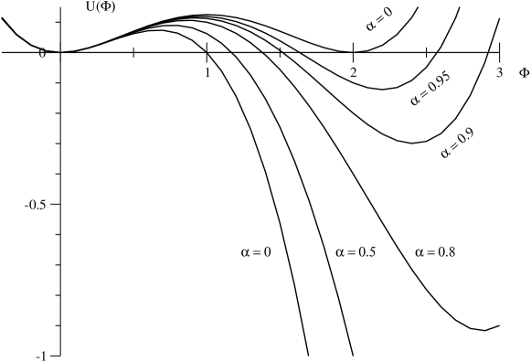
Figure 1: Potential $U(\Phi)$ in dimensionless form Eq. (3.4). The curves are labelled with the value of $\alpha$.

where the field potential $U(\varphi)$ is assumed to have two non-degenerate minima $\varphi=\varphi_{-}$ and $\varphi=\varphi_{+}>0$ (compare Fig. 1) and it will be given explicitly in the next section. For convenience we have fixed the value of $\varphi$ in the unstable vacuum as $\varphi_{-}=0$.

Any state built on the local minimum $\varphi_{-}$ is metastable. It can tunnel locally towards the $\varphi_{+}$ phase. The tunnelling rate per unit volume per unit time, $\gamma=\Gamma/VT$, is supposed to be dominated by the classical action $S_{cl}$ of a field configuration, the bounce $\varphi_{b}(x)$, which looks like a bubble of the $\varphi_{+}$-phase within the $\varphi_{-}$ phase. In particular it can be shown [28] that the bounce configuration $\varphi_{b}(x)$ which minimizes the action is spherically symmetric in four-dimensional Euclidean space. In the tree level approximation the decay rate is determined essentially by the tunnelling coefficient, $\gamma\propto\exp\{-S_{cl}[\varphi_{b}(x)]\}$.

The tree level tunnelling rate receives corrections in higher orders of the semiclassical approximation. In quantum field theory the fluctuations around the bounce contribute in the next-to-leading order approximation a pre-exponential factor to the decay rate. The rate per volume and time is known to take the form [5]

$$\gamma=\left(\frac{S_{cl}[\varphi]}{2\pi}\right)^{2}\left|{\cal D}\right|^{-1/2}\exp\left\{-S_{cl}[\varphi]-S_{ct}[\varphi]\right\}$$ (2.2)

to one-loop accuracy. The coefficient ${\cal D}$ here is defined as

$${\cal D}[\varphi]\equiv\frac{\det^{\prime}(-(\partial/\partial\tau)^{2}-\Delta+U^{\prime\prime}(\varphi))}{\det(-(\partial/\partial\tau)^{2}-\Delta+U^{\prime\prime}(0))}=\frac{\det^{\prime}({\cal M})}{\det({\cal M}^{(0)})}\;.$$ (2.3)

The prime in the determinant implies omitting of the four translation zero modes. With the second equation we have introduced the fluctuation operator in the background of the bounce

$${\cal M}=-(\partial/\partial\tau)^{2}-\Delta+U^{\prime\prime}(\varphi)$$ (2.4)

and its counterpart ${\cal M}^{(0)}$ in the unstable vacuum.

The counterterm action $S_{ct}$ is necessary in order to absorb the divergences of the one-loop effective action

$$S^{eff}_{1-loop}[\varphi]=\frac{1}{2}\ln|{\cal D}[\varphi]|.$$ (2.5)

In order to evaluate the one loop effective action we decompose fluctuations about the bounce $\varphi_{b}$ into $O(4)$ spherical harmonics, calculate the ratio of determinants $J_{l}$ of partial wave fluctuation operators and obtain $\ln{\cal D}$ as $\sum_{l}d_{l}\ln J_{l}$, where $d_{l}$ is the $O(4)$ degeneracy $d_{l}=(l+1)^{2}$ (see e.g. [29]). In calculating $\ln{\cal D}$ we exclude the divergent perturbative contributions of first and second order in the external field of the bounce $\varphi_{b}$. The regularized values of these contributions are then added analytically. All divergences of $\ln{\cal D}$ appear in the standard tadpole and fish diagrams. We will not specify $S_{ct}$ explicitly, we will equivalently omit the divergent parts of $\ln{\cal D}[\varphi]$ using the $\overline{MS}$ convention.

3 The Tree-Level Action

In this section we specify our model, discuss the bounce solution and properties of corresponding classical action. We parameterize the $\varphi^{4}$-potential with two minima as

$$U(\varphi)=\frac{1}{2}m^{2}\varphi^{2}-\eta\varphi^{3}+\frac{1}{8}\lambda\varphi^{4}\;,$$ (3.1)

and choose the same dimensionless variables as in Ref. [30, 10]: $x^{\mu}=X^{\mu}/m$ for $\mu=0,1,2,3$, and $\varphi=\frac{m^{2}}{2\eta}\Phi$. The classical action then takes the form

$$S_{cl}(\varphi)=\beta\tilde{S}_{cl}(\varphi)\;,$$ (3.2)

where rescaled classical action $\tilde{S}_{cl}(\varphi)$ is

$$\tilde{S}_{cl}(\varphi)=\int d^{4}X\left(\frac{1}{2}\left(\nabla\Phi\right)^{2}+U(\Phi)\right)\;,$$ (3.3)

with

$$U(\Phi)=\frac{1}{2}\Phi^{2}-\frac{1}{2}\Phi^{3}+\frac{\alpha}{8}\Phi^{4}\;,$$ (3.4)

and $\alpha$ and $\beta$

$$\beta=\frac{m^{2}}{4\eta^{2}},~{}\qquad\alpha=\lambda\beta.$$ (3.5)

being two dimensionless parameters . Parameter $\alpha$ varies from 0 to 1 and controls the strength of self–interaction and shape of the potential. For $\alpha=0$ the second minimum disappears, whereas in the limit $\alpha\to 1$ two minima become degenerate (see Fig. 1). Parameter $\beta$ controls size of the loop corrections. In order semiclassical approximation to be valid $\beta$ should not be too small (see Section 5 for details).

The bounce is non-trivial, $O(4)-$ symmetrical stationary point of $S_{cl}$, Eq. (3.3), obeying the Euler – Lagrange equation

$$\frac{d^{2}\Phi}{dR^{2}}+\frac{3}{R}\frac{d\Phi}{dR}-\Phi+\frac{3}{2}\Phi^{2}-\frac{\alpha}{2}\Phi^{3}=0\;,$$ (3.6)

and boundary conditions

$$\frac{d\Phi}{dR}|_{R=0}=0,\qquad\Phi_{R\to\infty}=\Phi_{-}\;.$$ (3.7)

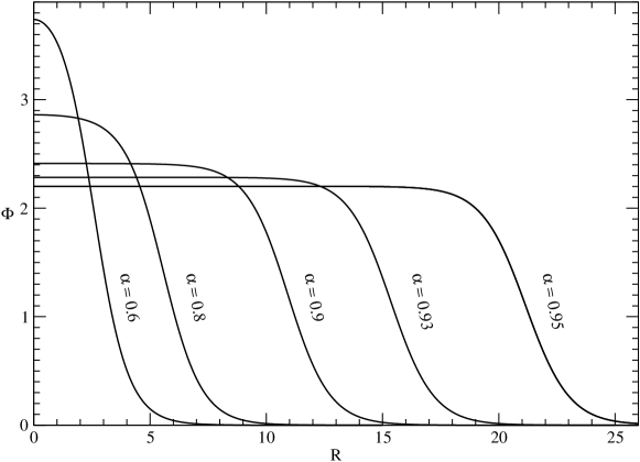
Figure 2: Bounce profiles for different $\alpha$.

Here $R=((X^{0})^{2}+|\vec{X}|^{2})^{1/2}$. The equation (3.6) at least for not very big $\alpha$ can be easily solved numerically, e.g., by the shooting method. We display some profiles $\Phi(R)$ in Fig. 2 for various values of the parameter $\alpha$ .

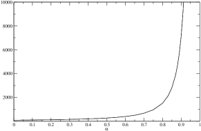
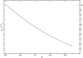
Figure 3: Classical action $\tilde{S}_{cl}$ versus $\alpha$ (left) and the ratio $\tilde{S}_{cl}/\tilde{S}^{tw}_{cl}$ for $\alpha>0.5$ (right).

The classical action $\tilde{S}_{cl}(\varphi)$ as a function of $\alpha$ is plotted in Fig. 3 (left). For small $\alpha$ classical action $S$ goes to a constant and $\tilde{S}_{cl}(\alpha=0)=90.857$. In the limit $\alpha\to 1$ the thin-wall case is realized (see Appendix A) and the classical action diverges as $(1-\alpha)^{-3}$. The ratio of the classical action computed numerically to the analytic thin-wall expression

$$\tilde{S}^{tw}_{cl}=\frac{\pi^{2}}{3(1-\alpha)^{3}}$$ (3.8)

is displayed in Fig. 3 (right). It tends to unity for $\alpha\to 1$, as it should. Note, that the radius of the bounce increases rapidly in this limit and numerical calculations become delicate. So, in the present article we restrict ourselves to the interval $\alpha\in[0,0.95]$.

4 Calculation of the Fluctuation Determinant

In this section we discuss a method of computing the ratio of functional determinants (2.3) which is based on earlier papers [7, 9, 10].

The explicit form of the operator in the nominator (2.3) is

$${\cal M}=-\Delta_{4}+m^{2}+V(r)\;.$$ (4.1)

Here $\Delta_{4}$ is the 4-dimensional Laplace operator, and we have introduced the potential $V$ as

$$V(r)=U^{\prime\prime}(\varphi)-m^{2}=-6\eta\varphi(r)+\frac{3}{2}\lambda\varphi^{2}(r)$$

$$=m^{2}\left[-3\Phi(R)+\frac{3}{2}\alpha\Phi^{2}(R)\right]\equiv m^{2}V(R)\;.$$ (4.2)

The “free” operator ${\cal M}^{(0)}$, corresponding to the metastable phase where $\varphi=0$ and where $m^{2}=U^{\prime\prime}(\varphi=0)$ takes the same form as (4.1), but with $V(r)=0$.

Due to the $O(4)$ spherical symmetry of the bounce the operators ${\cal M}$ and ${\cal M}^{(0)}$ can be separated with respect to $O(4)$ angular momentum. We introduce the partial wave operators

$${\bf M}_{l}(\nu)=-\frac{d^{2}}{dr^{2}}-\frac{3}{r}\frac{d}{dr}+\frac{l(l+2)}{r^{2}}+\nu^{2}+m^{2}+V(r)\;,$$ (4.3)

with an additional variable $\nu$ that will be used later on. In terms of these operators we can write

$${\cal D}[\varphi]\equiv{\prod_{l,n}}^{\prime}\left[\frac{\omega^{2}_{ln}}{{\omega^{{}2}_{ln{(0)}}}}\right]=\prod_{l=0}^{\infty}\left[\frac{\det^{\prime}{\bf M}_{l}(0)}{\det{\bf M}_{l}^{(0)}(0)}\right]^{d_{l}}\;,$$ (4.4)

where $d_{l}$ is the degeneracy of the $O(4)$ angular momentum, $d_{l}=(l+1)^{2}$. Prime denotes that for $l=1$ we have to remove the four translational zero modes.

The ratio of determinants of the radial operators

$$J_{l}(\nu)=\frac{\det{\bf M}_{l}(\nu)}{\det{\bf M}_{l}^{(\nu)}(0)}={\prod_{n}}\left[\frac{\omega^{2}_{ln}+\nu^{2}}{{\omega^{{}2}_{ln{(0)}}+\nu^{2}}}\right]$$ (4.5)

can be computed using the theorem on functional determinants as described in the next section. Note that $\omega^{2}_{ln}$ always denotes the eigenvalues of ${\bf M}_{l}(0)$, or more generally the eigenvalues of ${\cal M}$, the analogous definition holds for $\omega^{{}2}_{ln{(0)}}$.

4.1 Determinants of the Radial Operators

In order to find $J_{l}(\nu)$ (4.5) we make use of a known theorem [31, 6] whose statement is

$$\frac{\det{\bf M}_{l}(\nu)}{\det{\bf M}_{l}^{(0)}(\nu)}=\lim_{r\to\infty}\frac{\psi_{l}(\nu,r)}{\psi_{l}^{(0)}(\nu,r)}\;.$$ (4.6)

Here $\psi_{l}(\nu,r)$ and $\psi_{l}^{(0)}(\nu,r)$ are solutions to equations

$${\bf M}_{l}(\nu)\psi_{\nu,l}=0\;.\qquad{\bf M}_{l}^{(0)}(\nu)\psi_{\nu,l}^{(0)}=0\;,$$ (4.7)

and have same regular behavior at $r=0$. More exactly, the boundary conditions at $r=0$ must be chosen in such a way that the right-hand side of Eq. (4.6) tends to 1 at $\nu\rightarrow\infty$.

It is convenient to factorize the radial mode functions into the solution $\psi_{l}^{(0)}(\nu,r)$ for $V(r)=0$ and a factor $1+h_{l}(\nu,r)$ which takes into account the modification introduced by the potential. If $V(r)$ is of finite range the functions $\psi_{l}^{(0)}(\nu,r)$ and $\psi_{l}(\nu,r)$ have the same behavior near $r=0$ and as $r\to\infty$. Near $r=0$ they behave as $r^{l}$ and as $r\to\infty$ they behave as $\exp(-\kappa r)$ where $\kappa=\sqrt{\nu^{2}+m^{2}}$. Furthermore the requirement of analogous behavior near $r=0$ introduces the initial conditions $h(0)=h^{\prime}(0)=0$. The function $h(r)$ then simply starts from zero at $r=0$ and goes smoothly to a finite constant value $h_{l}(\nu,\infty)$ as $r\to\infty$. The solutions $\psi_{l}^{(0)}(\nu,r)$ are given in terms of modified Bessel functions as

$$\psi_{l}^{(0)}(\nu,r)=\frac{I_{l+1}(\kappa r)}{r}\;,$$ (4.8)

and we have

$$\psi_{l}(\nu,r)=\left[1+h_{l}(\nu,r)\right]\frac{I_{l+1}(\kappa r)}{r}\;.$$ (4.9)

Then by the theorem (4.6), the ratio of determinants (4.5) can be expressed as

$$J_{l}(\nu)=1+h_{l}(\nu,\infty)\;.$$ (4.10)

In terms of the $h$ function the first equation (4.7) reads

$$\left\{\frac{d^{2}}{dr^{2}}+\left[2\kappa\frac{I_{l+1}^{\prime}(\kappa r)}{I_{l+1}(\kappa r)}+\frac{1}{r}\right]\frac{d}{dr}\right\}h_{l}(\nu,r)=V(r)\left[1+h_{l}(\nu,r)\right]\;,$$ (4.11)

where $I_{l+1}^{\prime}(\kappa r)\equiv dI_{l+1}(\kappa r)/d(\kappa r)$.

In what follows it would be convenient to consider the perturbation expansion

$$h_{l}(\nu,r)=\sum_{k=1}^{\infty}h^{(k)}_{l}(\nu,r)$$ (4.12)

in powers of the potential $V(r)$. This assumes an analogous expansion for the ratios $J_{l}(\nu)$ in the sense that $J_{l}^{(k)}(\nu)=h_{l}^{(k)}(\nu,\infty)$. The $k$-order contribution $h_{l}^{(k)}$ obeys an equation

$$\left\{\frac{d^{2}}{dr^{2}}+\left[2\kappa\frac{I_{l+1}^{\prime}(\kappa r)}{I_{l+1}(\kappa r)}+\frac{1}{r}\right]\frac{d}{dr}\right\}h_{l}^{(k)}(\nu,r)=V(r)h_{l}^{(k-1)}(\nu,r)\;,$$ (4.13)

where we defined $h_{l}^{(0)}\equiv 1$. Since Eq. (4.13) is linear differential equation it holds also for linear combinations of $h_{l}^{(k)}$. It is convenient to introduce notation $h_{l}^{\overline{(k)}}=\sum_{q=k}^{\infty}h_{l}^{(q)}$. In this notation $h_{l}=h_{l}^{\overline{(1)}}$. A Green function that gives the solution to equation (4.13) in the form

$$h_{l}^{\overline{(k)}}(r)=-\int_{0}^{\infty}d{\tilde{r}}{\tilde{r}}G_{l}(r,{\tilde{r}})V({\tilde{r}})h_{l}^{\overline{(k-1)}}({\tilde{r}})$$ (4.14)

with the right boundary condition at $r=0$ reads

$$G_{l}(r,{\tilde{r}})=\frac{I_{l+1}(\kappa{\tilde{r}})}{I_{l+1}(\kappa r)}\left[I_{l+1}(\kappa r_{<})K_{l+1}(\kappa r_{>})-I_{l+1}(\kappa r)K_{l+1}(\kappa{\tilde{r}})\right]\;,$$ (4.15)

where $r_{<}=\min\{r,{\tilde{r}}\}$, $r_{>}=\max\{r,{\tilde{r}}\}$.

The first term on the right-hand side of Eq.(4.15) does not contribute to $h_{l}^{(k)}(\infty)$. The Green function (4.15) gives rise to connected graphs as well as disconnected ones. The latter are cancelled in $\ln(1+h_{l}(\infty))$ whose expansion in $k$-order connected graphs $J^{(k)}_{l~{}con}(\nu)$ reads

$$\ln J_{l}(\nu)=\ln(1+h_{l}(\nu,\infty))=\sum_{k=1}^{\infty}\frac{(-1)^{k+1}}{k}J^{(k)}_{l~{}con}(\nu)\;.$$ (4.16)

This formula is analogous to the expansion of the full functional determinant in terms of Feynman diagrams

$$\ln{\cal D}=\sum_{k=1}^{\infty}\frac{(-1)^{k+1}}{k}A^{(k)}\;,$$ (4.17)

where $A^{(k)}$ is the one-loop Feynman graph of order $k$ in the external potential $V(r)$.

Indeed, it is obvious from Eq.(4.14) that $h_{l}^{(k)}$ and, therefore, $J^{(k)}_{l~{}con}$ are of the order $V^{k}$. Since the expansion of $\ln{\cal D}$ in powers of $V$ is unique, we conclude that

$$A^{(k)}=\sum_{l=0}^{\infty}(l+1)^{2}J^{(k)}_{l~{}con}\;.$$ (4.18)

4.2 Calculation of ${\cal D}^{\overline{(3)}}$

Making use of a uniform asymptotic expansion of the modified Bessel functions in (4.15) one can check that that $J^{(k)}_{l~{}con}\sim 1/l^{2k-1}$ as $l\rightarrow\infty$. That results in the expected quadratic and logarithmic ultraviolet divergences in $\ln{\cal D}$ due to the contribution of $J^{(1)}_{l~{}con}$ and $J^{(2)}_{l~{}con}$. Our strategy is to compute analytically the first two terms in the sum Eq. (4.17) and to add numerically computed $\ln{\cal D}^{\overline{(3)}}$, which is the sum without first and second order diagrams $A^{(1)}$ and $A^{(2)}$. It reads explicitly

$$\ln{\cal D}^{\overline{(3)}}=\sum_{l=0}^{\infty}(l+1)^{2}\left(\ln J_{l}(\nu)\right)^{\overline{(3)}}\;,$$ (4.19)

where

$$\left(\ln J_{l}(\nu)\right)^{\overline{(3)}}=\ln\left(1+h_{l}(\infty)\right)-h_{l}^{(1)}(\infty)-\left[h_{l}^{(2)}(\infty)-\frac{1}{2}\left(h_{l}^{(1)}(\infty)\right)^{2}\right]\;.$$ (4.20)

The terms in square brackets here correspond to the fish diagram $J^{(2)}_{l~{}con}$. Since all contributions to $\ln{\cal D}^{\overline{(3)}}$ are ultraviolet finite, we need no regularization in computing them. The divergent contributions of the first and second order in $V$ will be considered in Sec. 4.3.

In order to avoid numerical subtraction that might be delicate we re-write the term (4.20) to be summed up on the right-hand side (4.19) in the form

$$\displaystyle\left(\ln J_{l}(\nu)\right)^{\overline{(3)}} = \left[\ln(1+h_{l}(\infty))-h_{l}(\infty)+\frac{1}{2}h_{l}(\infty)^{2}\right]$$ (4.21)

$$+~{}h_{l}^{\overline{(3)}}(\infty)-\frac{1}{2}h_{l}^{\overline{(2)}}(\infty)\left(h_{l}(\infty)+h_{l}^{(1)}(\infty)\right)\;.$$

Each of the three terms on the r.h.s. is now manifestly of order $V^{3}$. The subtraction done in the square bracket is exact enough when the logarithm is calculated with double precision. We have determined $h_{l}(r)$ as solutions of Eq.(4.11) and $h_{l}^{(1)}(r)$, $h_{l}^{\overline{(2)}}(r)$ and $h_{l}^{\overline{(3)}}(r)$ as those of Eq.(4.13) using Runge-Kutta-Nyström integration method [32]. Of course we cannot integrate the differential equations until $r=\infty$. In fact we have integrated it up to the maximal value for which we know the profile $\phi(r)$, and therefore $V(r)$. This value is such, that the classical field has well reached its vacuum expectation value, and therefore $V(r)$ has become zero. This is the condition under which we can impose the asymptotic boundary condition for the classical profile. For such values the functions $h^{(k)}_{l}(r)$ have already become constant; indeed for $V(r)=0$ they have the exact form $a+bK_{l+1}(\kappa r)/I_{l+1}(\kappa r)$ and the second part decreases exponentially for $r>>1/\kappa$. In praxi we used values of $R$ up to $R_{\max}=mr_{\max}\simeq 20-30$.

We have neglected till now the existence of the negative mode $\omega_{0}^{2}<0$ for $l=0$ and four zero modes $\omega_{1}^{2}=0$ with $l=1$. The former results in negative value of $J_{0}(\nu)=1+h_{0}(\nu,\infty)$ at $\nu=0$. According to Eq.(2.2) one has to replace $\omega_{0}^{2}$ by $|\omega_{0}^{2}|$. That implies taking the absolute value of $J_{0}(0)$ in Eq.(4.19); indeed $J_{0}(0)$ is found to be negative.

The translational zero modes manifest themselves by the vanishing of $\omega^{2}_{10}=0$, the lowest radial excitation in the $l=1$ channel with degeneracy $(l+1)^{2}=4$, and thereby by the vanishing of $J_{1}(\nu)$ at $\nu=0$, see Eq.(4.5). This represents a good check for both the classical solution and for the integration of the partial waves. The factor $\nu^{2}$ has to be removed according to the definition of $\det^{\prime}$. So in the $l=1$ contribution we have to replace $J_{1}(0)$ by

$$\lim_{\nu\to 0}\frac{J_{1}(\nu)}{\nu^{2}}=\frac{dJ_{1}(\nu)}{d\nu^{2}}=\frac{d}{d(\nu^{2})}h_{1}(\nu,\infty){\mid}_{\nu=0}\;.$$ (4.22)

Notice that replacement Eq. (4.22) introduces a dimension into the functional determinant. Thereby the units used for $\nu$ become the units of the transition rate. Here we have used the scale $m$ throughout, see Eqs. (5.1) and (5.2).

Our next step is performing summation over $l$ in Eq.(4.19). For small bounces ($\alpha\lesssim 0.8$) we have found good agreement with the expected behavior, namely

$$\left(\ln J_{l}(\nu)\right)^{\overline{(3)}}\propto\frac{1}{(l+1)^{5}}\;.$$ (4.23)

So, the summation has been done by cutting the sum at some value $l_{max}$ and adding the rest sum from $l_{max}+1$ to $\infty$ of terms fitted with

$$\ln J_{l}^{\overline{(3)}}\approx\frac{a}{(l+1)^{5}}+\frac{b}{(l+1)^{6}}+\frac{c}{(l+1)^{7}}\;.$$ (4.24)

The summation was stopped when increasing of $l_{max}$ by unity did not change the result within some given accuracy $\delta$. The required accuracy was decreased for higher $\alpha$. The problem is that the convergence becomes worse as we get closer to $\alpha=1$. This is related to the fact that the asymptotic behavior (4.23) sets in only when $l\gg mr_{\rm eff}$, where $r_{\rm eff}$ is the characteristic size of the bounce. It is of order $1/m$ at small values of $\alpha$ and can be estimated as $1/(1-\alpha)m$ near the thin-wall limit, $\alpha\rightarrow 1$. As the maximal value of the angular momentum that we have used is $l=25$, our computations cease to be reliable beyond $\alpha\simeq 0.95$. The value of $\delta$ was about $10^{-5}$ for small bounces, and of order of $10^{-3}$ for $\alpha>0.85$. As we will see below, for larger values of $\alpha$ the effective action is well approximated by the leading terms of a gradient expansion.

4.3 Perturbative contribution and renormalization

We have described in the previous subsection the computation of the finite part $\ln{\cal D}^{\overline{(3)}}$ which is the sum of all one-loop diagrams of the third order and higher,

$$\ln{\cal D}^{\overline{(3)}}=\sum_{k=3}^{\infty}\frac{(-1)^{k+1}}{k}A^{(k)}~{}~{}~{}.$$ (4.25)

We now have to discuss the leading divergent contributions $A^{(1)}$ and $A^{(2)}$. These are computed as ordinary Feynman graphs. Using dimensional regularization we have

$$A^{(1)}=\int\frac{d^{4-\epsilon}k}{(2\pi)^{4-\epsilon}}\frac{\tilde{V}(0)}{k^{2}+m^{2}}$$ (4.26)

where we have introduced the Fourier transform of the potential

$$\tilde{V}(k)=\int d^{4}xV(x)e^{-ikx}\;.$$ (4.27)

We obtain

$$A^{(1)}=-\frac{m^{2}}{16\pi^{2}}\left[\frac{2}{\epsilon}-\gamma_{E}+\ln 4\pi+\ln\frac{\mu^{2}}{m^{2}}+1\right]\int d^{4}xV(x)\;,$$ (4.28)

where $\mu$ is the usual dimensional regularization parameter. We choose it to be equal to $m$. Then using the $\overline{MS}$ scheme we just retain the last contribution in the bracket (see e.g. [33], p. 377). Thus, the finite part of $A^{(1)}$ is

$$A^{(1)}_{fin}=-\frac{1}{8}\int_{0}^{\infty}R^{3}dR~{}V(R)\;.$$ (4.29)

The second order terms takes the form

$$A^{(2)}=\int\frac{d^{4-\epsilon}q}{(2\pi)^{4-\epsilon}}\biggl{|}\tilde{V}(q)\biggr{|}^{2}\int\frac{d^{4-\epsilon}k}{(2\pi)^{4-\epsilon}}\frac{1}{(k^{2}+m^{2})[(k+q)^{2}+m^{2}]}\;.$$ (4.30)

We obtain

$$A^{(2)} = \frac{1}{16\pi^{2}}\left[\frac{2}{\epsilon}-\gamma_{E}+\ln 4\pi+\ln\frac{\mu^{2}}{m^{2}}\right]\int d^{4}x(V(x))^{2}$$

$$+\frac{1}{128\pi^{4}}\int q^{3}dq\biggl{|}\tilde{V}(q)\biggr{|}^{2}\left[2-\frac{\sqrt{q^{2}+4m^{2}}}{q}\ln\frac{\sqrt{q^{2}+4m^{2}}+q}{\sqrt{q^{2}+4m^{2}}-q}\right]\;.$$

Again the $\overline{MS}$ scheme corresponds to omitting the first term on the right hand side and for the finite part of $A^{(2)}$ we find

$$A^{(2)}_{fin}=\frac{1}{128\pi^{4}}\int_{0}^{\infty}Q^{3}dQ\biggl{|}\tilde{V}(Q)\biggr{|}^{2}\left[2-\sqrt{Q^{2}+4}~{}\ln\frac{\sqrt{Q^{2}+4}+Q}{\sqrt{Q^{2}+4}-Q}\right]\;,$$ (4.32)

with $Q=q/m$ being the dimensionless momenta. For the numerical evaluation of $A^{(2)}$ we have to compute the Fourier transform of the external potential which is known numerically, the remaining computation is straightforward.

5 Numerical results

To summarize we represented the false vacuum decay rate per unit time per unit volume as

$$\gamma=m^{4}\left(\frac{S_{cl}[\varphi]}{2\pi}\right)^{2}{\rm e}^{-S_{cl}[\varphi]-S^{eff}_{1-loop}[\varphi]}\;,$$ (5.1)

where

$$S^{eff}_{1-loop}[\varphi]=\frac{1}{2}\ln|m^{8}{\cal D}[\varphi]|=S^{eff}_{\rm 1-loop,p}+S^{eff}_{\rm 1-loop,n.p.}\;,$$ (5.2)

with perturbative

$$S^{eff}_{\rm 1-loop,p}=\frac{1}{2}(A^{(1)}_{fin}-\frac{1}{2}A^{(2)}_{fin})$$ (5.3)

and non perturbative

$$S^{eff}_{\rm 1-loop,n.p.}=\frac{1}{2}\sum_{k=3}^{\infty}\frac{(-1)^{k+1}}{k}A^{(k)}=\frac{1}{2}\ln|{\cal D}^{\overline{(3)}}|$$ (5.4)

contributions.

It is useful to introduce the quantity $G$,

$$G(\alpha,\beta)=S^{eff}_{\rm 1-loop}[\varphi]/S_{cl}[\varphi_{b}]\;,$$ (5.5)

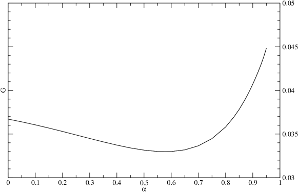
Figure 4: The ratio $G(\alpha,\beta)=S^{eff}_{1-loop}/S_{cl}$ for $\beta=1$.

which indicates how big quantum corrections are. Since classical action, Eq. (3.2), depends linearly on parameter $\beta$ we have $G(\alpha,\beta)=G(\alpha,1)/\beta$. Numerical calculation shows that that $G(\alpha,1)$ varies from 0.0367 to 0.0448 as we vary $\alpha$ from 0 to 0.95, with shallow minimum $G_{min}\approx 0.033$ at $\alpha$ about 0.6 (see Fig. 4). Fig. 4 suggests that $G(1,1)\approx 0.05$, which means that for sufficiently big values of $\beta$, namely $\beta>0.1$, the quantum corrections to the classical action are small (less then $50\%$) for all values of $\alpha$.

The corrections to the transition rate are given directly by a factor $\exp(-S^{eff}_{\rm 1-loop})$, so even if the classical transition rate is sizeable, as it happens for small $\beta$, the quantum corrections suppress the decay of the false vacuum by factors $\exp(-3.3)$ at $\alpha=0$ and $\exp(-291)$ at $\alpha=.9$.

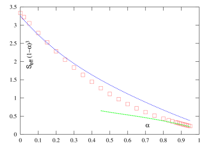
Figure 5: Our results for the effective action $S^{eff}_{\rm 1-loop}$ (squares) together with the perturbative part $S^{eff}_{\rm 1-loop,p}$ (dotted line) and the leading parts of the gradient expansion $S^{eff}_{{\rm grad},0+2}$ (dashed line, $\alpha=0.45-0.95$). All shown quantities are multiplied by the factor $(1-\alpha)^{3}$.

Note that the main contribution to the effective action for all $\alpha$ is coming from the $A^{(1)}_{fin}$, (comp. Tab. 1, Tab. 2). For small $\alpha$ perturbative contribution is almost $100\%$ of total one loop effective action, (comp. Fig. 5).

In the limit $\alpha\to 1$ the leading terms of the gradient expansion (Appendix B) gives dominant contribution to the one loop effective action. Already for $\alpha=0.8$ the sum of leading gradient terms

$$S^{eff}_{\rm grad,0+2}=S^{eff}_{{\rm grad},0}+S^{eff}_{{\rm grad},2}$$ (5.6)

approximates the $1-$loop effective action $S^{eff}_{\rm 1-loop}$ within 20$\%$. So the gradient expansion reproduces well the behavior of the one-loop effective action when $\alpha\to 1$, see Fig. 5. As the numerical procedure described in the main part of this paper becomes precarious for $\alpha\gtrsim 0.9$ this expansion complements the computation of the transition rate in this region.

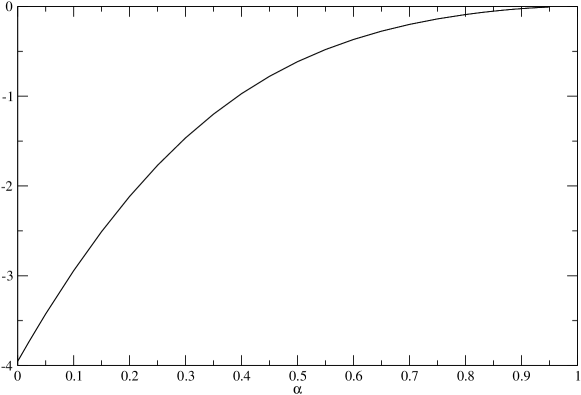
Figure 6: The negative mode energy as a function of $\alpha$

As it is well known there is exactly one negative mode in the spectrum of fluctuations about the bounce. Its energy is plotted vs $\alpha$ in Fig. 6.

In the present paper we used dimensional regularization and have chosen the parameter $\mu^{2}$, which can be understood as parameterizing a sequence of possible renormalization conditions, to be equal $m^{2}$. Choosing $\mu^{2}$ differently would result in the following corrections to $A^{(1)}_{fin}$ and $A^{(2)}_{fin}$

$$A^{(1)}_{fin}\to(1+\ln\frac{\mu^{2}}{m^{2}})A^{(1)}_{fin}$$

$$A^{(2)}_{fin}\to A^{(2)}_{fin}+a^{(2)}\ln\frac{\mu^{2}}{m^{2}}$$ (5.7)

where $a^{(2)}$ is the following integral

$$a^{(2)}=\frac{1}{8}\int_{0}^{\infty}R^{3}dR(V(R))^{2}$$ (5.8)

evaluated at the bounce solution. Numerical values for $A^{(1)}_{fin},A^{(2)}_{fin}$ and $a^{(2)}$ for different values of $\alpha$ are collected in Tab. 2. With the present choice of $\mu^{2}$ the perturbative terms represent the most important contributions to the effective action (see above), this means at the same time that a modification of the regularization and renormalization procedures can result in large changes in the one-loop effective action.

6 Discussion and Conclusion

In the present paper we applied previously developed technique for evaluations of functional determinants and calculated quantum corrections to the tunnelling transitions in 3+1 dimensional model of one self-interacting scalar field.

In the present toy model decay rate is vanishingly small. The sign of quantum corrections is such that it decreases false vacuum decay rate. The corrections can be thought as originating from the particles creation during the phase transitions. The created particles take energy from the tunnelling field and therefore decrease tunnelling probability. Analytical estimations show that particle creation is typically weak in the thin-wall approximation [25]. In the present paper it was found that the quantum corrections are even smaller away from the thin-wall case (compare Fig. 4), which assumes that particle creation for $\beta>0.1$ is weak for all values of the coupling constant $\alpha$. On the other hand for $\beta<0.1$ the quantum corrections dominate, which means that in this regime one should look for a bounce solution taking into account the full effective action in the one-loop approximation [26, 27].

Corrections to the false vacuum decay in a similar model in (3+1) dimensional theory in the thin wall approximation with the heat kernel expansion technique were calculated in [34], but it is not straightforward to compare our results since we use a different renormalization scheme and and a different parametrization of the potential. Powerful techniques for analytic calculations of the pre-factor using different approximations were developed in [23, 35, 36], but we cannot compare our results directly, since these calculations are within 3d theory.

The technique described here can be applied to tunnelling transitions in more realistic theories in 4 dimensions.

Appendix A. The thin-wall approximation

In the limit $\alpha\to 1$ so called thin-wall case is realized. This is when energy density difference $\epsilon$ between two vacuums

$$\epsilon=U(\Phi_{-})-U(\Phi_{+})\;,$$ (A.1)

is small (compare to the hight of the barrier). In this case potential Eq. (3.4) can be represented as

$$U(\Phi)=U_{0}(\Phi)+O(\epsilon)\;,$$ (A.2)

where symmetric part, $U_{0}$, in our case is

$$U_{0}(\Phi)=\frac{1}{8}\Phi^{2}(2-{\Phi})^{2}\;,$$ (A.3)

and

$$\epsilon=2(1-\alpha)\;,$$ (A.4)

In the thin-wall approximation the radius $\bar{R}$ of the bounce and the Euclidean action $S_{cl}$ are given analytically [4, 6] as

$$\bar{R}=\frac{3S_{1}}{\epsilon},\qquad\tilde{S}^{tw}_{cl}=\frac{27\pi^{2}S_{1}^{4}}{2\epsilon^{3}}\;,$$ (A.5)

where

$$S_{1}=2\int_{-\infty}^{\infty}dR~{}~{}U_{0}(\Phi_{k})\;,$$ (A.6)

is the action of the one-dimensional kink solution corresponding to degenerate potential $U_{0}$ with the equal minima. For our choice of the potential, Eq. (A.3), the kink solutions is

$$\Phi_{k}=\frac{2}{1+{\rm e}^{(R-\bar{R})}}\;.$$ (A.7)

One finds that $S_{1}=2/3$ and correspondingly

$$\bar{R}=\frac{1}{1-\alpha},\qquad\tilde{S}^{tw}_{cl}=\frac{\pi^{2}}{3(1-\alpha)^{3}}\;.$$ (A.8)

Appendix B. The leading terms of the gradient expansion

We want to derive an approximation to the effective action of a scalar field on the background of a bounce solution. The strategy is to expand first the effective action with respect to external vertices, and to expand in a second step the resulting Feynman amplitudes with respect to the external momenta. This approach is fairly standard, and has been used, e.g., in Ref. [24]. We note that we will retain all powers in the external vertices; such a summation was found to yield a very good approximation for the sphaleron determinant [11, 12], see Fig. 1 in the second entry of Ref. [12]. We have to compute the trace log or log det of a generalized Euclidean Klein-Gordon operator $\Delta_{4}+U^{\prime\prime}(\phi)$ where $\Delta_{4}$ is the four-dimensional Laplace operator. Formally

$$\left[\ln{\cal D}\right]=\ln\left[\frac{-\Delta_{4}+U^{\prime\prime}(\phi)}{-\Delta_{4}+U^{\prime\prime}(0)}\right]\;.$$ (B.1)

We introduce a potential $V(x)$ via

$$U^{\prime\prime}(\phi(x))=m^{2}+V(x)\;;\;\;\;U^{\prime\prime}(0)=m^{2}\;.$$ (B.2)

For the bounce the potential depends only on $r=|x|$ but we will not use this now. The logarithm can be expanded with respect to the potential $V(x)$. We write

$$\left[\ln{\cal D}\right] = \ln\left[\frac{-\Delta_{4}+m^{2}+V(x)}{-\Delta_{4}+m^{2}}\right]$$

$$= \ln\left[(-\Delta_{4}+m^{2})^{-1}(\Delta_{4}+m^{2}+V(x))\right]$$

$$= \ln\left[1+(-\Delta_{4}+m^{2})^{-1}V(x)\right]$$

$$= \sum_{N=1}^{\infty}\frac{(-1)^{N+1}}{N}\left[(-\Delta_{4}+m^{2})^{-1}V(x)\right]^{N}\;,$$

and the effective action is given by

$$S^{\rm eff}=\sum_{N=1}^{\infty}\frac{(-1)^{N+1}}{2N}{\rm tr}\left[(-\Delta_{4}+m^{2})^{-1}V(x)\right]^{N}\;.$$ (B.4)

We introduce the Fourier transform

$$\tilde{V}(q)=\int e^{-iq\cdot x}V(x)d^{4}x\;.$$ (B.5)

The individual terms in the expansion of the effective action have the form of Feynman diagrams with external sources $V(q_{j})$ with $j=1\dots k$. The momentum that has flown into the line $l$ is

$$Q_{l}=\sum_{j=1}^{l}q_{j}\;,$$ (B.6)

of course the total momentum must be zero,i.e., $Q_{N}=0$. With these notations we can write the $N$th term in the effective action, omitting the factor $(-1)^{N+1}/2N$ as

$$A_{N}=\int\frac{d^{4}p}{(2\pi)^{4}}\prod_{j=1}^{N}\left[\int\frac{d^{4}q_{j}}{(2\pi)^{4}}\tilde{V}(q_{j})\right]\prod_{l=1}^{N}\left[\frac{1}{(p+Q_{l})^{2}+m^{2}}\right](2\pi)^{4}\delta(Q_{N})\;.$$ (B.7)

The four-momentum delta function arises from taking the trace. We obtain a gradient expansion by expanding the denominators $(p+Q_{l})^{2}+m^{2}$ with respect to the momenta $Q_{l}$. The leading term is of course

$$A_{N,0} = \int\frac{d^{4}p}{(2\pi)^{4}}\left[\frac{1}{p^{2}+m^{2}}\right]^{N}\prod_{j=1}^{N}\left[\int\frac{d^{4}q_{j}}{(2\pi)^{4}}\tilde{V}(q_{j})\right](2\pi)^{4}\delta(Q_{N})$$ (B.8)

$$= \int\frac{d^{4}p}{(2\pi)^{4}}\left[\frac{1}{p^{2}+m^{2}}\right]^{N}\int d^{4}x\left[V(x)\right]^{N}\;.$$

The zero-gradient contribution to the effective action is obtained by resuming this series; one finds

$$S^{\rm eff}_{{\rm grad},0}=\frac{1}{2}\int d^{4}x\int\frac{d^{4}p}{(2\pi)^{4}}\ln\left\{\frac{p^{2}+U^{\prime\prime}(\phi)}{p^{2}+U^{\prime\prime}(0)}\right\}\equiv\frac{1}{2}\int d^{4}xK^{(4)}\;.$$ (B.9)

Of course this integral has to be regularized, e.g., via dimensional regularization. The divergences come form the terms with $N=1$ and $N=2$, which are standard divergent one loop integrals.

We find

$$K^{(D)} = \frac{2\pi^{D/2}}{\Gamma\left(\frac{D}{2}\right)}\int\frac{dp\,p^{D-1}}{(2\pi)^{D}}\ln\left[\frac{p^{2}+U^{\prime\prime}(\phi)}{p^{2}+U^{\prime\prime}(0)}\right]$$

$$= \frac{2}{\Gamma\left(\frac{D}{2}\right)(4\pi)^{D/2}}\left\{\frac{1}{D}p^{D}\ln\left[\frac{p^{2}+U^{\prime\prime}(\phi)}{p^{2}+U^{\prime\prime}(0)}\right]\biggl{|}_{p=0}^{\infty}\right.$$

$$\left.\hskip 28.45274pt-\frac{2}{D}\int dp\,p^{D+1}\left[\frac{1}{p^{2}+U^{\prime\prime}(\phi)}-\frac{1}{p^{2}+U^{\prime\prime}(0)}\right]\right\}\;.$$

The first term in the parenthesis vanishes for $0<D<2$ and is defined to vanish in general by analytic continuation. The second term can be rewritten as

$$\frac{-2}{D\Gamma\left(\frac{D}{2}\right)(4\pi)^{D/2}}\left\{[U^{\prime\prime}(\phi)]^{D/2}-[U^{\prime\prime}(0)]^{D/2}\right\}\int_{0}^{\infty}dx\frac{x^{D+1}}{x^{2}+1}$$

$$=\frac{-2}{D\Gamma\left(\frac{D}{2}\right)(4\pi)^{D/2}}\frac{\Gamma(D/2+1)\Gamma(-D/2)}{2\Gamma(1)}\left\{[U^{\prime\prime}(\phi)]^{D/2}-[U^{\prime\prime}(0)]^{D/2}\right\}$$

$$=-\frac{\Gamma(-D/2)}{(4\pi)^{D/2}}\left\{[U^{\prime\prime}(\phi)]^{D/2}-[U^{\prime\prime}(0)]^{D/2}\right\}\;.$$

Now set $D=4-\epsilon$ and use

$$\Gamma\left(-\frac{D}{2}\right) = \frac{1}{(-2+\epsilon/2)(-1+\epsilon/2)}\Gamma\left(\frac{\epsilon}{2}\right)$$

$$= \frac{1}{2}\left\{\frac{2}{\epsilon}-\gamma_{E}+\frac{3}{2}\right\}$$

to obtain

$$K^{(4-\epsilon)} = \frac{-1}{32\pi^{2}}\left[\frac{2}{\epsilon}-\gamma_{E}+\ln 4\pi+\frac{3}{2}\right]$$

$$\times\left\{(m^{2}+V(r))^{2}\left[1-\frac{\epsilon}{2}\ln\frac{m^{2}+V(r)}{\mu^{2}})\right]-m^{4}\left[1-\frac{\epsilon}{2}\ln\frac{m^{2}}{\mu^{2}}\right]\right\}\;.$$

Using $\overline{MS}$ subtraction we get

$$K^{(4)} = \frac{-1}{32\pi^{2}}\left\{\frac{3}{2}\left[2m^{2}V(r)+V^{2}(r)\right]\right.$$

$$\left.-\left(m^{2}+V(r)\right)^{2}\ln\frac{m^{2}+V(r)}{\mu^{2}}+m^{4}\ln\frac{m^{2}}{\mu^{2}}\right\}\;.$$

Integrating over 4d Euclidean space we finally obtain

$$S^{eff}_{{\rm grad},0} = \frac{1}{32}\int^{\infty}_{0}R^{3}dR\left[\left(1+V(R)\right)^{2}\ln\frac{1+V(R)}{\tilde{\mu}^{2}}\right.$$ (B.11)

$$- \left.\frac{3}{2}\left(2V(R)+V^{2}(R)\right)+\ln\tilde{\mu}^{2}\right]\;,$$

with $\tilde{\mu}=\mu/m$.

Let us now consider the one- and two-gradient contributions. We expand the denominators up to second order in the gradients, i.e., in the momenta $Q_{j}$. We obtain

$$\Pi_{N} \equiv \prod_{l=1}^{N}\left[\frac{1}{(p+Q_{l})^{2}+m^{2}}\right]=\frac{1}{(p^{2}+m^{2})^{N}}-\frac{1}{(p^{2}+m^{2})^{N+1}}\sum_{j=1}^{N}2p\cdot Q_{j}$$ (B.12)

$$-\frac{1}{(p^{2}+m^{2})^{N+1}}\sum_{j=1}^{N}Q_{j}^{2}+\frac{1}{(p^{2}+m^{2})^{N+2}}\sum_{j=1}^{N-1}\sum_{k=j+1}^{N}4(p\cdot Q_{j})(p\cdot Q_{k})$$

$$+\frac{1}{(p^{2}+m^{2})^{N+2}}\sum_{j=1}^{N}4(p\cdot Q_{j})^{2}+O(Q^{3})pkt$$

Under $O(4)-$symmetric integration $4p_{\mu}p_{\nu}\simeq p^{2}\delta_{\mu\nu}$, and $p_{\mu}\simeq 0$. So the one-gradient term vanishes and the complete two-gradient contribution becomes

$$\Pi_{N,2} = \frac{1}{(p^{2}+m^{2})^{N+2}}\left[-(p^{2}+m^{2})\sum_{j}Q_{j}^{2}+4p_{\mu}p_{\nu}\sum_{k>j}Q_{j\mu}Q_{k\nu}+4p_{\mu}p_{\nu}\sum_{j}Q_{j\mu}Q_{j\nu}\right]$$ (B.13)

$$\simeq \frac{1}{(p^{2}+m^{2})^{N+2}}\left[p^{2}\sum_{k>j}Q_{j}\cdot Q_{k}-m^{2}\sum_{j}Q_{j}^{2}\right]\;.$$

We now have to rewrite this in terms of the momenta $q_{j}$ that represent the gradients on the functions $V(q_{j})$. After having used the fact that $\Pi_{2}$ appears under the integral over $d^{4}p$ we will now use the fact that it appears under the product of integrals $\int d^{4}q_{j}V(q_{j})$ which implies permutation symmetry in the indices $j$. So if we expand the products $Q_{j}\cdot Q_{k}$ and $Q_{j}^{2}$ we will encounter just two kinds of terms: products $q_{l}\cdot q_{m}$ with $l\neq m$ and squares $q_{l}^{2}$, which may be replaced by $q_{1}\cdot q_{2}$ and by $q_{1}^{2}$, respectively. We have to do some combinatorics in order to find

$$\sum_{j}Q_{j}^{2} \simeq \frac{(N-1)N(N+1)}{3}q_{1}\cdot q_{2}+\frac{N(N+1)}{2}q_{1}^{2}$$ (B.14)

$$\sum_{k>j}Q_{j}\cdot Q_{k} \simeq \frac{(N-1)N(N+1)(3N-2)}{24}q_{1}\cdot q_{2}$$ (B.15)

$$+\frac{(N-1)N(N+1)}{6}q_{1}^{2}\;.$$

Now we may use momentum conservation to rewrite

$$q_{1}^{2}=-q_{1}\cdot(q_{2}+\dots+q_{N})\simeq-(N-1)q_{1}\cdot q_{2}$$ (B.16)

so that

$$\sum_{j}Q_{j}^{2} \simeq -\frac{(N-1)N(N+1)}{6}q_{1}\cdot q_{2}$$ (B.17)

$$\sum_{k>j}Q_{j}\cdot Q_{k} \simeq -\frac{(N-2)(N-1)N(N+1)}{24}q_{1}\cdot q_{2}$$ (B.18)

and

$$\Pi_{N,2}\simeq\frac{1}{(p^{2}+m^{2})^{N+2}}\frac{(N-1)N(N+1)}{24}q_{1}\cdot q_{2}\left[-(N-2)p^{2}+4m^{2}\right]\;.$$ (B.19)

The momentum integrals are

$$\int\frac{d^{4}p}{(2\pi)^{4}}\frac{p^{2}}{(p^{2}+m^{2})^{N+2}} = \frac{1}{16\pi^{2}}m^{2-2N}\frac{2}{(N-1)N(N+1)}$$ (B.20)

$$\int\frac{d^{4}p}{(2\pi)^{4}}\frac{m^{2}}{(p^{2}+m^{2})^{N+2}} = \frac{1}{16\pi^{2}}m^{2-2N}\frac{1}{N(N+1)}$$ (B.21)

and, therefore,

$$\int\frac{d^{4}p}{(2\pi)^{4}}\Pi_{N,2}=q_{1}\cdot q_{2}\frac{1}{16\pi^{2}}m^{2-2N}\frac{N}{12}\;.$$ (B.22)

The momenta are converted into gradients; so we finally obtain as the expansion terms of the two-gradient part of the effective action

$$A_{N,2}=-\frac{1}{16\pi^{2}}\int d^{4}x\left[\frac{V(x)}{m^{2}}\right]^{N-2}\frac{N}{12m^{2}}\left(\nabla V(x)\right)^{2}\;.$$ (B.23)

The term $A_{1,2}$ is zero. The sum over all terms yields

$$S^{\rm eff}_{grad,2}=\frac{1}{32\pi^{2}}\int d^{4}x\frac{1}{m^{2}+V(x)}\frac{1}{12}\left(\nabla V(x)\right)^{2}\;,$$ (B.24)

or finally in dimensionless variables

$$S^{\rm eff}_{grad,2}=\frac{1}{192}\int_{0}^{\infty}R^{3}dR\frac{1}{1+V(R)}\left(V^{\prime}(R)\right)^{2}\;.$$ (B.25)

An alternative derivation starts with a technical step that frees us from the denominator $1/N$. We take the derivative of the effective action with respect to $m^{2}$, a step that we can revert later on. We then obtain, using the cyclic property of the trace,

$${\cal G} \equiv \frac{dS^{\rm eff}}{dm^{2}}$$

$$= \sum_{N=0}^{\infty}\frac{(-1)^{N}}{2}{\rm tr}\left\{\left[(-\Delta_{4}+m^{2})^{-1}V(x)\right]^{N}(-\Delta_{4}+m^{2})^{-1}\right\}$$

$$= \frac{1}{2}\sum_{N=0}^{\infty}B_{N}\;.$$

We note that we have included the $N=0$ term, which can be removed later on if necessary. So we have arrived at the trace of the exact Green function in the external field. The terms $B_{N}$ have the form

$$B_{N} = (-1)^{N}\int\frac{d^{4}p}{(2\pi)^{4}}\prod_{j=1}^{N}\left[\int\frac{d^{4}q_{j}}{(2\pi)^{4}}\right]\frac{1}{p^{2}+m^{2}}\tilde{V}(q_{1})\frac{1}{(p+Q_{1})^{2}+m^{2}}$$

$$\times\tilde{V}(q_{2})\frac{1}{(p+Q_{2})^{2}+m^{2}}\tilde{V}(q_{3})\dots$$

$$\times\tilde{V}(q_{N})\frac{1}{(p+Q_{N})^{2}+m^{2}}(2\pi)^{4}\delta(Q_{N})\;.$$

Assume we have expanded the fraction $1/[(p+Q_{k})^{2}+m^{2}]$ to first order in $2p\cdot Q_{k}+Q_{k}^{2}$, yielding a factor

$$\frac{1}{p^{2}+m^{2}}\left[-2p\cdot Q_{k}-Q_{k}^{2}\right]\frac{1}{p^{2}+m^{2}}$$ (B.28)

at the $k^{\rm th}$ place in the product of propagators and vertices, in other words we have obtained an insertion of $-2p\cdot Q_{k}-Q_{k}^{2}$. Consider the part of the product to the right of this insertion. We rewrite it as

$$\prod_{j=k+1}^{N} \left[\int\frac{d^{4}q_{j}}{(2\pi)^{4}}\right]\left[-2p\cdot Q_{k}-Q_{k}^{2}\right]\frac{1}{p^{2}+m^{2}}$$

$$\times \prod_{j=k+1}^{N} \left[\int d^{4}x_{j}V(x_{j})\frac{e^{-iq_{j}\cdot x_{j}}}{p^{2}+m^{2}}\right](2\pi)^{4}\delta(Q_{k}+q_{k+1}+\dots+q_{N})\;.$$ (B.29)

We furthermore rewrite the delta function as

$$(2\pi)^{4}\delta(Q_{k}+q_{k+1}+\dots+q_{N})=\int d^{4}xe^{i(Q_{k}+q_{k+1}+\dots+q_{N})\cdot x}\;.$$ (B.30)

Inserting this in (B.29) we can carry out the integrations over the $q_{j}$ and the $x_{j}$ to obtain

$$\int d^{4}xe^{iQ_{k}\cdot x}\left[-2p\cdot Q_{k}-Q_{k}^{2}\right]\frac{1}{p^{2}+m^{2}}\prod_{j=k+1}^{N}\left[V(x)\frac{1}{p^{2}+m^{2}}\right]\;.$$ (B.31)

Now the $Q_{k,\mu}$ in $2p\cdot Q_{k}+Q_{k}^{2}$ can be written as $-i\partial/\partial x_{\mu}=-i\partial_{\mu}$ on the exponential. Integrating by parts they can be written as $i\partial_{\mu}$ acting on the product to their right. So the whole string to the right of the insertion can be written as

$$\int d^{4}xe^{iQ_{k}\cdot x}\left[-2ip\cdot\partial+\partial^{2}\right]\frac{1}{p^{2}+m^{2}}\prod_{j=k+1}^{N}\left[V(x)\frac{1}{p^{2}+m^{2}}\right]\;.$$ (B.32)

We now consider the sum over $N$; we split $N=k+l$ and $(-1)^{N}=(-1)^{k}(-1)^{l}$. The sum over $l$ is independent of $k$ and runs from $0$ to $\infty$ and, putting in the factor $(-1)^{l}$ we obtain

$$\int d^{4}xe^{iQ_{k}\cdot x}\left[-2ip\cdot\partial+\partial^{2}\right]\frac{1}{p^{2}+m^{2}}\sum_{l=0}^{\infty}\prod_{j=1}^{l}\left[-V(x)\frac{1}{p^{2}+m^{2}}\right]$$ (B.33)

$$= \int d^{4}xe^{iQ_{k}\cdot x}\left[-2ip\cdot\partial+\partial^{2}\right]\frac{1}{p^{2}+m^{2}+V(x)}\;.$$

Note that the sum starts with $l=0$, which corresponds to the case $k=N$; in this case the product over $j$ reduces to $1$. Now we do the analogous operations on the part to the left of the insertion, using in the exponent $Q_{k}=q_{1}+\dots+q_{k}$; we now can carry out the summation over k and we find finally for the case that we have taken into account the first order expansion of one of the denominators $(p+Q_{k})^{2}+m^{2}$

$$\int d^{4}x\frac{1}{p^{2}+m^{2}+V(x)}\left[-2ip\cdot\partial+\partial^{2}\right]\frac{1}{p^{2}+m^{2}+V(x)}\;.$$ (B.34)

Obviously part $-i2p\cdot\partial$ vanishes upon symmetric integration over $p$. It also can be written as a boundary term for the $x$ integration. If we want to obtain the second order gradient term we have to take into account the $Q_{k}^{2}$ term of the first order expansion, i.e.

$$\int d^{4}x\frac{1}{p^{2}+m^{2}+V(x)}\partial^{2}\frac{1}{p^{2}+m^{2}+V(x)}\;,$$ (B.35)

the terms $-2ip\cdot\partial$ arising if two denominators are expanded to first order, yielding

$$\int d^{4}x\frac{1}{p^{2}+m^{2}+V(x)}(-2ip\cdot\partial)\frac{1}{p^{2}+m^{2}+V(x)}(-2ip\cdot\partial)\frac{1}{p^{2}+m^{2}+V(x)}\;.$$ (B.36)

Here is included the term arising from expanding one propagator to second order. Indeed this yields

$$\frac{1}{p^{2}+m^{2}}\left[-2p\cdot Q_{k}-Q_{k}^{2}\right]\frac{1}{p^{2}+m^{2}}\left[-2p\cdot Q_{k}-Q_{k}^{2}\right]\frac{1}{p^{2}+m^{2}}\;,$$ (B.37)

a term that is needed for obtaining the complete propagator $1/(p^{2}+m^{2}+V(x))$ between the two insertions. We now have the two-gradient term

$${\cal G}^{(2)} = \frac{1}{2}\int\frac{d^{4}p}{(2\pi)^{4}}\int d^{4}x\left\{\frac{1}{p^{2}+m^{2}+V(x)}\partial^{2}\frac{1}{p^{2}+m^{2}+V(x)}\right.$$

$$\left.+\frac{1}{p^{2}+m^{2}+V(x)}(-2ip\cdot\partial)\frac{1}{p^{2}+m^{2}+V(x)}(-2ip\cdot\partial)\frac{1}{p^{2}+m^{2}+V(x)}\right\}\;.$$

The first term can be written, after one integration by parts as

$$\frac{1}{2}\int\frac{d^{4}p}{(2\pi)^{4}}\int d^{4}x\frac{-1}{(p^{2}+m^{2}+V(x))^{4}}\left[\partial V(x)\right]^{2}\;.$$ (B.39)

In the second term we remark that the derivatives in the first insertion act on the complete part to the right of it. Therefore an integration by parts lets it act onto the part to the left of it. Using symmetric integration over $p$ the second part yields

$$\frac{1}{2}\int\frac{d^{4}p}{(2\pi)^{4}}\int d^{4}x\frac{p^{2}}{(p^{2}+m^{2}+V(x))^{5}}\left[\partial V(x)\right]^{2}\;.$$ (B.40)

Now we integrate with respect to $m^{2}$ to obtain the two-gradient contribution to the one-loop effective action

$$S^{\rm eff}_{{\rm grad},2} = \frac{1}{2}\int\frac{d^{4}p}{(2\pi)^{4}}\int d^{4}x\left[\frac{1}{3}\frac{1}{(p^{2}+m^{2}+V(x))^{3}}-\frac{1}{4}\frac{p^{2}}{(p^{2}+m^{2}+V(x))^{3}}\right]\left[\partial V(x)\right]^{2}$$ (B.41)

$$= \frac{1}{32\pi^{2}}\int d^{4}x\frac{1}{m^{2}+V(x)}\frac{1}{12}\left[\partial V(x)\right]^{2}\;,$$

which coincides with the previous result Eq. (B.24).

The terms of the gradient expansion can be evaluated in a straightforward way. We note, however, that the term $m^{2}+V(x)$ vanishes, depending on value of $\alpha$, at one or two points, and that therefore the expressions are ill-defined a priori. This is a reflection of the fact that the effective action has an imaginary part, due to the negative mode. An expansion of the effective action has to reflect this feature. With an $m^{2}-i\epsilon$ prescription this becomes apparent. When computing these terms we have used the principal value prescription for $S^{\rm eff}_{{\rm grad},2}$ and taken the absolute value in the logarithm appearing in $S^{eff}_{{\rm grad},0}$.

$\alpha$	$S^{eff}_{\rm 1-loop,p}$	$S^{eff}_{\rm 1-loop,n.p.}$	$S^{eff}_{1-loop}$	$\tilde{S}_{cl}$
0.00	3.253E+00	8.216E-02	3.335E+00	9.086E+01
0.02	3.337E+00	8.498E-02	3.422E+00	9.355E+01
0.05	3.478E+00	8.422E-02	3.562E+00	9.787E+01
0.10	3.752E+00	6.737E-02	3.819E+00	1.059E+02
0.15	4.089E+00	2.654E-02	4.115E+00	1.153E+02
0.20	4.504E+00	-4.501E-02	4.459E+00	1.263E+02
0.25	5.021E+00	-1.564E-01	4.865E+00	1.394E+02
0.30	5.672E+00	-3.201E-01	5.351E+00	1.552E+02
0.35	6.499E+00	-5.539E-01	5.946E+00	1.744E+02
0.40	7.571E+00	-8.836E-01	6.687E+00	1.983E+02
0.45	8.984E+00	-1.348E+00	7.637E+00	2.286E+02
0.50	1.089E+01	-2.006E+00	8.889E+00	2.681E+02
0.55	1.356E+01	-2.958E+00	1.060E+01	3.211E+02
0.60	1.741E+01	-4.371E+00	1.303E+01	3.951E+02
0.65	2.326E+01	-6.560E+00	1.670E+01	5.033E+02
0.70	3.277E+01	-1.015E+01	2.261E+01	6.720E+02
0.75	4.966E+01	-1.659E+01	3.306E+01	9.589E+02
0.80	8.382E+01	-2.969E+01	5.413E+01	1.512E+03
0.83	1.240E+02	-4.512E+01	7.887E+01	2.136E+03
0.85	1.686E+02	-6.233E+01	1.062E+02	2.809E+03
0.87	2.409E+02	-9.038E+01	1.506E+02	3.874E+03
0.88	2.950E+02	-1.114E+02	1.836E+02	4.655E+03
0.89	3.684E+02	-1.401E+02	2.283E+02	5.699E+03
0.90	4.711E+02	-1.803E+02	2.907E+02	7.140E+03
0.91	6.199E+02	-2.390E+02	3.809E+02	9.198E+03
0.92	8.455E+02	-3.284E+02	5.171E+02	1.227E+04
0.93	1.207E+03	-4.724E+02	7.347E+02	1.711E+04
0.94	1.829E+03	-7.209E+02	1.109E+03	2.531E+04
0.95	3.008E+03	-1.188E+03	1.820E+03	4.061E+04

Tab. 1. Numerical results for classical action and one loop effective action.

References

- [1] J. S. Langer, Ann.Phys. (N.Y.) 41 (1967) 108.
- [2] J. S. Langer, Ann.Phys. (N.Y.) 54 (1969) 258.
- [3] M. B. Voloshin, I. Y. Kobzarev and L. B. Okun, Sov. J. Nucl. Phys. 20 (1975) 644.
- [4] S. Coleman, Phys. Rev. D15 (1977) 2929.
- [5] C. G. Callan and S. R. Coleman, Phys. Rev. D 16 (1977) 1762.
- [6] S. Coleman, ’The Uses of Instantons’ in ”The Whys of Subnuclear Physics”, A. Zichichi ed., Plenum Press, New York 1979.
- [7] V. G. Kiselev and K. G. Selivanov, Sov. Phys. JTEP Lett. 39 (1984) 85.
- [8] V. G. Kiselev and K. G. Selivanov, Sov. J. Nucl. Phys. 43 (1986) 153.
- [9] K. G. Selivanov, Sov. Phys. JETP 67 (1988) 1548.
- [10] J. Baacke and V. G. Kiselev, Phys. Rev. D 48(1993) 5648, [arXiv: hep-ph/9308273].
- [11] L. Carson, X. Li, L. D. McLerran and R. T. Wang, Phys. Rev. D 42 (1990) 2127.
-
[12]
J. Baacke and S. Junker,
Phys. Rev. D 49 (1994) 2055,
[arXiv:hep-ph/9308310];
Phys. Rev. D 50 (1994) 4227, [arXiv:hep-th/9402078]. - [13] J. Baacke, Phys. Rev. D 52 (1995) 6760, [arXiv:hep-ph/9503350].
- [14] J. Baacke, Acta Phys. Pol. B22 (1991) 127 and references therein.
- [15] J. Baacke, Z. Phys. C53 (1992) 402.
- [16] J. Baacke and T. Daiber, Phys. Rev. D 51 (1995) 795, [arXiv:hep-th/9408010].
- [17] D. Diakonov, M. V. Polyakov, P. Sieber, J. Schaldach and K. Goeke, Phys. Rev. D 53 (1996) 3366, [arXiv:hep-ph/9502245].
- [18] N. Graham, R. L. Jaffe, V. Khemani, M. Quandt, M. Scandurra and H. Weigel, arXiv: hep-th/0207120.
- [19] M. Bordag, Phys. Rev. D 67 (2003) 065001, [arXiv:hep-th/0211080].
- [20] M. Hellmund, J. Kripfganz and M. G. Schmidt, Phys. Rev. D 50 (1994) 7650, [arXiv:hep-ph/9307284].
- [21] D. Fliegner, M. G. Schmidt and C. Schubert, Z. Phys. C 64 (1994) 111, [arXiv:hep-ph/9401221].
- [22] D. Fliegner, P. Haberl, M. G. Schmidt and C. Schubert, Annals Phys. 264 (1998) 51, [arXiv:hep-th/9707189].
- [23] G. Munster and S. Rotsch, Eur. Phys. J. C 12 (2000) 161, [arXiv:cond-mat/9908246].
- [24] J. Caro and L. L. Salcedo, Phys. Lett. B 309 (1993) 359.
- [25] V. A. Rubakov, Nucl. Phys. B 245 (1984) 481.
- [26] A. Surig, Phys. Rev. D 57 (1998) 5049, [arXiv:hep-ph/9706259].
- [27] D. Levkov, C. Rebbi and V. A. Rubakov, Phys. Rev. D 66 (2002) 083516, [arXiv:gr-qc/0206028].
- [28] S. Coleman, V. Glaser and A. Martin, Commun. Math. Phys. 58 (1978) 211.
- [29] P. Candelas and S. Weinberg, Nucl. Phys. B 237 (1984) 397.
- [30] M. Dine, R. G. Leigh, P. Huet, A. Linde, D. Linde, Phys.Rev. D46 (1992) 550; Phys. Lett. B283 (1992) 319.
- [31] R. F. Dashen, B. Hasslacher, and A. Neveu, Phys.Rev. D10 (1974) 4114; I. M. Gel’fand and A. M. Yaglom, J. Math. Phys. 1 (1960) 48; R. H. Cameron and W. T. Martin, Bull. Am. Math. Soc. 51 (1945) 73; J. H. van Vleck, Proc. Nat. Acad. Sci. 14 (1928) 178.
- [32] See e.g.: R. Zurmühl, Praktische Mathematik für Ingenieure und Physiker, Springer, 1984.
- [33] M. E. Peskin, D. V. Schroeder, Introduction to quantum field theory, Perseus Books, 1995.
- [34] R. V. Konoplich and S. G. Rubin, Sov. J. Nucl. Phys. 42 (1985) 810.
- [35] A. Strumia, N. Tetradis and C. Wetterich, Phys. Lett. B 467 (1999) 279, [arXiv:hep-ph/9808263].
- [36] G. Munster, A. Strumia and N. Tetradis, Phys. Lett. A 271 (2000) 80, [arXiv: cond-mat/0002278].