TUW–03–18

The Classical Solutions of the Dimensionally Reduced Gravitational Chern-Simons Theory

D. Grumiller, W. Kummer

Institut für Theoretische Physik, Technische Universität Wien
Wiedner Hauptstr. 8–10, A-1040 Wien, Austria

The Kaluza-Klein reduction of the 3d gravitational Chern-Simons term to a 2d theory is equivalent to a Poisson-sigma model with fourdimensional target space and degenerate Poisson tensor of rank 2. Thus two constants of motion (Casimir functions) exist, namely charge and energy. The application of well-known methods developed in the framework of first order gravity allows to construct all classical solutions straightforwardly and to discuss their global structure. For a certain fine tuning of the values of the constants of motion the solutions of hep-th/0305117 are reproduced. Possible generalizations are pointed out.

1 Introduction

As shown by the authors of ref. [1] the gravitational Chern-Simons term can be reduced by a Kaluza-Klein like ansatz (3.28), decomposing the 3d metric into a 2d metric $g_{\mu\nu}$, a $U(1)$ gauge field $A=A_{\mu}dx^{\mu}$ and a scalar $\phi$. Invoking conformal invariance, $\phi$ has been set to 1. The resulting 2d action (cf. eq. (3.35))

$$L\left[g_{\mu\nu},A_{\mu}\right]=\frac{1}{8\pi^{2}}\int_{\mathcal{M}_{2}}d^{2}x\sqrt{-g}\left(FR-F^{3}\right)\,,$$ (1)

depends on the 2d curvature scalar $R$ and on the abelian dual field strength $F=-2\ast dA$. It thus represents a 2d field theory of gravity interacting with the gauge field 1-form $A$.

Classical solutions have been constructed locally in ref. [1], labelled by a constant of motion $c$ whereby another constant of motion has been fixed to a certain value. As far as curvature is concerned this discussion has been exhaustive; however, as will be shown in this work, isocurvature solutions exists with a different number (and different types) of Killing horizons. The main purpose of this note is to elevate the discussion to a global level, i.e. to construct all possible Carter-Penrose (CP) diagrams. A condensed version of the results is plotted in fig. 2.

An action like (1) is equivalent to a first order gravity action which, in turn, is a special case of a Poisson-sigma model (PSM) [3]

$$L=\frac{1}{4\pi^{2}}\int_{\mathcal{M}_{2}}\left[X_{a}(D\wedge e)^{a}+Xd\wedge\omega+Yd\wedge A+\epsilon\mathcal{V}(X,Y)\right]\,,$$ (2)

with target space coordinates $Y,X,X^{+},X^{-}$, gauge field 1-forms $A,\omega,e^{-},e^{+}$ and

$$\mathcal{V}(X,Y)=\frac{1}{2}\left(XY-X^{3}\right)\,.$$ (3)

The notation of ref. [2] is used. In addition to the Cartan variables an abelian gauge field 1-form $A$ is present and a new target space coordinate $Y$ which acts as Lagrange multiplier for gauge curvature. Theories of that type are known for a long time [4]. Actually the transition from (2) to (1) is very easy. Variation of $Y$ in (2) yields $X=-2\ast dA=F$ where $F$ is precisely the dual field strength in (1). Because this equation is linear in $X$, the re-insertion of $X$ into the variational principle is permitted. A similar argument allows the replacement of the the spin connection by its dependent form (cf. (9) below) because the first term of (2) requires vanishing torsion. The second term with the dependent spin connection in $R=2\ast d\omega$ immediately leads to the first term of (1). In (2) the corresponding Poisson tensor has rank 2, apart from one point in target space, namely $X^{a}=X=Y=0$. Therefore, the number of Casimir functions is two (in physical terms they correspond to the conserved total charge $c$ and energy $\mathcal{C}^{(g)}$). A reformulation (2) is advantageous because powerful tools exist to deal with PSMs at the classical and quantum level [3, 5]. Further details on first order gravity and a more comprehensive list of references can be found in ref. [2].

With eq. (2) as the starting point all classical solutions can be determined with ease. The solution discussed in ref. [1] is found to be a special case where the Casimir functions $c$ and $\mathcal{C}^{(g)}$ are related in a special manner. In general each solution is labelled by the constant values of $c$ and $\mathcal{C}^{(g)}$ and is valid in a certain patch of coordinates. From those patches all global solutions can be found the structure of which is summarized in fig. 2. Finally, possible generalizations are pointed out.

2 All classical solutions

The equations of motion (EOM) for the action (2) read:

$$dY=0\,,$$ (4)

$$dX+X^{-}e^{+}-X^{+}e^{-}=0\,,$$ (5)

$$(d\pm\omega)X^{\pm}\pm\frac{1}{2}(X^{3}-XY)e^{\pm}=0\,,$$ (6)

$$dA+\epsilon\frac{1}{2}X=0\,,$$ (7)

$$d\omega-\epsilon\frac{1}{2}(3X^{2}-Y)=0\,,$$ (8)

$$(d\pm\omega)e^{\pm}=0\,.$$ (9)

The action (2) is mapped into $-L$ by the $\mathbb{Z}_{2}$ transformation $X\to-X$, $X^{\pm}\to-X^{\pm}$, $A\to-A$. An important distinguishing feature as compared to dilaton gravity coupled to an abelian gauge field is the term $XY$ present in (3) because it is linear in $Y$. By contrast a typical abelian gauge theory with $F^{2}$ in the second order form would require a term proportional to $Y^{2}$ in (3), as can be checked easily.

The integration of (4) immediately yields the first Casimir function, $Y=c=\rm const.$ which may be interpreted as “charge”. The second, geometric one (cf. e.g. (3.23) of ref. [2]), the “energy”, is obtained by multiplying eqs. (6) respectively by $X^{-},X^{+}$, adding them and inserting (5):

$$\mathcal{C}^{(g)}=X^{+}X^{-}-\frac{1}{8}X^{4}+\frac{Y}{4}X^{2}\,.$$ (10)

Eq. (7) implies $X=-2\ast dA$, thus the dual field strength $F$ is determined by the “dilaton” field $X$. The last equation (9) entails the condition of vanishing torsion and can be used to solve for the spin-connection $\omega=\eta_{ab}e^{a}\ast d\wedge e^{b}$.

2.1 Constant dilaton vacua

For $X^{+}=0=X^{-}$ eq. (5) implies $X=\rm const.$ From (6) it can be deduced immediately that only three solutions are possible: a $\mathbb{Z}_{2}$ symmetric one ($X=0$) and two non-symmetric ones ($X=\pm\sqrt{c}$, $c>0$). The solutions for the curvature scalar $R=-c$ resp. $R=2c$ from (8) indicate (A)dS space (cf. (4.50) and (4.51)). The corresponding line element can be presented as

$$(ds)^{2}=2dudx+\left(\frac{R}{2}x^{2}+Ax+B\right)(du)^{2}\,,$$ (11)

with some integration constants $A,B$ which have to be fixed appropriately. They are neither defined by the first Casimir $c$ (which enters $R$) nor by the second one $\mathcal{C}^{(g)}$. The latter vanishes for the symmetric solution and becomes equal to $\mathcal{C}^{(g)}=c^{2}/8$ for the non-symmetric ones. The global structure is the same as the one of the Jackiw-Teitelboim (JT) model [6], namely (A)dS space.

2.2 Generic solutions

All other classical solutions can be constructed in the usual manner [4, 7]. In a patch where $X^{+}\neq 0$ one obtains the line element in Eddington-Finkelstein (EF) gauge

$$(ds)^{2}=2dudX+K(X;\mathcal{C}^{(g)},c)(du)^{2}\,,\quad K(X;\mathcal{C}^{(g)},c)=2\mathcal{C}^{(g)}-\frac{c}{2}X^{2}+\frac{1}{4}X^{4}\,.$$ (12)

Evidently there is always a Killing vector $k^{\alpha}\partial_{\alpha}=\partial/\partial u$ with associated Killing norm $g_{\alpha\beta}k^{\alpha}k^{\beta}=K(X;\mathcal{C}^{(g)},c)$. The curvature scalar becomes

$$R=d^{2}K/dX^{2}=-c+3X^{2}\,.$$ (13)

Obviously, solutions with constant curvature are only possible for the constant dilaton vacuum. With the coordinate redefinition (cf. eq. (4.52))

$$X=:\sqrt{c}\tanh{y}\,,\quad y:=\left(\frac{\sqrt{c}}{2}z\right)\,,$$ (14)

curvature transforms to

$$R=-c+3c\tanh^{2}y=2c-\frac{3c}{\cosh^{2}{y}}\,.$$ (15)

This is consistent with (4.53). With the Ansatz $du=\alpha dt+\beta(z)dz$ and (14) the line element (12) can be brought into diagonal form:

$$(ds)^{2}=\frac{1}{\cosh^{4}{y}}\left(1+\delta\right)(dt)^{2}-\frac{(dz)^{2}}{1+\delta}\,,\quad\delta:=\left(8\mathcal{C}^{(g)}/c^{2}-1\right)\cosh^{4}{y}\,.$$ (16)

In the special case $c^{2}=8\mathcal{C}^{(g)}$ eq. (16) coincides with eq. (4.54).

Whenever a diagonal gauge of this type is chosen for a geometry exhibiting Killing horizons coordinate singularities appear. As a consequence the line element (16) acquires a coordinate singularity at $X=\pm\sqrt{c}$. Therefore, the line element in EF gauge (12) is a more suitable starting point for a discussion of the global structure because it allows for an extension across Killing horizons.

3 Global properties

Applying well-known methods [8, 9] the first step of a global discussion is to construct the building blocks of the CP diagrams. The second step is to find their consistent geodesic extensions. In a third step solutions of more complicated topology can be arranged [10]. Finally, one can try to identify patches in a nontrivial way in order to obtain kink solutions [11].

3.1 Building blocks

The basic patches are represented by CP diagrams derived from the metric in EF form (12), together with their mirror images (the flip corresponds essentially to a change from ingoing to outgoing EF gauge or vice versa). They determine the set of building blocks from which the global CP diagram is found in a next step by geodesic extension.

The Killing norm $K$ in (12) has the form of a Higgs potential. Its four zeros are given by

$$X_{h}^{1,2,3,4}=\pm\sqrt{c\pm\sqrt{c^{2}-8\mathcal{C}^{(g)}}}\,.$$ (17)

Only for real zeros a Killing horizon emerges. There are several possibilities regarding the number and type of Killing horizons. For positive $c$ any number from 0 to 4 is possible, for negative or vanishing $c$ just 0, 1 or 2 horizons can arise. In all CP diagrams bold lines correspond to the curvature singularities encountered at $X\to\pm\infty$. Dashed lines are Killing horizons (multiply dashed lines are extremal ones). The lines of constant $X$ are depicted as ordinary lines. The triangular shape of the outermost patches is a consequence of the asymptotic behavior ($X\to\pm\infty$) of the Killing norm. The singularities are null complete (because $X$ diverges) but incomplete with respect to non-null geodesics, because the “proper time” (cf. eq. (3.50) of ref. [2]; $A=\rm const.$)

$$\tau=\int^{X}dX^{\prime}/\sqrt{|A-K(X^{\prime})|}={\rm const.}-{\cal O}\left(\frac{1}{X}\right)\,,$$ (18)

does not diverge at the boundary. This somewhat counter intuitive feature has been witnessed already for the dilaton black hole [12]. Regarding this property the singularities differ essentially from the ones in the JT model which are complete with respect to all geodesics.

“Time” and “space” in conformal coordinates should be plotted in the vertical resp. horizontal direction. Therefore, all diagrams below except B0 should be considered rotated clockwise by $45^{o}$.

No horizons

If $K$ has no zeros no Killing horizons arise. This happens for positive $c$ provided that $8\mathcal{C}^{(g)}>c^{2}$ and for $c\leq 0$ if $\mathcal{C}^{(g)}>0$. Modulo completeness properties this diagram is equivalent to the one of the JT model when no horizons are present (cf. e.g. fig. 9 in ref. [9]).

B0:

One extremal horizon

This scenario can only happen for $c\leq 0$ (if the inequality is saturated the zero in the Killing norm is of fourth order, otherwise just second order). Additionally, $\mathcal{C}^{(g)}$ must vanish. The horizon is located at $X=0$.

B1a:

B1b:

Two horizons

For negative $\mathcal{C}^{(g)}$ and arbitrary $c$ two horizons arise at $X=\pm\sqrt{c+\sqrt{c^{2}-8\mathcal{C}^{(g)}}}$. Modulo completeness properties this diagram is equivalent to the one of the JT model when two horizons are present.

B2a:

Two extremal horizons

This special case appears for $c>0$ and $c^{2}=8\mathcal{C}^{(g)}$. The square patch in the middle corresponds to the nontrivial solution discussed in ref. [1].

B2b:

Two horizons and one extremal horizon

If $c>0$ and $\mathcal{C}^{(g)}=0$ an extremal horizon at $X=0$ is present. The two non-extremal ones are located at $X=\pm\sqrt{2c}$. This building block will generate non-smooth CP diagrams due to the appearance of extremal and non-extremal horizons (cf. fig. 3 of ref. [9] and the discussion on that page).

B3:

Four horizons

For $c>0$ and $c^{2}>8\mathcal{C}^{(g)}>0$ four horizons are present given by (17).

B4:

3.2 Maximal extensions

The boundaries of each building block are either geodesically complete (infinite affine parameter with respect to all geodesics) or incomplete otherwise. Loosely speaking, when in the latter case a curvature singularity is encountered no continuation is possible. For an incomplete boundary without such an obstruction appropriate gluing of patches provides a geodesic extension. Identifying overlapping squares and triangles of each type of building block in this manner the full CP diagram is constructed. Generically basic patches with 3 or more horizons produce 2d webs rather than onedimensional ribbons as global CP diagrams. Here, as a nontrivial consequence of the triangular shape at both ends of the building blocks, with the diagonal oriented in the same direction, the allowed topologies drastically simplify to a ribbon-like structure.

B0 already coincides with its maximal extension. The one of B4 is depicted in fig. 1.

Figure 1: Maximally extended CP diagram for the four horizon scenario

All other global diagrams with a smaller number of horizons can be obtained from this one by contracting appropriate patches and by adding dashed lines if extremal horizons are present. For instance, the one horizon cases B1a and B1b can be obtained by eliminating all square patches and adding either one or three dashed lines.

There are up to three types of vertex points in these diagrams: vertices between the singularities along the border, vertices where lines $X=\rm const.$ from 4 adjacent patches meet (“sources” or “sinks” for Killing fields) and vertices which are similar to the bifurcation 2-sphere of Schwarzschild spacetime. Their (in)completeness properties follow from (18) for $A=0$ (so-called “special geodesics”): $\tau=\int^{X}dX^{\prime}|K(X^{\prime})|^{-1/2}$. Thus, the vertices at the boundary are incomplete. All other vertices are incomplete if no extremal horizon is present, because (18) remains finite for $A=0$ only at nondegenerate horizons.

Of course, as in the Reissner-Nordström case, one can identify periodically (e.g. by gluing together the left hand side with the right hand side in fig. 1). Möbius-strip like identifications are possible as well.

3.3 Kinks

From a global point of view the “kink” solution discussed in ref. [1] consists of the two symmetry breaking constant dilaton vacuum solutions in the regions $|X|>\sqrt{c}$ and the square patch of B2b inbetween.

Such a patching in general induces a matter shock wave at the connecting boundary. For $C^{1}$ solutions no patching of that kind is possible in the framework of PSMs [13] simply because either $X^{+}$ or $X^{-}$ becomes discontinuous (in one region it is non-vanishing, in the others it is identical to zero).

It is illustrative to discuss in more detail what happens if one joins (11) to (12). By adjusting $A$ and $B$ the Killing norm can be made $C^{2}$. Hence curvature becomes continuous. Nevertheless, the discontinuity of $X^{+}$ in eq. (6) implies the existence of matter at the horizon (the version of (6) with matter is given by eq. (3.8) of ref. [2]) with a localized energy-momentum 1-form

$$T^{+}:=\frac{\delta L^{(m)}}{\delta e^{-}}=\left(\delta(x-\sqrt{c})-\delta(x+\sqrt{c})\right)dx\,,\quad T^{-}:=\frac{\delta L^{(m)}}{\delta e^{+}}=0\,,$$ (19)

where $L^{(m)}$ is the induced matter action. The coordinate $x$ is the same as in (11). It coincides with $X$ for $X^{2}\leq c$.

This problem is not evident if the coordinate system (16) is used because the matter sources are pushed to $z=\pm\infty$. But patching at a coordinate singularity like the one at these points is difficult to interpret. It is therefore not quite clear in what sense the solution presented in ref. [1] can be considered as kink from a global point of view.

Actually general methods exist which allow the construction of kink solutions taking the global diagrams as a starting point [10, 11]. As noted above the ribbon-like CP diagrams related to B0-B4 allow for periodic identifications. If they are performed in a nontrivial manner as in fig. 9 of ref. [11] this provides one way kink solutions may appear. It could be rewarding to study them at the level of $2D$ dilaton gravity in the first order formulation in order to learn more about non-trivial sectors of Chern-Simons theory in $3D$.

4 Outlook

The solution (4.52)-(4.54) of ref. [1] has been reproduced in the framework of the first order approach to 2d gravity with the following generalizations: It is embedded into a larger patch of the geometry because the coordinate $X$ in (12) is not bounded by $\sqrt{c}$ as opposed to (4.52). Moreover, a second Casimir function is present and only for a special tuning between both Casimirs, $c^{2}=8\mathcal{C}^{(g)}$, the solution (4.54) is reproduced; otherwise, more general solutions emerge with up to 4 Killing horizons. Their global properties have been discussed. A summary of these results is contained in the “phase-space” plot fig. 2.

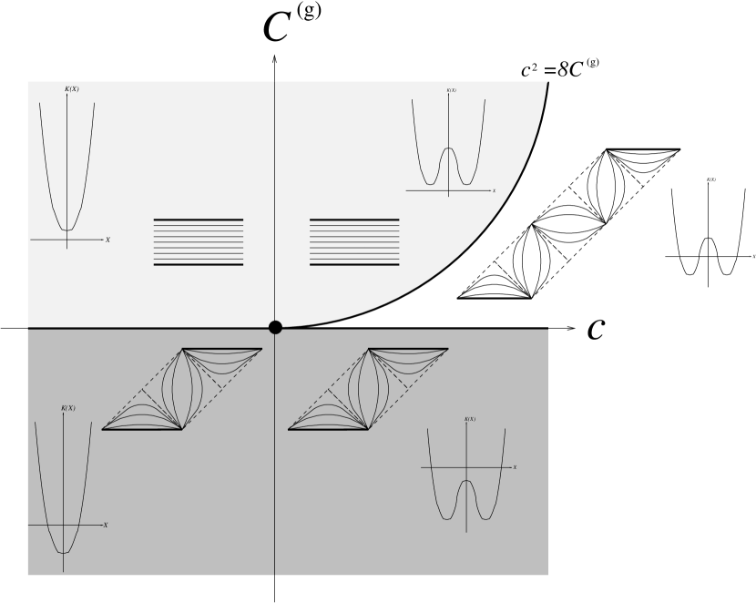
Figure 2: The phase space of building blocks for general CP diagrams. The white, dark gray and light gray region contains all CP diagrams with four, two and zero non-extremal Killing horizons, respectively. Bold lines in the phase diagram correspond to CP diagrams containing one or two extremal horizons (and possibly additional non-extremal ones). The point at the center corresponds to the special case $c=0=\mathcal{C}^{(g)}$ with an extremely extremal horizon (with fourth order zero in the Killing norm). The solution found in ref. [1] corresponds to the curved bold line separating the white from the light gray region. In the CP diagrams bold, dashed and ordinary lines correspond to curvature singularities, non-extremal Killing horizons and $X=\rm const.$ lines, respectively (only the non-extremal cases are depicted). The Killing norm as a function of $X$ also has been plotted in the five non-extremal regions (in the extremal limit zeros can be located at some of the extrema).

A straightforward generalization of the formulation (2) would be the consideration of arbitrary $\mathcal{V}(X^{+}X^{-},X,Y)$ instead of the special case (3). For all these models one Casimir function (corresponding to the total charge) becomes $Y=c$, while the other one is in general more complicated and related to the total energy. Possible applications of such models are twofold: if $Y$ appears at least quadratically in $\mathcal{V}$ it can be eliminated from the EOM obtained by varying with respect to $Y$ (not necessarily uniquely); in this case it represents the dual field strength (possibly with some coupling to the dilaton $X$). Such a situation is encountered e.g. for potentials of the type $\mathcal{V}=\tilde{\mathcal{V}}(X^{+}X^{-},X)+F(X)Y^{2}$ including the spherically reduced Reissner-Nordström black hole. If, however, $Y$ appears only linearly in the form $\mathcal{V}=\tilde{\mathcal{V}}(X^{+}X^{-},X)+F(X)Y$ as in the present case then the “dilaton” $X$ (or a function thereof) determines the dual field strength. This implies an interesting “gauge curvature to geometric curvature” coupling in the action which is explicit in the second order formulation (1).

Further generalizations are conceivable, e.g. the coupling to matter fields thus making the theory nontopological. In that case the virtual black hole phenomenon should be present [14] and interesting results can be derived within the path integral formalism [15].

Indeed, powerful methods to study these models classically, semi-classically and at the quantum level already do exist [2].

References

- [1] G. Guralnik, A. Iorio, R. Jackiw, and S. Y. Pi, “Dimensionally reduced gravitational Chern-Simons term and its kink,” hep-th/0305117.
- [2] D. Grumiller, W. Kummer, and D. V. Vassilevich, “Dilaton gravity in two dimensions,” Phys. Rept. 369 (2002) 327–429, hep-th/0204253.
- [3] N. Ikeda and K. I. Izawa, “General form of dilaton gravity and nonlinear gauge theory,” Prog. Theor. Phys. 90 (1993) 237–246, hep-th/9304012; N. Ikeda, “Two-dimensional gravity and nonlinear gauge theory,” Ann. Phys. 235 (1994) 435–464, arXiv:hep-th/9312059; P. Schaller and T. Strobl, “Poisson structure induced (topological) field theories,” Mod. Phys. Lett. A9 (1994) 3129–3136, hep-th/9405110; “Poisson sigma models: A generalization of 2-d gravity Yang- Mills systems,” in Finite dimensional integrable systems, pp. 181–190. 1994. hep-th/9411163. Dubna.
- [4] W. Kummer and P. Widerin, “Conserved quasilocal quantities and general covariant theories in two-dimensions,” Phys. Rev. D52 (1995) 6965–6975, arXiv:gr-qc/9502031.
- [5] A. S. Cattaneo and G. Felder, “A path integral approach to the Kontsevich quantization formula,” Commun. Math. Phys. 212 (2000) 591–611, math.qa/9902090.
- [6] B. M. Barbashov, V. V. Nesterenko, and A. M. Chervyakov, “The solitons in some geometrical field theories,” Theor. Math. Phys. 40 (1979) 15–27 and 572–581; J. Phys. A13 (1979) 301–312; E. D’Hoker and R. Jackiw, “Liouville field theory,” Phys. Rev. D26 (1982) 3517; C. Teitelboim, “Gravitation and Hamiltonian structure in two space-time dimensions,” Phys. Lett. B126 (1983) 41; E. D’Hoker, D. Freedman, and R. Jackiw, “SO(2,1) invariant quantization of the Liouville theory,” Phys. Rev. D28 (1983) 2583; E. D’Hoker and R. Jackiw, “Space translation breaking and compactification in the Liouville theory,” Phys. Rev. Lett. 50 (1983) 1719–1722; R. Jackiw, “Another view on massless matter - gravity fields in two- dimensions,” hep-th/9501016.
- [7] T. Klösch and T. Strobl, “Classical and quantum gravity in (1+1)-dimensions. Part I: A unifying approach,” Class. Quant. Grav. 13 (1996) 965–984, arXiv:gr-qc/9508020.
- [8] M. Walker, “Block diagrams and the extension of timelike two-surfaces,” J. Math. Phys. 11 (1970) 2280.
- [9] T. Klösch and T. Strobl, “Classical and quantum gravity in 1+1 dimensions. Part II: The universal coverings,” Class. Quant. Grav. 13 (1996) 2395–2422, arXiv:gr-qc/9511081.
- [10] T. Klösch and T. Strobl, “Classical and quantum gravity in 1+1 dimensions. Part III: Solutions of arbitrary topology and kinks in 1+1 gravity,” Class. Quant. Grav. 14 (1997) 1689–1723, hep-th/9607226.
- [11] T. Klösch and T. Strobl, “A global view of kinks in 1+1 gravity,” Phys. Rev. D57 (1998) 1034–1044, arXiv:gr-qc/9707053.
- [12] M. O. Katanaev, W. Kummer, and H. Liebl, “On the completeness of the black hole singularity in 2d dilaton theories,” Nucl. Phys. B486 (1997) 353–370, gr-qc/9602040.
- [13] M. Bojowald and T. Strobl, “Classical solutions for Poisson sigma models on a Riemann surface,” hep-th/0304252.
- [14] D. Grumiller, W. Kummer, and D. V. Vassilevich, “The virtual black hole in 2d quantum gravity,” Nucl. Phys. B580 (2000) 438–456, gr-qc/0001038; P. Fischer, D. Grumiller, W. Kummer, and D. V. Vassilevich, “S-matrix for s-wave gravitational scattering,” Phys. Lett. B521 (2001) 357–363, gr-qc/0105034; Erratum ibid. B532 (2002) 373; D. Grumiller, “Virtual black hole phenomenology from 2d dilaton theories,” Class. Quant. Grav. 19 (2002) 997–1009, gr-qc/0111097; D. Grumiller, W. Kummer, and D. V. Vassilevich, “Virtual black holes in generalized dilaton theories and their special role in string gravity,” hep-th/0208052, to be published in EPJC.
- [15] W. Kummer, H. Liebl, and D. V. Vassilevich, “Exact path integral quantization of generic 2-d dilaton gravity,” Nucl. Phys. B493 (1997) 491–502, gr-qc/9612012; “Integrating geometry in general 2d dilaton gravity with matter,” Nucl. Phys. B544 (1999) 403–431, hep-th/9809168; D. Grumiller, Quantum dilaton gravity in two dimensions with matter. PhD thesis, Technische Universität Wien, 2001. gr-qc/0105078; D. Grumiller, W. Kummer, and D. V. Vassilevich, “Positive specific heat of the quantum corrected dilaton black hole,” hep-th/0305036; D. Grumiller, “Three functions in dilaton gravity: The good, the bad and the muggy,” hep-th/0305073.